INTRODUCTION
Bottlenose dolphins (Tursiops truncatus) are large-bodied predators that can be locally abundant in coastal and estuarine habitats, including those of South Florida (Barros & Wells, Reference Barros and Wells1998; Mazzoil et al., Reference Mazzoil, Reif, Youngbluth, Murdoch, Bechdel, Howells, McCulloch, Hansen and Bossart2008; Urian et al., Reference Urian, Hoffman, Wells and Read2009). They have high metabolic rates, potentially imposing strong top-down effects on community structure through direct predation (Bowen, Reference Bowen1997; Young & Phillips, Reference Young and Phillips2002; Williams et al., Reference Williams, Estes, Doak and Springer2004). Therefore, understanding spatiotemporal variation in the abundance of dolphins is important for elucidating their potential ecological importance. In addition, understanding the drivers of habitat use and group size dynamics is critical to predicting how ecosystem changes may affect bottlenose dolphins and alter their ecological roles and importance.
Bottlenose dolphins are upper trophic level predators in oligotrophic mangrove estuaries of the Florida Coastal Everglades (FCE), which is comprised of multiple habitats including creeks, rivers, shallow inland bays that feature numerous mangrove islands, and coastal oceans of the Gulf of Mexico and Florida Bay. Over the past century, human alterations upstream have reduced freshwater flow in volume and duration, thus changing patterns of dissolved oxygen, salinity, primary production, and consequently the distribution of many species of consumers in the coastal Everglades (e.g. Turner et al., Reference Turner, Trexler, Jordan, Slack, Geddes, Chick and Loftus1999; Chick et al., Reference Chick, Ruetz and Texler2004; Rehage & Trexler, Reference Rehage and Trexler2006). Indeed, diminished freshwater flow has reduced fish populations, and in turn, limited populations of some predators (e.g. wading birds) though decreased food availability (Lorenz & Serafy, Reference Lorenz and Serafy2006; Trexler & Goss, Reference Trexler and Goss2009). How dolphins use the various habitats of the coastal Everglades and respond to seasonal variation in environmental conditions – including freshwater flow – is poorly known with the exception of several studies conducted in Florida Bay (Torres et al., Reference Torres, Read and Halpin2008; Torres & Read, Reference Torres and Read2009). Such an understanding is important, however, because the habitats of the FCE are predicted to be heavily impacted by sea level rise and the Comprehensive Everglades Restoration Plan (CERP), which is expected to increase freshwater inputs (Perry, Reference Perry2004; Davis et al., Reference Davis, Childers, Lorenz, Wanless and Hopkins2005; Gaiser, Reference Gaiser2009).
Previous work on large predators (bull sharks, Carcharhinus leucas; American alligators, Alligator mississipiensis) in the FCE suggest that they may play an important role in upstream transport of marine-derived nutrients into the oligohaline ecotone, but their movements and trophic interactions are influenced by both abiotic and biotic factors (e.g. Matich et al., Reference Matich, Heithaus and Layman2011; Rosenblatt & Heithaus, Reference Rosenblatt and Heithaus2011; Matich & Heithaus, Reference Matich and Heithaus2012, Reference Matich and Heithaus2014). However, sharks and alligators are poikilothermic and have low metabolic rates (Coulson et al., Reference Coulson, Herbert and Coulson1989; Schmid & Murru, Reference Schmid and Murru1994), particularly when compared with mammalian metabolism. Consequently, the overall ecological impacts of these species through consumptive effects may not be as sizeable as those of abundant mammalian predators like bottlenose dolphins (e.g. Bowen, Reference Bowen1997).
Habitat use and abundance of dolphins can be driven by numerous factors, including tidal variation (Gregory & Rowden, Reference Gregory and Rowden2001), the interaction of submarine characteristics with foraging tactics and seasonally abundant prey (Hastie et al., Reference Hastie, Wilson, Wilson, Parsons and Thompson2004), prey availability (Shane et al., Reference Shane, Wells and Wursig1986; Heithaus & Dill, Reference Heithaus and Dill2002), predation risk (Heithaus & Dill, Reference Heithaus and Dill2002, Reference Heithaus and Dill2006) and other environmental factors (Wilson et al., Reference Wilson, Thompson and Hammond1997; Barco et al., Reference Barco, Swingle, McLellan, Harris and Pabst1999; Miller & Baltz, Reference Miller and Baltz2010). The extent to which some of these relationships are causal, particularly for physical and abiotic drivers, remains unclear. For example, physical characteristics may indirectly affect dolphins through their impacts on the abundance and distribution of dolphin predators and prey (e.g. Toth et al., Reference Toth, Hohn, Able and Gorgone2011).
The objective of this study was to investigate seasonal and spatial variation in the abundance, group size and behaviour of bottlenose dolphins in the FCE to gain insights into their potential ecological roles and provide management-relevant information on dolphins in this unique habitat. Because predation risk could potentially affect seasonal and spatial variation in the abundance and habitat use of dolphins (Heithaus & Dill, Reference Heithaus and Dill2002, Reference Heithaus and Dill2006, see Kiszka et al., Reference Kiszka, Heithaus and Wirsing2015 for a review), we also investigated the prevalence of shark-inflicted injuries to bottlenose dolphins throughout the study area.
MATERIALS AND METHODS
Study site
The FCE extends from small creeks where freshwater marshes transition to mangrove forests through mangrove-lined channels and inland bays to the coastal oceans of the Gulf of Mexico and Florida Bay. The system is generally oligotrophic and phosphorus-limited with productivity decreasing from the mouths of rivers to upstream marshes (Childers et al., Reference Childers, Boyer, Davis, Madden, Rudnick and Sklar2006). During the dry season (January–June), salinities measuring >20 ppt may occur up to 17 km from the mouth of the estuary (Rosenblatt & Heithaus, Reference Rosenblatt and Heithaus2011) while salinities where the channels meet the coastal oceans can fall to <15 ppt in the wet season (July–December; Childers et al., Reference Childers, Boyer, Davis, Madden, Rudnick and Sklar2006). Fish from freshwater marshes enter creeks and channels during marsh dry down creating a pulse of prey for estuarine predators (Rehage & Loftus, Reference Rehage and Loftus2007).
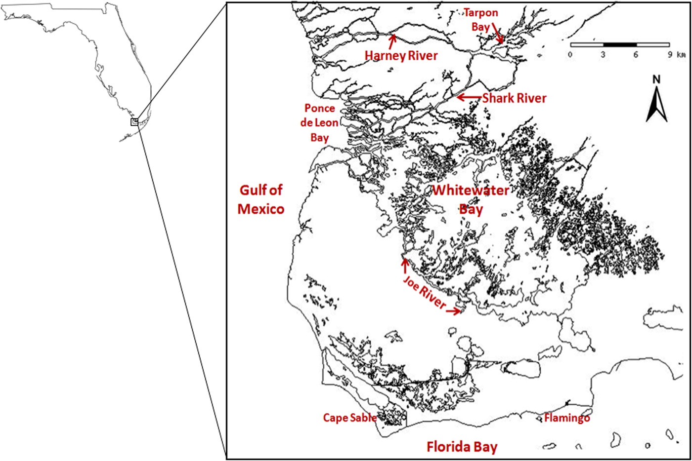
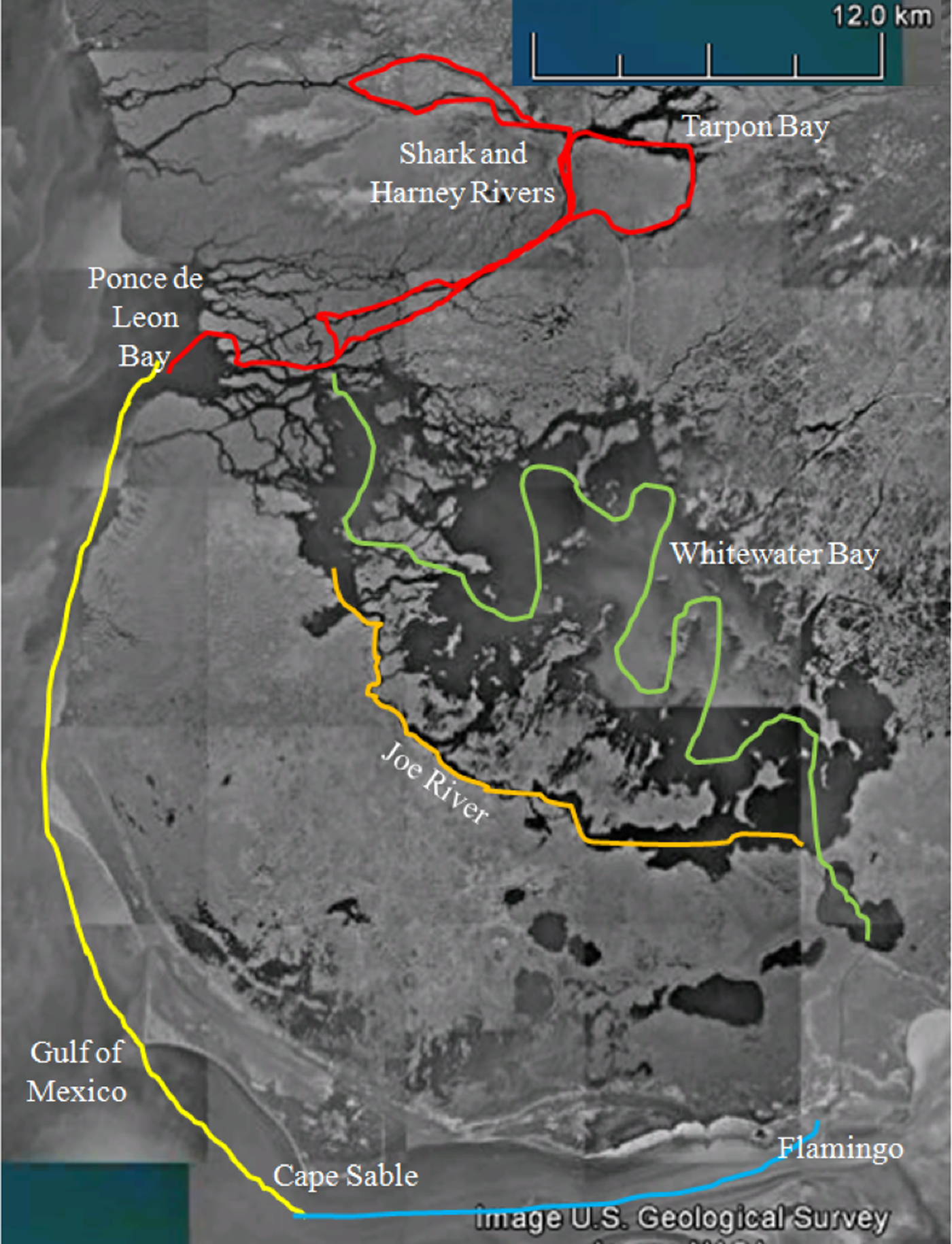
Fieldwork was conducted from July 2010–June 2012 in five major areas of the Everglades National Park: (1) Whitewater Bay, (2) Joe River, (3) Shark River Slough from Tarpon Bay to the mouths of the Harney and Shark Rivers, (4) coastal waters of Ponce de Leon Bay and a strip up to 4 km offshore and extending south to Cape Sable, and (5) north-western Florida Bay from Flamingo to Cape Sable (Figure 1).
The study was conducted in the coastal and inland waters of south-west Florida's coastal Everglades. Transects were conducted in the Shark and Harney Rivers, Joe River, Whitewater Bay, the Gulf of Mexico and Florida Bay.

Whitewater Bay is a large (~150 km2) and shallow enclosed bay with relatively uniform depth (0.75–1.75 m) and characterized by small tidal variation (rarely exceeding 0.4 m). Salinities range from 33 ppt in the dry season to as low as 5 ppt in the wet season (unpublished data). Numerous small islands covered by red mangroves (Rhizophora mangle) are scattered throughout the bay. Joe River is a medium depth channel (1.5–2 m depth; average width 150 m), with numerous connections to Whitewater Bay.
The Shark and Harney Rivers are comprised of deeper water channels (2.5–4.5 m deep, with an average width of 100 m) lined with mangroves and a salinity gradient ranging from up to 35 ppt at the river mouth during the dry season to values <4 ppt in Tarpon Bay during the wet season. Tarpon Bay is a narrow (100–500 m), shallow (1–2 m), mangrove-lined bay bordering the sawgrass ecotone. Ponce de Leon Bay and the portion of the coastal Gulf of Mexico used in this study are 2.5–4.5 m depth with a sand/silt benthos and salinities of 25–35 ppt (R. Sarabia, unpublished data). Florida Bay is a shallow basin, connected to the Gulf of Mexico at its western margin and to the Straits of Florida to the south through multiple channels between the islands of the Florida Keys. Mean salinity during the dry season can exceed 40 ppt in the areas surveyed (Boyer et al., Reference Boyer, Fourqurean and Jones1997). Water clarity, depth and benthic habitats vary regionally; the area covered by this study is characterized by a patchwork benthos of mud, sand, and patchy seagrass (the most common species are Thalassia testudinum, followed by Halodule wrightii and Syringodium filiforme; Zieman et al., Reference Zieman, Fourqurean and Iverson1989), very turbid water and depths ranging from 0.5 to 3 m (Torres & Read, Reference Torres and Read2009).
Study methods
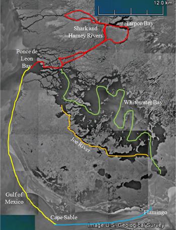
We established belt transects in five regions (three estuarine, two in the coastal ocean): Whitewater Bay (55 km), the Shark and Harney Rivers and Ponce de Leon Bay (51 km), Joe River (21 km), the coastal waters of the Gulf of Mexico (33 km) and Florida Bay (20 km, Figure 2). Transect locations were set based on the survey methods for an estuarine/riverine environment described in Read et al. (Reference Read, Urian, Wilson and Waples2003). Transects were surveyed from a 6.4 m vessel with three to four trained observers, and run in random order and direction. Transects were driven at 15 km h−1 and only in Beaufort wind conditions 3 or less.
Location of sampling transects in the Florida Coastal Everglades. Image from Google Earth 6.1.
When a dolphin group was encountered standard group data were recorded, including geographic position and group characteristics (best group size estimate, composition, predominant behavioural activity). A group was defined as all animals in close proximity to one another (<100 m) engaged in similar behaviours (Shane, Reference Shane, Leatherwood and Reeves1990). Habitat type at the position of initial encounter and distance to nearest land were also recorded. Habitat type was defined as bay (estuarine waters wider than 0.5 km), channel (estuarine waters narrower than 0.5 km) or nearshore (open waters not contained within the estuary). The predominant behavioural activity (or activity) was determined at first sighting and was defined as the behavioural state in which most animals of the group were involved. Activity was categorized according to a modification of the Sarasota Bay Research Program guidelines (e.g. McHugh et al., Reference McHugh, Allen, Barleycorn and Wells2011). Travelling dolphins were those seen surfacing with persistent directional movement and surfacing at regular intervals. Resting dolphins were observed at or near the surface but not engaged in any obvious surface and directional behaviour, exhibited slow movements, and usually occurred in tight formation. Socializing dolphins were those observed chasing or making bodily contact with one another, including a suite of possible behaviours linked with play and/or mating. Foraging dolphins were those observed making any effort to capture prey. Behaviours included, but were not limited to, tail-out grubbing in the mud, herding prey, chasing prey, and rapid surfacing at varying intervals with no consistent heading. If the dolphins were first observed reacting to the presence of the researchers (e.g. approaching the boat to bow ride) or if their behaviour was not observed long enough to be classified, their behaviour was classified as ‘Unknown’.
We took photographs of the dorsal fins of every individual in a group using a Canon EOS 10D SLR. These photos were used to create a catalogue of dorsal fins to identify individuals based on variation in dorsal fin size and shape, along with the nicks and scars acquired through the animal's lifetime (Wursig & Wursig, Reference Wursig and Wursig1977). The sex of animals was determined opportunistically, either by observing the presence of a dependent calf in the echelon position with a particular animal across multiple surveys, or by directly observing the external genitalia (when animals were bow riding). Calves were identified by size and behaviour and sorted into three categories: juveniles, calves and neonates. Juveniles were defined as animals smaller than adult size but greater than half an adult body length. A calf was defined as an animal smaller than half an adult body length, and was typically found closely associated with its mother, particularly while surfacing. Neonates were identified by the presence of visible foetal folds and stereotypical awkward surfacing during breathing (Mann & Smuts, Reference Mann and Smuts1999).
Photographs were also used to examine individuals for evidence of scars from shark bites. Scars were considered to have been inflicted by sharks if they were characteristically crescent-shaped or had deep and widely spaced tooth marks (Heithaus, Reference Heithaus2001). We determined the proportion of individuals with wounds by comparing the number of known individuals with wounds to the total number of individuals identified. This method underestimates the actual proportion of individuals with wounds since only a small portion of the body is surveyed for evidence of shark bites (Heithaus, Reference Heithaus2001).
Data analysis
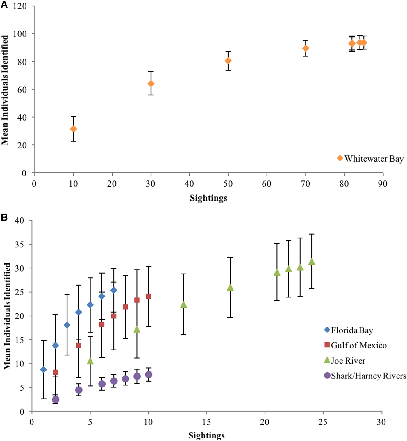
Statistical tests were carried out using JMP Pro 10™ software. To test for adequate sampling, a rarefaction analysis was performed. Cumulative individual curves were generated by resampling group compositions for 1000 random iterations to calculate a mean and variability estimate of the cumulative number of individuals for each group. This mean cumulative number of individuals was then plotted against the randomly pooled number of groups; a linear regression was then performed on the last four points to determine if the slope of the line was significantly different from zero (e.g. Bizzarro et al., Reference Bizzarro, Robinson, Rinewalt and Ebert2007).
To determine spatial and temporal variation in dolphin abundance, we calculated both the densities of groups (groups km−2) and individuals (individuals km−2), as well as the densities of foraging individuals (foraging individuals km−2). Area sampled per transect was calculated by multiplying transect length by average channel width (derived from measurements every 100 m along transects). If channel widths were more than 0.8 km, we truncated transects to a belt extending 400 m to each side of the boat. Groups beyond 400 m were eliminated from analyses. The total surface areas surveyed across the study site during a single transect pass were 33 km2 in Whitewater Bay, 5 km2 in Shark and Harney Rivers, 5 km2 in Joe River, 26.4 km2 along the coastal waters of the Gulf of Mexico, and 16 km2 in Florida Bay.
To assess differences in densities by region, habitat type and season, we performed a series of generalized linear models (GLMs) with a quasi-poisson distribution and a log(area) offset followed Tukey's tests, which correct for multiple comparisons, to compare means. A series of logistic regressions were run to investigate how the probability of encountering dolphins was affected by habitat type (mangrove, channel or open), season, and any interactions. For each square kilometre within a transect, the season, region, presence or absence of land within 400 m of the transect line, distance to land, and habitat type were recorded. We also recorded the presence or absence of (1) dolphins, (2) dolphins with calves and (3) foraging dolphins, as well as the total numbers of adults, calves and foraging individuals. We used logistic regression to determine if dolphins preferentially used areas near mangrove islands in Whitewater Bay, by comparing the presence or absence of dolphins during each transect pass within 100 m of mangrove islands relative to that more than 100 m from islands.
The turbidity of water usually limited our ability to simultaneously view all individuals in a group and some individuals were indistinguishable because of similar fin shapes and a lack of natural markings. Therefore, we calculated group size using the best field estimate supplemented by photoidentification. These data were non-normal, and transformations were not successful. Therefore, we used a series of Kruskal–Wallis tests to investigate the effects of season (Wet or Dry), group composition (the presence or absence of calves), behaviour (at first sighting), and region on group size. For tests showing significant effects, Mann–Whitney tests were used to determine statistically significant paired contrasts where necessary.
RESULTS
Sampling and photo-identification data
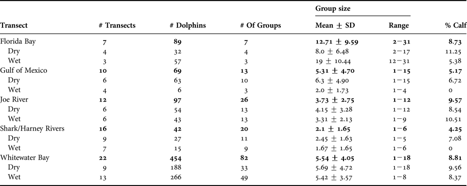
From August 2010–June 2012, we completed a total of 67 transects (34 in the dry season, 33 in the wet season). These transects involved over 268 h of observation and covered c. 2650 linear km and 1232 km2 (Table 1). We encountered 148 groups of bottlenose dolphins, 34 of which were foraging, 14 were socializing, and 63 were travelling. We were not able to determine the behaviour of 27 groups. Obviously resting groups of dolphins were not observed. Multiple foraging behaviours were observed; the most common behaviour was a tail-out mud grubbing behaviour that was observed 15 times by groups of 1–18 individuals, while using mangrove roots to herd fish was observed on seven occasions by groups of 1–5 individuals. Intentional stranding on mud banks was opportunistically observed near the mouth of the Harney River on two occasions by groups of two and three individuals. We were unable to identify prey during our observations.
Seasonal and regional survey effort and dolphin sightings.

Values in bold font represent pooling of dry and wet season data.
Over 12,000 photographs resulted in identifying 174 unique individuals. A total of 31 animals were identified in Florida Bay, 30 in the Gulf of Mexico, 9 in the Shark and Harney Rivers, and 92 in Whitewater Bay. All 14 individuals identified in Joe River were also observed in Whitewater Bay. Three animals were observed using both western Whitewater Bay and the Shark River, four were observed using both the coastal ocean and either western Whitewater Bay or Shark River, and two animals were observed in both Florida Bay and the Gulf of Mexico. No animals from the estuary were observed in Florida Bay or vice versa. Definitive shark bite scars were observed on only two identifiable individuals, both seen in Whitewater Bay, with possible bites recorded for seven others resulting in a minimum estimate of 1–5% of the population having been bitten by sharks along their dorsal surfaces.
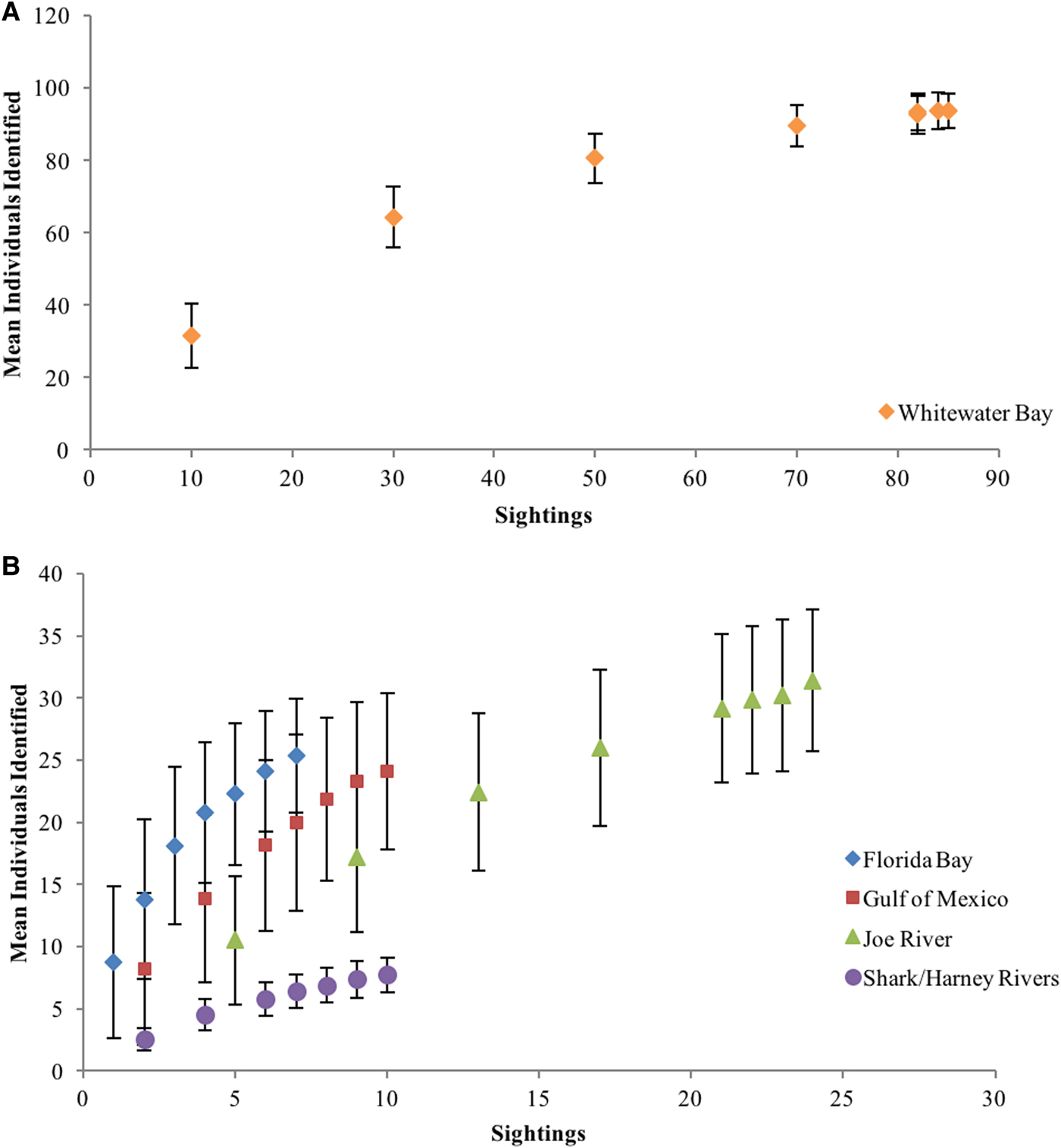
Identification rates of new individuals in Whitewater Bay reached an asymptote at 93 individuals with a non-significant slope (P = 0.09; Figure 3A). In contrast, the slopes of the identification rates of new individuals in Florida Bay (P = 0.003), the Gulf of Mexico (P = 0.012), Joe River (P = 0.02) and the Shark and Harney Rivers (P = 0.002) were all significantly different from zero, indicating that new individuals were still being discovered (Figure 3B).
Cumulative individual curves generated by resampling group compositions for 1000 randomly selected groups within Whitewater Bay (A) and the four other regions of the study area (B). Points show means, error bars show SD.
Spatiotemporal variation in densities
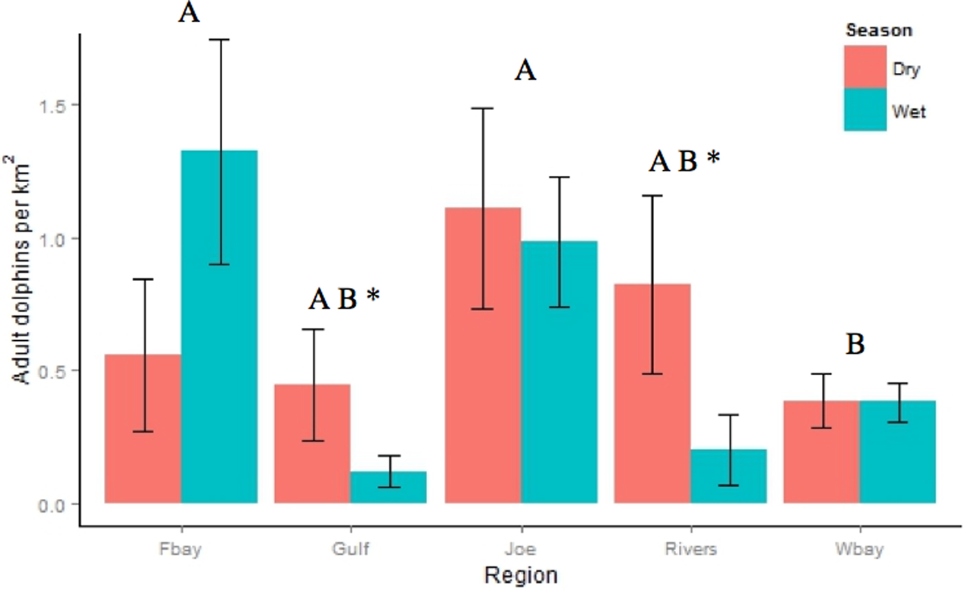
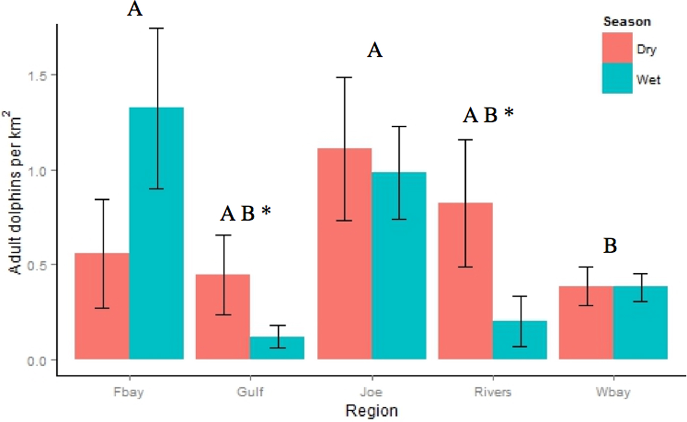
The density of individuals (Figure 4) varied significantly among regions. Densities were significantly higher in Joe River (mean = 1.06 dolphins km−2 ± 0.93 SD) (Z = −4.46, P < 0.001) and Florida Bay (mean = 0.88 dolphins km−2 ± 0.72) (Z = −3.11, P = 0.015) than in Whitewater Bay (mean = 0.38 dolphins km−2 ± 0.41). Densities only varied significantly across seasons in the Gulf of Mexico (T = −2.14, P = 0.035), with higher dolphin densities during the dry season (mean = 0.45 dolphins km−2 ± 0.52) than the wet season (mean = 0.12 dolphins km−2 ± 0.11). Although we measured higher dolphin densities during the dry season (mean = 0.82 dolphins km−2 ± 1.01) than the wet season (mean = 0.20 dolphins km−2 ± 0.35), this difference was not statistically significant (T = −1.86, P = 0.066).
Spatiotemporal variation in the density of dolphins in the Florida Coastal Everglades (FBay: Florida Bay; Gulf: Gulf of Mexico; Joe: Joe River; Rivers: Shark and Harney Rivers; Wbay: Whitewater Bay) expressed as the number of animals encountered per km2. Bars show mean values; bars with the same letter are not significantly different from one another. * indicates a significant difference between wet and dry seasons within a region.
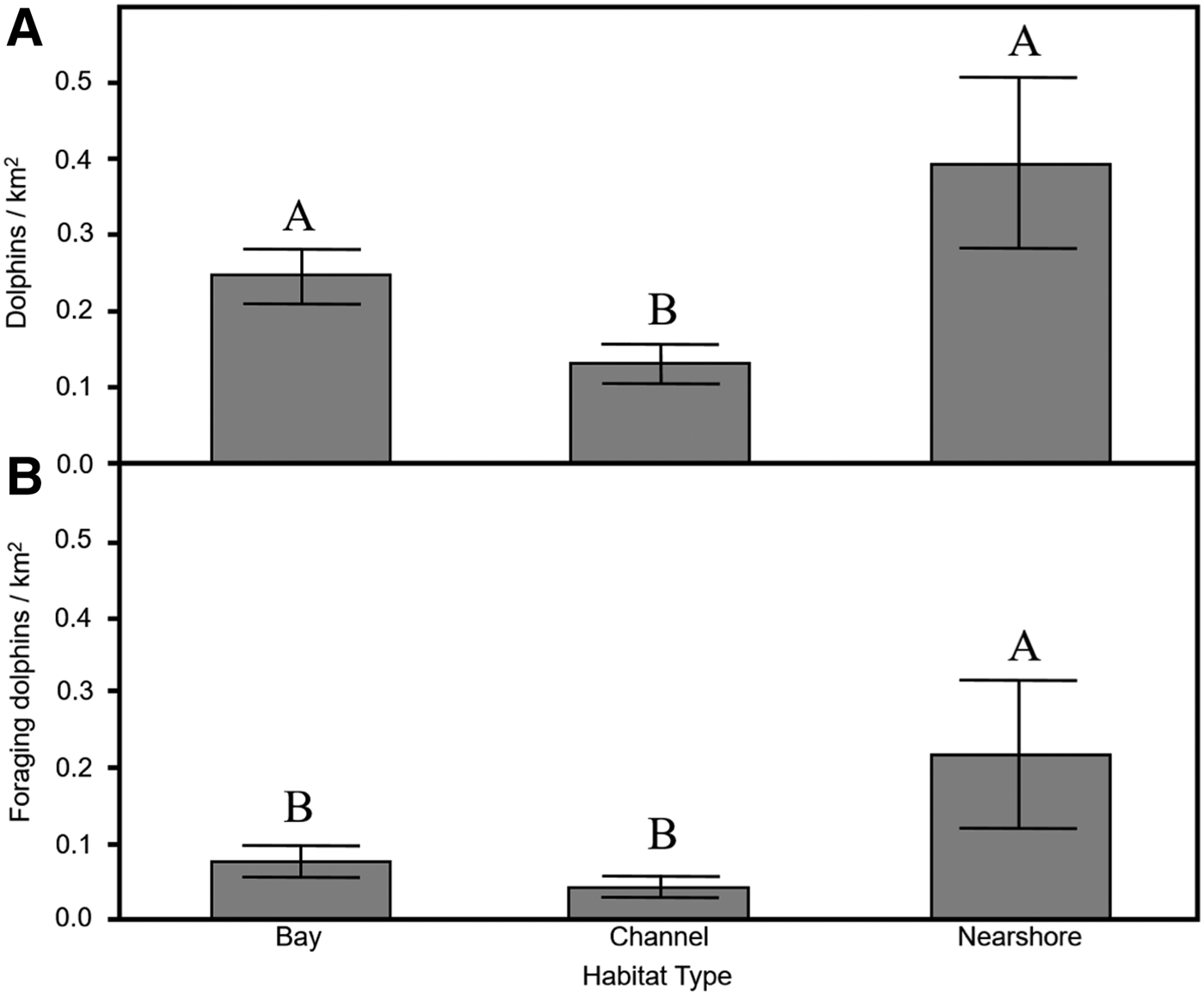
The probability of encountering groups was higher within 100 m of islands than in waters more than 100 m from islands (Z = 4.58, P = 0.03). The probability of encountering groups also varied with habitat, with fewer groups encountered in channels than in either the nearshore area or open estuarine bay habitats (F = 5.69, P = 0.003) (Figure 5A).
Density of all dolphins (A) and foraging dolphins (B) by different habitat types in the Florida Coastal Everglades expressed as the number of animals encountered per km2. Bars show mean values; bars with the same letter are not significantly different from one another.

The likelihood of encountering a foraging group varied by region (F = 5.17, P = 0.004) with the highest encounter probabilities in Joe River and the lowest in Whitewater Bay and the Shark and Harney Rivers. The probability of encountering foraging groups varied with habitat (F = 4.60, P = 0.01). They were found in Florida Bay and the Gulf of Mexico more often than Whitewater Bay or rivers habitat (Figure 5B).
Group size
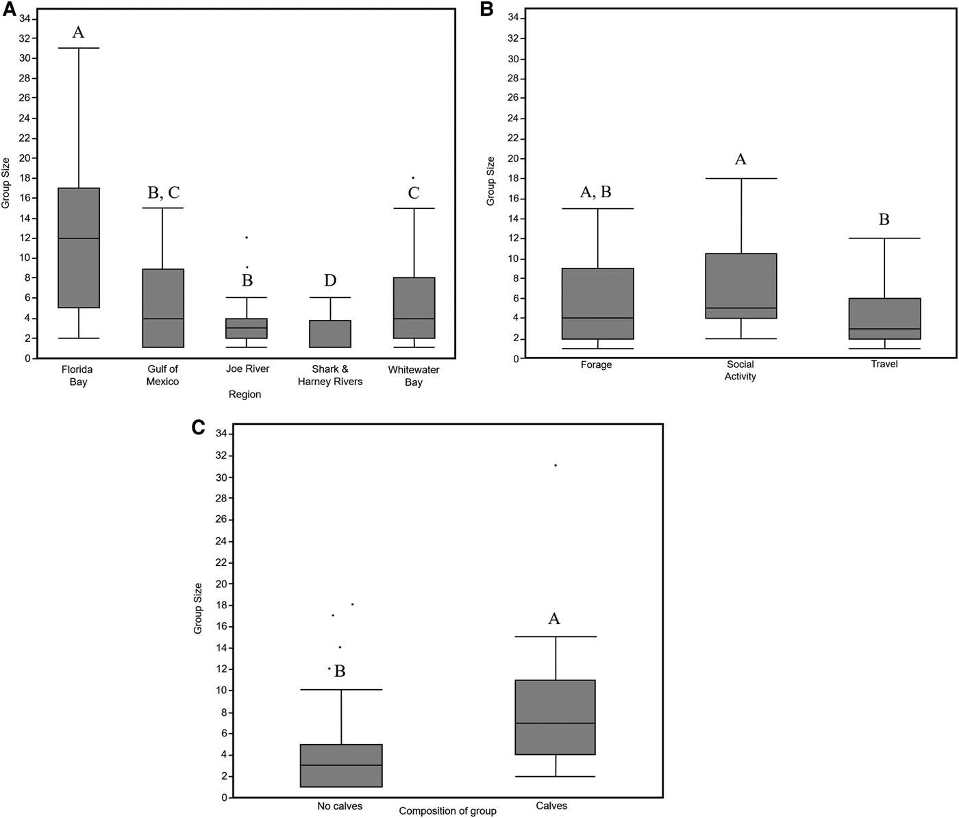
Group sizes varied across regions (Kruskal–Wallis, K = 25.88, P < 0.0001) and among habitats within Whitewater Bay (Kruskal–Wallis, K = 17.24, P = 0.0002). The smallest groups were found in Harney, Joe and Shark rivers and the largest were found in Florida Bay. Mean group sizes were intermediate in the Gulf of Mexico, Joe River and Whitewater Bay (Figure 6A). We did not detect seasonal variation in group sizes among or within regions (Kruskal–Wallis; K = 0.84, P = 0.89).
Variation in group sizes among regions (A), estuarine habitats (B), and presence or absence of calves (C). Boxplots show median, quartile, minimum and maximum.

Group size varied among behavioural states (Kruskal–Wallis statistic K = 12.72, P = 0.005). Travelling groups were significantly smaller than the socializing groups. Foraging group sizes were not significantly different from either socializing or travelling groups (Figure 6B). Groups with juveniles, calves or neonates were much larger than those without younger age classes within estuarine regions (Kruskal–Wallis test = 15.60, P = 0.004) (Figure 6C).
DISCUSSION
Bottlenose dolphins are common in coastal and estuarine habitats around the world (e.g. Wells & Scott, Reference Wells, Scott, Ridway and Harrison1999; Connor et al., Reference Connor, Wells, Mann, Read, Mann, Connor, Tyack and Whitehead2000), and the FCE provides an excellent study site thanks to the considerable diversity of habitat types (coastal oceanic waters, brackish rivers and bays) present. In addition, most studies of estuarine dolphins have occurred in areas with relatively high human densities (e.g. Barros & Wells, Reference Barros and Wells1998; Gregory & Rowden, Reference Gregory and Rowden2001; Hastie et al., Reference Hastie, Wilson, Wilson, Parsons and Thompson2004). Although water flow into the FCE is highly modified and managed by humans, the current study site is typified by low densities of boats and relatively few direct human impacts (Ault et al., Reference Ault, Smith, McClellan, Zurcher, McCrea, Vaughan and Bohnsack2008) that could potentially alter dolphin distribution and abundance (Bejder et al., Reference Bejder, Samuels, Whitehead, Gales, Mann, Connor, Heithaus, Watson-Capps, Flaherty and Krützen2006). We found that in spite of considerable seasonal variation in conditions – including temperature, salinity and influxes of prey from marsh habitats – bottlenose dolphins in this temporally dynamic environment exhibit relatively stable densities and group sizes within regions, but show considerable variation in their use of regions in the estuary and coastal ocean.
There appears to be a year-round residential population, at least in Whitewater Bay and Joe River. Indeed, 45 out of 50 individuals encountered on more than four sampling days were observed at least once in each season. The presence of either a seasonal resident or a transient portion of the population is possible within the FCE, however, since 125 animals were observed three times or fewer, with 62 animals sighted only once. Of the individuals sighted only once, 36 were from the Gulf of Mexico or Florida Bay. Further work is needed to determine if these rarely sighted individuals are transient or are part of a resident population but are not frequently encountered because the survey transects only included a small portion of their home ranges. In general, the rivers appear to be used infrequently by dolphins and the individuals that use these habitats may not do so consistently. Future social network, genetic or isotopic studies may help elucidate population and community structure of bottlenose dolphins in the coastal Everglades region (e.g. Urian et al., Reference Urian, Hoffman, Wells and Read2009; Kiszka et al., Reference Kiszka, Simon-Bouhet, Gastebois, Pusineri and Ridoux2012; Olin et al., Reference Olin, Fair, Recks, Zolman, Adams and Fisk2012).
With overall densities of 0.38–1.06 dolphins km−2 within the estuarine Everglades, this area appears to have moderate to high densities compared with nearby coastal populations. For example, densities of 0.3 dolphins km−2 were observed in coastal Louisiana (Mullin et al., Reference Mullin, Lohoefener, Hoggard, Roden and Rogers1990), 0.77 dolphins km−2 off the west Florida continental shelf (Griffin & Griffin, Reference Griffin and Griffin2004), 1.3 dolphins km−2 in Sarasota Bay (Irvine et al., Reference Irvine, Scott, Wells and Kaufmann1981) and 0.23–0.68 dolphins km−2 in various estuaries along the south-eastern coast of the United States (Leatherwood, Reference Leatherwood1979).
Dolphin densities varied somewhat among regions. Densities were higher in Florida Bay and Joe River than in Whitewater Bay. Interestingly, density was least variable in Whitewater Bay, which, combined with Whitewater Bay's high rates of re-sighting suggests a residential population. The density of dolphins along the coast of the Gulf of Mexico and the rivers was higher in the dry season, which may reflect individuals shifting home ranges slightly or an influx of new individuals that move more broadly along the Florida coast. Such density increases could reflect individuals taking advantage of foraging opportunities. During the dry season there is a pulse of freshwater fish entering the rivers as marsh taxa seek refuge from drying marshes (Rehage & Loftus, Reference Rehage and Loftus2007). Alternatively, increases in salinity during the dry season may reduce the physiological costs of accessing prey in the coastal estuarine and riverine waters. Stable isotope (Matich et al., Reference Matich, Heithaus and Layman2011; Rosenblatt & Heithaus, Reference Rosenblatt and Heithaus2011) and fatty acid (Belicka et al., Reference Belicka, Matich, Jaffe and Heithaus2012) analysis could provide insights into the contribution of freshwater and estuarine taxa to the diets of dolphins using river habitats.
It was somewhat surprising that densities were considerably higher in Joe River than the adjacent Whitewater Bay since they should experience very similar water temperatures and salinities throughout the year. In addition, all of the individuals observed in Joe River were also observed in Whitewater Bay at some time. In other locations (e.g. Shark Bay, Australia; Heithaus & Dill, Reference Heithaus and Dill2002) spatial variation in predation risk can drive differences in habitat use. This seems unlikely in this case because the abundance of large sharks is low in Whitewater Bay and Joe River (Wiley & Simpfendorfer, Reference Wiley and Simpfendorfer2007) and proportions of individuals with shark-inflicted injuries are low (see below). Dolphins may use Joe River for foraging reasons. Dolphins may use the greater proportion of mangrove-lined shores to facilitate foraging. There is some evidence this might be occurring with dolphin groups in Whitewater Bay found more often near mangrove-lined islands than in more open waters. Similarly, in the Moray Firth, dolphins preferentially forage over steep seabed gradients that may either provide higher concentrations of prey or increased foraging efficiency (Hastie et al., Reference Hastie, Wilson, Wilson, Parsons and Thompson2004).
The proportion of individuals with scars or wounds from shark bites was quite low (1–5%) compared with some other locations. For example, boat-based observations of free-swimming animals documented scars of 74.2% of individuals in Shark Bay (Heithaus, Reference Heithaus2001) and 36.6% of individuals in Moreton Bay, Australia (Corkeron et al., Reference Corkeron, Morris and Bryden1987). In Sarasota Bay, the proportion of individuals with shark-inflicted wounds is lower. Even though animals were captured and the entire body was assessed, only 31% of individuals had evidence of having been bitten by sharks (Urian et al., Reference Urian, Wells, Scott, Irvine, Read and Hohn1998). It is likely that some of the differences in the proportion of individuals with scars or wounds between the FCE and these locations are driven by poorer observation conditions in the FCE (e.g. turbid waters, free-swimming animals). When viewed in light of low catch rates of large sharks within the FCE (e.g. Wiley & Simpfendorfer, Reference Wiley and Simpfendorfer2007; P. Matich unpublished data), however, scarring data suggest that predation risk for bottlenose dolphins is relatively low in the FCE.
Predation rates need not be high in order to elicit strong anti-predator behaviour, and the low incidence of shark-inflicted injuries could be the result of effective anti-predator behaviour (e.g. Lima & Dill, Reference Lima and Dill1990). Indeed, even though predation pressure is relatively low in Sarasota Bay, dolphins were still found to preferentially use shallower, more complex habitats during the times when bull sharks were most prevalent (Wells et al., Reference Wells, Irvine, Scott and Herman1980). In delphinids, group sizes generally increase with increasing predation risk (Gygax, Reference Gygax2002) and also tend to be lowest in species that do not experience predation risk (e.g. river dolphins; Gomez-Salazar et al., Reference Gomez-Salazar, Trujilo and Whitehead2012). Group sizes, however, are mediated by costs such as increased probabilities of predator and parasite encounter and resource competition (Bertram, Reference Bertram, Krebs and Davies1978). For coastal populations of bottlenose dolphins, group sizes are typically smaller where the habitat is complex and resources are predictable (e.g. Campbell et al., Reference Campbell, Bilgre and Defran2002) and larger in open water with unpredictable and spatially fluctuation resources (e.g. Defran & Weller, Reference Defran and Weller1999). For example, in Sarasota Bay, the largest groups are ‘nursery bands’ comprised of loosely associated females and their calves. These groups select different parts of the population's home range than male pairs or mixed-sex juvenile groups; nursery bands select protected shallow-waters much more often than subadults or males (Wells, Reference Wells, Roat, Ciccolella, Smith and Tomasko1993).
The Comprehensive Everglades Restoration Project (CERP) is poised to modify the volume and timing of fresh water released into the coastal estuaries of Everglades National Park. This will result in reduced salinities through portions of the current study system and will probably modify the dynamics of prey pulses moving from marsh to mangrove-lined channels that dolphins can access. Based on our data, it is possible that such changes in abiotic and biotic conditions could result in reduced densities of dolphins in some habitats. Long-term studies will allow more detailed investigations of the factors impacting dolphin densities and habitat use and provide insights into probable responses to changes induced by Everglades restoration. In addition, future research incorporating stable isotopic or fatty acid analysis would provide insights into the foraging ecology of dolphins and be an important first step in elucidating their ecological roles in the FCE.
ACKNOWLEDGEMENTS
We thank J. Lewis, A. Rosenblatt, D. Burkholder, K. Gastrich and P. Matich and all our volunteers for their invaluable help in data collection, and R. Nowicki for his help at all stages of this project. This is contribution #42 of the Marine Education and Research Center in the Institute for Water and Environment at Florida International University.
FINANCIAL SUPPORT
This project was part of the Florida Coastal Everglades Long Term Ecological Research Project with funding provided by the National Science Foundation (DBI0620409, DEB9910514, DRL0959026).