





Introduction
Marine species are exposed to natural and anthropogenic sounds (Hildebrand Reference Hildebrand2009), and anthropogenic sounds are reaching increasingly remote habitats, including the depths of the ocean (Dziak et al. Reference Dziak, Haxel, Matsumoto, Lau, Heimlich and Nieukirk2017). For marine mammals, a group highly sensitive to sound, responses to increased sound exposure include changing orientation (Cox Reference Cox2006), speed (Nowacek et al. Reference Nowacek, Johnson and Tyack2004), respiration (Frankel & Clark Reference Frankel and Clark2000) and group distribution (Frankel & Clark Reference Frankel and Clark2000), avoidance (Erbe et al. Reference Erbe, Dunlop, Dolman, Slabbekoorn, Dooling, Popper and Fay2018), aggressive behaviour (Southall et al. Reference Southall, Bowles, Ellison, Finneran, Gentry and Greene2007) and suppression of reproduction (Southall et al. Reference Southall, Bowles, Ellison, Finneran, Gentry and Greene2007). These effects can lead to interruptions in foraging (Pirotta et al. Reference Pirotta, Merchant, Thompson, Barton and Lusseau2015), increased vulnerability to predation (Simpson et al. Reference Simpson, Radford, Nedelec, Ferrari, Chivers, McCormick and Meekan2016) and decreased lifespans (Erbe et al. Reference Erbe, Dähne, Gordon, Herata, Houser and Koschinski2019), resulting in both individual-fitness and population-level effects (Harwood et al. Reference Harwood, King, Schick, Donovan and Booth2014).
In this study, we non-invasively investigated whether a common coastal marine top predator, the common bottlenose dolphin (Tursiops truncatus), altered its spatial location and movements under differing ambient sound conditions. Previous passive acoustic monitoring studies localized dolphin clicks (Aubauer et al. Reference Aubauer, Lammers and Au2000), whistles from a towed array (Quick & Janik Reference Quick and Janik2012) or in captivity (Freitag & Tyack Reference Freitag and Tyack1993), or they used direct observations of dolphins, but this study utilized a moored array to localize dolphins in the open ocean and assess their movements.
We hypothesized that dolphins would increase their speed of travel, travel in more direct routes and utilize a smaller area during higher sound conditions to maintain group cohesion (Erbe et al. Reference Erbe, Dunlop, Dolman, Slabbekoorn, Dooling, Popper and Fay2018). We also expected a greater response to increased mid-frequency sound levels compared to broadband levels due to bottlenose dolphins’ hearing sensitivity and communication within this range (4200–11 900 Hz; Jensen et al. Reference Jensen, Beedholm and Wahlberg2014).
Materials and methods
Study area
Our study area was located in the southern Mid-Atlantic Bight, USA, between 26 and 30 km east of Ocean City (MD, USA). This area contains the proposed wind energy area (WEA) offshore of Maryland and is adjacent to the Port of Wilmington (Delaware) traffic separation scheme. Water depths ranged from 25 to 28 m, and the recording units were deployed 3 m above the ocean floor using bottom-anchored moorings.
Data collection
Acoustic recordings were obtained using an array of marine autonomous recording units (MARUs; Cornell University, NY, USA) with a mean of 2.76 km between units deployed from July through August 2018. MARUs were equipped with an HTI-94-SSQ hydrophone (High Tech, Inc., MS, USA; sensitivity: –162 dB re 1 V/µPa, frequency response: 2 Hz–30 kHz) sampling at 16 kHz. High-pass (10 Hz) and low-pass (7080 Hz) filters were applied to the acoustic data. The four MARUs (Fig. 1) recorded continuously and were time-synchronized using known-source playbacks at the beginning and end of the deployment. No sightings, taggings or focal follows were used to validate acoustic detections due to the temporal and spatial logistics of the study site. Water temperature and salinity were relatively consistent throughout the deployment, so the same speed of sound was used in all calculations.
Ambient sound analysis
Ambient sound levels at A-2M were calculated using the RAVEN X toolbox (Dugan et al. Reference Dugan, Klinck, Roch and Helble2016) in MATLAB (Mathworks, Inc., MA, USA) as representative sound levels of the region. Sound levels (dB re 1 µPa root mean square; hereafter: dBrms) were computed for each 1-s time bin and 1-Hz frequency band with a Hann window with zero overlap and fast Fourier transformation (FFT). The metric of equivalent continuous sound pressure level or Leq (dBrms) was used to represent the average unweighted sound level of a continuous time-varying signal of pressure.
Hourly sound level averages were calculated for the broadband (10–7080 Hz) and mid-frequency (2820–7080 Hz) sound levels and sound-level categories (SLs) were split into the lower 25%, middle 50% and upper 25% of sound levels during the recording period. While hourly sound levels do not capture the instantaneous sound levels and do not remove the contribution of whistles to ambient sound levels, this metric related the sound level to dolphin movement characteristics within that time.
Dolphin whistle detection and localization
Common bottlenose dolphins are the primary marine mammal species present during the summer months in this region (Barco et al. Reference Barco, Swingle, McLellan, Harris and Pabst1999). Acoustic recordings were processed using the PAMGUARD Whistle and Moan Detector (Gillespie et al., Reference Gillespie, Palmer, Macaulay, Sparling and Hastie2020) to identify when dolphin whistles were present as an indicator of dolphin presence. Acoustic data were manually reviewed, and localization was conducted using Raven 2.0 (256-pt FFT, Hann window, 75% overlap, frequency resolution of 62.5 Hz, time resolution of 4 ms; K. Lisa Yang Center for Conservation Bioacoustics 2019) Correlation Sum Estimation (CSE) localization algorithm (Appendix S1; Hawthorne & Salisbury Reference Hawthorne and Salisbury2016).
To determine the precision of the CSE algorithm, 100 randomly selected whistles in each SL (300 whistles total) were localized five times, yielding five location estimates for each. We determined the mean distance of each location from the centre of the localization array and the mean distance between all five location estimates, and we used an analysis of variance (ANOVA) to determine whether the distance between locations varied depending on the SLs in which they were detected.
Dolphin spatial distribution
Kernel density estimates of the 100 randomly selected dolphin localizations (using the mean location of all five localizations) in each broadband and mid-frequency SL were calculated using the Home Range Tool (Rodgers et al. Reference Rodgers, Kie, August, Rodgers and Kie2011) in ArcGIS 10.4 (esri.com). A Wilcoxon rank-sum test was used to determine whether the areas of the 25th, 50th, 75th and 90th kernel density percentiles significantly differed in relation to the ambient SLs. ANOVAs and Tukey’s post-hoc analyses (Tukey-HSD) were utilized to investigate whether and how the spatial distribution (latitude and longitude) of the dolphins’ locations varied under different SLs.
Dolphin movement patterns
The detection range of the localization array was estimated to be 15 km from the centre of the array based on the source level of dolphin whistles (138 dBrms; Frankel et al. Reference Frankel, Zeddies, Simard and Mann2014). Whistles were numerous in the recordings (hundreds of thousands). For this analysis, we resampled across the recording period to obtain 14 random hours with whistles in each broadband SL (42 h total). While there is some overlap, this subsample of whistles was different from the 100 randomly selected localizations selected for the spatial distribution analyses. All whistles within these hours that had fewer than 10 min between whistles were selected for localization to assess movement paths and speed. These sequential dolphin pod locations constituted putative tracks and the dolphin pod’s movements.
Because of the variability within the CSE localization algorithm and the subsequent potential error in the accuracy and precision of the estimated locations, we utilized a state–space movement model (SSM) to account for observation error and estimate the probable path of dolphin movement (Jonsen, Reference Jonsen2016). SSMs have not previously been applied to positions derived from passive acoustic localisation. The SSM was fitted using the bsam package (Jonsen, Reference Jonsen2016) in R (version 4.0.0). All five localized positions for each whistle were included as the input. With a mean of 84 whistles per hour (equivalent to 1.4 whistles per minute; standard deviation (SD) = 85 whistles per hour, maximum = 614 whistles per hour) and the SSM performing best with three or more locations per output, the SSM was set to produce location estimates every 4.5 min (minimum time allowed by the SSM).
The speed of travel within each SSM track was calculated. An estimated maximum swim speed of 9.3 m/s (Johannessen & Harder Reference Johannessen and Harder1960, Hartel et al. Reference Hartel, Noke Durden, O’Corry-Crowe, Durden and Crowe2020) between adjacent positions was used to identify biologically unreasonable position estimates that were removed and consequent speeds rechecked. To determine whether dolphin speeds varied in relation to SLs, a generalized linear mixed-effects model with a Poisson distribution was utilised in R, with the track’s identity included as a random effect.
A straightness index (Benhamou Reference Benhamou2004) was also calculated to determine whether dolphins travelled in a more direct, linear manner (index of 1) or a more circuitous path (index of 0) in relation to SLs. The straightness index was calculated by dividing the distance between the first and last locations of the track (derived from the SSM) by the total distance travelled. An ANOVA was used to determine whether there were any differences in the straightness index for each track in relation to the SL.
Results
Ambient sound analysis
Median broadband sound levels at site A-1M were 95.4 dBrms (range = 82.9–129.8 dBrms), 95.6 dBrms at A-3M (range = 82.2–119.9 dBrms) and 95.4 dBrms at site A-4M (range = 82.3–122.2 dBrms). Hourly broadband sound levels at site A-2M ranged from 84.0 to 126.1 dBrms (SL1: 84.0–92.4 dBrms, SL2: 92.4–102.6 dBrms, SL3: 102.6–126.1 dBrms) and mid-frequency sound levels ranged from 81.5 to 115.8 dBrms (SL1: 81.5–88.2 dBrms, SL2: 88.2–95.7 dBrms, SL3: 95.7–115.8 dBrms). During hours that contained bottlenose dolphin whistles at A-2M, mid-frequency sound levels ranged from 81.6 to 110.4 dBrms. Broadband sound levels had a statistically significant positive correlation with mid-frequency sound levels (Pearson correlation; r(933) = 0.15, p < 0.01; Appendix S1 Figs S2–S4).
Dolphins were detected during the hour with the maximum hourly broadband sound level at site A-2M (126.1 dBrms). Fourteen hours overall (1.50%, n = 935) and 4 h containing dolphin whistles (1.25%, n = 321) had average sound levels over 120 dBrms. When dolphin whistles were present, they contributed to sound levels (Appendix S1 Figs S2–S4). However, not all hours with elevated sound levels contained whistles, and not all hours with whistles had elevated sound levels.
Of the 14 h with sound levels over 120 dBrms, the hours with the highest ambient (broadband) sound level (126 dBrms) and highest sound level that contained whistles (third highest hourly sound level overall; 123 dBrms) occurred during storms. Elevated broadband ambient sound levels in the remaining hours were largely due to the presence of vessels, although dolphin whistles also contributed to sound levels.
Localization analysis
A total of 9267 whistles were detected over 321 h, and 654 were localized (Appendix S1 Table S1). While whistles were detected during all hours of the day (9267 whistles total), only 121 were detected during the afternoon and early evening (between 13:00 and 21:00 EST, mean 15 per hour). Other hours of the day averaged 572 whistles per hour.
The random selection of 100 whistles in each broadband SL (300 whistles total) occurred over 30 h on 11 days (SL1), 37 h on 18 days (SL2) and 33 h on 22 days (SL3; Appendix S1 Table S2). Because A-3M was prematurely trawled from its mooring, we were unable to precisely time-align that MARU, and all data from that site were discarded.
The median distance between the five locations estimated by the CSE algorithm for each whistle was not significantly related to ambient sound levels (broadband: F2,29 = 1.23, p = 0.29; mid-frequency: F2,297 = 0.59, p = 0.56). However, the variability in the estimated locations did significantly increase with increasing distance from the centre of the array (r(142) = 0.19, p = 0.02). The median distance between estimated locations for a localized whistle was 3.28 km (SD = 5.34 km).
Dolphin spatial distribution
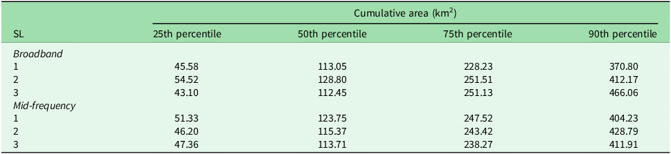
Dolphins were located throughout the study area and were not clustered within the localization array. There was no significant difference in the size of the kernel densities under different broadband (Fig. 1a–c & Table 1) or mid-frequency SLs (Table 1). There was a difference, however, in the spatial distributions of the dolphins in relation to ambient sound levels. Under broadband SL3, dolphins were found significantly farther east than under SL1 or SL2 (ANOVA: F2,287 = 13.31, p < 0.01). Dolphins were also found farther south under mid-frequency SL3 than in SL1 or SL2 (ANOVA: F2,287 = 13.67, p < 0.01). The Tukey-HSD test indicated that only the differences in spatial distribution between broadband SL1 and SL3 (3.50 km) and mid-frequency SL2 and SL3 (3.36 km) were larger than the median distances between localization results (3.28 km).
Plot of kernel densities for localizations of 100 randomly selected dolphin whistles (black circles) during (a) low (84.0–92.4 dBrms re 1 µPa; SL1), (b) medium (92.4–102.6 dBrms re 1 µPa; SL2) and (c) high (102.6–126.1 dBrms re 1 µPa; SL3) hourly broadband (10–7080 Hz) ambient sound levels, with the marine autonomous recording units (MARUs; white) and wind energy area (WEA; grey) shown. The 25th percentile (red) indicates the core 25% area of the dolphins’ locations. (d) The Maryland WEA (white) is displayed with the 100 randomly selected whistle localizations under high (102.6–126.1 dBrms re 1 µPa) broadband (10–7080 Hz) sound conditions, as well as the track densities of all vessels utilizing Automatic Identification Systems (AISs) in 2018 (MarineCadastre.gov, coast.noaa.gov/digitalcoast/data).

Figure 1. Long description
Panel A: A scatter plot with kernel density estimates showing the locations of 100 randomly selected dolphin whistles (black circles) during low hourly broadband ambient sound levels (84.0–92.4 dBrms re 1 µPa). The marine autonomous recording units (MARUs) are marked with white circles, and the wind energy area (WEA) is shown in grey. The 25th percentile (red) indicates the core 25% area of the dolphins’ locations. Panel B: A scatter plot with kernel density estimates showing the locations of 100 randomly selected dolphin whistles (black circles) during medium hourly broadband ambient sound levels (92.4–102.6 dBrms re 1 µPa). The MARUs are marked with white circles, and the WEA is shown in grey. The 25th percentile (red) indicates the core 25% area of the dolphins’ locations. Panel C: A scatter plot with kernel density estimates showing the locations of 100 randomly selected dolphin whistles (black circles) during high hourly broadband ambient sound levels (102.6–126.1 dBrms re 1 µPa). The MARUs are marked with white circles, and the WEA is shown in grey. The 25th percentile (red) indicates the core 25% area of the dolphins’ locations. Panel D: A scatter plot showing the Maryland WEA (white) with the 100 randomly selected whistle localizations under high broadband sound conditions (102.6–126.1 dBrms re 1 µPa), as well as the track densities of all vessels utilizing Automatic Identification Systems (AISs) in 2018.
Cumulative area (km2) for each percentile of the kernel density for the randomly selected whistles in each broadband (10–7080 Hz) and mid-frequency (2820–7080 Hz) sound-level category (SL).

Table 1. Long description
The table presents cumulative areas in square kilometers for different percentiles of kernel density for randomly selected dolphin whistles under various broadband and mid-frequency sound levels. It has 8 rows and 5 columns. The columns are labeled as 25th percentile, 50th percentile, 75th percentile, and 90th percentile under the heading Cumulative area (km2). The rows are labeled as SL 1, SL 2, and SL 3 under the headings Broadband and Mid-frequency. Row 1: Broadband SL 1, 45.58, 113.05, 228.23, 370.80. Row 2: Broadband SL 2, 54.52, 128.80, 251.51, 412.17. Row 3: Broadband SL 3, 43.10, 112.45, 251.13, 466.06. Row 4: Mid-frequency SL 1, 51.33, 123.75, 247.52, 404.23. Row 5: Mid-frequency SL 2, 46.20, 115.37, 243.42, 428.79. Row 6: Mid-frequency SL 3, 47.36, 113.71, 238.27, 411.91.
Dolphin movement patterns
Movement tracks (from 42 h total from 18 days) contained positions estimated from 643 dolphin whistles (Appendix S1 Table S1). Broadband sound levels for these hours ranged from 84.5 to 120.7 dBrms and mid-frequency sound levels ranged from 83.1 to 104.6 dBrms. Given the variability in location estimates for each whistle (approximately 3 km), the raw locations were all assigned an Argos location class of 0 in the SSM, which had an equivalent mean error (Costa et al. Reference Costa, Robinson, Arnould, Harrison, Simmons and Hassrick2010). SSM outputs with unrealistic dolphin travel speeds were removed (n = 42 locations), and this resulted in 35 tracks comprising 133 locations.
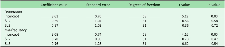
A linear mixed-effects model indicated that dolphin pod speeds were not significantly related to either broadband or mid-frequency ambient sound levels (Fig. 2b,c & Table 2). The straightness index also did not vary significantly in relation to broadband or mid-frequency sound levels (ANOVA: F2,22 = 0.53, p = 0.60, F2,22 = 0.01, p = 0.99, respectively; Fig. 2a & Table 2).
(a) All dolphin movement tracks within 15 km of the centre of the arrays that were used in the analysis (broadband sound level (SL)1: red, SL2: blue, SL3: green, beginning of the track: open black circle) and the Maryland wind energy area (WEA; yellow). Box plots of the dolphin pod speeds (m/s) and straightness indices (0 indicates a more circuitous path, 1 indicates a straight path) in relation to the (b,d) broadband (10–7080 Hz) and (c,e) mid-frequency (2820–7080 Hz) ambient SLs.

Results of the linear mixed-effects models for dolphin pod speeds in relation to the broadband (10–7080 Hz) or mid-frequency (2820–7080 Hz) ambient sound-level categories (SLs). The SL1 (lowest sound level) category was used as the reference level (Intercept) in each model.

Table 2. Long description
A table with two main sections: broadband and mid-frequency sound levels. Each section includes rows for intercept (SL1), SL2, and SL3. The table has five columns: Coefficient value, Standard error, Degrees of freedom, t-value, and p-value. Broadband section: Intercept row: Coefficient value 3.63, Standard error 0.70, Degrees of freedom 58, t-value 5.19, p-value 0.00. SL2 row: Coefficient value -0.59, Standard error 1.04, Degrees of freedom 31, t-value -0.56, p-value 0.58. SL3 row: Coefficient value 0.37, Standard error 1.03, Degrees of freedom 31, t-value 0.36, p-value 0.72. Mid-frequency section: Intercept row: Coefficient value 3.08, Standard error 0.74, Degrees of freedom 58, t-value 4.16, p-value 0.00. SL2 row: Coefficient value 0.70, Standard error 0.96, Degrees of freedom 31, t-value 0.73, p-value 0.47. SL3 row: Coefficient value 0.76, Standard error 1.23, Degrees of freedom 31, t-value 0.62, p-value 0.54.
Discussion
Using non-invasive methodologies for whistle localization and novel tracking and movement analyses, we found that bottlenose dolphins utilized different regions of this study area under elevated broadband and mid-frequency sound levels (Fig. 1). Our analyses indicated that dolphins did not, however, move at different speeds (Fig. 2b,c & Table 2), utilize more or less space (Table 2) or alter the directness of their travel (Fig. 2a,d,e) under different ambient sound conditions at these spatiotemporal scales.
In our study, dolphins were detected farther east (closer to the shipping lanes) under elevated sound conditions. While we were unable to determine the cause of this change, this could suggest that this habitat is preferable, perhaps because of altered prey distributions in the presence of large vessels (Ivanova et al. Reference Ivanova, Kessel, Espinoza, McLean, O’Neill and Landry2020). Alternatively, dolphins may be displaced to this more marginal habitat by an acoustic disturbance such as a vessel. Dolphins could also be clustering to maintain group cohesion, or other ecological drivers could be influencing their distribution. Additional research could investigate the presence of foraging, specific disturbances or whistle contributions to sound levels to better understand these drivers of distribution. Future studies could also collect data for a population consequences of disturbance model to indicate whether these altered habitat preferences affect the population dynamics of the animals in this region (Harwood et al. Reference Harwood, King, Schick, Donovan and Booth2014, Erbe et al. Reference Erbe, Dunlop, Dolman, Slabbekoorn, Dooling, Popper and Fay2018).
Because dolphins in this region are regularly exposed to elevated sound levels, the lack of change in dolphin pods’ speed and straightness of travel could be due to their resilience (New et al. Reference New, Harwood, Thomas, Donovan, Clark and Hastie2013) or habituation (Papale et al. Reference Papale, Azzolin and Giacoma2012) to those disturbances. Although much attention has been paid to physiological injury caused by sounds (e.g., Erbe et al. Reference Erbe, Dunlop, Dolman, Slabbekoorn, Dooling, Popper and Fay2018), behavioural effects are more common and more challenging to quantify. If dolphins ceased vocalizing during elevated sound levels (as in McCarthy et al. Reference McCarthy, Moretti, Thomas, DiMarzio, Morrissey and Jarvis2011), however, our understanding of their movements would be further limited with passive acoustic monitoring. Additionally, our approach did not account for the presence of dolphins that did not whistle, nor the presence of multiple pods of dolphins, and it could not easily distinguish between calls from different dolphins within a pod.
Similarly to other localization studies, the precision of this localization method significantly decreased as the dolphins’ distance from the array increased (Watkins & Schevill Reference Watkins and Schevill1972: 1 m error in a 100-m array; Zhang et al. Reference Zhang, Zeng, Gong and Zhao2016: 4 m error at 1000 m). Further refining the localization algorithm is recommended to provide precision appropriate for fast-moving, small cetacean species. While the SSM was utilized to account for both the challenges of localizing a pod of dolphins and to account for the level of imprecision in the CSE algorithm, it was designed for tracking the movement of a single, slow-moving individual. As a result, the SSM produced some locations that were deemed unreasonable given the known maximum speed of dolphin travel. The sampling rate of the recorders also resulted in clipping or missed higher-frequency whistles. Localizing individually identifiable calls such as signature whistles (Janik et al. Reference Janik, Sayigh and Wells2006) could allow the tracking of individuals to improve the reliability of metrics such as speed and directness of travel.
This study used novel methods of dolphin whistle localization and movement analysis to illustrate the habitat utilization of dolphins under varied sound levels and the non-lethal effects of acoustic disturbances on protected marine mammals. Altered spatial distributions, especially when exacerbated by changing ocean conditions, vessel traffic and other human activities, could lead to population-level disturbances (Harwood et al. Reference Harwood, King, Schick, Donovan and Booth2014, Erbe et al. Reference Erbe, Dunlop, Dolman, Slabbekoorn, Dooling, Popper and Fay2018). As vessel traffic and offshore energy development increase throughout this species’ range, acoustic disturbances will become more frequent and intense, and assessing the cumulative effects of these will become a critical priority for decision-makers.
Supplementary material
To view supplementary material for this article, please visit https://doi.org/10.1017/S0376892926100605.
Acknowledgements
Thanks to the crew from the Chesapeake Biological Laboratory and the crew from Cornell University for field assistance. Thanks to Slava Lyubchich for help with the statistical analyses and to Aimee Hoover for assisting with the ambient sound analyses.
Financial support
Project supported through a Cooperative Agreement with the Maryland Department of Natural Resources (MDNR), number 14-18-2420, with the assistance of the Maryland Offshore Wind Development Fund via the Maryland Energy Administration.
Competing interests
The authors declare none.
Ethical standards
Not applicable.
Disclaimer
The views and conclusions contained in this document are those of the authors and should not be interpreted as representing the opinions or policies of the US Government, the Maryland Department of Natural Resources or the Maryland Energy Administration. Mention of trade names or commercial products does not constitute their endorsement by the US Government or the state.




 Open access

