1 Introduction
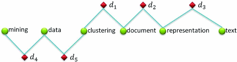
Representing documents as fixed-length vectors is necessary for many machine-learning tasks, such as document summarization, web search, and text analysis. The bag-of-words (BOW) model (Harris Reference Harris1954) is commonly used to represent documents in these domains because of its simplicity, efficiency, and good performance. However, BOW estimates the similarity between documents depending on the number of common words they share. Thus, BOW cannot identify the similarities between documents comprising different words. Figure 1 shows that, although all the five documents are semantically related, BOW cannot measure the relatedness between documents d 1 and d 4.
An example of the relations between documents, where the diamonds stand for documents and the circles stand for words. There is a link between a diamond and a circle if the corresponding word appears in the document.

To identify the semantic similarities between documents beyond how much they look alike, latent topic models are proposed, including Latent Semantic Indexing (Deerwester et al. Reference Deerwester, Dumais, Landauer, Furnas and Harshman1990), Latent Dirichlet Allocation (Blei, Ng and Jordan Reference Blei, Ng and Jordan2003), and doc2vec (Le and Mikolov Reference Le and Mikolov2014). With these methods, documents are represented as their distributions on numerous latent topics, and similar documents are supposed to have similar distributions on the topics. The expressive power of the topic models for document representation is remarkable. Nevertheless, the parameters, especially the dimensionality (number of topics), are often difficult to determine. Improper dimensionality would have distorted the original relations and added error (Landauer and Dumais Reference Landauer and Dumais1997).
Contrary to the latent semantic topics, statistical document enrichment methods (Rungsawang Reference Rungsawang1998; Billhardt, Borrajo and Maojo Reference Billhardt, Borrajo and Maojo2002; Kalogeratos and Likas Reference Kalogeratos and Likas2012; Cheng et al. Reference Cheng, Miao, Wang and Cao2013) construct the context of a document with the relatedness of all the words in the corpus to the document. The required relatedness is obtained according to statistical data, primarily the co-occurrence frequencies between words. As a result, the sparse document vector generated by BOW is enriched to be dense with the relatedness of the global words. The document enrichment methods do not have the limitation similar to the topic methods, i.e., a fixed dimensionality is determined by the number of distinct words in the dataset.
The classical document enrichment method is the Context Vector Model (Billhardt et al. Reference Billhardt, Borrajo and Maojo2002), CVM for short. For any document, CVM regards a word as related if it is related to any of the original words in the document. CVM considers two words as interrelated if they co-occur in the same document. In this sense, d 4 will be enriched with the context word ‘clustering’, because its original word ‘data’ has co-occurred with ‘clustering’ in d 5; d 1 will be enriched with the context word ‘data’ for the same reason. The generated document vectors of d 1 and d 4 will therefore have two words in common, and their relatedness can be identified. Nonetheless, the similarity between d 3 and d 4 remains unknown because they have no explicitly related words in common. The physical boundaries of documents hinder the evaluation of the relatedness between words.
To detect the latent relatedness between words which cannot be exploited through word co-occurrence frequencies, we infer the transitive-type relatedness between words according to their common explicitly related words, e.g., based on the relatedness scores between words A and B, and B and C, we estimate the relatedness between A and C. With this intuitive idea, the document vectors of d 3 and d 4 will have the words ‘clustering’ and ‘document’ in common, for ‘representation’ belonging to d 3 is related to ‘clustering’ via ‘document’ and ‘data’ belonging to d 4 is related to ‘document’ via ‘clustering.’ In this study, we restrict the relatedness of one word to another as the conditional probability that the word will co-occur along with the other. The probability view helps us theoretically infer the transitive relatedness. The relationship between the marginal probabilities of words and the conditional probabilities under the law of total probability regularizes the inference to avoid overestimation.
The proposed method has more smoothing power on generating the document vectors because more related words are used to enrich the spare BOW document vectors than the traditional document enrichment methods. Thorough evaluation on real datasets illustrates that significant improvement on document clustering has been achieved with the proposed method compared with state-of-the-art methods. In addition, as the document representation is improved by a better estimation of the relatedness between words, we have compared the generated word relatedness with human judgments. Comparative results on the three benchmark datasets, i.e., Rubenstein and Goodenough (Reference Rubenstein and Goodenough1965), Miller and Charles (Reference Miller and Charles1991), and WordSimilarity-353 (Finkelstein et al. Reference Finkelstein, Gabrilovich, Matias, Rivlin, Solan, Wolfman and Ruppin2002), also demonstrate the effectiveness of the proposed method. The contributions of this paper are as follows:
(1) We aim to tackle the critical issue of measuring the semantic similarities between documents. The intuitive idea is to infer the transitive relatedness between words to enrich the document vectors.
(2) We propose three strategies for measuring the transitive relatedness between words, which are derived by minimizing the differences between the marginal probabilities of the global words obtained with the law of total probability and those calculated by the raw frequencies.
(3) The experimental evaluation demonstrates that our approaches significantly improve the performance on document clustering compared with state-of-the-art methods on real datasets.
The remainder of this paper is organized as follows: Section 2 discusses previous work related to document enrichment methods. Section 3 provides preliminary related information. The novel methods are proposed in Section 4. The experimental results are presented in Section 5. Section 6 briefly discusses document representation and the future work. Section 7 concludes the paper.
2 Related work
The enrichment of sparse BOW document vectors has been done in previous studies. In accordance with the measures to estimate the relatedness of words to a document, the methods are divided into two groups. The statistical methods enrich document vectors with the relatedness computed with word co-occurrence frequencies. After counting the frequencies, some smoothing functions are used to re-weight the statistical results, e.g., Pseudo Conditional Probability (Billhardt et al. Reference Billhardt, Borrajo and Maojo2002), PCP for short, Positive Pointwise Mutual Information (Bullinaria and Levy Reference Bullinaria and Levy2007), PPMI for short, Term Frequency and Inverse Document Frequency (Iosif and Potamianos Reference Iosif and Potamianos2010), and Jaccard (Cheng et al. Reference Cheng, Miao, Wang and Cao2013). The concept behind these functions is that the word meanings should be independent of the corpus size and the word frequencies. The knowledge-based methods introduce external knowledge from dictionaries or ontologies (Gabrilovich and Markovitch Reference Gabrilovich and Markovitch2006; Hu et al. Reference Hu, Zhang, Lu, Park and Zhou2009; Wei et al. Reference Wei, Lu, Chang, Zhou and Bao2015). WordNet involved Document Representation method (AlAgha and Nafee Reference AlAgha and Nafee2016) enriches document representation with background knowledge from WordNet. Disambiguated Core Semantics method (Wei et al. Reference Wei, Wei and Yang2015) exploits lexical chains to extract the content of texts. Expert knowledge is more reliable than word co-occurrence frequencies. However, external resources usually tend to be mismatched or become out of date for a particular document collection.
As detailed in the following section, with the statistical document enrichment methods, word vectors consist of relatedness scores between words and document vectors are generated through the combination of word vectors. At present, the same idea is extensively used in the neural network domain. The input of these methods are the word vectors mapped into a low-dimensional space. Convolutional neural network for sentence modeling (Kim Reference Kim2014) combines the word vectors with the convolution kernels; Diversified Restricted Boltzmann Machine (Xie, Deng and Xing Reference Xie, Deng and Xing2015), DRBM for short, combines the word vectors with RBM; Word Mover’s Distance (Kusner et al. Reference Kusner, Sun, Kolkin and Weinberger2015), WMD for short, directly calculates the distances between documents according to the word vectors by reducing the issue to a special case of the well-studied Earth Movers Distance (Rubner, Tomasi and Guibas Reference Rubner, Tomasi and Guibas1998) transportation problem. We classify these methods as the topic models because of the low dimensionality. As previously discussed, determining the parameters is a challenge for these methods.
Although we focus on how to evaluate the relatedness between words, some other aspects of the statistical framework can be improved: the Semantic smoothing Vector Space kernel Method (Nasir et al. Reference Nasir, Varlamis, Karim and Tsatsaronis2013), S-VSM for short, avoids over enrichment by considering only the top-k semantically related terms; we propose the Deviated Document Enriching method (Wei, Wei and Yang Reference Wei, Wei and Yang2015), DDE for short, to combine word vectors by assigning different weights to each dimension.
3 Preliminaries
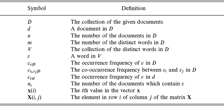
For simplicity, the notations to be used throughout this paper are listed in Table 1.
Definition of notations

With BOW, the m distinct words in the document collection D are used to construct the feature space. ∀d ∈ D, its document vector is represented as
 $$\begin{equation}
\Phi _{\mbox{bow}} : \mathbf {d} = (c_{v_1|d}, c_{v_2|d}, \ldots, c_{v_m|d})^T \in \mathbb {R}^{m}
\end{equation}$$
Considering that BOW cannot identify similar documents comprising different words, CVM is proposed to reveal the meanings of documents with a set of weighted word vectors.
∀v i ∈ V, its word vector is defined as Billhardt et al. (Reference Billhardt, Borrajo and Maojo2002), Turney and Pantel (Reference Turney and Pantel2010), Grefenstette et al. (Reference Grefenstette, Hermann, Dinu and Blunsom2014):
 $$\begin{equation}
\mathbf {v}_{i} = \left(\frac{c_{v_i,v_1|D}}{c_{v_i|D}}, \frac{c_{v_i,v_2|D}}{c_{v_i|D}}, \dots, \frac{c_{v_i,v_m|D}}{c_{v_i|D}}\right)^T
\end{equation}$$
Generally, the meanings of words should be independent of the corpus size. Therefore, the overall frequency of v i in the whole corpus, c vi|D, is introduced to present the basic context of v i (Bullinaria and Levy Reference Bullinaria and Levy2007). The values in vi measure the relatedness of the words in the vocabulary V to v i. In addition, if v j = v i, vi(j) = 1, implying that the relatedness of a word to itself is one.
Together with all the word vectors, an m × m matrix is obtained, i.e., V = (v1, v2, . . ., vm), which is called the context matrix. The document vector generated with CVM is
 $$\begin{equation}
\Phi _{\mbox{cvm}} : \mathbf {d}^{\prime} = \mathbf {Vd} = \sum _{i=1}^{m}{\mathbf {v}_i}\mathbf {d}(i) \in \mathbb {R}^{m}
\end{equation}$$
where the document vector of d is enriched with the average relatedness of all the words in V to the original words in d. The essential part of the framework is the estimation of the relatedness between words. Equation (2) shows that the relatedness between words depends on their explicit co-occurrence frequencies in the entire corpus, where it is defined as the explicit relatedness between words. As discussed with Figure 1, the physical boundaries hinder the enrichment process to find all the related words to a document, specifically, to the original words of the document.
Similar to our intuition, the Coupled term-term Relation Model (CRM) (Cheng et al. Reference Cheng, Miao, Wang and Cao2013) has implemented the idea of inferring the transitive relatedness. Equation (4) displays the details of CRM where |L| denotes the number of the common related words in  $L=\lbrace v_k|\frac{c_{v_i,v_k|D}}{c_{v_i|D}}>0 \wedge \frac{c_{v_j,v_k|D}}{c_{v_j|D}}>0\rbrace$, and α is an empirical parameter that remains the same for all the words. Clearly, the strength of the transitive relatedness between any two words is the accumulation of the weaker strengths of their explicit relatedness to the common related words. The transitive relatedness between words is defined as the implicit relatedness. The final relatedness, which is called the complete relatedness, is the accumulation of the explicit and implicit relatedness scores with the empirical parameter α.
 $$
\begin{eqnarray}
\mathbf {v}_i(j)= \left\lbrace \begin{array}{@{}l@{\quad}l@{}}\alpha \frac{c_{v_i,v_j|D}}{c_{v_i|D}} + \frac{(1-\alpha)}{|L|}\sum _{v_k\in L}\min _{a=i,j}\lbrace \frac{c_{v_a,v_k|D}}{c_{v_a|D}}\rbrace & j \ne i\\
1& \mbox{else} \end{array}\right.
\end{eqnarray}$$
As the implicit relatedness extends the definition of the relatedness between words, inter-unrelated words will be regarded as related to each other if they co-occur with the same word, which is likely to happen because almost all the words have co-occurred with the stop words, e.g., ‘is’, ‘the’, and ‘a’. The explicit relatedness becomes necessary to regulate the overestimated implicit relatedness. However, the relations between the explicit and implicit relatedness scores of different pairs of words are difficult to control using a single parameter. CRM has the risk of reducing the discriminativeness of the generated document vectors with over weight to the implicit relatedness. A better strategy is therefore needed.
4 Total probability model
The previous sections presented the advantages of using the implicit relatedness between words to enrich a document. However, an effective strategy for quantifying the implicit relatedness or for strategy combining the explicit and implicit relatedness has not been developed. Instead of separately calculating the explicit and implicit relatedness scores, we directly compute the complete relatedness through the explicit relatedness.
Equation (2) shows that, ∀v i, v j ∈ V; the explicit relatedness of v j to v i could be regarded as the conditional probability that v j will appear when v i occurs. That is,
 $$\begin{equation}
\frac{c_{v_i,v_j|D}}{c_{v_i|D}}=P(v_j|v_i)
\end{equation}$$
The probability view provides the theoretical foundation to infer the implicit relatedness and to find the relation between the complete relatedness and the marginal probabilities of words, which are explained in detail below. We can then automatically estimate the weights of the explicit and implicit relatedness scores through linear regression by referring to the marginal probabilities.
4.1 Definition of the complete relatedness
We assume that the conditional probability of one word under the occurrence of another could be corrected according to their current distributions on all the words in V with proper weights for each word.
Definition 1
∀v i, v j ∈ V, the complete relatedness of v j to v i is defined as
 $$\begin{equation}
P^{\prime}(v_j|v_i)=\frac{\sum _{k=1}^m \omega _k P(v_i|v_k)P(v_j|v_k)P(v_k)}{P(v_i)}
\end{equation}$$
where the parameters ωk, k = 1, . . ., m, are the weights of the words in V.
Definition 1 is derived by considering the following two factors:
(1) As
 $P(v_j|v_i)=\frac{P(v_i,v_j)}{P(v_i)}$, re-estimating the conditional probability is equivalent to re-evaluating the joint probability P(v i, v j). Supposing ∀v i, v j ∈ V, v i and v j are independent of each other, we have
(7)With the law of total probability,Footnote 1 we further obtain$$\begin{equation}
P(v_i,v_j|v_k)=P(v_i|v_k)P(v_j|v_k)
\end{equation}$$
(8)which means the joint probability could be derived from the joint probabilities of the co-occurrences of v i and v j with each of the m distinct words. However, the independency assumption cannot hold in most cases. With respect to the dependencies between words, i.e.,$$\begin{equation}
P(v_i,v_j)=\sum _{k=1}^m P(v_i,v_j,v_k) = \sum _{k=1}^m P(v_i,v_j|v_k)P(v_k)=\sum _{k=1}^m P(v_i|v_k)P(v_j|v_k)P(v_k)
\end{equation}$$
(9)and$$\begin{equation}
P(v_i,v_j|v_k)\ge P(v_i|v_k)P(v_j|v_k)
\end{equation}$$
(10)we can only infer that P(vi, vj) ≃ ∑mk = 1P(vi|vk)P(vj|vk)P(vk).$$\begin{equation}
P(v_i,v_j) \le \sum _{k=1}^m P(v_i,v_j,v_k)
\end{equation}$$
(2) As the deviations between the left and right sides of Equations (9) and (10) are both related to the words v k (k = 1, . . ., m), we introduce the parameters ωk to smoothen the potential conflict incurred by the dependencies between words to make Equation (8) hold
(11)The introduced parameters imply that the co-occurrence between v i and v j under the occurrence of v k in Equation (9) mainly depends on their relatedness to v k, ωk can handle the dependencies of the joint probabilities in Equation (10). Essentially, ωk is a parameter of v k.$$\begin{equation}
P(v_i,v_j) = \sum _{k=1}^m \omega _kP(v_i|v_k)P(v_j|v_k)P(v_k)
\end{equation}$$


Dividing P(v i) from both sides of Equation (11), we obtain Definition 1.
From the semantic view, P(v i|v k) and P(v j|v k) are the explicit relatedness of v i to v k and v j to v k, respectively. Instead of selecting the smaller value between P(v i|v k) and P(v j|v k), the relative implicit relatedness between v i and v j via v k is defined as P(v i|v k)P(v j|v k)P(v k), which is approximately equal to the joint probability among v i, v j, and v k.
Furthermore, as P(v i|v i) = 1, when v k = v i, we have
 $$\begin{equation*}
\frac{P(v_i|v_i)P(v_j|v_i)P(v_i)}{P(v_i)}=\frac{P(v_j|v_i)P(v_i)}{P(v_i)}=P(v_j|v_i)
\end{equation*}$$
which is the explicit relatedness of v j to v i. Similarly, when v k = v j,  $\frac{P(v_i|v_j)P(v_j|v_j)P(j)}{P(v_i)}$ also equals P(v j|v i). Thus, the defined conditional probability is just the complete relatedness, which combines the explicit and implicit relatedness with the parameters ωk (k = 1, . . ., m).
Instead of empirically presetting the parameters, the optimization method for solving them will be presented in the following section, which significantly distinguishes the proposed method from CRM.
4.2 Estimation of the parameters
4.2.1 Estimation through the marginal probabilities
For convenience, we organize the parameters and the marginal probabilities in the vector form ω = (ω1, ω2, . . ., ωm)T and p = (P(v 1), P(v 2), . . ., P(vm))T, respectively. Supposing ω is known, with the law of total probability, we can obtain
 $$\begin{equation}
\forall v_i\in V, P(v_i)= \sum _{k=1}^m \omega _k P(v_i,v_k) = \sum _{k=1}^m \omega _k P(v_i|v_k)P(v_k)
\end{equation}$$
where the parameters in ω vanish the conflicts caused by the dependencies of the joint probabilities as claimed above.
By extending p to an m × m matrix P where P = (p, . . ., p), Equation (12) is equivalent to the following expression:
 $$\begin{equation}
\left(\mathbf {V}\cdot \mathbf {P}^T\right) \bm {\omega}=\mathbf {p}
\end{equation}$$
where Xa × b · Ya × b is the dot product of two matrices, which returns an a × b matrix with the value in row i of column j equivalent to X(i, j)Y(i, j). Let A = V · PT, the element in row i of column k of A is the joint probability P(v i, v k).
Based on Equation (13), estimating the parameters is equivalent to minimizing the objective function as follows:
 $$\begin{equation}
O=\Vert \mathbf {A}\bm {\omega}-\mathbf {p} \Vert ^2
\end{equation}$$
The analytical solution of Equation (14) is
 $$\begin{equation}
\bm {\omega}=\left(\mathbf {A}^T\mathbf {A}\right)^{-1}\mathbf {A}^T\mathbf {p}
\end{equation}$$
Equation (15) presents a solution to estimate the parameters ωk by referring to the marginal probabilities of all the words according to Equation (12). Equation (12) claims the ground truth that the marginal probability of v i should be equal to the sum of the conditional probabilities of v i under the occurrences of all the words.
4.2.2 Estimation through the constant restriction
P(v i) could also be derived from the conditional probabilities of all the words under the occurrence of v i:
 $$\begin{equation}
\forall v_i\in V, P(v_i)= \sum _{k=1}^m \omega _k P(v_i,v_k) = \sum _{k=1}^m \omega _k P(v_k|v_i)P(v_i)
\end{equation}$$
Dividing P(v i) from both sides of the equation, we have
 $$\begin{equation}
\forall v_i\in V,\sum _{k=1}^m \omega _k P(v_k|v_i)=1
\end{equation}$$
Similar to Equations (12), Equation (17) has the following equivalent expression:
 $$\begin{equation}
\mathbf {V}^T \bm {\omega}=\mathbf {1}
\end{equation}$$
where 1 is a m × 1 vector with all the values equivalent to one. The objective function for estimating the parameters in ω becomes
 $$\begin{equation}
O=\Vert \mathbf {V}^T\bm {\omega}-\mathbf {1} \Vert ^2
\end{equation}$$
Thus, the parameters are given by
 $$\begin{equation}
\bm {\omega}=\left(\mathbf {V}\mathbf {V}^T\right)^{-1}\mathbf {V}\mathbf {1}
\end{equation}$$
Equation (20) provides another solution of ω by referring to the constant value one.
4.2.3 Estimation through the semantic consistency
We have presented two solutions of ω, which are both derived from the constraints implied by the law of total probability. In accordance with previous works (Billhardt et al. Reference Billhardt, Borrajo and Maojo2002; Cheng et al. Reference Cheng, Miao, Wang and Cao2013),  $P(v_i|v_i)=\frac{P(v_i,v_i)}{P(v_i)}$ should equal one, that is, P(v i, v i) = P(v i). By substituting Equation (8) into the equation, we have
 $$\begin{equation}
P(v_i,v_i)= \sum _{k=1}^m \omega _k P(v_i|v_k)P(v_i|v_k)P(v_k) = P(v_i)
\end{equation}$$
Equation (21) is equivalent to the following vector form:
 $$\begin{equation}
\left(\mathbf {P}^T \cdot \mathbf {V}\cdot \mathbf {V}\right) \bm {\omega}=\mathbf {p}
\end{equation}$$
Let A = PT · V · V, estimating the weights will minimize the objective function as
 $$\begin{equation}
O=\Vert \mathbf {A}\bm {\omega}-\mathbf {p} \Vert ^2
\end{equation}$$
where the element in row i of column k of A is the joint probability P(v i, v i, v k).
The analytical solution of the objective function is
 $$\begin{equation}
\bm {\omega}=\left(\mathbf {A}^T\mathbf {A}\right)^{-1}\mathbf {A}^T\mathbf {p}
\end{equation}$$
Equation (21) shows that this solution estimates the parameters by referring to the marginal probabilities of all the words similar to Equation (15). While this solution follows the semantic constraint that the relatedness of a word to itself is one rather than the constraint derived from the law of total probability which Equation (15) obeys. With this solution, the joint probability of the co-occurrence between a word and itself keeps consistently equal to its marginal probability.
4.3 Implementation of the proposed method
We have proposed three solutions to estimate ω. For all the three methods, we must construct the context matrix V first. For both Equations (15) and (24), we need the marginal probabilities of the words as the reference to estimate ω. With the obtained ω, we compute the complete relatedness and generate the enriched document vectors. These steps are detailed in this section.
To construct the context matrix, we should estimate the explicit relatedness between words. For a fair comparison with CVM, we take PCP. Besides, among other candidate methods (Mihalcea, Corley and Strapparava Reference Mihalcea, Corley and Strapparava2006), we take PPMI and LIN (Lin Reference Lin1998). PPMI is reported to achieve the best performance on word semantic similarity estimation among the statistical methods (Bullinaria and Levy Reference Bullinaria and Levy2007; Wei and Wei Reference Wei and Wei2013). LIN is a well-known knowledge-based method which measures the pairwise relatedness between words with WordNet. Incorporated with LIN, the proposed method becomes a hybrid of statistical and knowledge-based methods. Details of PCP, PPMI, and LIN are illustrated below:
1. PCP
(25)where r(v i, v j) denotes the explicit relatedness between v i and v j.$$\begin{equation}
r(v_i,v_j)=\sum _{a=1}^{n}{\displaystyle \frac{c_{v_i|d_a}}{\sum _{k=1}^m c_{v_k|d_a}}\cdot \displaystyle \frac{c_{v_j|d_a}}{\sum _{k=1}^m c_{v_k|d_a}}}
\end{equation}$$
2. PPMI
(26)where$$
\begin{eqnarray}
r(v_i,v_j)= \left\lbrace \begin{array}{@{}l@{\quad}l@{}}log_2\frac{P(v_i,v_j)}{P(v_i)P(v_j)} & P(v_i,v_j) > P(v_i)P(v_j)\\
0& P(v_i,v_j) \le P(v_i)P(v_j) \end{array}\right.
\end{eqnarray}$$
$P(v_i,v_j)=\frac{c_{v_j,v_i|D}}{\sum _{i=1}^{m}\sum _{j=1}^{m}c_{v_i,v_j|D}}$ $P(v_i)=\frac{c_{v_i|D}}{\sum _{j=1}^{m}c_{v_j|D}}$. We implement PPMI with the reported optimal parameter (Bullinaria and Levy Reference Bullinaria and Levy2007; Wei and Wei Reference Wei and Wei2013), i.e., the context window size of 2. Restricting the context window size to 2 means only when one word appears next to another, they are regarded as co-occurred.3. LIN
(27)where c i is the corresponding concept of v i in the WordNet taxonomy, IC(c i) = −log2P(v i), and ICS(c i, c j) is the least common subsumer in the taxonomy.$$\begin{equation}
r(v_i,v_j)= \frac{2\text{IC}(\text{LCS}(c_i,c_j))}{\text{IC}(c_i)+\text{IC}(c_j)}
\end{equation}$$


With respect to Equation (5), the explicit relatedness computed with any of the above methods is normalized to conditional probability, that is,
 $$\begin{equation}
P(v_j|v_i)=\frac{c_{v_i,v_j|D}}{c_{v_i|D}}=\frac{r(v_i,v_j)}{\sum _{j=1,j\ne i}^m r(v_i,v_j)}
\end{equation}$$
Note that P(v j|v i) = 1 when i = j.
Generally, we assume that the occurrence frequencies of the words are sufficient to generate reliable marginal probabilities. To make the assertion more plausible, we introduce the threshold TH to verify whether the occurrence frequency of a word is sufficient. Without loss of generality, suppose the words in V are organized in descending order according to their occurrence frequencies, and ∀i ⩽ t, c vi|D > TH; ∀i > t, c vi|D ⩽ TH. The estimation of the marginal probabilities incorporated with the threshold is given as follows:
 $$\begin{equation}
\forall v_i \in V, P(v_i) = \left\lbrace \begin{array}{@{}l@{\quad}l@{}}\displaystyle \frac{c_{v_i|D}}{\sum _{j=1}^m c_{v_j|D}} & i\le t\\
[14pt] \displaystyle \frac{\sum _{j=t+1}^m c_{v_j|D}}{(m-t)\sum _{j=1}^m c_{v_j|D}}&\text{else} \end{array}\right.
\end{equation}$$
The words with the occurrence frequencies less or equal to the threshold are regarded as less frequent words. Equation (29) gives the less frequent words the same marginal probability.
Furthermore, we set the weights of the less frequent words at one. As the weights are introduced to smoothen the conflicts incurred by the dependencies between words and the less frequent words always co-occur with some specific words which have low dependencies with others, the conflicts incurred by the less frequent words must be small. In addition, if two words are related to some less frequent word, they are likely to be interrelated, for the less frequent word expresses some specific meaning generally, which has more power to link the two words. Thus, we prefer the less frequent words, and give them more weights. Consequently,
 $$\begin{equation}
\bm {\omega}=[\bm {\omega}_1,\bm {\omega}_2]^T
\end{equation}$$
where ω1 = (ω1, . . ., ωt) and  $\bm {\omega}_2=(\underbrace{1, \dots, 1}_{m-t})$.
Similarly, let
 $$\begin{equation}
\mathbf {A}=[\mathbf {A}_1, \mathbf {A}_2]
\end{equation}$$
where A1 is an m × t matrix with A1(i, 1: t) = A(i, 1: t), and A2 is an m × (m − t) matrix with A2(i, 1: (m − t)) = A(i, (t + 1): m).
The calculation of w1 is
 $$\begin{equation}
\bm {\omega}_1=\left(\mathbf {A}_1^T\mathbf {A}_1\right)^{-1}\mathbf {A}_1^T(\mathbf {p}-\mathbf {A}_2\bm {\omega}_2)
\end{equation}$$
A2ω2 returns an m × 1 vector with the ith element equal to ∑mk = t + 1ωkP(vi, vk). As p(i) = P(vi) = ∑mk = 1ωkP(vi, vk), the ith element in p − A2ω2 equals ∑tk = 1ωkP(vi, vk). That is, by setting the weights of the less frequent words to one, p − A2ω2 returns the marginal probabilities of all the m distinct words without considering their co-occurrences with the less frequent words.
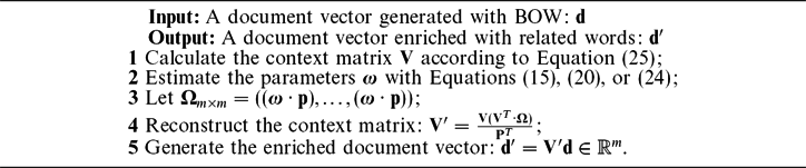
The generating process of document vectors is concluded as Algorithm 1. Step 4 calculates the complete relatedness between words defined by Equation (6), and Step 5 generates the enriched document vector according to Equation (3), where the context matrix is replaced with the matrix V′ fulfilled with the complete relatedness.
Document Vector Generating with TPM

With respect to the generating process, it costs Θ(m 2) times to calculate all the complete relatedness between words, and Θ(mn) times to calculate the relatedness of each word to the given n documents. Floating space amounting to m × m and m × n are needed to store the context matrix and the enriched document vectors, respectively. As the number of words is limited in practice, the complexity of calculating the relatedness between words has an upper bound. The overall time and space to be consumed is max{Θ(m 2), Θ(mn)}.
The proposed method is called the Total Probability Model (TPM), because the law of total probability is used to bridge the gap between the conditional probabilities and the constraints used by all the three equations for the acquisition of ω. For distinction, the version incorporated with Equation (15) is named as TPMF because the ‘frequencies’ of each word are the criteria to follow when estimating ω; the version incorporated with Equation (20) is called TPMO because the constant value ‘one’ is the target to approach; the version incorporated with Equation (24) is referred to as TPMS because the ‘semantic constraint’ is followed by the target function. The differences among the objective functions significantly distinguish the proposed solutions. Together with the three methods to estimate the explicit relatedness between words, we can get nine subversions of TPM: TPMF-PCP, TPMF-PPMI, TPMF-LIN, TPMO-PCP, TPMO-PPMI, TPMO-LIN, TPMS-PCP, TPMS-PPMI, and TPMS-LIN, respectively.
5 Experiments
In the experimental part, we evaluate the proposed methods on two tasks: one is document clustering to illustrate the representation power of the proposed method; the other is word semantic similarity estimation to verify the accuracy of the defined complete relatedness. For each task, we compare TPM with the topic models, the knowledge-based document enrichment methods and the traditional statistical document enrichment methods, respectively. Through the thorough evaluation, we show the progress that TPM makes compared with the traditional statistical methods and the overall performance of TPM compared with state-of-the-art methods. In addition, to verify the effect of TH, we conduct the experiments with different values of TH. The detailed results are shown in the parameter selecting section.
5.1 Document clustering
5.1.1 Experimental setup
Dataset. In this section, we conduct the performance evaluation using the TDT2 and Reuters datasets.Footnote 2 The TDT2 dataset consists of data extracted from six sources, including two newswires (APW, NYT), two radio programs (VOA, PRI), and two television programs (CNN, ABC). Those documents appearing in two or more categories are removed, and the categories with more than ten documents are kept, thus leaving us with 10,021 documents in total. The Reuters dataset contains 21,578 documents which are grouped into 135 classes. Those documents with multiple category labels are discarded, and the categories with more than ten documents are selected. This leaves us with 8,213 documents in total. Table 2 provides the statistics of the datasets.
Clustering Algorithm. The performance of the pairwise similarity evaluation is an important criterion to verify the qualities of the representations for documents. Generally, with good representation, the similarities between semantically related documents should obtain high scores, while the similarities between unrelated documents should obtain low scores. This is consistent with the purpose of the clustering task that similar documents are organized into the same group, while dissimilar documents are organized into different groups. Therefore, we evaluate our algorithms on document clustering problem with the k-means clustering algorithm. The cosine of document vectors is chosen to be the similarity measure. The evaluation of the similarities between documents directly affects the results of k-means, thus can reflect the qualities of the representation methods for documents.
Evaluation Metrics. Two metrics are adopted to evaluate the performance of document clustering, the Accuracy (AC) (Xu, Liu and Gong Reference Xu, Liu and Gong2003) and the Normalized Mutual Information (NMI) (Andrews and Fox Reference Andrews and Fox2007). Given a document vector da, let r a and l a be the cluster label and the label provided by the document collection, respectively, AC is defined as follows:
(33)where n denotes the total number of documents in the test, δ(l a, map(r a)) is the delta function that equals one if l a = map(r a) and equals zero otherwise, and map(r a) is the mapping function that maps each cluster r a to the equivalent label from the document collection. The best mapping can be found by using the Kuhn–Munkres algorithm (Lovász and Plummer Reference Lovász and Plummer1986).$$\begin{equation}
\mbox{AC} = \frac{\sum _{a=1}^n \delta (l_a,\text{map}(r_a))}{n}
\end{equation}$$
Let n l be the number of documents in class l, n r be the number of samples in cluster r, and n l, r be the number of samples in class l and cluster r, then
(34)$$\begin{equation}
\mbox{NMI} = \frac{\sum _{l,r}n_{l,r}\text{log}\frac{nn_{l,r}}{n_l n_r}}{\sqrt{(\sum _l n_l \text{log}\frac{n_l}{n})(\sum _r n_r \text{log}\frac{n_r}{n})}}
\end{equation}$$
It is easy to check that NMI ranges from 0 to 1. Since the cluster number is predefined as the number of the classes in the document collection, NMI = 1 if cluster r is identical to class l, and NMI = 0 if the two sets are independent.
Evaluation Baselines. The document representation methods to be compared include the following:
(1) The popular BOW method is used as the baseline.
(2) The topic models including the well-known LDA, doc2vec, and the recently proposed WMD and DRBM are compared. The Non-negative Matrix Factorization based document representation (Xu et al. Reference Xu, Liu and Gong2003) and Locally Consistent Concept Factorization (Cai, He and Han Reference Cai, He and Han2011) are also compared, for they were once tested with the above corpora on the same task.
(3) The knowledge-based document enrichment methods, i.e., WordNet involved Document Representation and Disambiguated Core Semantics are compared.
(4) CVM, S-VSM, and CRM, which belong to the statistical branch, are performed to verify the improvement of TPM.
With respect to the referred methods, the frequencies of words in each document are smoothed with the tf-idf weighting schemeFootnote 3 if the document vectors generated with BOW are required. For doc2vec, the context window parameter is selected from 1 to 50 in steps of 1 and the dimension parameter is chosen from 50 to 300 in steps of 10. The best results are obtained with the context window of 39 and the dimension of 300. For the other methods, the recommended values for their specific parameters reported in the papers are used.


Statistics of the datasets

5.1.2 Performance evaluations
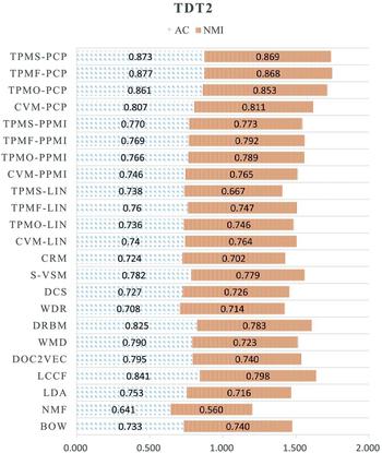
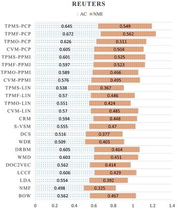
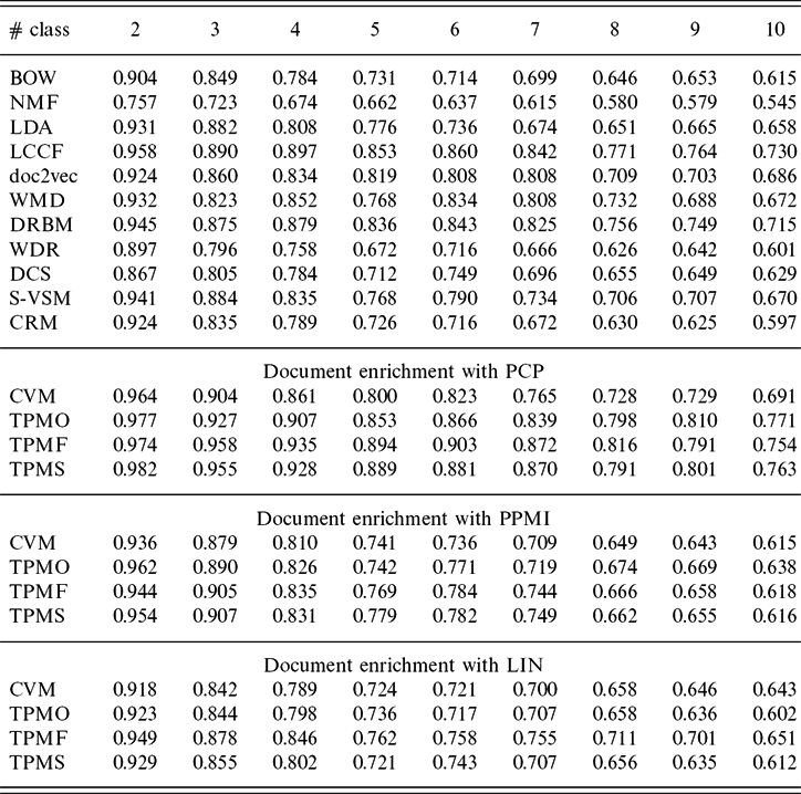
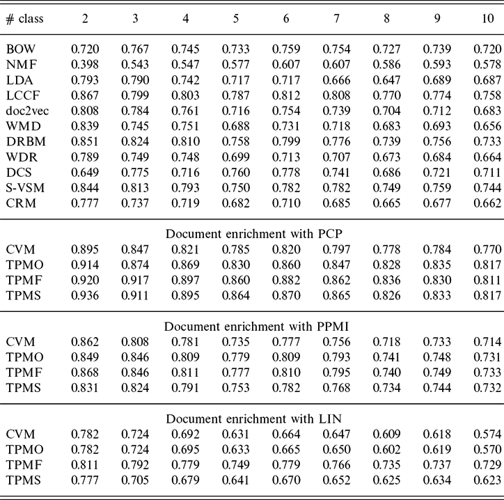
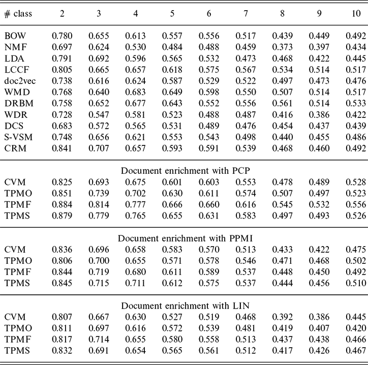
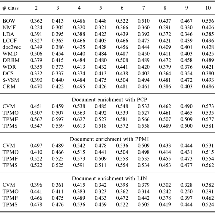
For both TDT2 and Reuters, the class number is set from 2 to 10. For each given class number, fifty test runs were performed on different randomly chosen classes. Hence, the evaluation was conducted on 900 different datasets actually. TPMF is test with TH = 1.78 × 10⁻⁴ on both datasets. While TPMS is performed with TH = 1.07 × 10⁻³ on TDT2, and TH = 7.13 × 10⁻⁵ on Reuters. The average performances of the methods are shown in Figures 2 and 3. The average performances for each class number are reported in Tables A1–A4 of Appendix A. According to the results, TPMF incorporated with PCP performs best. It achieves 6.5% performance improvement on TDT2 compared with Locally Consistent Concept Factorization, the best of the other methods; it achieves 11.2% performance improvement on Reuters compared with CVM, the best of the other methods. These experiments reveal a number of interesting points:
(1) CVM performs better than BOW. This illustrates the superiority of enriching documents with related words.
(2) TPM incorporated with PCP and PPMI achieves more significant improvements than CVM. Since CVM only considers the explicit relatedness between words, the further improvements achieved by TPM indicate the necessity of breaking through the physical boundaries of word co-occurrences and utilizing the implicit relatedness between words to find more related words.
(3) The uncompetitive performance of CRM demonstrates that the inaccurate evaluation of the complete relatedness over enriches the generated document vectors. The proposed strategy is proved to be effective by regularizing the inference of the complete relatedness into the framework of the law of total probability. In this sense, the proposed methods have more enriching power than the other statistical methods on document representation.
(4) TPMF and TPMS outperform TPMO. The distribution of the marginal probabilities of words must imply some innate semantic information which promotes the performances of TPMF and TPMS. The detailed performances shown in Tables 4– 7 demonstrate that TPMF performs slightly better than TPMS on different clustering tasks with the variant class numbers.
(5) Largely due to the low coverage of WordNet, the knowledge-based methods are not competitive with BOW including the proposed TPM method incorporated with LIN. There are about 11.5% of the words in Reuters and 19.1% of the words in TDT2 are not covered by WordNet. Although we can infer the implicit relatedness with TPM, the context matrix is too sparse to support the estimation based on the distribution of the explicit relatedness between words. For both datasets, the ratio of the non-zero values in the context matrix is less than 20%. Besides, the polysemy of words hinders the estimation of the relatedness between words. With the statistical methods, the relatedness between words is expected to be the common sense in the given document collection. While ontologies are independent of the document collection. The quantified relatedness is possibly inconsistent with the common sense, and is not applicable to most documents.
(6) In most cases, the results of the proposed methods are better than the topic models. The topic models extract the latent topics implied by the document collection and assign the documents to these topics, which incurs the issue of determining the number of topics. In particular, the worse performance of the topic methods with NMI test may attribute to the less number of predefined topics, which forces the documents belonging to different topics assigned to the same predefined topic (NMI tests the purity of each cluster).
Average clustering results on TDT2.

Average clustering results on Reuters.

5.2 Word semantic similarity
5.2.1 Experimental setup
Evaluation datasets. The word semantic similarity evaluation is conducted on three standard datasets that have been widely used in the past:
(1) Rubenstein and Goodenough (RG-65) consists of sixty-five word pairs ranging from synonymy pairs (e.g., car – automobile) to completely unrelated terms (e.g., noon – string). The sixty-five noun pairs were annotated by fifty-one human subjects. All the noun pairs are scored using a scale from 0 (not-related) to 4 (perfect synonymy).
(2) Miller and Charles (MC-30) is a subset of RG-65, consisting of thirty word pairs. The similarity of each word pair was rated by thirty-eight human subjects, using a scale from 0 to 4.
(3) WordSimilarity-353 (WS-353), also known as Finkelstein-353, consists of 353 word pairs annotated by 13–16 human experts, on a scale from 0 (unrelated) to 10 (very closely related or identical). MC-30 is a subset in WS-353. Unlike MC-30, which consists only of generic words, WS-353 also includes proper names and technical terms, therefore posing an additional degree of difficulty for statistical based methods (topic models and statistical methods).
Evaluation metric. Following prior literatures (Gabrilovich and Markovitch Reference Gabrilovich and Markovitch2007; Hassan and Mihalcea Reference Hassan and Mihalcea2011), we compute Spearman’s rank order correlation coefficient between the algorithm’s predictions and the average human judgments on each dataset. Spearman’s correlation coefficient is considered to be much more robust than Pearson’s linear correlation.
Baseline methods. The proposed methods are compared with several state-of-the-art systems: the traditional statistical methods, namely PCP and PPMI, the topic models including Latent Semantic Analysis (Landauer et al. Reference Landauer, Laham, Rehder and Schreiner1997) and word2vec (the skip-model version) (Mikolov et al. Reference Mikolov, Sutskever, Chen, Corrado and Dean2013), and the knowledge-based methods, i.e., LIN, Explicit Semantic Analysis (Gabrilovich and Markovitch Reference Gabrilovich and Markovitch2007), and Multi-Prototype Word Representation (Wu and Giles Reference Wu and Giles2015).
The results of Latent Semantic Analysis, LIN, and Explicit Semantic Analysis are shown in the state of the art Wiki page of the Association for Computational Linguistics,Footnote 4 mostly extracted from Hassan and Mihalcea (Reference Hassan and Mihalcea2011); the results of word2vec are reported in Wang, Mohamed and Hirst (Reference Wang, Mohamed and Hirst2015); the results of Multi-Prototype Word Representation are directly obtained from the authors.
Setup of the proposed methods. The English Wikipedia corpusFootnote 5 is used as the statistical base. The downloaded file is the 2016-11-28 version, which is about 13.5 GB size with total 17,069,180 articles. To filter out noises and truncate the feature space to computable size, a common trick is to remove stop and rare words (Lebret and Collobert Reference Lebret and Collobert2015). Following this idea, we have filtered out the most frequent 350 words, removed the words co-occurred with none of the words in the test data, limited the feature space to 10,000 dimensions. The reserved words are those with frequencies ranging from 4.837 × 10⁻⁷ to 1.216 × 10⁻³.
When it comes to evaluating the semantic similarity between words, the proposed methods are split on how to utilize the complete relatedness. With reference to the traditional statistical methods, for any two words, the single explicit relatedness between them is lack of confidence, hence their similarity is estimated according to the similarity between the contexts comprising their explicit relatedness to all the words, that is, the cosine similarity between their word vectors. Similarly, the proposed complete relatedness is obtained by considering the overall explicit relatedness, it should be sufficient to measure the semantic similarities between words. Besides, the cosine similarity is equivalent to the dot product of two normalized vectors. The complete relatedness is also the result of the dot product of word vectors composed by explicit relatedness. So we simply take the complete relatedness defined in Equation (11) as the final semantic similarity score. On the other hand, we can generate new word vectors comprising complete relatedness according to Algorithm 1 and take the cosine similarity of the new word vectors as the semantic similarity score. We denote the semantic similarity calculated by the former as CTPMF, CTPMO, and CTPMS, respectively, and denote the semantic similarity calculated by the latter as FTPMF, FTPMO, and FTPMS, respectively. As the context matrix comprising the explicit relatedness between words measured with LIN is too sparse to infer the implicit relatedness, only the versions of TPM incorporated with PCP and PPMI are tested.
5.2.2 Performance evaluations
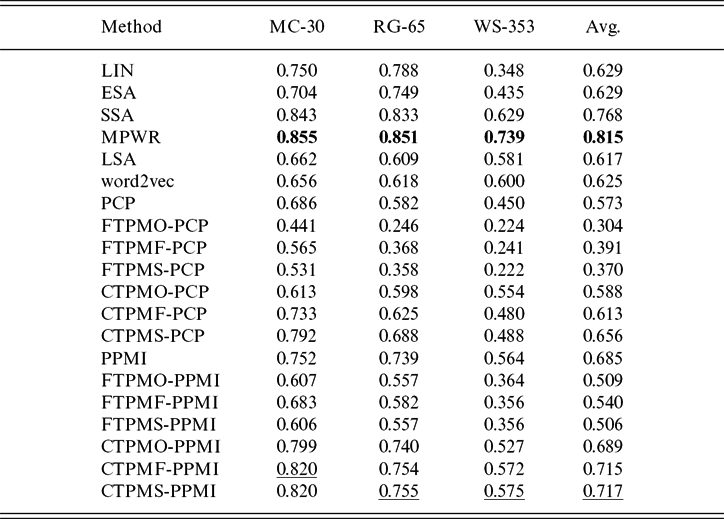
The Spearman’s correlation coefficients between the algorithm’s predictions and the average human judgments on the three datasets are presented in Table 3, where the bold values are the state-of-the-art best scores, and the underlined values are the best scores achieved with the proposed methods. For CTPMF and FTPMF, the results on MC-30, RG-65, and WS-353 are obtained with TH equivalent to 2.70 × 10⁻⁵, 1.27 × 10⁻⁴, and 2.26 × 10⁻⁵, respectively, for CTPMS and FTPMS, the results are obtained with TH equal to 1.27 × 10⁻⁴, 1.27 × 10⁻⁴, and 9.51 × 10⁻⁶. The following conclusions are derived from the results:
(1) The results show that CTPMF, CTPMO, and CTPMS outperform the statistical methods and topic models. More specifically, CTPMF-PPMI has achieved the best results. CTPMF, CTPMO, and CTPMS incorporated with PPMI have achieved 4.4 per cent, 0.6 per cent, and 4.7 per cent performance improvements compared to PPMI, respectively. As both the cosine similarity and the complete relatedness are the dot product between word vectors, they calculate the similarity score by counting the matching degree along each dimension of the word vectors. The cosine similarity treats the dimensions equivalently, while the complete relatedness distinguishes the importance of each dimension through the introduced ω parameters and the marginal probabilities. The superiority of the proposed methods demonstrates the effectiveness of introduced mechanism.
(2) CTPMF and CTPMS perform better than CTPMO by incorporating with the distribution of the marginal probabilities, which is consistent with the document clustering results.
(3) CTPMF, CTPMO, and CTPMS are not as effective as the knowledge-based methods, especially on WS-353. The polysemy, synonym, and semantic changing phenomena of words increase the difficulty for the statistical methods to detect the semantic similarities between the proper names and technical terms in WS-353.
(4) FTPMF, FTPMO, and FTPMS have not made any progress compared with PCP or PPMI. This result agrees with the prior work (Lebret and Collobert Reference Lebret and Collobert2015) which argues that the similarity between words is better expressed with syntactic related words rather than with semantic related words. Too many semantically related words occur in the word vectors used for the computation of similarity scores.
Spearman correlations on word semantic similarity datasets

5.3 Parameter selection
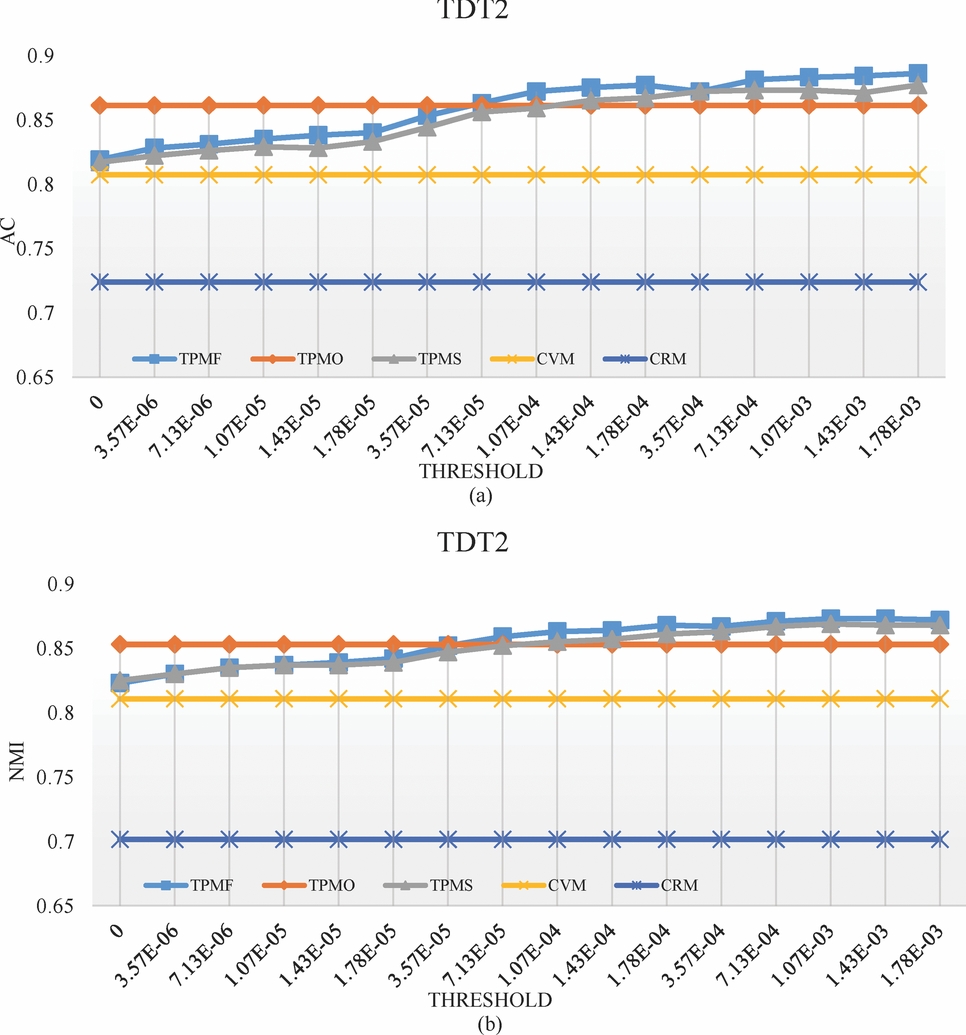
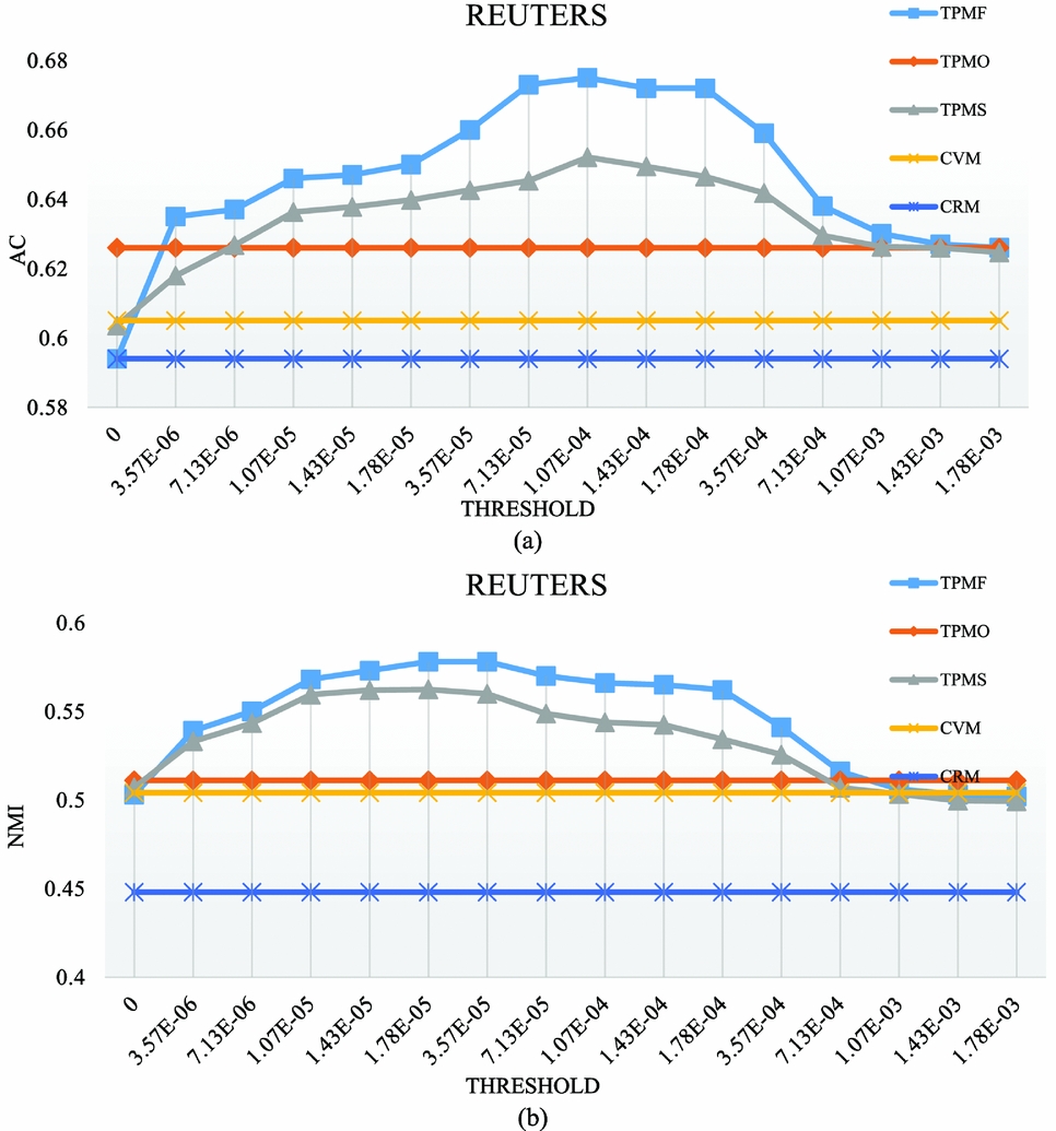
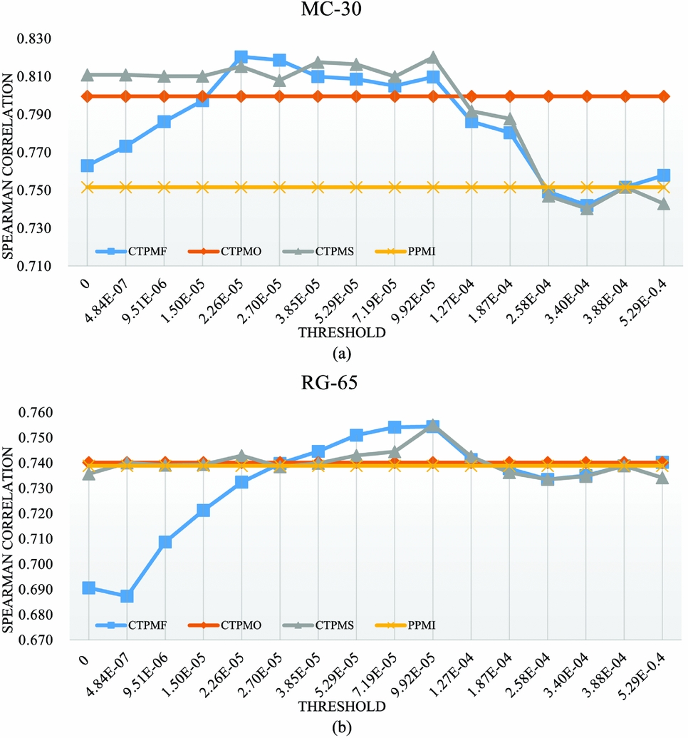
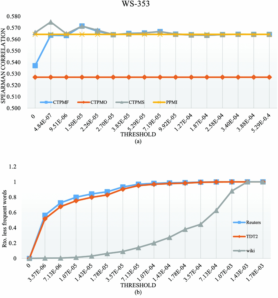
TH is essential to TPMF and TPMS. Figures 4–7 show how the performances of TPMF and TPMS vary with the values of TH. PCP and PPMI are chosen for document clustering and word semantic similarity evaluation, respectively, for they achieve the best results on each task. The horizontal axis is the value of TH and the vertical axis denotes the corresponding performances. The figures show that TPMF and TPMS achieve consistent better performances than CVM or CRM with the values of TH ranging from 3.57 × 10⁻⁶ to 7.13 × 10−04; TPMF and TPMS (specifically, CTPMF and CTPMS) obtain better results than PPMI in most cases. Thus, we can choose the value of TH in a wide range.
The performances of the proposed methods with the different values of TH on TDT2.

The performances of the proposed methods with the different values of TH on Reuters.

The performances of the proposed methods with the different values of TH on MC-30 and RG-65.

The performances of the proposed methods with the different values of TH on WS-353 and the proportions of the reserved marginal probabilities with the different values of TH.

As the introduction of the marginal probabilities makes the performances of TPMF and TPMS partially depend on the sufficiency of the occurrence frequencies, unreliable marginal probabilities of words, especially those corresponding to low frequencies, may lead TPM to unexpected results. The experimental results demonstrate that omitting unreliable marginal probabilities through tuning TH is effective on inferring the complete relatedness. However, we lack clear guidelines for judging which marginal probabilities are unreliable, excessive removal of marginal probabilities is at the expense of losing the implied semantic information of the marginal probabilities that the performance of TPM will decrease. The choice of TH is to strike a balance between the reliability of the marginal probabilities and the amount of the implied semantic information.
Empirically, the optimal results of TPMF and TPMS on TDT2 and Reuters are obtained when TH is taken around 10−4, while on the Wiki corpus, the preferable TH is around 10−5. According to Figure 7, TH with these scores omit about ninety per cent of the marginal probabilities on TDT2 and Reuters, but only twenty per cent on Wikipedia. This reveals the common sense that the reliability depends on the size of the corpus. As Wikipedia is much larger than TDT2 or Reuters, the marginal probabilities are more statistically reliable.
Although the semantic similarity evaluations on MC-30, RG-65, and WS-353 are performed on the same Wiki corpus, TH causes variant effects on them. As the ω parameters are the global optimal values based on all the word vectors, they cannot always be the best for the subset of word vectors required by a particular test set. As a result, the performances of TPMF and TPMS with the same TH vary on different test sets.
All in all, the marginal probabilities of words not only imply some semantic information but also bring about the uncertainty about the reliability of marginal probabilities. TPMO obtains stable performance by giving up the semantic information, while TPMF and TPMS achieve more significant performance improvements at the risk of performance uncertainty. The choice of TH is to strike a balance between the reliability of the marginal probabilities and the amount of the implied semantic information, which mainly depends on the size of corpus. The empirical values for small corpora, e.g., TDT2 and Reuters, are around 10−4 and around 10−5 for huge corpora like Wikipedia.
6 Discussion and future work
In the previous section, we have evaluated the performances of the topic models, the knowledge-based methods and the statistical methods on different tasks independently. We proceed by discussing their performances in the following.
Recent years, the topic models, especially the Neural Network Models (NNM) have become a research hotspot. Various neural network architectures (Le and Mikolov Reference Le and Mikolov2014; Rui et al. Reference Rui, Liu, Yang, Li, Zhou and Li2015; Amiri and III Reference Amiri and III2016) have been proposed to represent document in the low-dimensional space. NNMs have been incorporated to produce promising results in many supervised NLP tasks, while they have played a more minor role in unsupervised learning problems (Das, Zaheer and Dyer Reference Das, Zaheer and Dyer2015). In our test, NNM have not performed good enough on both the document clustering and the semantic similarity evaluation tasks. We attribute the less promising results of NNMs in unsupervised tasks to the mixture of informations: NNM embeds not only the semantic information but also the syntactic information into the document vectors (Mitchell and Steedman Reference Mitchell and Steedman2015). The unnecessary information could be filter out through supervised training but may disturb the performance of unsupervised calculations. In addition, unsupervised criteria are possibly less informative to train the millions of parameters. In this sense, the relations between word co-occurrence frequencies and occurrence frequencies adopted by TPMF and TPMS are new semantic constraints, adding them to NNMs (e.g., adding the criteria to the cost function of doc2vec) has the potential to generate better results.
The knowledge-based methods have achieved the best results on semantic similarity evaluation, but much worse on document clustering. According to our analysis, the coverage of an ontology limits the performance of the knowledge-based methods. On the contrary, the proposed method has the best results on document clustering, while not so good on semantic similarity evaluation. The statistical methods are not good at identifying the exact relations between proper names and technology terms. Therefore, it is worth attempting the integration of the knowledge-based methods and the proposed method to enhance word relatedness estimation and to tackle the coverage issue with the proposed implicit relatedness inference mechanism. According to our experiment, for this extension, it is preferred to use more abundant knowledge base than WordNet or involve the statistical methods at the step of explicit relatedness estimation. The polysemy issue also need to be handled before inferring the implicit relatedness based on the knowledge-based methods.
7 Conclusion
This study proposes a novel document representation model called TPM to measure the semantic relatedness between documents. In order to find more related words to a document, TPM leverages the implicit relatedness between words, which breaks through the limitations caused by the physical boundaries of word co-occurrences. The implicit relatedness is calculated by considering all the common explicitly related words to the pair of words. To avoid overestimation, the contribution of each common related word to the implicit relatedness is weighted using an optimization framework based on the law of total probability, according to which TPM is extended to three subversions, namely, TPMF, TPMO, and TPMS. The effectiveness of TPM has been verified by comparison with the explicit relatedness, cosine similarity between word vectors and CRM. As a result, TPM has achieved state-of-the-art performance on document clustering and comparative results on word semantic similarity evaluation.
TPMF and TPMS perform better than TPMO. The significant difference between TPMF, TPMS, and TPMO is that TPMF and TPMS estimate the implicit relatedness by referring to the marginal probabilities of words, which is thought to imply some semantic information. The performances of TPMF and TPMS depend on a parameter, which is determined by the size of corpus. A proper value for the parameter is a balance between the reliability of the marginal probabilities and the amount of the implied semantic information.
Appendix: Detailed clustering results
Clustering results on the TDT2 dataset (AC)

Clustering results on the TDT2 dataset (NMI)

Clustering results on the Reuters dataset (AC)

Clustering results on the Reuters dataset (NMI)