INTRODUCTION
Are exchange rates really random walks? It is well known that the proportion of exchange rate fluctuations that current economic models can predict is essentially zero. This fact was first noticed by Meese and Rogoff (1983a,b, 1988), who found that a random walk model forecasts exchange rates better than economic models.1
Meese and Rogoff compared out-of-sample forecasts, which are forecasts constructed on the basis of actual (future) values of the explanatory variables, rather than forecast values of the explanatory variables. Rolling forecasts are forecasts made on the basis of the most recent fraction of the observations available in the sample size. Thus, in order to make a rolling forecast, one has to re-estimate (i.e., update the estimate of) the parameter vector for every forecast.
An alternative explanation of this puzzling evidence is the presence of parameter instability. In fact, parameter stability is desirable in order to obtain good forecasts. Recent research by Stock and Watson (1996, 1999, 2003) finds convincing evidence that parameter instability is a widespread phenomenon in the empirical analysis of time series data, especially in monetary aggregates and interest rates. The result is robust to different choices of tests and the good forecasting ability of some economic variables seems to be casual across time periods and across countries.
The contribution of this paper is to address the problem of model selection between economic models of exchange rate determination and the random walk in the presence of parameter instability. Tests for model selection fail to detect parameter instability, and tests for parameter instability are not designed to choose between nested models. Out-of-sample tests, instead, are a robust method for choosing between two models in the presence of parameter instability. However, if the issue is to test whether exchange rates are random walks, then one could use optimal tests along the lines proposed by Rossi (2005), which provides optimal tests for nested model selection in the presence of parameter instability. The optimal tests jointly test for both parameter instability and a null hypothesis on the parameters and apply to situations in which one is interested not only in whether the explanatory variables proposed by some economic model are statistically significant in explaining the observed data, but also in whether this relationship is stable over time.2
Of course, forecasting tests are useful even if both models are mis-specified and are powerful in detecting more general forms of mis-specification than those addressed in this paper. Thus, it must be kept in mind that the tests proposed in this paper are useful within the model selection context for which they are designed.
This paper provides empirical evidence on parameter instability in models of nominal exchange rate determination. Interestingly, for some currencies, optimal tests that are robust to parameter instability do reject the hypothesis that the random walk is the best description of the data. This would explain why, although economic models exploit the information contained in other economic series, they nevertheless do not forecast better than a random walk. We also explore whether it is possible to improve forecasts by explicitly taking into account the presence of parameter instability. For this purpose, we compute forecasts both of a random walk time-varying parameter model [as in Stock and Watson (1996)] and of Elliott's (2005) forecast combination method in the presence of a single break. We find that, in some cases, taking time variation in the parameters into account is capable of improving forecasts relative to the random walk.
In a recent and very much related paper, Clark and McCracken (2005) have also discussed the issue of the relationship between model selection and forecasting in the presence of parameter instability. They too note that in-sample predictive ability need not imply out-of-sample predictive ability, and the cases in which they differ may be explained by the presence of parameter instability. In fact, they examine the power properties of out-of-sample tests relative to Granger causality tests and conclude that out-of-sample predictive ability is harder to find because it depends on the timing of the structural break, whereas in-sample Granger causality is easily found if predictive ability exists in any portion of the sample. Their empirical results on interest rate spreads and stock prices for GDP growth nicely complement the results in this paper, showing that structural breaks can account for out-of-sample forecasting failure in other economic situations. It should also be stressed that the use of in-sample and out-of-sample tests have different goals. Out-of-sample tests are likely to be useful in situations where the researcher is interested in comparing forecasting ability and dynamic mis-specification may be allowed under both the null and the alternative hypothesis [see Corradi and Swanson (2004, 2005) and Chao et al. (2001)]. In-sample tests such as those used in this paper may shed light on the causes of poor out-of-sample forecasting ability of economic models. Another related paper is Inoue and Kilian (2002), which analyzes instead the relationship between forecasting and information criteria in the possible presence of structural breaks.
This paper is organized as follows. The next section discusses the motivation of the paper, Section 3 presents the tests considered in this paper, Section 4 presents the empirical results, Section 5 explores whether time-variation in the parameter can be used for forecasting, and Section 6 concludes.
MOTIVATION
The question of whether existing models of nominal exchange rate determination are a good description of the empirical data is of considerable practical and policy interest. Notwithstanding the huge literature, reviewed by Frankel and Rose (1995) and Meese (1990), the issue is far from settled, although the prevailing view is that the answer is No. A related problem of models of nominal exchange rate determination is their embarrassingly poor forecasting ability in out-of-sample forecasting experiments, especially relative to the random walk model (see Meese & Rogoff, 1983a,b). In fact, the random walk model is not an economic model and, thus, it is worrisome that it forecasts better than economic models. The question addressed in this paper, then, is whether the presence of parameter instability can explain the poor out-of-sample forecasts of the economic models.
To be concrete, let a researcher be interested in testing whether the exchange rate is a random walk (and thus its rate of growth, call it x1,t, is unpredictable) against the possibility that x1,t can be explained by the lagged values of the rates of growth of some fundamentals, x2,t−1. For example, Meese and Rogoff (1988) consider the real interest rate parity condition (RIPC),3
The reason that the example is in terms of real exchange rates whereas the rest of the paper is about nominal exchange rates is the following. Meese and Rogoff (1988) contains an illuminating discussion about why out-of-sample tests are used rather than in-sample tests, and it is nicely linked to parameter instability. This provides an intuitive motivation for this paper. However, the most famous Meese and Rogoff puzzle deals with nominal exchange rates, so the present paper is about nominal exchange rates.

where εt is unforecastable, Model 1 is the random walk, and Model 2 is the economic model (the RIPC in this example).
Testing in-sample whether the exchange rate in levels is a random walk, then, implies testing whether β equals zero versus the alternative that the parameters are different from zero (recall that x1,t is the rate of growth of the exchange rate, so that if β = 0 then the rate of growth is unpredictable and, thus, the exchange rate in levels is a random walk). An in-sample likelihood ratio test could then be used. But if the test does not reject the null hypothesis, so that β is not significantly different from zero, can we conclude that the random walk is really the best description of the data?
Looking more carefully into Meese and Rogoff's (1988) results, we find overwhelming evidence of parameter instability. In fact, a Chow test for a structural break at the time of the Reagan election widely rejects the null hypothesis of no structural break [see Meese and Rogoff (1988, Table II)]. Motivated by the presence of parameter instability, Meese and Rogoff (1988) conclude that the in-sample tests are not reliable, and instead use out-of-sample forecast comparisons. In fact, it is commonly argued that out-of-sample tests are robust to the presence of parameter instability, as the parameters are re-estimated over time. The out-of-sample forecast comparison, however, still turns out to favor the random walk. In no case do the economic models do better than the random walk in terms of point forecasts, and the random walk is significantly better in some cases. The same results occur in Meese and Rogoff (1983a,b).
However, since the data suggest that the relationship between the real exchange rate and the fundamentals is very unstable over time, the true comparison that the researcher should be making is between the following two models:

where the notation βt emphasizes that the parameter is time-varying. Thus, the random walk model really imposes two restrictions, namely that the parameters are constant over time (βt = β*, say) and that they equal zero (β* = 0). Rossi (2005) proposes an in-sample test for this joint hypothesis that has optimal properties and that can be used in this context. The next section describes this test more in detail, along with the other tests used in this paper to shed some light on the relationship between exchange rates and fundamentals.
THE TESTS CONSIDERED IN THIS PAPER
In this paper, we are concerned about testing a hypothesis on a parameter vector as well as about testing parameter instability. When the alternative hypothesis of interest is either the former or the latter, then optimal tests are available. In the latter case, optimal tests for parameter instability that can be used when the break date is unknown are the tests proposed by Andrews and Ploberger (1994), Andrews (1993) and Nyblom (1989). In the former case, a Likelihood Ratio test on the parameter vector is optimal.
However, when both hypotheses are of interest, considering tests for parameter instability and Likelihood Ratio tests separately is not sufficient any more. Out-of-sample tests have been used in the empirical literature to deal with the problem of testing whether a given theoretical model is a good description of the observed data when there is an underlying problem of parameter instability. These tests can be robust to parameter instability because they use rolling or sequential methods to estimate the parameters recursively. They also can detect model mis-specification because they compare the average squared forecast error of the unrestricted model with that of the restricted model.
Even if out-of-sample tests can potentially detect both model mis-specification and parameter instability, their asymptotic local power is not the highest for the joint null hypothesis of interest. Rossi (2005), instead, identifies a class of tests that are optimal, in the sense of having the highest asymptotic local power against both parameter instability and a null hypothesis on the parameters.
In this paper we will thus consider the following tests, each of which focuses on a well-specified null hypothesis discussed here below. Let β be the parameter vector, and let βj denote a subset of the parameters.
A. Likelihood Ratio Test (LR): βj = 0 for Some (or all) Parameters (forgetting about possible time variation in the parameters)
If all the coefficients are statistically insignificantly different from zero then the fundamentals are not good explanatory variables for the exchange rate. The LR test is the main model specification test usually considered in the literature for comparing nested models. The p-values are obtained by the asymptotic distribution of the test, which is
, where p (the numbers of degrees of freedom) corresponds to the number of restrictions.4
p-values are obtained by linear interpolation from existing tables.
B. Tests for Time-Varying Parameters (TVP test): βtj Constant Over Time (i.e., , for Some constant but unknown and unspecified) not for Some (or all) βtj
The tests for time-varying parameters are the Quandt (1960) Likelihood Ratio (QLR) test developed by Andrews (1993), denoted by QLRT, the Andrews and Ploberger (1994) Exponential-Wald and Mean-Wald tests, respectively denoted by Exp-WT and Mean-WT, and the Nyblom (1989) test, denoted by NyblomT. The p-values reported for these tests are obtained by linear interpolation from a simulation of 5,000 Monte Carlo replications over a dense grid.
C. Optimal Tests for Model Specification and Time-Varying Parameters: βtj = 0 for Some (or all) βtj
These tests are the optimal tests discussed in Rossi (2005): the optimal Andrews and Ploberger (1994) Exponential and Mean Wald tests, Exp-W
and Mean-W
, the optimal Andrews QLR test, denoted by QLR
, and the optimal Nyblom (1989) test, denoted by Nyblom
. The p-values reported for these tests are obtained by linear interpolation from a simulation of 5,000 Monte Carlo replications over a dense grid.
D. Out-of-Sample Tests: E (MSFEm-MSFErw)= 0
Out-of-sample (hereafter oos) tests are constructed in two stages. In the first stage, the parameters of the model are estimated in a fraction of the sample; in the second stage, the estimates are used to forecast the value of the dependent variable (the nominal exchange rate) one period ahead into the future in the remaining part of the sample. To evaluate the relative forecasting performance of two models, we use their mean square forecast errors (MSFE). The MSFE is the average of the squares of the difference between the forecast and the true value of the dependent variable over the forecasting sample. This paper focuses on whether the fundamentals (plus the constant and possibly lagged values of the dependent variable) are useful predictive variables for the dependent variable. Hence, the test compares the MSFE of the unrestricted estimated model (MSFEm) to the MSFE of the restricted model under the null hypothesis that all (or a subset of) the coefficients are equal to zero (MSFErw). The out-of-sample tests considered here are the Diebold and Mariano (1995) test and the Clark and McCracken (2001) ENC-NEW test, denoted respectively by DMT and ENCT. The first one is provided here because it is commonly used in the literature, but it is not appropriate in our case because the models are nested [see McCracken (1999) and Clark and McCracken (2001)]. The ENC-NEW test is designed specifically for nested models. Depending on whether the parameters are (i) estimated only once and then held fixed for all subsequent forecasts, (ii) estimated recursively by using all the available data at the time of the forecast, or (iii) estimated recursively by using only the most recent observations, the out-of-sample tests will be called (i) split, (ii) recursive, or (iii) rolling. The p-values reported for the DMT test are obtained by noting that, according to Diebold and Mariano (1995), the squared statistic is asymptotically
. However, unless very special circumstances occur (e.g., the fraction of the sample used for forecast validation is very small relative to the fraction used for parameter estimation), the correct test statistic when models are nested is ENCT; because the ENCT test has nonstandard critical values [see Clark and McCracken (2001)], we do not report its p-value but instead use a superscript to denote whether it is significant at conventional (10%, 5%, and 1%) critical values.5
Note that the Diebold and Mariano test does not take parameter estimation error into account, whereas West (1996) does. We do not report the latter, as its validity, like that of the Diebold and Mariano's test, is restricted to non-nested models. There are many other “out-of-sample” tests, such as those of Chao et al. (2001) and Corradi and Swanson (2004), that are not investigated here.
THE EMPIRICAL APPLICATION TO MODELS OF NOMINAL EXCHANGE RATES
We use monthly data from Datastream, from March 1973 to December 1998 [results for the subsample considered by Meese and Rogoff (1983a), that is, from March 1973 to June 1981, lead to similar conclusions]. The model is the simple monetary model considered by Meese and Rogoff (1983a). It explains the bilateral nominal exchange rate fluctuations between two countries by the difference between their real outputs, nominal money supplies, and nominal short-term interest rates. All the variables have stochastic trends (according to the Phillips–Perron test for unit root). To ensure stationarity, we will consider the rate of growth of these variables, calculated as first differences of logarithms. In particular, the regression functions considered involve the following variables: (a) the first difference of the logarithm of the bilateral, end-of-period nominal exchange rate; the bilateral exchange rates considered are those of Canada, France, Germany, Italy, and Japan versus the United States; (b) the first difference of the logarithms of the money (and output) ratios of the two countries considered, with the convention that the US variable is in the denominator; (c) the first difference of the difference between contemporaneous short-term interest rates of each country relative to the United States.
Let us introduce some notation in order to describe the models considered in this section. Let et denote the rate of growth of the nominal exchange rate, mt denote the rate of growth of the money ratio, yt denote the rate of growth of the real output ratio, and it denote the first difference of the difference between the two countries' nominal, short-term interest rates. Let us call “fundamentals” all the variables (in growth rates) that, according to the monetary model, are explanatory variables for the exchange rate, that is, mt, yt, and it collectively considered.
In this paper we consider the relationship between the nominal exchange rate and lagged fundamentals. This is different from Meese and Rogoff (1983a), who analyzed the relationship between the nominal exchange rate and contemporaneous fundamentals, but closer in spirit to Stock and Watson (2003) and the recent forecasting literature [Clark and McCracken (2005)]. The regressions are the following:


where the parameters are possibly time-varying and thus are indexed by t. The models AR(1) and AR(2) are univariate, respectively first- and second-order, autoregressive models for the rate of growth of the nominal exchange rate. The models ARX(1) and ARX(2) (where “X” means that the autoregression is augmented with exogenous variables) analyze the relationship between the rate of growth of the exchange rate and the rate of growth of its lagged fundamentals, adding also lagged values of the dependent variable in order to deal with possible serial correlation of the error term. The first considers only one lag, the second two lags. Since there is empirical evidence that exchange rates are conditionally heteroskedastic, all tests use robust estimates of covariance matrices.
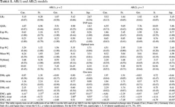
Table 1 shows the results for the autoregressive models. According to the LRT test, the lagged values are significant in some cases. Overall, there is no evidence of parameter instability and the optimal tests do not reject the random walk model even if, in some instances, the out-of-sample ENCT tests find that the random walk model forecasts significantly better than the autoregressive models.

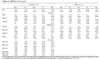
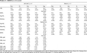
Tables 2 and 3 show the results for the ARX(1) and ARX(2) models. Notice that the in-sample Likelihood Ratio test, LRT, here compares the economic model with the random walk (because the exchange rate is in first difference). For most currencies, the likelihood ratio test does not reject the null hypothesis that all the parameters in the model are jointly equal to zero at the 5% significance level, especially if only one lag is selected. That is, this test does not reject the random walk model. Independent tests for parameter instability find some evidence of parameter instability, especially if one considers the ARX(2) model or the QLR test. So the economic model should have poor forecasting ability and, in fact, the out-of-sample rolling test results show that the economic model's forecasts are not better than those of the random walk, and sometimes significantly worse. However, the optimal tests reject the random walk model for some currencies at the 10% significance level for the ARX(1) model and especially for the ARX(2) model. This means that, even if in sample the random walk model is not rejected, the random walk model is not a good description of the data.


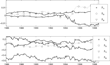
However, notice also that, when the optimal tests reject the null hypothesis, this does not mean that the economic model is a better description of the data than the random walk. It is only possible to conclude that there is some relationship between the exchange rate and its fundamentals, but it is not stable over time. This is especially evident if one looks at the optimal tests on fundamentals only, reported in the right panel of the tables, which compare the ARX(1) and ARX(2) economic models with, respectively, univariate autoregressive processes of order one and two for the exchange rate. The results uncover the time-varying relationship and attribute it to the relationship between the fundamentals and the exchange rate. The temporal evolution of the parameter values on lagged fundamentals for the ARX(2) case (estimated recursively on a rolling window of about half of the sample size) is depicted in Figure 1. Similar, unreported tests on the parameters on the lagged exchange rate only do not find evidence of a time-varying relationship.

In conclusion, the empirical analysis shows that there does not seem to be a stable Granger causality relationship between the rate of growth of the exchange rate and its fundamentals, and this shows up in bad forecasts if one uses economic models to infer future values of the exchange rate. In general, the oos tests show that the economic model does not deliver significantly better forecasts than the simple random walk model (or the univariate autoregressive models). However, in some cases, the optimal tests do reject the null hypothesis that the random walk is a better description of the data than the economic model, and these cases correspond to situations in which there is parameter instability in the data.
FORECASTING IN THE PRESENCE OF TIME-VARYING PARAMETERS
In the previous section, we found that there does not seem to be a stable relationship between the exchange rate and the fundamentals. An interesting question is then whether it is possible to improve the out-of-sample forecasting performance of the monetary model by using time-varying parameter estimation techniques. Existing results in the literature show that regime-switching models are still unable to beat a random walk [cf. Engel (1994) and Marsh (2000)], whereas time-varying parameter models have been shown to outperform the random walk [cf. Wolff (1987) and Schinasi and Swamy (1989)]. Additional evidence comes from Wright (2004), who finds that combining models' information may, in some circumstances, provide better forecasts than a random walk. As discussed in Timmermann (in press), one of the possible reasons that forecast combinations work is the presence of structural breaks. Related to this point, Elliott (2005) proposes a new forecast combination method that explicitly takes into account the presence of parameter breaks.
In what follows, we will thus consider whether taking into account the possibility that parameters may be time-varying or the existence of possible breaks in the parameters is capable of improving forecasts relative to the random walk. As in Stock and Watson (1996), we will consider a random walk coefficient time-varying parameter model with various degree of coefficient evolution [see also Stock and Watson (1998)],

where ηt ∼ iid(0, λ2σ2Q), E(ηtεt) = 0 ∀t, k, and
. We estimate the model by using the Kalman filter, initializing the models by using a diffuse prior (β0 = 0 and a state covariance matrix set to vI where v is large). Also, as in Stock and Watson (1996), we consider various possible values for λ (0.0025, 0.005, 0.0075, 0.01, 0.015, 0.02) and select both the value of λ and the lag length (for a maximum lag length of 2) that maximizes the conditional predictive least-squares criterion.6
We checked the robustness of the results to a larger grid of values for λ.
We also consider Elliott's (2005) method, which explicitly takes into account the existence of breaks in the forecasting procedure. Because the time of the break is unknown, he proposes to compute forecasts at every possible break date, and then average them by using some weighting function. The weighting functions considered here are either equal weights, or weights such as those proposed by Andrews and Ploberger (1994), which are smallest for each end of the sample and largest in the center.
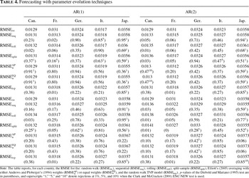
The results are reported in Table 4. The table reports, for each country, the root mean squared forecast error (RMSE) of the random walk (RMSErw) along with those of the sequential, rolling, and split-sample recursive estimation techniques (respectively labeled RMSEseq, RMSEroll, RMSEsplit), that of Elliott's (2005) averaging technique [with either Andrews and Ploberger's (1994) weights, labeled RMSE
, or equal weights, labeled RMSE
], and that of the random walk TVP model (labeled RMSEtvp). In parentheses, we report p-values of the Diebold and Mariano (1995) test for equal predictive ability, and superscripts 1, 5, and 10 denote rejections at 1%, 5%, and 10% when the Clark and McCracken (2001) ENC-NEW test is used. In this exercise we consider the AR(1), AR(2), ARX(1), and ARX(2) models described in Section 4 for all the estimation methods above except for the random walk TVP model, whose specification and lag length are recursively chosen over time according to the conditional predictive least-squares criterion.

A few interesting conclusions emerge from the analysis. While, overall, the random walk still performs better than the other estimation procedures, still the random walk TVP estimation method is better for Japan in all models, and Elliott's (2005) method is at least as good or even outperforms it for Canada, Germany, and Japan in the AR(1) case, and Japan in the AR(2) case. However, this difference is rarely statistically significant according to the Diebold and Mariano (1995) test, although it is sometimes significant if one uses Clark and McCracken's (2001) ENC-NEW statistic (which is more appropriate because the models are nested). We thus conclude that methods that estimate the evolution of the parameters over time have some room for improvement over a random walk, especially for the Japanese data.
CONCLUSIONS
Two models can be compared from the point of view of their in-sample fit or from their forecasting performance. It is quite common, especially in empirical international finance, that even if models fit reasonably well in sample, their forecasting performance is disappointing. Since Meese and Rogoff (1983a,b), many authors have documented that it is challenging to explain exchange rate fluctuations with macroeconomic fundamentals: a random walk model forecasts future exchange rates better than existing macroeconomic models. Are the economic models useless then?
Interestingly, Meese and Rogoff (1988) also noticed the presence of widespread parameter instability. This justifies their forecast-based model comparisons based on rolling out-of-sample tests, which continuously update the estimates of the parameters. This paper revisits the problem of comparing the monetary model of nominal exchange rate determination with the random walk in the presence of parameter instability. In some cases, even if out-of-sample tests do not reject the hypothesis that the random walk forecasts better, the optimal tests do reject the hypothesis that the random walk is the best description of the data. However, this does not mean that the economic model is a better description of the data than the random walk. In fact, these situations correspond to those in which there is parameter instability in the data. This raises the possibility that, by carefully investigating the nature of parameter instability and exploiting it, it may be possible to find that economic models may forecast better than a random walk. We also analyzed whether this is the case in our database by estimating both a random walk time-varying parameter model and a forecast combination method designed to improve forecasts in the presence of a structural break, and we found that, in some cases, the latter methods are capable of improving forecasts relative to the random walk.
This paper is based on material from Chapter 2 of my Ph.D. dissertation. I am most grateful to Mark Watson for many discussions and suggestions, and to the editor, W. Barnett, the associate editor, the referees, G. Chow, T. Clark, M. McCracken, N. Swanson, A. Tarozzi, and seminar participants at the University of Virginia, ECARES, the 2001 Triangle Econometrics Conference, the 2002 NBER Summer Meetings, and the 2003 Econometric Society Summer Meetings for comments. Financial support from the IFS Summer Research, Princeton University, is gratefully acknowledged. The most recent draft of this paper can be downloaded from http://www.econ.duke.edu/~brossi/. All mistakes are mine.