





1. Introduction
Accurate knowledge of glacier bed geometry is fundamental to a wide range of glaciological applications, including both observational studies and numerical modeling. Ice thickness and glacier volume, from which potential sea-level rise (Farinotti and others, Reference Farinotti2019; Millan and others, Reference Millan, Mouginot, Rabatel and Morlighem2022) and freshwater storage (Immerzeel and others, Reference Immerzeel2020) can be estimated, are directly related to glacier bed elevation. Additionally, ice-flow parameters such as the basal sliding coefficient and the rate factor in Glen’s flow law are essential to initialize and constrain prognostic models aimed at predicting future glacier evolution (Zekollari and others, Reference Zekollari, Huss, Farinotti and Lhermitte2022). Although ice geometry and flow parameters govern ice dynamics (Cuffey and Paterson, Reference Cuffey and Paterson2010), direct measurements of properties that allow the derivation of flow parameters and observations of ice thickness are sparse and limited to a relatively small number of glaciers. Welty and others (Reference Welty2020) reported that only a mere 14% of the global glacier area has ice-thickness measurements within a distance of less than 1 km on the same glacier. Furthermore, parameters such as the sliding coefficient and the rate factor cannot be directly measured at large scales.
The lack of direct measurements of ice thickness and flow properties can partly be overcome by using interpolation or numerical models to infer ice geometry from sparse ice-thickness measurements and from other surface observations. In such glacier inversion problems, the goal is typically to find a balance between the sometimes inconsistent and/or biased observations and the physical constraints imposed by glacier models. Observations may include surface velocity, surface topography, rate of ice-thickness change, surface mass balance and ice-thickness measurements.
Several methods of glacier inversion exist, varying in numerical and physical complexity. One of the simplest approaches is based on volume-area scaling (Bahr and others, Reference Bahr, Pfeffer and Kaser2015). Grinsted (Reference Grinsted2013) estimated the total volume of all glaciers in the world to correspond to  $0.35\pm 0.07\,\textrm{m}$ sea-level equivalent using such an approach. This estimate is in line with a total volume of
 $0.32 \pm 0.08\,\textrm{m}$ sea-level equivalent inferred from a multi-model ice-thickness consensus estimate by Farinotti and others (Reference Farinotti2019). However, volume-area scaling methods provide only an estimate of the total glacier volume from which a mean glacier ice thickness can be derived. However, most applications require a distributed ice-thickness field. Another simplified inversion approach that accounts for ice flow consists of relying on the shallow ice approximation (SIA:
Hutter, Reference Hutter1983). In the SIA, a direct relation between basal shear stress,
 $\tau$, and ice thickness is assumed in which vertical scales are considered to be negligible compared to horizontal scales, as is typically the case for the interior of ice sheets, but not for most glaciers. The basal shear stress can be inferred by assuming perfect plasticity (Nye, Reference Nye1952) or by using an empirical relation between
 $\tau$ and the elevation range (Linsbauer and others, Reference Linsbauer, Paul and Haeberli2012). SIA-based models can also infer
 $\tau$ from surface velocities, as done by Millan and others (Reference Millan, Mouginot, Rabatel and Morlighem2022), who derived distributed ice-thickness estimates for all glaciers on Earth. Another SIA-based approach computes ice thickness along flowlines by estimating ice flux through mass conservation (Farinotti and others, Reference Farinotti, Huss, Bauder, Funk and Truffer2009).
Yet another strategy consists of approaching ice-thickness inversion as an optimization problem, where a cost function is minimized using a dynamical glacier model. The dynamical glacier model can be an SIA model, or it can also take into account higher-order stresses (e.g., a full-Stokes model that accounts for all stresses). For example, the model VANPELTLECLERCQ, a participant in the Ice Thickness Models Intercomparison eXperiment phase 2 (ITMIX II, introduced in the next subsection)(Farinotti and others, Reference Farinotti2021), is an adaptation of van Pelt and others (Reference van Pelt2013) where ice-thickness distribution is derived by iteratively minimizing the difference between modeled and observed surface elevations. In their approach, modeled surface elevations are computed using an ice-dynamical model relying on the vertically integrated SIA. Recently, Jouvet (Reference Jouvet2023) proposed a general inversion framework that can simultaneously invert for multiple distributed fields (such as ice thickness or ice-flow parameterization) given observational data or other constraints (e.g., smoothness) that allow a cost function to be minimized. The main novelty here is the use of deep learning (Jouvet and Cordonnier, Reference Jouvet and Cordonnier2023) to model ice flow, which greatly facilitates the inversion thanks to automatic differentiation and GPU-acceleration. The methodology is available within the framework of the Instructed Glacier Model (IGM) and was applied successfully to the European Alps by Cook and others (Reference Cook, Jouvet, Millan, Rabatel, Zekollari and Dussaillant2023). Note that Frank and Van Pelt (Reference Frank and Van Pelt2024) recently used the forward model of IGM but with a different inversion strategy (by minimizing the mismatch between observed and modeled rates of surface elevation change  $dh/dt$) to reconstruct the ice thickness of Scandinavian glaciers, thereby outperforming other ice-thickness products available for the region. Our goal here is to test IGM (within the inversion framework of Jouvet (Reference Jouvet2023)) in estimating ice thickness as in ITMIX II.
1.1. Intercomparison experiments
The Ice Thickness Model Intercomparison eXperiment, conducted in two phases, Phase I in 2017 (Farinotti and others, Reference Farinotti2017) and Phase II in 2021 (Farinotti and others, Reference Farinotti2021), was designed to evaluate and compare the performance of existing models in reconstructing the ice-thickness distribution within glaciers. Its primary objective was to assess the relative strengths and limitations of different inversion approaches under standardized conditions. In Phase I, the focus was on assessing model performance to invert ice thickness for 21 test cases, using only surface observations, without providing any a priori information about ice thickness. Seventeen models took part in the intercomparison, and their results were evaluated against available ice-thickness measurements. The main conclusion of this first phase was that averaging the results from multiple models was beneficial to the accuracy of the reconstructed ice-thickness fields, underscoring the benefit of an ensemble approach, a philosophy later embraced to provide a consensus ice-thickness estimate for all glaciers on Earth (Farinotti and others, Reference Farinotti2019). Phase II of ITMIX (Farinotti and others, Reference Farinotti2021) then aimed at evaluating how to best integrate sparse ice-thickness measurements into inversion models. This second phase focused on assessing model sensitivity to different subsets of ice-thickness observations. While the approaches for integrating ice-thickness data into the inversion process varied widely among models, no single model consistently outperformed the others in reproducing observed ice thickness, reinforcing the value of ensemble modeling. Both phases of ITMIX highlighted the importance of knowing the uncertainties related to observational data as well as the need for models that can explicitly account for these uncertainties.
1.2. Focus of this study
This study aims to assess the performance of the inversion scheme of IGM in retrieving glacier ice thickness and flow parameters (Jouvet, Reference Jouvet2023) over large spatial scales (regional to worldwide). IGM is a three-dimensional, higher-order ice-flow model, based on physics-informed deep learning (Jouvet and Cordonnier, Reference Jouvet and Cordonnier2023) to allow for efficient simulation of glacier evolution across various spatial scales. It incorporates an inversion scheme (Jouvet, Reference Jouvet2023) based on its deep learning ice-flow model, which can retrieve the ice-thickness distribution, ice surface elevation and flow parameters to match available observations (such as the observed surface elevation and/or ice-thickness measurements), taking observational uncertainties into account.
Here, we primarily evaluate the performance of IGM in glacier geometry inversion within the framework of ITMIX II (Farinotti and others, Reference Farinotti2021) and compare the inverted dynamics with the observed ice surface velocity. The methods section of this paper outlines the ITMIX II experimental setup and presents the IGM inversion protocol used in this study. The first and main part of the results section presents the ability of IGM to reconstruct ice thickness at locations not used during calibration and compares its performance to that of the other models participating in ITMIX II. Then, the second part of the results focuses on the capability of IGM to reproduce realistic ice dynamics and to match observed surface ice velocities. Finally, we discuss the sensitivity of the inversion scheme of IGM to configuration changes and introduce scientific questions raised by our study.
2. Method
2.1. ITMIX II framework
To evaluate the performance of various models in reproducing the ice-thickness distribution from sparse measurements, 16 experiments (Fig. 1) were designed to be performed on 23 glaciers and ice caps, including 3 synthetic glaciers, covering a wide range of climatic conditions and geomorphologies (Farinotti and others, Reference Farinotti2021). In each experiment, the complete set of available ice-thickness measurements was split into two subsets: the first containing ‘calibration profiles’ provided as input to the models, and the second containing ‘validation profiles’ used to assess the predictive accuracy of the models. The first four experiments were designed to represent specific spatial layouts of the calibration profiles: the 25% of profiles located in the lowest part of the glacier (exp_01), the 25% of profiles in the thickest part of the glacier (exp_02), the 25% of profiles located in flat areas of the glacier (exp_03) and the profile consisting of a single longitudinal transect (exp_04) (Fig. 1). The remaining 12 experiments are used to investigate the effect that the amount of profiles randomly retained for calibration have: In exp_05 to 08, 80% of the profiles are retained for calibration, in exp_09 to 12, 50% are retained and finally in exp_13 to 16, only 20% are used. In addition to thickness measurements, for every experiment, the surface topography (elevation) and glacier outline are available for the 23 glaciers, while the surface mass balance, rate of ice-thickness change, and/or surface ice-flow speed and direction are provided for some of the cases (see Table 2 in Farinotti and others (Reference Farinotti2021)).
Layout of the 16 experiments considered within ITMIX II for the Unteraar glacier, Switzerland (one of the 23 case studies). For each experiment, a given subset of profiles is provided for model calibration (red) whilst the remaining subset is used for validation (i.e., ‘unseen’ profiles, gray). Adapted from Farinotti and others (Reference Farinotti2021).

Figure 1 Long description
The image consists of 16 thematic map panels arranged in a 4 by 4 grid, depicting the Unteraar Glacier in Switzerland. Each panel represents a different experiment, showing calibration profiles in red and validation profiles in gray. The panels are labeled as follows: ′lowest - exp01′, ′thickest - exp02′, ′flat-part - exp03′, ′longitudinal - exp04′, ′80 percent input - exp05′, ′80 percent input - exp06′, ′80 percent input - exp07′, ′80 percent input - exp08′, ′50 percent input - exp09′, ′50 percent input - exp10′, ′50 percent input - exp11′, ′50 percent input - exp12′, ′20 percent input - exp13′, ′20 percent input - exp14′, ′20 percent input - exp15′ and ′20 percent input - exp16′. The maps do not show specific named locations or directional orientation, such as north or up-glacier. Calibration profiles are concentrated in different areas depending on the experiment, such as the lowest, thickest, or flat parts of the glacier, or distributed across 80, 50, or 20 percent of the glacier. Validation profiles occupy the remaining segments. The purpose is to evaluate how calibration coverage affects model validation across different glacier sections.
A total of 13 models capable of reconstructing glacier ice thickness participated in ITMIX II. These models adopt four main methodological approaches for estimating glacier ice thickness. The first group of models estimates ice thickness at randomly selected grid cells and subsequently extrapolates the results across the entire glacier (‘Ramsankaran’: Ramsankaran and others (Reference Ramsankaran, Pandit and Azam2018), ‘Gantayat’: Gantayat and others (Reference Gantayat, Kulkarni and Srinivasan2014)). The second group of models follows a flowline-based approach similar to that of Farinotti and others (Reference Farinotti, Huss, Bauder, Funk and Truffer2009). These models estimate ice thickness along predefined flowlines using principles of ice flow and mass conservation (‘Farinotti’: Farinotti and others (Reference Farinotti, Huss, Bauder, Funk and Truffer2009), ‘Huss’: Huss and Farinotti (Reference Huss and Farinotti2012), ‘Rabatel’: Rabatel and others (Reference Rabatel, Sanchez, Vincent and Six2018), ‘Maurer’: Langhammer and others (Reference Langhammer, Grab, Bauder and Maurer2019) and ‘Werder’: Werder and others (Reference Werder, Huss, Paul, Dehecq and Farinotti2020)). The ice thickness estimated along flowlines is then extrapolated across the entire glacier. Several of these models also incorporate surface velocity observations to improve constraints on ice dynamics. The third group of models directly solves for the ice thickness over the full two-dimensional glacier domain (‘Morlighem’: Morlighem and others (Reference Morlighem, Rignot, Seroussi, Larour, Ben Dhia and Aubry2011), ‘Fuerst’: Fürst and others (Reference Fürst2017), ‘VanPeltLeclercq’ and ‘Brinkerhoff’: supplementary section S1.17 in Farinotti and others (Reference Farinotti2017) and ‘TamreBraun’: unpublished). The IGM model that we use here belongs to this third group. Lastly, the model ‘GilletChaulet’ (unpublished) employs an optimal interpolation scheme that merges the multi-model ensemble from ITMIX I with available ice-thickness observations for calibration. For further technical details on each model, we refer the reader to Farinotti and others (Reference Farinotti2021) and the original publications in which the models and their ice-thickness reconstruction capabilities are introduced.
2.2. Ice geometry inversion with IGM
In this study, we use IGM 2.2.1 (release 030133c committed on 5 July 2024: https://github.com/instructed-glacier-model/igm/commits/main/) with some code adaptation explained in the text below and provided in supplementary material. A major improvement over the original scheme (Jouvet, Reference Jouvet2023) is that we use here the physics-informed Convolutional Neural Network (CNN) as the ice-flow model (Jouvet and Cordonnier, Reference Jouvet and Cordonnier2023). Of particular advantage, the CNN is retrained during inversion iterations and therefore adapts itself optimally to the given ice geometries and flow parameters. In contrast, the original CNN was trained a single time on a glacier catalog (Jouvet and others, Reference Jouvet, Cordonnier, Kim, Lüthi, Vieli and Aschwanden2022), and therefore had limited generalisability if the glacier geometry and/or flow parameters being modeled deviated too far from this baseline.
The inversion scheme seeks the optimal ice geometry, that is, the combination of ice thickness  $h$, surface elevation
 $s$ and ice-flow parameters (the sliding coefficient
 $c$ in our study), which best reconciles the modeled glacier with observational constraints. Here, observations include surface velocity, ice-thickness profiles, glacier outlines and surface topography. Additionally, observational constraints on the ice flux divergence (if available) and/or regularization constraints on its smoothness can also be taken into account in the optimization scheme. Mathematically, the optimization scheme aims to minimize a cost function
 $\mathcal{J}(h,c,s)$ using the Adam optimizer (Kingma and Ba, Reference Kingma and Ba2017), which is a stochastic gradient descent algorithm with an adaptive learning rate.
More specifically, the cost function is given by
 \begin{align}
\mathcal{J}(h,c,s)= & \ \mathcal{C}^u+\mathcal{C}^h+\mathcal{C}^s+\mathcal{C}^{vol}+\mathcal{C}^{d} \\
&+\mathcal{R}^h+\mathcal{R}^{c}+\mathcal{P}^h, \notag\end{align}
where the first three terms,  $\mathcal{C}^u$,
 $\mathcal{C}^h$,
 $\mathcal{C}^s$, quantify the difference between model and observation for (i) the surface velocity
 $u$, (ii) the ice thickness
 $h$ at measurement locations and (iii) the surface elevation
 $s$, as follows:
 \begin{equation}
\mathcal{C}^f=\int_{\Omega}\frac{1}{2 \sigma_f^2}\left|f-f^{obs}\right|^2.
\end{equation}
 $f \in \{u,h,s\}$ refers to one of the three variables,
 $\sigma_f$ is the user-defined confidence level that allows observational errors to be taken into account or certain terms to be prioritized over others in the cost function and
 $\Omega$ is the ice-covered domain where observations are available. Note that only velocity observations with a magnitude higher than 10 m/y are taken into account since we consider that very slow ice flow is a poor constraint. By default, the velocity misfit is computed based on the full velocity vector, rather than solely relying on its magnitude.
Term  $\mathcal{C}^{vol}$ is computed in a similar manner as in Eqn (2) in order to match a target volume. This term serves to counterbalance a natural thinning effect induced by the regularization terms (introduced below).
Term  $\mathcal{C}^{d}$ can be computed as in Eqn (2) for cases where the flux divergence can be derived by subtracting the observed rate of ice-thickness change from the observed surface mass balance. For cases where these observations are not available,
 $\mathcal{C}^{d}$ is computed as a misfit term between the flux divergence and its polynomial regression
 $d$ with respect to the surface elevation
 $s(x,y)$ to enforce smoothness with respect to
 $s$:
 \begin{equation}
\mathcal{C}^{d}=\int_{\Omega}\frac{1}{2 \sigma_d^2}\left|\nabla \cdot (h \bar{\textbf{u}})-d \right|^2.
\end{equation}
Optimizing  $\mathcal{C}^{d}$ permits enhanced consistency between the ice-flow physics and observational data and reduces the resulting initial shock in the forward model (Jouvet, Reference Jouvet2023). Regularization terms
 $\mathcal{R}^h$,
 $\mathcal{R}^c$ are used to reduce the amount of admissible solutions to the optimization problem, which is usually ill-posed:
 \begin{equation}
\mathcal{R}^{t}=\alpha_{t}\int_{\Omega}|\nabla t|^2.
\end{equation}
Here,  $t \in \{h,c\}$ refers to one of the two control variables to regularize,
 $\alpha_t$ is the user-defined weighting coefficient and
 $\Omega$ is the ice-covered domain. Note that Eqn (4) differs slightly compared to the setting described in Jouvet (Reference Jouvet2023): here, i) we use isotropic regularization and ii) we enforce a constraint on ice volume through
 $\mathcal{C}^{vol}$ instead of introducing a convexity weight. For the ice caps, to make the regularization independent of the domain size and the horizontal resolution, the cost on the smoothness is computed as an average on the domain instead of integrating it on the domain as in Eqn (4). Additionally, the bedrock topography (ice surface elevation minus thickness) is regularized instead of the thickness solely (these two parameters are implemented since IGM 2.2.1). This choice has been made since otherwise strong thickness artifacts around thickness observations were produced in the modeled thickness fields on ice caps. Making this change instead allows the model to smooth correctly around ice-thickness measurement transects on ice caps. Finally, a penalty term
 $\mathcal{P}^h$ is used to enforce positive ice thickness and to restrict it to the glacier outlines:
 \begin{equation}
\mathcal{P}^h=10^{10} \times \left(\int_{h \lt 0} h^2+\int_{\mathcal{M}^{\rm ice-free}} h^2 \right).
\end{equation}
To reduce the complexity of the optimization problem, one may choose to limit the number of terms included in the cost function or to restrict the set of control parameters ( $h,s,c$) allowed to vary, such as specific aspects of the glacier geometry, during the inversion process. In this study, the creep parameter
 $A$ is kept constant.
While IGM provides a generic inversion framework with the possibility to reduce or augment the pool of control variables and cost terms, we have selected here a pool of controls (ice thickness, surface topography and the sliding parameter) that is balanced with the available data (thickness measurement, surface topography and ice speeds) to prevent against a too under- or over-determined optimization problem. A flowchart of the inversion scheme of IGM is provided in Fig. 2.
Flowchart of the inversion scheme of IGM. The variable name (ice thickness  $h$, sliding coefficient
 $c$, ice surface elevation
 $s$, ice surface velocity
 $u$ and ice flux divergence
 $d$) are defined in the method section.

Figure 2 Long description
The flowchart illustrates the inversion scheme of IGM. It begins with an ′Initial guess′ leading to ′Glacier geometry (h, c, s)′. From here, the process splits into two paths. One path goes to ′Compute modeled velocity′ using the ′ice flow model′ and then join the destination of the second path. The second path leads to a section with three components: ′Mismatch with observations (u, h, s, o)′, ′Regularization terms (h, c)′ and ′Penalty terms (h)′. These components collectively feed into ′Compute cost function′. The output from ′Compute modeled velocity′ also connects to ′Compute cost function′. The result from ′Compute cost function′ is used to ′Compute gradient′, which then leads to ′Gradient descent update′. This update loops back to ′Glacier geometry (h, c, s)′, completing the cycle.
2.3. The inverted glaciers
The IGM inversion scheme uses surface velocity observations to infer the optimal geometry for a given glacier. This capability is particularly valuable in regions where ice-thickness measurements are sparse or unavailable, enabling the model to estimate a physically consistent ice-thickness distribution. Additionally, incorporating velocity data helps to constrain the optimization problem and enforce dynamic consistency within the inferred geometry, which is critical when using the inverted state to initialize forward simulations as shown by Cook and others (Reference Cook, Jouvet, Millan, Rabatel, Zekollari and Dussaillant2023). The inversion may also reveal inconsistencies between available ice thickness and surface velocity datasets, a point that we discuss later in this paper. Consequently, this study focuses on the seven glaciers included in the ITMIX II protocol for which surface velocity observations are available (Fig. 3 and Table 1). Note that three cases (Unteraar, Austfonna and Synthetic 1) are mandatory for participation in ITMIX II, whereas the remaining cases were not processed by all 13 models involved in the intercomparison exercise.
Magnitude of the observed surface velocity for the seven glaciers analyzed in this study. Locations of the available ice-thickness measurements are superimposed on the velocity fields as gray dots. Notice that the spatial scale differs among glaciers.

Figure 3 Long description
A series of maps depicts the surface velocity of seven glaciers, each labeled by name, on a shared color scale from 0 to 120 meters per year, pale yellow through red and purple to black. Gray dots superimposed on every velocity field mark where ice thickness measurements are available. The dots follow straight survey lines, forming dense crossing grids over Austfonna and Devon, a few widely spaced lines on Synthetic1, Synthetic2 and Synthetic3, and tightly packed rows along the central trunks of Tasman and Unteraar, where they merge into dark bands. Synthetic1 shows higher velocities in its central area, Synthetic2 moderate values, and Synthetic3 varied speeds with some fast patches. Tasman features a narrow fast zone along its length, Unteraar concentrated speeds in a linear pattern, Austfonna scattered fast areas mainly in the north, and Devon several fast linear zones. Each map carries its own scale bar, from 1 km on Synthetic1 to 25 km on Devon, so scales differ among glaciers.
Overview of the studied cases and their data availability. Glaciers are sorted alphabetically, with synthetic cases at the end of the list. ‘Type’ corresponds to configuration under which the inversion is performed (see Table 2).  $\bar h$ is the mean ice thickness averaged over every experiment and every model participating in ITMIX II. ‘cs’ is the horizontal resolution of the gridded datasets containing observations. ‘SMB’, ‘dh/dt’ and ‘vel’ indicate whether gridded information on surface mass balance, rate of ice-thickness change and ice-flow velocity at the surface are available (x) or not (−). For velocity, ‘x
 $^{*}$’ indicates that only the magnitude of the surface velocity is available.
 $N_{obs}$ is the number of available point ice-thickness measurements after gridding.
 $N_{prf}$ is the number of individual measurement profiles. The source of the individual datasets (when available) is provided in ‘Results from the Ice Thickness Models Intercomparison eXperiment phase 2 (ITMIX2)—dataset’, see https://doi.org/10.3929/ethz-b-000447116. This table is adapted from table 1 in Farinotti and others (Reference Farinotti2021).

Table 1 Long description
Rows list seven cases by glacier name, with columns for Type, Area in square kilometers, mean ice thickness in meters, cs (horizontal resolution) in meters, SMB, dh over dt, vel, N obs, and N prf. Austfonna is an ice cap with area 7,802.9, mean thickness 372.9, cs 200, SMB x, dh over dt x, vel x, N obs 5,411, and N prf 31. Devon is an ice cap with area 12,116.0, mean thickness 329.8, cs 250, SMB minus, dh over dt minus, vel x, N obs 2,086, and N prf 37. Tasman is a glacier with area 100.3, mean thickness 163.1, cs 50, SMB x, dh over dt minus, vel marked x with an asterisk, N obs 30, and N prf 3. Unteraar is a glacier with area 22.7, mean thickness 142.5, cs 25, SMB x, dh over dt x, vel x, N obs 1,187, and N prf 45. Synthetic1, Synthetic2, and Synthetic3 are glaciers with SMB x, dh over dt x, and vel x; their areas are 10.3, 35.3, and 89.9, mean thicknesses are 96.3, 125.3, and 126.4, cs values are 32, 50, and 50, N obs values are 562, 588, and 795, and N prf values are 13, 9, and 10.
Note: aOriginal data resolution for Austfonna and Devon is 300 and 1000 m, respectively.
Since for one case study (Tasman Glacier) only the velocity magnitude is available within the ITMIX framework, for that case we use Eqn (2) with  $f$ being the magnitude of the velocity rather than the full velocity vector, which includes both magnitude and direction. The horizontal resolution was increased from 1000 to 250 m and from 300 to 200 m for Devon and Austfonna, respectively. This was done to reduce the artefacting around the ice-thickness measurements in addition to the modification of the regularization term described in the previous subsection. Note also that ice-thickness measurements provided by the ITMIX II protocol are used without correction accounting for eventual temporal mismatches between their acquisition and other observations.
2.4. Initialization of inversion
To facilitate a fast and robust convergence of IGM toward an optimal solution, we start the inversion by providing a first estimate for the ice thickness rather than initializing from a state of zero ice thickness. This initial estimate is calculated using the surface slope, derived from the surface elevation and the observed surface velocity field (Fig. 3). Following the approach used by Millan and others (Reference Millan, Mouginot, Rabatel and Morlighem2022), and under the assumption of no basal sliding, the initial ice thickness  $h$ is estimated using the SIA as follows:
 \begin{equation}
h = \left( \frac{v_s (n + 1)}{2 A (\rho g)^n \| \nabla s \|^n} \right)^{\frac{1}{n+1}},\end{equation}
where  $v_s$ is the observed surface velocity,
 $n=3$ is the Glen flow law exponent,
 $A$ is the creep parameter in the flow law (assumed to correspond to temperate ice at 0
 $^{\circ}$C),
 $\rho$ is the density of ice,
 $g$ is the gravitational acceleration and
 $\| \nabla s \|$ is the surface slope.
The surface velocity observations do not fully cover the glaciers in the cases of Unteraar, Devon and Tasman (Fig. 3). For the Devon Ice Cap, we apply a simple bilinear interpolation to extend the velocity field across the entire glacier. On Unteraar and Tasman, where a significant proportion of the glacier domain lacks velocity data, we estimate the initial ice thickness in these areas using a perfect plasticity approach (as Linsbauer and others (Reference Linsbauer, Paul and Haeberli2012)) with  $\tau$ estimated following an empirical relationship from Haeberli and Hoelzle (Reference Haeberli and Hoelzle1995). A smooth transition is enforced at the interface between regions with and without velocity observations to ensure consistency in the initial ice-thickness field.
Finally, to account for basal sliding and ice stiffness variations (A in Eqn (6)), the resulting ice-thickness field is multiplied by a factor between 0.4 and 1.7 (in steps of 0.1) to best match calibration observations (minimizing the median difference). The volume of this initial ice-thickness field is then used to compute  $\mathcal{C}^{vol}$ in Eqn (1).
2.5. Parameters of the model
The inversion process described above depends on several calibration parameters that can be adjusted to optimize the inverted glacier geometry (see Eqns (2–4)). A detailed and case-specific parameter calibration can be used to better reproduce ice-thickness measurements. While such a detailed calibration is feasible in studies focusing on one or a small number of glaciers (e.g., Kneib and others (Reference Kneib2024)), it becomes impractical for large-scale or global glacier inversions, such as in Cook and others (Reference Cook, Jouvet, Millan, Rabatel, Zekollari and Dussaillant2023). Since our goal here is to test the capability of IGM for glacier inversions over large spatial scales (i.e., over a large number of glaciers), we deliberately avoid a case-specific parameter calibration. The only distinction we make consists of separating the case studies into two categories: ice caps (Austfonna and Devon) and the glaciers (Unteraar, Tasman, Synthetic 2, Synthetic 3 and Synthetic 1). Although Synthetic 3 is classified as an ‘ice cap’ in Farinotti and others (Reference Farinotti2021), we consider its spatial extent and resolution to be more comparable to that of a glacier, justifying its inclusion in the glacier group. Finally, note that when introducing the parameter  $\sigma_f$ in Eqn (2), we mention that it can be either used to take observational errors into account or to prioritize certain terms over others in the cost function. Since the observational datasets provided in the ITMIX II protocol do not contain information about uncertainties,
 $\sigma_f$ is used to assign greater weight to certain terms in the cost function to obtain a general decrease of all the terms of the cost function individually during the optimization process. In addition, we also specify values for the initial sliding coefficient
 $c_{\text{init}}$ and the creep parameter
 $A$. As for the values of
 $\sigma_f$, these values were chosen after calibrating the models against surface velocity observations, volume of the inverted glaciers and optimal gradient descent. We are conscious that this tuning of the parameters may result in a limited data leakage across the 16 experiments. We discuss this limitation in the perspective section. Values for
 $\sigma_f$ and other parameters are listed in Table 2 for both glacier categories (i.e., glaciers and ice caps).
The complete set of parameters used in this study is provided in Table 2. These parameters are held constant within each category (glacier or ice cap) across all experiments, with the exception of the parameter  $S_h$, which scales the step size of the gradient descent applied to the ice-thickness variable during optimization. Adjusting
 $S_h$ allows for a better convergence of IGM and can be made a priori, based on the expected quality of the initial ice thickness estimate relative to the available calibration data. For instance, Synthetic 2 has an initial estimate that is much closer to the observed thickness than that of Unteraar and Tasman, while Synthetic 1 and 3 fall in between, exhibiting behavior intermediate to that of Synthetic 2 and the two real-world glaciers. Adjusting
 $S_h$ accordingly helps ensure that the gradient descent process progresses efficiently, allowing the ice-thickness field
 $h$ to converge at a pace consistent with the other control variables (
 $c$ and
 $s$), especially given that all cases use the same fixed number of iterations (1500). Note that we could also have chosen to use a smaller
 $S_h$, common to all glaciers, while increasing the number of iterations.
Parameters used to perform the inversion process with IGM.  $c_{init}$ and
 $A_{init}$ refer to initial values for the sliding coefficient and the creep parameter, respectively.
 $S_h$ and
 $S_c$ are factors used to scale up the step size of the gradient descent along the ice thickness and the sliding coefficient, respectively, during the optimization process. Other parameters refer to values in Eqns (2–4). Note that the method to regularize
 $h$ differs between ice caps and glaciers, explaining the large difference in
 $\alpha_h$ between the two columns.

Table 2 Long description
Parameter values are listed for two categories, ice caps and glaciers. For alpha h, ice caps are 100000000 and glaciers are 0.5, while alpha c is 1000000 for both. For c init in megapascal meter to the minus one third year to the one third, ice caps are 0.045 and glaciers are 0.075. For A init in megapascal to the minus three year to the minus one, ice caps are 78 and glaciers are 39. For sigma u in meters, ice caps are 0.05 and glaciers are 0.5; for sigma h in meters, ice caps are 3 and glaciers are 1; for sigma s in meters, ice caps are 1 and glaciers are 0.3. For sigma vol in cubic kilometers, ice caps are 2500 and glaciers are 0.01; for sigma d in meters, ice caps are 0.02 and glaciers are 0.1. For S h, ice caps are 0.5 and glaciers range from 0.01 to 0.5, and for S c, ice caps are 0.0005 and glaciers are 0.001.
Note: aSynthetic 2: 0.01, Unteraar & Tasman: 0.5, otherwise: 0.1.
3. Results and discussion
3.1. Ice-thickness inversion: general performance
First, we present the inverted ice-thickness fields obtained using IGM for the 7 glaciers analyzed in this study, shown here for the arbitrarily selected experiment 10 (left column of Fig. 4 ), which is representative of the inversion for the 16 other experiments (see Figs S1–S7). A first visual inspection of these inversion results indicates generally satisfactory performance. However, some limitations are apparent, where the traces of the input ice-thickness transects are slightly visible over the five glaciers (visible in the left column of Fig. 4 and refer to Figs S1–S7). This slight imprint of these input ice thicknesses in the inverted product results from an inherent trade-off between fitting the available ice-thickness observations ( $\mathcal{C}^h$ in Eqn (1)) and enforcing smoothness in the inverted field (
 $\mathcal{R}^h$ in Eqn (1)), with the regularization term typically favoring flatter and thinner glacier geometries. This effect is not observed for the ice caps, where a modified version of the regularization term was used as described in the method section. As this modification was not able to yield optimal results for the five glaciers and the signal from the ice-thickness measurements is relatively weak overall, we chose to retain the unmodified configuration using the initial parameters presented in this paper for these five glaciers.
Left column: ice-thickness distribution inverted using IGM for the seven ITMIX II cases that have velocity observations. Right column: Difference between the ice thickness inverted using IGM and the validation thickness measurements for the same seven glaciers. This difference is expressed as a percentage of the mean glacier ice thickness averaged over every experiment and every model participating in ITMIX II ( $\bar h$ in Table 1). The boxplots on the right show the distribution of the same difference. All these results are presented for the arbitrarily chosen experiment 10. Ice-thickness distribution inverted using IGM across the 16 experiments for the 7 cases can be found in Figs S1–S7.

Figure 4 Long description
Two-column thematic map grid with seven rows labeled, Synthetic1, Synthetic2, Synthetic3, Unteraar, Austfonna, Devon and Tasman. Column headings read, Ice thickness and, Difference at test profiles. Left column, ice thickness maps: Each row shows a glacier outline filled with a continuous thickness scale labeled 0, 200, 400, 600 with unit, m. No north arrow, coordinate grid, or scale bar is shown. Right column, difference maps: Each row shows the same outline with thin line segments inside the outline. A horizontal legend at the bottom is labeled minus 50, 0, 50 with unit, percent. A vertical reference scale beside each row is labeled 100 at the top, 0 in the middle and minus 100 at the bottom, with unit, percent. The line segments use the percent legend, with negative values on the minus side of the legend and positive values on the plus side of the legend. No north arrow, coordinate grid, or scale bar is shown. Boxplots: Next to each difference map is a small boxplot aligned to the same vertical percent scale labeled 100, 0, minus 100 percent. Each boxplot shows a central box with whiskers and a median line, indicating the distribution of the percent differences for that row. Overall layout: The left column contains one thickness map per row and the right column contains one difference map plus one boxplot per row. Numeric ranges shown are 0 to 600 m for ice thickness, minus 50 to 50 percent for the difference legend and minus 100 to 100 percent on the vertical percent reference scale.
The performance of the inversion process can be assessed by comparing the inverted ice thickness with measured ice-thickness values that were not used by the model. Good agreement between the model and observations is indicated by median differences close to zero (unbiased fields) and low interquartile range (IQR) values. When comparing the difference between the inverted ice-thickness fields and the independent validation measurements (right column of Fig. 4), our inversion results are generally unbiased (see medians in boxplots in Fig. 4). However, this does not imply that the inversion is free of error. Indeed, some areas exhibit an overestimation, while others show an underestimation of ice thickness. Overall, the inversion performs well in experiment 10 for the seven ice bodies: in most cases, the IQR of the differences remains within  $\pm30\%$ of the mean ice thickness averaged over every experiment and every model participating in ITMIX II (see
 $\bar h$ in Table 1). Although some outliers exceed a
 $90\%$ difference, these are relatively infrequent. We note that the performance is generally better for the synthetic cases than for the real-world glaciers and ice caps (e.g., when considering the 95% interval; see boxplots on the last column of Fig. 4). In subsequent sections, we will use the median and the IQR of the differences between model and observations to compare the performance of IGM to the other models that participated in ITMIX II.
In general, IGM is among the best-performing models across all cases and experiments (Fig. 5), although its performance is lower for some experiments for Tasman glacier. For some cases (e.g., Synthetic 3), the results are similar across the 16 experiments, highlighting a small sensitivity to input ice-thickness measurements (standard deviations between the 16 experiments undertaken for Synthetic 3 are 2.1% and 1.64% for the IQR and for the median of the inverted versus observed difference, respectively). This can be partially explained by the use of a relatively small step size in the gradient descent along the ice-thickness dimension during the inversion process of these glaciers (see method section), making the final inverted glacier relatively close to the initial estimate. However, for the other cases, also when using a small step size in the gradient descent (e.g., Synthetic 1, Unteraar), we find a larger interexperiment variability (standard deviations between the 16 experiments for Synthetic 1 are 5.09% and 8.02% for the IQR and for the median of the inverted versus observed difference, respectively). Farinotti and others (Reference Farinotti2021) note that a moderate interexperiment variability may be beneficial, as it may hint at a compromise between model robustness and sensitivity, that is, the ability of a model to reproduce ice-thickness measurements while preserving physical consistency. However, in our case, we cannot claim that this more pronounced interexperiment variability is the result of such a compromise, since the calibration thickness measurements are closely matched for every experiment, with a noncorrelated interexperiment variability (see Fig. S21, especially true for the median and the IQR, but some outliers can be more or less extreme depending on the experiment). The IQR of the difference between the inverted ice thickness and the calibration ice thickness measurements never exceeds 39% (20% excluding Devon) across all experiments. In contrast, this difference exceeds 55% for Unteraar and Devon and exceeds 100% for (the worst cases of) Tasman when compared to the validation ice-thickness measurements. Similarly, the median of the difference with the calibration ice-thickness measurements never exceeds 12.5%, whereas the difference against validation measurements reaches 35.79% for Devon or more than 100% for the worse cases of Tasman.
IQR (left column) and median (right column) of the difference between the inverted and the validation ice thickness for each of the 16 experiments. IGM inversions are shown as a thick blue line, while the ITMIX II model inversion is shown as thinner dotted colored lines (see legend). This difference is expressed as a percentage of the mean glacier ice thickness averaged over every experiment and every model participating in ITMIX II (Table 1). Each row displays these quantities for one of the seven glaciers. Note that the scale of the  $y$-axis varies between panels.

Figure 5 Long description
Multi-line graphs showing the difference between inverted and observed ice thickness for various experiments and glaciers. The title is ′Difference between inverted and observed ice thickness.′ Each graph is divided into two columns: interquartile range (left) and median (right), both in percentages. The horizontal axis is labeled with experiment numbers from EXP 01 to EXP 16. The vertical axis for interquartile range ranges from 0 to 100 percent, while the median ranges from negative 40 to positive 40 percent. The graphs are organized by glacier names: Synthetic1, Synthetic2, Synthetic3, Unteraar, Austfonna, Devon and Tasman. Each graph features multiple lines representing different models, as indicated by the legend: IGM, Fuerst, Ramsankaran, Werder, Huss, Maurer, Brinkerhoff, GillettChaulet, Farinotti, Rabatel, TamreBraun, benchmark, Gantayat, VanPeltLeclercq and Morlighem. IGM is shown as a thick line, while others are thinner and dotted. The graphs show variations in ice thickness differences across experiments. Notably, Synthetic1 and Synthetic2 have lower interquartile ranges, while Tasman shows higher variability. Medians for most models cluster near zero, indicating close alignment with observed values, except for Tasman, which shows larger deviations. The IGM model generally performs well across experiments, often showing the lowest interquartile range and median closest to zero.
Beyond performance against individual ice-thickness measurements, the distributed inverted ice-thickness fields appear to be plausible (see Fig. 4) when compared to ice-thickness fields for glaciers that have a high density of ice-thickness measurements (Grab and others, Reference Grab2021; Van Tricht and others, Reference Van Tricht2021). A similar remark holds for glacier dynamics aligning well with observations of surface velocity (as discussed later). For Tasman glacier, the high variability between experiments and the generally lower ability of IGM to reproduce the observed ice thickness (see scale of  $y$-axis in Fig. 5) likely result from the limited number of transects of thickness measurements. Only 30 measurements are available for Tasman glacier, spread across 2 transverse transects and 1 longitudinal transect, which contains only 2 measurements at the intersection with the transverse transects (Fig. 3 and Table 1). Due to the reduced number of transects, several experiments, assumed to be different by construction, use the same calibration ice-thickness measurements. All the experiments where the transversal transect of ice-thickness measurement at the highest elevation is not used (exp 1, 2, 3, 4, 5, 7, 9, 11, 14, 16) to calibrate IGM have an IQ range exceeding
 $90\%$. Additionally, all the remaining experiments (exp 6, 8, 10, 12, 13, 15) using this transect at the highest elevation have an IQ range smaller than
 $50\%$. This generally lower performance on Tasman also appears for the other models that participated in ITMIX II, highlighting a difficulty for glacier inversion models to reproduce this transect at the highest elevation when not seen by the model. Despite this, most experiments are unbiased (see median in Fig. 5) for Tasman, with the exception of exp_04 and exp_16, which are identical and rely solely on the two measurements from the longitudinal transect.
While our analyses mainly focus on the median and IQR, which capture the central 50% of the data, it is also important to consider metrics that focus on the larger range of differences between inverted and observed ice thickness. When considering the 95% confidence interval as a metric (Fig. S20), the error in the thickness field inverted by IGM is the smallest among all models for the three synthetic cases and Unteraar, while it falls within the average range for the remaining three cases. This indicates that ice-thickness inversion with IGM is one of the most effective methods for mitigating the occurrence of extreme outliers, which is encouraging for applications in which the ice field is subsequently used (e.g., transient modeling of glacier evolution).
3.2. Ice-thickness inversion: sensitivity to the spatial distribution and amount of available ice-thickness measurements
Beyond assessing the general performance of ice-thickness inversion models, one key question addressed in ITMIX II was how sensitive these models are to the spatial distribution and amount of available ice-thickness measurements used for calibration (as illustrated in Fig. 1). Here, we address this question, comparing IGM to the 12 ITMIX II models (RAMSANKARAN is discarded due to its lower performance) pooled together on the seven analyzed cases (Fig. 6a) and for the three compulsory ITMIX II cases (Unteraar, Synthetic 1, Austfonna) (Fig. 6b). With the exception of experiment 01, where only the lowest elevation ice-thickness measurements are given, both IGM and the pooled ensemble exhibit negligible bias with respect to the unseen ice-thickness measurements (median of the difference between model and observation close to zero). While such performance is expected for the pooled ensemble given the large number of models it aggregates, it is particularly noteworthy for IGM being analyzed here as a single model.
Violin plot showing the distribution of the difference between the inverted ice thickness and the validation ice-thickness measurements taken (a) over the seven cases and (b) over the three compulsory cases. This difference is expressed as a percentage of the mean glacier ice thickness averaged over every experiment and every model participating in ITMIX II (Table 1). The distribution obtained with IGM is displayed with full contours and transparent bodies. The distribution of the pooled ensemble is displayed with dotted contours and opaque bodies. The four leftmost violin plots of each group (in shades of green) show this difference across exp_01 to 04, respectively (i.e., the experiments with a specific spatial layout of the calibration ice-thickness measurements). The next three violin plots (in shades of gray) aggregate this difference for cases using, respectively, 80% (exp_05 to 08), 50% (exp_09 to 12) and 20% (exp_13 to 16) of the calibration ice-thickness measurements. The last violin plot (in red) shows this difference aggregated over all 16 experiments. Note that the  $y$-scale is linear between
 $-$100 and 100 and logarithmic outside this range.

Figure 6 Long description
Difference between inverted and observed ice thickness percent. a) The seven cases. Legend labels: IGM. ITMIX POOLED. Vertical axis tick labels: minus 1000, minus 500, minus 100, minus 50, 0, 50, 100, 500, 1000. Horizontal category labels: lowest, thickest, flat, longi, 80 percent, 50 percent, 20 percent, all. Each category shows two overlaid violin shapes, one for IGM and one for ITMIX POOLED. Each violin contains two dashed horizontal lines inside the violin and a vertical line with end caps extending above and below the violin. No separate outlier markers are shown. Across the eight categories, the widest parts of the violins are concentrated around 0 on the vertical axis. The internal dashed lines in each category lie close to 0 and below 0. The end caps extend above 100 and below minus 100 in each category, with several categories extending beyond 500 and below minus 500. b) Compulsory cases. Legend labels: IGM. ITMIX POOLED. Vertical axis tick labels: minus 1000, minus 500, minus 100, minus 50, 0, 50, 100, 500, 1000. Horizontal category labels: lowest, thickest, flat, longi, 80 percent, 50 percent, 20 percent, all. Each category shows two overlaid violin shapes, one for IGM and one for ITMIX POOLED. Each violin contains two dashed horizontal lines inside the violin and a vertical line with end caps extending above and below the violin. No separate outlier markers are shown. Across the eight categories, the widest parts of the violins are concentrated around 0 on the vertical axis. The internal dashed lines in each category lie close to 0 and below 0. The end caps extend above 100 and below minus 100 in each category, with several categories extending beyond 500 and below minus 500.
As the pooled ensemble, IGM tends to underestimate ice thickness when calibration data are limited to the lower parts of glaciers (violins labeled ‘lowest’ in Fig. 6), especially when considering the seven cases (median of the distribution is  $-21$). This difficulty may be related to the fact that these lower glacier zones are strongly out of equilibrium with respect to present-day climate conditions (Huss and others, Reference Huss, Jouvet, Farinotti and Bauder2010; Van Tricht and others, Reference Van Tricht2021) and, therefore, are thinner than what models assuming equilibrium would predict (Farinotti and others, Reference Farinotti2021). While the ice thickness inverted using IGM is a bit more negatively biased when only low-elevation thickness data are provided for calibration, it better prevents the occurrence of extreme outliers compared to the pooled ensemble.
Furthermore, IGM appears to estimate ice thickness from measurements along longitudinal transects (‘longi’ in Fig. 6) with high accuracy. Indeed, the distribution of IGM extends from  $-225 (-112)\%$ to
 $269 (269)\%$ with an IQ range of
 $29 (33)\%$ while the distribution of the pooled ensemble extends from
 $-268 (-268)\%$ to
 $991 (991)\%$ with an IQ range of
 $47 (50)\%$ for the seven cases and the compulsory cases, respectively. In the remaining distributions of calibration ice thicknesses (thickest, flattest and quantity), the spread of the error distribution from IGM is comparable to that of the pooled ITMIX ensemble, suggesting equal performance relative to this pooled approach.
The performance of IGM is stable as more calibration data become available with a IQ range of the distribution being comprised between  $29.7 (34.4)\%$ and
 $30.6 (36.2)\%$ for the experiments with 80%, 20% and 50% of the ice-thickness measurements given to the model for the seven cases and the compulsory cases, respectively. Oppositely, performance of the pooled ensemble improves with the amount of calibration ice thickness, with an IQ range ranging from
 $23.9 (23.6) \%$ to
 $34.4 (34.4)\%$ among the same experiments for the seven cases and the compulsory cases, respectively.
Moreover, the tails of the distribution produced by IGM are substantially less extreme than the tails of the pooled ensemble, indicating reduced outlier occurrence (note that in Fig. 6, the y-scale of the panels is logarithmic outside the range spanning from  $-$100 to 100), consistent with the analysis of the 95% confidence interval of the difference between models and observations (Fig. S20). Across all experiments (red violins in Fig. 6), the distribution of IGM ranges from
 $-225 (-112)\%$ to
 $270 (270)\%$ while the distribution of the pooled ensemble ranges from
 $-273 (-273)\%$ to
 $991 (991)\%$ for the seven cases and the compulsory cases, respectively.
To summarize, IGM performs best across experiments when using data from the thickest and flattest glacier parts, as was also the case in ITMIX (Farinotti and others, Reference Farinotti2021). As previously noted by Farinotti and others (Reference Farinotti2021), the thickest and flattest glacier regions often coincide, which partly explains this consistency. With both phases of ITMIX highlighting the added value of using the model ensemble since no single best model outperforms the others, it is very encouraging for IGM to be competitive and, on many metrics, to even slightly outperform the pooled ensemble.
3.3. Overall IGM performance compared to ITMIX participants
Ranking the performance of models in inverting for ice thickness is a complex task and dependent on which metrics are considered. A relatively complex ranking, where points are attributed based on median, IQR and 95% confidence interval for each 16 individual experiments, which were then pooled in multiple fashions, was suggested in the original ITMIX II study (Farinotti and others, Reference Farinotti2021). Their ranking concluded that no single model consistently outperforms the others, except for the ‘Gillet-Chaulet’ approach. The latter inversion method showed slightly better overall performance but relied on an ensemble approach developed during ITMIX I (Farinotti and others, Reference Farinotti2017). While effective, its reliance on prior model output limits its generalization to glaciers beyond those included in the original ensemble, making it less suitable for regional or global-scale applications. Here, we propose another comparison, based on the quantities analyzed in Fig. 5: the median and the IQR of the differences between the inverted ice thickness and the validation observations, aggregated across all experiments for (a) the seven glaciers analyzed in this study, and (b) the three compulsory cases (Fig. 7).
IQR (yellow) and median (dark gray) of the difference between the inverted ice thickness and the validation ice-thickness measurements aggregated over every experiment for each model participating in ITMIX and IGM. (a) Aggregated over the seven glaciers, (b) for the three compulsory cases. This difference is expressed as a percentage of the mean ice thickness of each glacier obtained from the results of ITMIX II (see  $\bar h$ Table 1). The red and light grey bars show, respectively, the IQR and the median of the same difference but excluding Austfonna from the analysis. ‘Bench’: ‘Benchmark’, ‘Morli’: ‘Morlighem’, ‘TamBra’: ‘TamreBraun’, ‘Brink’: ‘Brinkerhof’, ‘Gant’: ‘Gantayat’, ‘VpLcq’: ‘VanPeltLeclerq’, ‘Fari’: ‘Farinotti’ and ‘GiChlt’: ‘Gillet-Chaulet’.

Figure 7 Long description
A grouped bar graph titled, Difference between inverted and observed ice thickness left parenthesis percent right parenthesis, with two sections labeled a right parenthesis The 7 glaciers and b right parenthesis Compulsory cases. Section a right parenthesis The 7 glaciers. The x axis categories are Bench, Huss, Fari, Maurer, Werder, IGM. The y axis shows tick labels minus 25, 0, 25, 50, 75. A legend lists, IQ range dash All glaciers, Median dash All glaciers, IQ range dash Without Austfonna, Median dash Without Austfonna. For Bench, the IQ range dash All glaciers bar reaches about 65, the Median dash All glaciers bar is about 5, the IQ range dash Without Austfonna bar reaches about 80 and the Median dash Without Austfonna bar is about 0. For Huss, the IQ range dash All glaciers bar reaches about 40, the Median dash All glaciers bar is about minus 5, the IQ range dash Without Austfonna bar reaches about 52 and the Median dash Without Austfonna bar is about minus 10. For Fari, the IQ range dash All glaciers bar reaches about 36, the Median dash All glaciers bar is about 0, the IQ range dash Without Austfonna bar reaches about 41 and the Median dash Without Austfonna bar is about minus 3. For Maurer, the IQ range dash All glaciers bar reaches about 31, the Median dash All glaciers bar is about 0, the IQ range dash Without Austfonna bar reaches about 45 and the Median dash Without Austfonna bar is about minus 6. For Werder, the IQ range dash All glaciers bar reaches about 28, the Median dash All glaciers bar is about 0, the IQ range dash Without Austfonna bar reaches about 40 and the Median dash Without Austfonna bar is about 0. For IGM, the IQ range dash All glaciers bar reaches about 32, the Median dash All glaciers bar is about 0, the IQ range dash Without Austfonna bar reaches about 32 and the Median dash Without Austfonna bar is about 0. Section b right parenthesis Compulsory cases. The x axis categories are Bench, Morli, TamBra, Brink, Gant, VpLcq, Fari, Huss, Fuerst, Rabatel, Werder, Maurer, GiChlt, IGM. The y axis shows tick labels minus 25, 0, 25, 50, 75. The same legend appears. Bench: IQ range dash All glaciers about 62, Median dash All glaciers about 6, IQ range dash Without Austfonna about 80, Median dash Without Austfonna about 8. Morli: IQ range dash All glaciers about 55, Median dash All glaciers about minus 25, IQ range dash Without Austfonna about 62, Median dash Without Austfonna about minus 28. TamBra: IQ range dash All glaciers about 50, Median dash All glaciers about minus 22, IQ range dash Without Austfonna about 80, Median dash Without Austfonna about minus 18. Brink: IQ range dash All glaciers about 44, Median dash All glaciers about minus 8, IQ range dash Without Austfonna about 36, Median dash Without Austfonna about minus 6. Gant: IQ range dash All glaciers about 34, Median dash All glaciers about minus 12, IQ range dash Without Austfonna about 42, Median dash Without Austfonna about minus 10. VpLcq: IQ range dash All glaciers about 30, Median dash All glaciers about minus 5, IQ range dash Without Austfonna about 47, Median dash Without Austfonna about minus 4. Fari: IQ range dash All glaciers about 34, Median dash All glaciers about minus 2, IQ range dash Without Austfonna about 44, Median dash Without Austfonna about minus 6. Huss: IQ range dash All glaciers about 33, Median dash All glaciers about 0, IQ range dash Without Austfonna about 50, Median dash Without Austfonna about minus 15. Fuerst: IQ range dash All glaciers about 30, Median dash All glaciers about 0, IQ range dash Without Austfonna about 62, Median dash Without Austfonna about minus 12. Rabatel: IQ range dash All glaciers about 28, Median dash All glaciers about 0, IQ range dash Without Austfonna about 56, Median dash Without Austfonna about minus 8. Werder: IQ range dash All glaciers about 25, Median dash All glaciers about 0, IQ range dash Without Austfonna about 46, Median dash Without Austfonna about 0. Maurer: IQ range dash All glaciers about 26, Median dash All glaciers about 0, IQ range dash Without Austfonna about 62, Median dash Without Austfonna about 0. GiChlt: IQ range dash All glaciers about 22, Median dash All glaciers about minus 8, IQ range dash Without Austfonna about 32, Median dash Without Austfonna about minus 6. IGM: IQ range dash All glaciers about 32, Median dash All glaciers about 0, IQ range dash Without Austfonna about 32, Median dash Without Austfonna about 0.
All ITMIX II models that inverted these seven glaciers, as well as IGM, exhibit minimal bias, with the median difference being close to zero. However, a small median bias may mask compensating errors, that is, underestimation in some glacier regions and overestimation in others. Therefore, in addition to an unbiased median, we consider a small IQR a key indicator of consistent model accuracy. Across the seven glaciers, IGM ranks second (out of six models), just behind the ‘Werder’ model and equal to ‘Maurer’ model (Fig. 7a). Both the ‘Werder’ and the ‘Maurer’ models leverage surface ice velocity observations to invert ice thickness, as is the case in IGM. When considering only the three compulsory glaciers, IGM remains unbiased (median close to zero), as do most ITMIX II models. However, a few models slightly outperform IGM in terms of IQR. A closer examination reveals that the performance rankings are strongly influenced by the model behavior on Austfonna, which contributes to over 50% of the total validation data across the seven glaciers, and more than 75% in the three compulsory cases (Table 1).
When excluding Austfonna from the evaluation (see legend in Fig. 7), IGM ranks second, after ‘Gillet-Chaulet’, when restricted to the three compulsory glaciers, and first across the six remaining models when the seven glaciers are taken into account (based on the IQR). Approximately half of the models outperform IGM across most experiments on Austfonna (Fig. 5). The performance of IGM on Austfonna can be improved by removing  $s$ from the control parameters and reducing the weight of the cost on velocity in Eqn (1), bringing IGM to second place behind ‘Gillet-Chaulet’ for the compulsory cases (not shown), but this comes at the expense of glacier dynamics fidelity (demonstrated in Fig. 8), as discussed below.
Surface velocities for the seven cases: observations (upper panels) and modeled from the glacier geometry and flow parameters inverted using IGM (lower panels) for the arbitrarily chosen experiment 10. In all panels, a mask is applied where observed magnitudes are higher than 10 m/y. Dotted contours are used to highlight horizontal variations in slow velocity areas in Unteraar and Synthetic 2. Ice velocity from the glacier geometry and flow parameters inverted using IGM across the 16 experiments for the 7 cases can be found in Figs S8–S14.

Figure 8 Long description
Observed vs inverted surface ice velocity. Two rows of seven map panels are labeled, Observations and, IGM. Column headings are, Synthetic1, Synthetic2, Synthetic3, Unteraar, Austfonna, Devon and Tasman. A single horizontal scale bar is labeled, velocity magnitude (m/y), with tick labels 0, 20, 40, 60, 80, 100 and 120. The maps use the scale bar to encode velocity magnitude, with lower values near 0 and higher values near 120. Synthetic1: Both rows show two separate glacier shaped regions inside an outline. Each region shows a smooth change in velocity magnitude, with the highest magnitudes concentrated along a curved band and lower magnitudes away from that band. Synthetic2: Both rows show one main glacier shaped region inside an outline. Dotted contour loops are drawn over parts of the region. The velocity magnitude is mostly in the lower to mid range of the scale, with localized higher magnitude patches. Synthetic3: Both rows show one main glacier shaped region with a broad central zone and a narrower zone along one side. The velocity magnitude varies smoothly, with mid range values over much of the area and localized higher magnitude areas. Unteraar: Both rows show a long, branching glacier shape. Dotted contours appear along parts of the main trunk. The velocity magnitude is higher along the main trunk than along the branches, with lower magnitude areas around the margins. Austfonna: Both rows show a compact outline with several radial extensions. The velocity magnitude appears as scattered patches, with several localized higher magnitude streaks and larger areas in the lower to mid range. Devon: Both rows show a compact outline with many internal patches. The velocity magnitude is mostly low to mid range, with small localized higher magnitude areas. Tasman: Both rows show a long, narrow glacier shape with a strong along flow band of higher velocity magnitude. The highest magnitudes in this case reach the upper end of the scale near 100 to 120, while surrounding areas are lower. Across the seven cases, the IGM row reproduces the main spatial placement of higher and lower velocity magnitude seen in the Observations row, including the main fast flow bands and localized high magnitude zones, with differences visible in the exact extent and patchiness of some higher magnitude areas.
Overall, IGM ranking second only to the ‘Gillet-Chaulet’ approach is highly promising, especially considering the approach of the latter having limited scalability. In contrast, IGM is inherently more generalizable and has already demonstrated robust performance in large-scale inversion studies, such as that by Cook and others (Reference Cook, Jouvet, Millan, Rabatel, Zekollari and Dussaillant2023). Finally, our results align with the more complex analysis presented by Farinotti and others (Reference Farinotti2021), where no single model demonstrated clear superiority. Similarly, in our case, at least six models exhibit performance differences of less than 10%, including IGM.
3.4. Dynamics of the inverted glaciers
Knowledge of the ice-thickness distribution is essential but must be complemented by inferred flow parameter values to initialize forward simulations (Zekollari and others, Reference Zekollari, Huss, Farinotti and Lhermitte2022; Cook and others, Reference Cook, Jouvet, Millan, Rabatel, Zekollari and Dussaillant2023). The IGM inversion process modifies up to four variables: two linked to the glacier geometry (ice thickness  $h$ and ice surface elevation
 $s$) and two related to the glacier flow (the sliding coefficient
 $c$ and creep parameter
 $A$.
 $A$ was kept constant within our study). Since these four variables are drivers of the ice dynamics, it is important for IGM to be able to reproduce the observed dynamical features, that is, the ice surface velocities, in addition to matching ice-thickness measurements. A visual comparison between the modeled and observed velocity is satisfying for all the cases (Fig. 8 illustrates it for experiment 10). Inspired by the SPAtial EFficiency (SPAEF) metric proposed by Koch and others (Reference Koch, Demirel and Stisen2018), which evaluates agreement in spatial patterns, we can use the correlation coefficient, the fraction of mean and the histogram intersection between the observed and the modeled velocity to more accurately assess the performance of IGM in retrieving the dynamics (see Table 3). Synthetic 1, Synthetic 2 and Tasman present an almost perfect match, while for Devon the modeled surface velocity is also close to the observed one in the fast ice stream. However, slight underestimation outside of the faster ice streams decreases the values of the correlation coefficient and the histogram intersection for this case. Modeled surface velocities of Unteraar and Synthetic 3 are slightly slower compared to observations (translated into a fraction of mean higher than 1), but the main features of the observed velocity patterns are present (e.g., see dotted contours in Fig. 8 in Unteraar). Finally, for Austfonna, IGM is able to reproduce some of the observed ice streams, but outside of these areas the modeled surface velocity is generally underestimated (translated into a fraction of mean equal to 1.96), an effect that is particularly pronounced in the northern part of the ice cap. This general ability of IGM to reproduce dynamics of various types of glaciers and ice caps is again very encouraging when considering model applications for glacier evolution projections and is consistent across all 16 experiments (see Figs S8–S14).
Correlation coefficient, the fraction of mean and the histogram intersection between the observed and the modeled velocity for the arbitrarily chosen experiment 10. A perfect match translates into a value of 1 for each of these indicators.

Table 3 Long description
Seven datasets are listed with three indicators: correlation coefficient, fraction of mean, and histogram intersection. Synthetic1 reports correlation coefficient 0.93, fraction of mean 0.85, histogram intersection 0.72. Synthetic2 reports 0.82, 0.94, 0.76; Synthetic3 reports 0.79, 1.24, 0.79. Unteraar reports minus 0.07, 1.64, 0.34; Austfonna reports 0.54, 1.96, 0.37; Devon reports 0.43, 0.96, 0.22. Tasman reports 0.96, 1.17, 0.63.
3.5. Balance between matching ice thickness and dynamics
In some cases, as previously mentioned for Austfonna, there is a trade-off between accurately matching the validation ice-thickness measurements and surface ice velocities. Here, we further explore this trade-off and more generally analyze the impact on model performance of several terms in the cost function  $\mathcal{J}$ (Eqn (1)) and of terms in the set of control parameters. Results for Austfonna and Synthetic 1 are presented in Figs. 9 and 10, respectively. The configuration ‘IGM_ref’ corresponds to the setup used throughout the paper, described in the methods section. Equivalent figures for the five remaining cases (Unteraar, Synthetic 2 & 3, Tasman and Devon) are provided in Figs S15–S19.
Upper line: Inverted ice thickness for Austfonna for the configuration used in this study (‘IGM_ref’) and for four other configurations where terms of the cost function  $\mathcal{J}$ are excluded. Middle line: Same but for the magnitude of the inverted ice surface velocity. Bottom line: boxplot of the distribution of the difference between the inverted ice thickness and the validation (‘unseen’) measurements.

Figure 9 Long description
Five ice thickness maps compare the configurations, IGM_ref, no flux div, no flux div no velocity, no flux div no usurf and no flux div no usurf no velocity. The scale is labeled 0, 100, 200, 300, 400, 500, 600, in m. Across the five maps, the same outline is used and the spatial pattern is broadly similar, with a darker central region and lighter margins. Five velocity magnitude maps compare the same five configurations. The scale is labeled 0, 20, 40, 60, 80, 100, in m slash y. The IGM_ref map is mostly light with scattered darker streaks. The no flux div and no flux div no velocity maps show more widespread darker streaks and patches. The no flux div no usurf and no flux div no usurf no velocity maps are mostly light with limited darker areas. A boxplot chart shows thk mismatch percent for the same five configurations as the x axis categories. The y axis has labeled ticks at minus 25, 0 and 25. A horizontal reference line is drawn at 0. Each of the five boxplots has its median line close to 0 percent. The boxes extend across both negative and positive values and the whiskers reach to around the minus 25 tick and to below the plus 25 tick. No outlier markers are visible.
Upper line: Inverted ice thickness of Synthetic 1 for the configuration used in this study (‘IGM_ref’) and for 4 other configurations where terms of the cost function  $\mathcal{J}$ are excluded. Middle line: Same but for the magnitude of the inverted ice surface velocity. Bottom line: boxplot of the distribution of the difference between the inverted ice thickness and the validation (‘unseen’) measurements.

Figure 10 Long description
The figure consists of three sections. The first section shows spatial heatmaps of inverted ice thickness for five configurations: ′IGMref′, ′no flux div′, ′no flux div no velocity′, ′no flux div nousurf′ and ′no flux div nousurf no velocity′. The color scale ranges from 0 to 250 meters. The second section displays spatial heatmaps of velocity magnitude for the same configurations, with a color scale from 0 to 50 meters per year. The third section is a boxplot showing the distribution of thickness mismatch percentages for each configuration, with the x-axis labeled with configuration names and the y-axis labeled as thickness mismatch in percent. The boxplot includes median lines, quartiles and outliers. The ′IGMref′ configuration shows a lower median mismatch compared to others, indicating better alignment with validation measurements. Outliers are present in some configurations, suggesting variability in model performance.
For Austfonna, only configurations that include the velocity term in the cost function are able to reproduce (some of) the observed ice streams (the two leftmost columns in Fig. 3). However, when the velocity term is included but the ice surface elevation is fixed, IGM is not able to reproduce any ice streams (fourth column of Fig. 9), similar to configurations that entirely omit the velocity term with a fixed ice surface elevation (fifth column of Fig. 9). A similar observation holds for the representation of ice streams on Devon ice cap (see Fig. S16): allowing the ice surface to evolve is critical to match the surface velocities. Ice dynamics are driven by the state of the base (frozen, temperate), ice thickness, ice stiffness and surface slope (see for instance the relation between these quantities in the SIA in Eqn (6)). Both for Austfonna and Devon, it seems that the ice surface elevation input field given to IGM for the inversion was constraining the dynamics to the point where the resulting velocity fields bore very little relation to observations. Indeed, averaged across the 16 ITMIX II experiments using the main configuration of this study where the ice surface elevation can vary, the mean absolute error (MAE) of the difference between the observed ice surface elevation (given as input to IGM) and the inverted one never exceed  $1.15$
 $\textrm{m}$ for the five glaciers. However, MAE reaches 22 and
 $26$
 $\textrm{m}$ for Austfonna and Devon, respectively.
However, for Austfonna, this improved match to glacier dynamics comes at the cost of a reduced fit to observed ice thickness (see box plots at the bottom of Fig. 9). Additional analyses (not shown) confirm that increasing the relative weight of the velocity term in the cost function further degrades the agreement with observed ice thickness, while improving the match to surface velocity. Inversely, using a configuration with a low level of constraint on dynamics (see third, fourth and fifth columns of Fig. 9) boosts the performance of IGM in the ranking strategy proposed earlier (related to the match with ice-thickness measurements, see Fig. 7) and ranks it second, even when Austfonna is included in the evaluation. A similar behavior is also diagnosed for Unteraar, where a configuration with a low level of constraint on dynamics (see third, fourth and fifth columns of Fig. S15) better matches the unseen ice-thickness measurements. Note that large discrepancies exist between different surface velocity datasets gathered at different times for both Austfonna and Unteraar, likely due to periodic surging behavior for Austfonna. For instance, the velocity datasets from Millan and others (Reference Millan, Mouginot, Rabatel and Morlighem2022) for Unteraar and Austfonna differ substantially from those used in this study and shown in Fig. 3. These discrepancies between velocity datasets may partly explain the competing effects diagnosed between matching observed surface velocity and ice thickness. Indeed, as mentioned earlier, glacier dynamics are closely linked to ice thickness, implying that the use of a different surface velocity dataset to constrain the inversion can affect the inferred bedrock geometry. In addition, the velocity dataset also influences the ice thickness directly derived from the SIA, which is used as an initial estimate for the IGM inversion.
In contrast, for the Synthetic 1 case (Fig. 10), the reference configuration yields the best overall performance, achieving the most accurate match to both ice thickness and surface velocity. Again, the term on velocity must be included in the cost function to reproduce the velocity pattern where observations exceeds 10 m/y. With the exception of Unteraar, all the other cases improve their matches with ice-thickness measurements while improving the matches with the observed dynamics, although with less pronounced gain in terms of ice-thickness performance between the configurations than Synthetic 1 (see Figs S15–S19).
Importantly, enforcing smoothness in the divergence of the ice flux, as done in the reference configuration (in contrast to the configurations displayed in the four remaining columns of Figs. 9 and 10), prevents the emergence of nonphysical dynamical features. Nonphysical fast flow features along the western margin of Austfonna are prevented, as well as high velocity in the central part of the ice cap where no velocity above 10 m/y is observed. A similar helpful effect is observed in the northern region of Synthetic 1. These regions have surface velocities below 10 m/y, which is the threshold above which velocity data are included in the inversion cost function. Thus, including a smoothness constraint on the divergence of the velocity field appears critical for mitigating spurious high-velocity artifacts in regions lacking observational constraints. One should investigate the impact of forcing velocities to stay within the same order of magnitude as the observations in these slow areas, rather than discarding observed ice velocity slower than 10 m altogether. However, enforcing smoothness in the divergence of the ice flux is possible everywhere in the glacier, even in areas where velocity observations are lacking (e.g., int the accumulation area of Unteraar and Tasman in our case, see Fig. 3). This form of dynamical regularization likely enhances the reliability of inferred glacier flow parameters and geometry, improving the suitability of the results for initializing forward simulations and reducing the risk of numerical instabilities or shocks. Consistent behavior is observed across all test cases, as shown in Figs S15–S19. For instance, for the Unteraar and Tasman glaciers, the smoothness constraint prevents the development of nonphysical fast flow in accumulation zones without surface velocity data (see Fig. 3). For other glaciers, similar constraints mitigate spurious velocity anomalies near the glacier boundaries.
Overall, it is encouraging that the improved consistency between glacier ice thickness and glacier dynamics, when both quantities are included in the cost function, generally enhances the ice-thickness inversion performance in addition to being favorable for the initialization of forward runs. Today, this initialization capability can be harnessed globally with the recent release of several (near-)global datasets of surface velocity observations (Friedl and others, Reference Friedl, Seehaus and Braun2021; Millan and others, Reference Millan, Mouginot, Rabatel and Morlighem2022; Gardner and others, Reference Gardner2025).
3.6. Perspectives
The framework of this study, based on the protocol of ITMIX II, is interesting to assess the performance of IGM in inverting glacier geometry and dynamics and to compare it with the bench of existing models. However, it still has several limitations that should be further discussed to better identify the capability of IGM.
• Handling uncertainties: No information on the uncertainties of the observational datasets are given in the ITMIX II protocol. Observational uncertainties have thus not been taken into account in this study. Two approaches could be considered to further investigate the inversion process within IGM. A first approach would consist of using observational uncertainties to inform the value of
 $\sigma_f$ in Eqn (2). This process could be automated for datasets with adequate metadata, allowing parameters to vary from glacier to glacier without hindering large-scale inversion applications. A second approach, inspired by the inversion methods of Brinkerhoff and others (Reference Brinkerhoff, Aschwanden and Truffer2016) and further developed in Brinkerhoff and others (Reference Brinkerhoff2025), would adopt a probabilistic framework for prediction. Given that observations are both sparse and uncertain, a single optimal model configuration cannot be rigorously defined. Instead, a Bayesian approach could be used to infer a probability distribution of plausible ice-thickness geometries and flow parameters by applying Bayes’ theorem to observational data treated as probabilistic constraints, alongside prior distributions of model parameters. This second approach would help disentangle the role of
$\sigma_f$ in Eqn (2), distinguishing its interpretation as a factor allowing users to prioritize certain terms over others in the cost function from its role as a representation of observational uncertainty, whereas the first approach inherently conflates these two aspects.
• Temporal mismatch of the input data: The best performance of IGM is diagnosed in the synthetic cases, where ‘observations’ are free of temporal mismatches. This is not the case for the four real-world glaciers analyzed in this study. For instance, for Unteraar, ice-thickness measurements were published in 2003, whereas surface velocity observations were published in 2012. Similar temporal inconsistencies appear to exist across the other three real-world cases, although a rigorous assessment is difficult based on the source lists provided in the supplementary material of Farinotti and others (Reference Farinotti2021), as most data originate from unpublished sources without acquisition dates. Throughout the previous sections, we have noted that such temporal inconsistencies may explain certain diagnosed processes, but we did not test our hypothesis further. For example, reproducing ice streams in Devon and Austfonna requires allowing the ice surface elevation to evolve freely. Although addressing temporal consistency is outside the scope of this study, we believe that a systematic comparison of the performance of IGM using multiple observational datasets on a single glacier, with attention to acquisition dates, is a valuable scientific question that could improve understanding of the capabilities of IGM. Additionally, ice-thickness measurements were used as provided by Farinotti and others (Reference Farinotti2021) and were not adjusted to account for differences in acquisition dates between ice thickness and ice surface elevation (from DEM). A careful correction of the ice-thickness dataset should be considered to further evaluate the abilities of IGM to handle different observational sources.


In addition to the two points discussed above, two other limitations directly related to the inversion framework of IGM v2.2.1 should be emphasized. A first limitation arises from the need to include a constraint on volume  $\mathcal{C}^{vol}$, in the cost function to counteract a thinning effect induced by the regularization terms. This approach makes the inversion dependent on ice-thickness observations to define a target glacier volume. Indeed, in the present study, the target volume corresponds to the initial ice thickness estimate provided to IGM, which itself is calibrated using available ice-thickness measurements, as described in the Methods section. As illustrated in Fig. S20, the performance of IGM deteriorates when no ice-thickness observations are available to constrain this initial estimate. This reduced performance is strongly marked for the cases where the initial guess uses a factor far from 1 to calibrate to the available ice-thickness measurements (Unteraar and Austfonna). Alternative approaches to regularize the ice thickness should be investigated to circumvent this issue and prevent artificial thinning. Since artificial thinning cannot be entirely avoided when minimizing the horizontal gradient of the inverted ice thickness, an alternative regularization term that penalizes unrealistically large gradients while preserving physically plausible ice-thickness distributions may offer a promising solution.
A second limitation is related to the large number of tunable parameters involved in the IGM inversion procedure (Table 2), which govern both the cost function terms and the initial flow parameters. While this flexibility is advantageous for studies focusing on individual glaciers (e.g., Kneib and others (Reference Kneib2024)), it considerably increases the complexity of applications targeting multiple glaciers and configurations. In practice, parameter selection may therefore become partly subjective once a satisfactory decrease of the different terms of the cost function is achieved. The computational efficiency of IGM already enables users to explore a wide range of parameter configurations, which helps mitigate the challenges associated with the large number of tunable parameters. Furthermore, parameter exploration will become even easier in future releases of IGM. In our case, this limitation implies that more optimal parameter combinations may exist than what has been tested here. Additionally, because monitoring the decrease of the cost function was necessary to select a set of parameters that remained consistent across the 16 experiments for the five glaciers and two ice caps to mimic large-scale applications, some unintended information sharing between experiments may have occurred. A weak form of data leakage between experiments may thus have occurred. Nevertheless, we note that the relative importance of the thickness misfit term  $\mathcal{C}^h$ term with respect to the other terms of the cost function remains largely insensitive to the quantity of ice-thickness measurements. This supports the interpretation that any potential data leakage between experiments remains limited. Finally, we note that these limitations are currently the object of ongoing work and will be improved in the coming release of IGM.
4. Conclusions
In this study, we have evaluated the performance of the IGM (version 2.2.1) in inverting glacier ice thickness and flow parameters. Our analysis focused on how well IGM can reproduce unseen ice-thickness measurements when provided with different spatial distributions of ice-thickness observations and other surface observations, following the ITMIX II protocol (Farinotti and others, Reference Farinotti2021).
We demonstrated that the inverted ice-thickness fields produced by IGM are of good quality, exhibit low bias and result in acceptable errors when compared to the validation ice-thickness data. There, we highlighted the need for future versions of IGM to tackle the question of how best to smooth the thickness field around the measured ice-thickness transects. We then compared the performance of IGM to that of other models that participated in ITMIX II, which confirmed that IGM performs as well as the best models, showing minimal bias across experiments. Notably, IQRs and 95% confidence intervals of the difference between thickness fields inverted by IGM and observed ice thickness were found to be among the smallest across the ITMIX II experiments. This good performance in inverting ice thickness was obtained while also inverting ice-dynamic properties (ice surface elevation and flow parameters), producing an inverted glacier with modeled ice dynamics being close to the observed ones.
We also attempted a model ranking based on the IQR of differences between modeled and observed ice thicknesses. IGM ranked second overall, excluding the Austfonna case where complex ice stream dynamics that may be linked to glacier surging were not well captured. The only model to outperform IGM for this metric (‘Gillet-Chaulet’) is not easily applicable to a large number of glaciers.
A takeaway from our study is that the potential trade-offs between accurately matching ice thickness and reproducing ice dynamics should be carefully considered. IGM generally captures glacier dynamics well and provides, at least, a reasonable agreement with surface velocities, with some cases displaying near-perfect matches. Austfonna and Unteraar stand out as cases where improved agreement with ice thickness comes at the expense of surface velocity accuracy, suggesting a potential trade-off. However, in the other five cases, improvements in one field (ice thickness or surface velocity) typically go hand in hand with improvements (or stability) in the other.
This ability to extract information on ice thickness from velocity data (and vice versa) in most cases is a strong asset of IGM, especially given the increasing availability of near-global surface velocity datasets (Friedl and others, Reference Friedl, Seehaus and Braun2021; Millan and others, Reference Millan, Mouginot, Rabatel and Morlighem2022; Gardner and others, Reference Gardner2025). This is not only a key asset in accurately reproducing present-day ice thickness but also supports a better initialization of forward, transient simulations with IGM (Cook and others, Reference Cook, Jouvet, Millan, Rabatel, Zekollari and Dussaillant2023).
In conclusion, IGM demonstrates robust performance in glacier ice-thickness inversion, offering a valuable tool to reduce current uncertainties in glacier and ice cap volume estimates. The adaptability and ability of IGM to integrate recent datasets makes the model particularly well-suited for initializing forward modeling aimed at projecting the future evolution of regional-to-global scale glacier evolution, as well as for continental ice masses.
Supplementary material
The supplementary material for this article (Figs. S1–S21) can be found at https://doi.org/10.1017/jog.2026.10190.
Data availability statement
Input data as well as the results analyzed in the study are recorded in Zenodo: https://doi.org/10.5281/zenodo.17662348. The script modified from the IGM main branch can be found here, with an explaination on how to use it: https://doi.org/10.5281/zenodo.17669605.
Acknowledgements
J.P. and H.Z. were supported through funding received from the European Research Council (ERC) under the European Union’s Horizon Framework research and innovation program (grant agreement No 101115565; ‘ICE3’ project). J.S. and H.Z. acknowledge the funding received from the research foundation—Flanders (FWO) through an Odysseus Type II project (grant agreement G0DCA23N; ‘GlaciersMD’ project). H.Z. was also supported through a VUB ZAP Startkrediet (‘ICEFIELD’ project). S.C. acknowledges funding through a fellowship from the University of Lausanne and, subsequently, the Elite Network of Bavaria (DeLIGHT Project).
Author contributions
J.P., J.S. and H.Z. developed the general framework in direct collaboration and based on ideas provided by G.J. and S.C. J.P. developed a methodology based on the ITMIX II protocol, prepared the data, performed the inversions and analyzed the results. H.Z. and J.S. supervised the study and provided regular feedback. G.J. and S.C. provided additional feedback and technical support. J.P. wrote the manuscript and all the authors provided feedback on the manuscript.

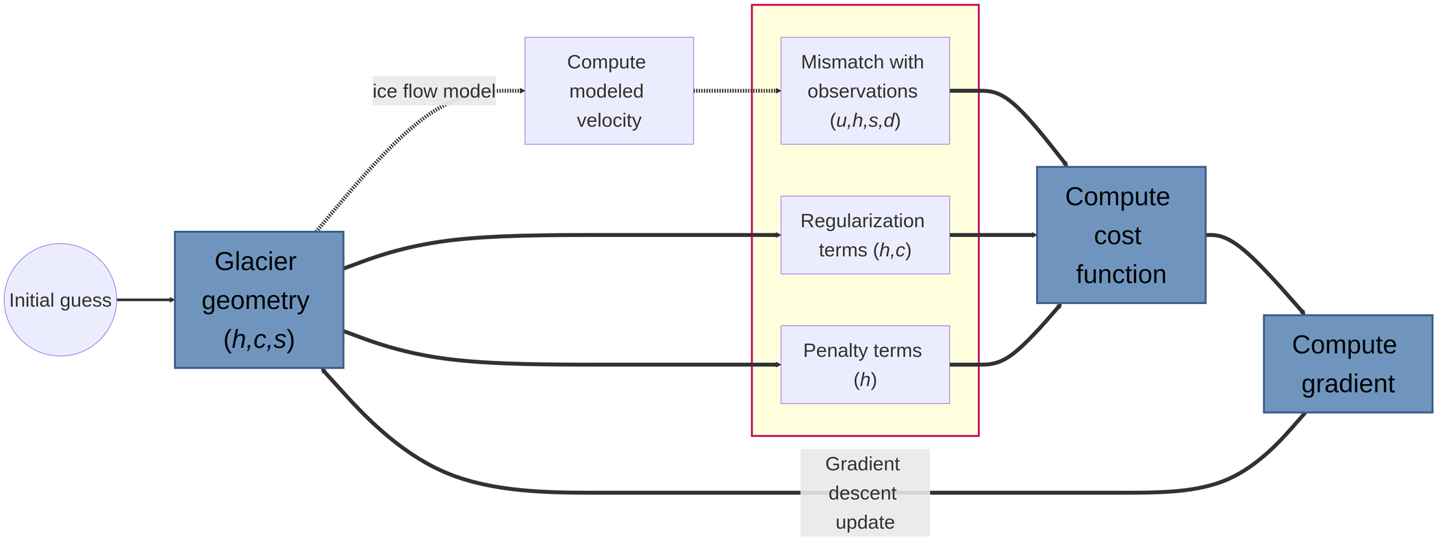


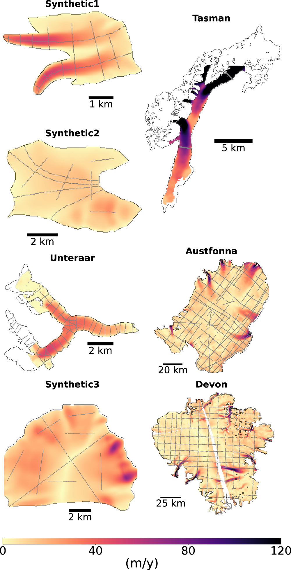


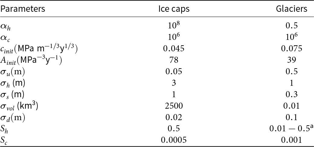


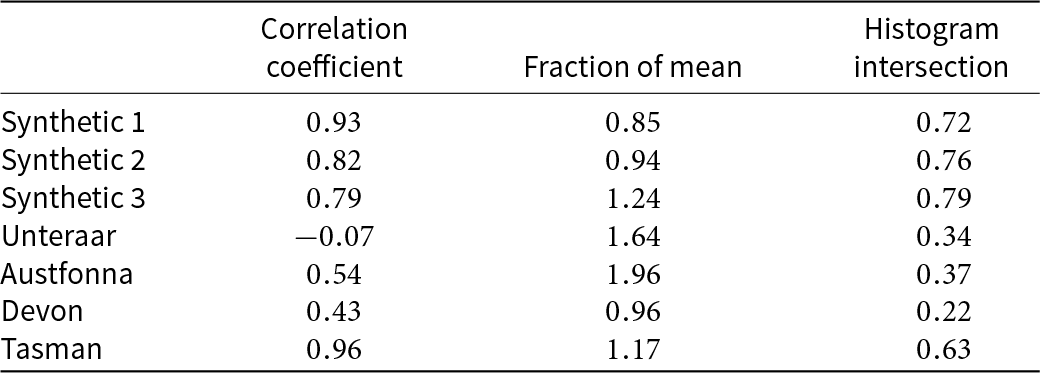


 Open access

