Introduction

The largest Antarctic ice shelves flow by forced horizontal extrusion through coastal embayments containing islands and sea-bed shoals. This extrusion is driven partly by seaward flow of outlet glaciers and ice streams entering the ice shelf and partly by the release of gravitational potential energy associated with local ice-shelf thinning (Reference WeertmanWeertman, 1957; Reference Swithinbank, Zumberge and HathertonSwithinbank and Zumberge, 1965; Reference BuddBudd, 1966). Basal melting can potentially modify this extrusion in three ways: (i) it can reduce the force that drives horizontal spreading; (ii) it can modify the total coastal friction resisting seaward flow; and (iii) it can cool the depth-averaged temperature and thus reduce the rate of ice-shelf deformation in response to a given stress.

Reference SandersonSanderson (1979) examined the first and second of these effects by calculating equilibrium ice-shelf thickness and velocity distributions for various idealized coastal embayments. His analysis demonstrated that spatially uniform melting increases the down-stream thickness slope and reduces the velocity and horizontal strain-rates. These changes result primarily from direct removal of ice-shelf mass which thereby reduces the gravitational driving stress. For embayments with straight but divergent coasts, uniform melting was found to shorten the length between the grounding line and the separation point where transverse spreading is no longer able to maintain contact between the ice shelf and coasts. By shortening this length, basal melting can potentially reduce the net coastal friction, or “back stress”, that maintains the dynamic stability of marine ice sheets (Reference ThomasThomas, 1979). Modification of this back stress may thus constitute a significant coupling between continental ice and the ocean.

Our investigation seeks to extend Reference Sanderson and DoakeSanderson’s (1979) results by evaluating the potential impact of basal melting on the present observed flow of the Ross Ice Shelf. Since we address the present ice-shelf thickness and size, our evaluation focuses on the effect of melting on the present depth-averaged temperature. Basal melting erodes the warmest part of the ice column nearest the ocean/ice interface and thereby lowers the depth-averaged temperature (Reference CraryCrary, 1961; Reference MacAyealMacAyeal, unpublished [b]). Strain-rates in ice under a fixed stress are strongly diminished by decreasing temperature (Reference HookeHooke, 1981) thus an ice shelf subject to basal melting will tend to stiffen. Although heat conduction within the ice column tends to counterbalance the effects of melting on the depth-averaged temperature, the thermal conductivity of ice is so low that conductive re-adjustment to a step-like basal melting change may take several hundred years (Reference MacAyealMacAyeal, unpublished [b]). During readjustment a typical ice column of a major Antarctic ice shelf can travel several hundred kilometers. It is therefore reasonable to expect reduced creep-rate “shadows” extending down-stream of localized sites of basal ablation. As an illustration of this concept, we present in Appendix A simple examples of ice-shelf response to basal melting that were generated using Reference Sanderson and DoakeSanderson’s (1979) methods.

To identify the thermal signature of basal melting in the Ross Ice Shelf flow, two methods are available: (i) conduct a comprehensive survey of temperature–depth profiles throughout the ice shelf with a horizontal resolution selected to detect the dominant spatial variability of basal melting zones, or (ii) use the observed relationship between thickness and deformation as a diagnostic indicator of thermal conditions. The first method is difficult because it requires ice drilling or electrical resistivity profiling (Reference Shabtaie and BentleyShabtaie and Bentley, 1979). Local surveys are possible (Reference Clough and HansenClough and Hansen, 1979; Reference Shabtaie and BentleyShabtaie and Bentley, 1979) but they are most useful for verification of precisely defined regions of basal melting. The second method is attempted in this study using observations made during the Ross Ice Shelf Glaciological and Geophysical Survey (RIGGS) and other field programs (Reference Zumberge and MellorZumberge, 1964; Bentley and others 1979; Reference Thomas, Thomas, MacAyeal, Eilers, Gaylord, Hayes and BentleyThomas and others, 1984).

In order to evaluate the relationship between observed thickness and deformation of a complex ice shelf potentially subject to spatially non-uniform melting, we must: (i) solve the momentum-balance and constitutive equations for the flow associated with non- uniform ice thickness and irregular boundaries, and (ii) solve the heat-transfer equation taking into account horizontal advection effects. In a previous paper (Reference Thomas and MacAyealThomas and MacAyeal, 1982), we reported results obtained from analytic formulae for ice-shelf spreading rates and a simple one-dimensional numerical treatment of heat transfer. The formulae are adequate to the extent that certain simplifying assumptions are satisfied by the complex thickness patterns and boundary conditions of the Ross Ice Shelf (see Reference Thomas and MacAyealThomas and MacAyeal, 1982). The one-dimensional heat-transfer analysis, however, is inadequate because it does not treat horizontal ice-column advection that may permit reduced creep-rate “shadows” to extend down-stream of restricted zones of basal melting.

In this study, we use the finite-element method to solve the momentum-balance, constitutive, and heat-transfer equations. This method provides a general solution for depth-independent flow in an ice shelf of any shape and provides a fully three-dimensional solution of the steadystate heat-transfer equation with horizontal advection terms. Here, we simulate ice-shelf flow and temperature distribution for two alternative basal melting scenarios and then compare these simulations with observations.

Despite the powerful and computationally expensive methods we use, we have not yet obtained acceptable agreement between simulated and observed flow patterns. This disagreement stems largely from inadequate boundary conditions required by numerical models such as ours. Nevertheless, we believe that our results provide several specific constraints on the nature of prevailing basal melting patterns, such as: (i) whether the pattern of basal melting required to maintain in “steady state” the observed ice-thickness distribution is compatible with observed creep rates; (ii) whether basal melting patterns implied by recent océanographie field work and theory are compatible with observed creep rates; and (iii) whether basal sea-ice layers derived from the above patterns are compatible with ice cores, radio echo-sounding, and electrical resistivity observations (Reference NealNeal, 1979; Reference Shabtaie and BentleyShabtaie and Bentley, 1979; Reference Zotikov, Zotikov, Zagorodnov, Raikovsky and RaykovskiyZotikov and others, 1980; Reference JezekJezek, 1984).

Governing Equations

The momentum and heat-balance equations used in this study are written:

(1)

and

(2)

where, x, y, z, t are horizontal (x and y) and vertical (z, positive upwards) coordinates (see Fig. 17) and time (t), and

Equation (1) describes the balance of forces within the ice (assumed to be crevasse-free), and can be solved for the ice velocity provided: (i) a constitutive relation is prescribed, and (ii) appropriate boundary conditions are specified. The constitutive relation used here is the “ice-flow law” adapted from that used by Reference Hooke, Hooke, Raymond, Hotchkiss and GustafsonHooke and others (1979) in a similar modeling study, and is written:

(3)

where, σ' is the deviatoric stress (Reference PatersonPaterson, 1969)

(4)

and

(5)

For simplicity, we assume that firn densification and elastic strains are uncoupled from the large-scale creep deformation. This assumption provides the incompressibility constraint

(6)

The symbols used above are

This constitutive relation is derived from laboratory measurements of the deformation of isotropic ice samples under applied loads (Reference GlenGlen, 1955; Hooke, 1981) and is consistent with field observations of unconfined ice-shelf flow (Reference ThomasThomas, 1973). The laboratory-derived values of B_O and Q used here represent soft ice conditions normally applicable at temperatures warmer than 260 K. Despite laboratory work indicating that ice colder than 260 K is stiffer with B ₀ and Q having values of 625 N m⁻² s^1/3 and 80 kJ mol⁻¹, respectively (Reference Barnes, Barnes, Tabor and WalkerBarnes and others, 1971), values representing softer, warmer ice are applied uniformly in this study. In view of the inadequate treatment of ice-shelf boundary conditions described below, a sensitivity analysis of B ₀ and Q would have been unproductive, so was not attempted. No attempt is made either to parameterize faults, crevasses, anomalous strain heating, and anisotropic fabric. The factor ρ(z)/ρ _i in Equation (5) represents our ad hoc representation of firn-layer strength. A more accurate treatment of firn-layer strength, perhaps using a Coulomb rheology (Reference Jaeger and CookJaeger and Cook, 1976), could potentially improve the model in regions of low ice thickness where firn comprises a major part of the ice column.

Fig. 1.

Observed thickness of the Ross Ice Shelf (Bentley and others, 1979). Coordinates indicated along the edges of this map are called “grid-coordinates” and are adopted here to be consistent with published maps of field data (e.g. fig. 1 of Bentley and others (1979)). In the grid-coordinate system, the North Pole is placed at the intersection of the Equator and the prime meridian. All directions, latitudes, and longitudes explicitly referred to in the text are taken with respect to the geographical coordinate system. All map projections presented here are polar stereographic and are referenced to the geographic South Pole.

The horizontal components of long-term and large-scale ice-shelf flow under consideration here are naturally independent of depth because thickness gradients, basal shear stresses, and variation of viscosity with depth are insufficient to induce significant vertical shear (Weertman, 1957; Sanderson and Doake, 1979). This property allows us to simplify our model by integrating Equation (1) over depth to eliminate one spatial dimension from the numerical domain. Equation (2) must be solved within a three-dimensional domain, however, because vertical and horizontal processes operate simultaneously. The numerical techniques used in this study are described in Appendix B.

Solution of Equation (1) through (6) provides a “snapshot” of the instantaneous flow and temperature. Time dependence of the flow is governed by the mass-balance equation (not shown), determining H(t) and the heat equation determining θ(t). In this study, the ice-thickness distribution is held fixed at its present observed state, shown in Figure 1. The time-derivative term in the heat equation is retained artificially, however, and is used as a computational technique for generating a temperature distribution in steady-state balance with a prescribed basal melting scenario and self-consistent with the temperature-dependent flow velocities. This technique of coupling ice-shelf dynamics and thermodynamics is referred to as “asynchronous coupling” and is discussed in detail under a separate heading.

Boundary Conditions

Velocity or stress must be prescribed on all surfaces bounding the ice shelf as boundary conditions for Equation (1). On the ice front and ice-shelf base, we specify hydrostatic sea-water pressure (assuming a constant sea-water density ρ _w of 1028.0 kg/m³ appropriate to Ross Sea conditions (Reference Jacobs, Jacobs, Gordon and ArdaiJacobs and others, 1979)) and zero shear stress. On the upper ice-shelf surface, we specify zero total stress (we disregard atmospheric effects). Velocity or stress conditions at the grounded-ice/floating-ice and the floating-ice/mountain-wall contacts are generally unknown because of insufficient field observation. Here we specify all such boundary conditions in terms of velocity. Along stagnant ice margins (edges of ice rises, edges of grounded ice where no outlet glacier or ice stream exists, mountain (Fig. 2) walls), we arbitrarily set the velocity to zero. For glaciers flowing through the Transantarctic Mountains and for West Antarctic ice streams (see Figure 2 and Reference HughesHughes (1975), Reference Giovinetto, Giovinetto, Robinson and SwithinbankGiovinetto and others (1966), and Reference SwithinbankSwithinbank (1963) for descriptions and locations of these geographic features), we specified velocities estimated from neighboring ice-shelf measurements. These velocities and associated ice-volume fluxes are compared with field observations in Table I.

Fig. 2.

Names of locations and features on the Ross Ice Shelf. Ice-stream and glacier influx are shown schematically.

Differences between the observed velocities and the specified input velocities result from finite grid resolution and our attempt to correctly represent within limits of error the observed ice-volume flux (defined as the integral of velocity over the cross-sectional area of the outlet glacier or ice stream). The finite limit of spatial resolution (10 km) inherent in our numerical grid necessitated some adjustment of the input velocity from that observed (assumed constant over the width of the glacier or ice stream) to attain the desired flux. In addition, we favored an increased value of the ice-volume flux (within the limits of observed error, if relevant) to account for other glaciers not explicitly modeled and for general ice-sheet drainage between ice streams.

For ice streams A through F, few field data are available to constrain our input velocities and fluxes. We thus extrapolated the desired input velocities from neighboring points on the ice shelf where velocities were observed during RIGGS (see Thomas and others (1984) for description of observations). We remark that agreement between the observed and simulated flow along the eastern grounding line could have been improved had we used higher ice-stream input velocities and fluxes. Such high velocities would have exceeded the upper boundary we believe to constrain plausible ice-stream velocities. In fact, our input velocities are well above those inferred from ice-thickness patterns by Reference RobinRobin (1975). We therefore suspect that specified ice-stream input velocities must presently be unrealistically high so as to overcome excessive restraining forces produced by the model elsewhere in the ice shelf.

Equation (2) describes the evolution of the temperature in response to both vertical and horizontal advection, and to vertical conduction. Horizontal conduction and viscous heat generation are disregarded in our model. The vertical variation of conductivity, heat capacity, and velocity in the firn layer are also disregarded because of insufficient vertical resolution which is 1/9 the local ice thickness. Boundary conditions required for Equation (2) are: (i) the surface temperature (θ_S ) determined from observed 10 m bore-hole temperatures Reference Thomas, Thomas, MacAyeal, Eilers, Gaylord, Hayes and Bentley(Thomas and others, 1984), (ii) the basal freezing temperature (θ_b) determined from the pressure-dependent freezing-point relation at an assumed salinity of 34.75‰ (Reference Fujino, Fujino, Lewis and PerkinsFujino and others, 1974), and (iii) the temperature–depth profile at all ice-stream inflow boundaries. For want of observations, condition (iii) is computed from a version of Equation (2) in which the horizontal advection terms have been truncated. This results in a version of condition (iii) that idealizes the ice streams and outlet glaciers as being charcteristically similar to ice shelves. To obtain w(z), we apply the incompressibitity constraint and adopt a stretched vertical coordinate system to account for snow accumulation denoted by Ȧ (m of ice/s) and basal accumulation denoted by Ḃ (m of ice/s) (see Appendix B). Values of Ȧ derived from RIGGS observations (see Thomas and others, 1984) were used as model input and are shown in Figure 3. For some of the experiments, Ḃ was specified; in others, Ḃ was constrained to balance the effects of snow accumulation and ice-shelf spreading. For computational purposes, we specify an analytic approximation to a steady-state temperature profile (Crary, 1961) as an initial condition. This condition is “forgotten”, however, because Equation (2) is integrated through time while artificially holding H(t) fixed until a “steady-state” temperature distribution is obtained.

Table I.Ice-Stream and Glacier Input Parameters

Fig. 3.

Observed snow-accumulation rate expressed in meters of ice equivalent per year Reference Thomas, Thomas, MacAyeal, Eilers, Gaylord, Hayes and Bentley(Thomas and others, 1984).

Asynchronous Coupling

The goal of our investigation is to determine the thermodynamic signal of basal melting in the present deformation rate of the Ross Ice Shelf. This presents a serious difficulty because the temperature distribution depends on past ice-shelf history; whereas, the deformation rate results from present instantaneous distributions of ice thickness and temperature. To calculate present ice-shelf temperature correctly, it is necessary to prescribe ice thickness and flow over the prior history of the ice shelf. This history is not sufficiently known to make such a calculation possible. We compromise by calculating instead the prior thermal evolution while artificially holding ice thickness fixed at its present value. We call this procedure asynchronous time marching (see Reference Manabe and BryanManabe and Bryan, 1969).

In brief, our procedure is; (i) step Equation (2) forward in time until θ converges to a stationary solution while holding H, Ȧ, θ_ḅ, and θ_S fixed at the present observed values, and holding Ḃ fixed at a prescribed value, and (ii) periodically update u to account for horizontal advection-rate changes caused by feedback between temperature and the flow-law parameter B. During this artificial time evolution, initial conditions are “forgotten”; and the temperature distribution and temperature-dependent ice velocities approach a self-consistent steady state. The temperature and effective viscosity are stepped forward through 3000 years of “evolution” with velocity updated every 50 years to account for the changing flow-law parameter. The prescribed basal melting rate is updated every 500 years, if it was specified using information derived from the simulated flow fields (see next section), We stress that this asynchronous time-marching scheme is artificial and is useful only to provide a self-consistent estimate of the present temperature and temperature-dependent advection patterns. This scheme represents an outgrowth of previous techniques used successfully to simulate observed bore-hole temperatures (Reference MacAyeal and ThomasMacAyeal and Thomas, 1979; Reference YoungYoung, 1981; Reference MacAyealMacAyeal, unpublished [b]).

In practice, we found that the above procedure would converge provided imposed basal freezing rates were not tied to simulated horizontal divergence rates in zones of high divergence down-stream of ice rises. In such cases, we found that positive feedback between warm temperatures associated with freezing and high flow divergence forced the temperature and flow to diverge from a reasonable solution. We did not continue these divergent simulations to see what alternative steady-state solutions would exist.

Zero Basal Ablation vs Maintenance of Steady State

We performed three simulations to evaluate the differences in ice-shelf flow between an imposed absence of basal melting and an imposed basal melting/freezing rate consistent with maintenance of steady-state ice thickness. In Run 1 we set Ḃ = 0. The velocity vectors and magnitude describing this simulation are shown in Figures 4 and 5. In Run 2, we unsuccessfully tried to impose a basal melting rate consistent with a steady-state ice thickness in its present configuration:

(8)

where is the observed snow-accumulation rate expressed in meters of ice per year shown in Figure 3 (Thomas and others, 1984). H is the observed ice thickness (Bentley and others, 1979) (Fig. 1), and u is the horizontal velocity calculated by the numerical model. A spatial smoothing operator, denoted by , was applied to the divergence term to eliminate irregular grid-point-to-grid-point “spikes” having the minimum spatial scale resolvable by our numerical model (10 km). This smoothing was accomplished by setting the value of ∇_H·(uH) at each interior grid point of our model domain equal to the average of its value at the eight closest interior grid-point neighbors (see Appendix B). Both Ḃ and u were updated periodically during the asynchronous time-marching procedure to insure compatability between 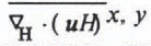and the changing effective viscosity.

Fig. 4.

The simulated velocity vectors of Run 1 are plotted at every other grid point. These velocities are assumed independent of depth.

Fig. 5.

The simulated isotachs of Run 1. These can be compared with the observed isotachs displayed in figure 1 of Reference MacAyeal and ThomasThomas and MacAyeal (1982).

Convergence was not achieved for Run 2 because of an unstable positive feedback between basal freezing and strong ice divergence 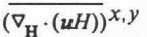in the lee of Crary and Steershead Ice Rises. To illustrate this point, Figure 6 presents a map of the simulated thickening tendency 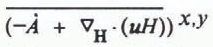associated with Run 1 (zero Ḃ). If the rule expressed by Equation (8) for specifying Ḃ is applied to the thickening tendencies shown in Figure 6, then substantial basal freezing is required in the central sections of the ice shelf and particularly down-stream of Crary and Steershead Ice Rises. Warming of the depth-averaged temperature associated with this freezing would tend to increase the ice-divergence rates, which in turn would require greater freezing rates and even warmer temperatures. We terminated our simulation of Run 2 once the ice-front velocities exceeded about 2000 m/year, which is about twice their observed value.

Fig. 6.

The ice-thickness growth rate (∂H/∂t) of Run 1 is contoured at intervals of 0.25 m/year. The zero-growth contour is eliminated but regions of ice thinning are indicated by shading.

Convergence failure in Run 2 resulted primarily from zones of high ice divergence occurring down-stream of the two major ice rises. These zones are generic parts of the typical ice-flow “signature” associated with ice rises in our numerical model. We postulated in a previous study that up-stream convergence combined with down-stream divergence comprises this “signature” and implies up-stream ice-rise migration along sea-bed ridges extending parallel to the flow lines (MacAyeal and Thomas, 1983). We further speculated that such migration could be organized into a quasi-periodic “wave train” of several ice rises situated along a sea-bed ridge, such as those ridges common to the Ross Sea (Reference Greischar and BentleyGreischar and Bentley, 1980; Reference Kirchner, Kirchner, Bentley and RobertsonMacAyeal and Thomas, 1982), Recent analysis of field data by Jezek (1984) lends some support to our speculation by indicating that the down-stream (north-western) edge of Crary Ice Rise has migrated up-stream over the last several hundred years.

Conditions immediately down-stream from an ice rise may be incompatible with steady state for two reasons: first, because of ice-rise migration; and secondly, because of ice-shelf fracture and cavitation. Consequently, we chose to abandon Run 2 and to run a third simulation in which imposed basal melting was sufficient to maintain steady state in all regions except for the zones of high divergence down-stream of ice rises. In these zones, basal freezing was limited to the value given by a balance between latent-heat release and upward heat flux through the ice shelf. We additionally imposed a high basal melting rate (5.0 m/year) within a 10 km strip along the ice front. This additional feature was imposed to test the proposition that diminished observed strain-rates along the ice front imply high local basal melting (Thomas and MacAyeal, 1982). The values of B imposed in Run 3 are

(9)

where k (2.24 W m⁻¹ K⁻¹) is the conductivity of ice at the freezing temperature (Weller and Schwerdtfeger, 1971) and L (3.35 × 10⁵ J/kg⁻¹) is the latent heat of fusion (Weast, 1968). Convergence of the asynchronous time-marching scheme was successful. Figure 7 shows the values of B that resulted from Equation (9) once the flow and temperature distributions converged. Figure 8 shows the velocity-magnitude difference between Runs 1 and 3.

Fig. 7.

The basal melting rate of Run 3 is contoured at intervals of 0.25 m/year (ice equivalent). The zero-melting contour is eliminated but regions of freezing are indicated by shading.

The comparison shown in Figure 8 indicates that the effect of basal melting is to reduce the simulated ice velocity up-stream of Crary Ice Rise by as much as 20% (see Fig. 5). This reduction results from the cooler depth-averaged temperature and the associated increased value_of the depth-averaged flow-law parameter (denoted by B ^Z ). The distributions of B ^Z for Runs 1 and 3 are shown in Figures 9 and 10, Respectively.

Fig. 8.

The velocity magnitude difference between Run 1 and Run 3 is contoured at intervals of 25.0 m/year.

Fig. 9.

The depth-averaged flow-law parameter (B^Z) of Run 1 is contoured at intervals of 10⁸ (N m⁻² s^1/3).

Fig. 10.

The depth-averaged flow-law parameter ( B ^Z ) of Run 3 is contoured at intervals of 10⁸ (N m⁻² s^1/3). Regions of basal melting in excess of 0.5 m/year are indicated by shading.

The plot of B ^Z for Run 3 shown in Figure 10 demonstrates the effect of horizontal advection. High values of B ^Z are not simply localized in the zones of basal melting shown in Figure 7 but extend for a limited distance down-stream. The shading in Figure 10 delimits the zones of melting greater than 0.5 m/a. Lobes of high B ^Z are found to extend down-stream of these regions, particularly in the vicinity of Crary Ice Rise.

Comparison with Observations

The difference between the velocities of Run 1 and the observed values (see Thomas and others, 1984) is shown in Figure 11 scaled by the observed velocity magnitude. Figure 12 shows observed and simulated horizontal strain-rates. In general, agreement is good, with simulated velocities within ±30% of observed values. The largest differences occur near the ice rises, and the results from Run 3 do not show any systematic improvement when compared with the observed values (Figs 8 and 11). Consequently, we cannot endorse either of the basal melting scenarios of Runs 1 or 3 as being “correct”. We have, however, demonstrated that within the limits of our modeling capability both scenarios are plausible. Moreover, the significant differences between results from Runs 1 and 3 indicate that basal melting conditions have a major effect on ice-shelf deformation.

Fig. 11.

The difference between the observed velocity and the simulated velocity of Run 1, divided by the magnitude of the observed velocity, is plotted to display model performance (observations are taken from Reference Thomas, Thomas, MacAyeal, Eilers, Gaylord, Hayes and BentleyThomas and others (1984)).

Fig. 12.

The observed horizontal strain-rates (right figure) are represented by cross-like patterns denoting the orientation, magnitude, and sign of the principal components. The simulated horizontal strain-rates of Run 1 (left figure) are shown for comparison at the same approximate locations as where the observations were taken.

Three basic patterns associated with Crary Ice Rise, Roosevelt Island, and Byrd Glacier are apparent in the differences between the calculated and observed velocities and strain-rates. Figure 11 indicates that simulated outflow of ice stream B passes more to the east of Crary Ice Rise than it should. This error may be attributable to smaller, less distinct ice-shelf grounding zones to the east and south-east that were not represented in the simulation. These ice rises, visually observed by Bindschadler (personal communication; see also Reference Thomas and BentleyThomas and Bentley, 1978) detected in radio echo-sounding data (Jezek, 1984; personal communication from S. Shabtaie) and evident in crevasse patterns (personal communication from A.P. Crary) may redirect the outflow of ice stream B to the west of Crary Ice Rise.

Simulated ice velocities both to the east and to the south-west of Roosevelt Island are lower than observed (Fig. 11); simulated shear resistance at the margins of their channels is too large. We attribute this excessive resistance to (i) sub-mesh-scale processes such as crevassing, shear heating, and preferred fabric development that are not parameterized, and (ii) inadequate resolution.

Model error in simulating the outflow of Byrd Glacier is again representative of excessive resistance. On examining the simulated stress patterns, we found that excessive restraint in this case is maintained by tensile stresses exceeding 10⁵ Pa (1 bar) that couple the stagnant ice on either side of the outflow to the mountain walls. Field studies (Reference HughesHughes, 1977; Reference BrecherBrecher, 1982) indicate that these marginal shear zones are ruptured and therefore are incapable of transmitting tensile stress.

Bore-hole observations of temperature are too few and too widely spaced to resolve the general patterns of melting and freezing implied by our simulations. Figure 13 shows the comparison between computed and observed temperature–depth profiles at the two locations, J9 and Little America V (LAV), where bore holes have completely penetrated the ice shelf (Crary, 1961; Clough and Hansen, 1979). We remark that some discrepancy in this comparison is inevitable because of (i) mismatch between the actual ice thickness and the ice thickness used by the model (interpolated from RIGGS data to a 10 km grid, (ii) mismatch between the actual surface temperature and the surface temperature used by the model, and (iii) (in the case of J9) the tendency for the simulated flow to pass farther to the east of Crary Ice Rise than the observed flow. Nevertheless, the mismatch between the simulated and observed J9 temperature profile implies that the melting zone of Run 3 located up-stream of Crary Ice Rise is incorrect. If a time-independent basal melting zone actually exists up-stream of Crary Ice Rise, the J9 data will then restrict it to regions not previously traversed by the J9 ice column.

Fig. 13.

The observed and simulated temperature–depth profiles at J9 and Little America V are plotted for comparison (Reference CraryCrary, 1961; Reference Clough and HansenClough and Hansen, 1979).

Observations of basal ice-layer composition indicate 6 m of basal sea ice at J9, and possibly thicker sea ice elsewhere (Neal, 1979; Zotikov and others, 1980; Jezek, 1984). Basal sea ice at J9 may seem inconsistent with the simulated basal melting pattern up-stream. Consideration of the heat fluxes that cause basal freezing, however, suggests that basal melting can actually amplify basal freezing at points down-stream. The factors to be considered are: (i) basal melting increases the vertical temperature gradient and upward heat flux in the basal ice layers (MacAyeal, unpublished [b]), (ii) increased upward heat flux does not diminish immediately when the ice column advects out of a basal melting area, and (iii) the increased upward heat-flux preconditions the ice column to strong basal freezing once it advects into regions where sensible heat is unavailable in the water column below. The enhancement of basal freezing by the thermal gradient steepening associated with basal melting must be considered in any interpretation of geophysical evidence for basal sea-ice accretions (MacAyeal and Thomas, 1979; Neal, 1979; Zotikov and others, 1980; Jezek, 1984). In the case of J9, where the sea-ice accretion and the temperature–depth profile are both known, there is little question as to the unlikelihood of strong basal melting up-stream. Observations of basal sea-ice accretions alone, however, cannot completely eliminate the possibility of basal melting in some regions sufficiently far up-stream.

Oceanographic Considerations

The simulated flow of Run 3 provides an approximate estimate of basal melting needed to maintain steady ice thickness (neglecting possible transient ice-rise effects). Here we examine oceanographic theory and field observations to test the plausibility of this estimate. Figure 7 presents B given by Run 3. The basic pattern suggests that there is a bi-modal melting regime: (i) melting in the remote parts of the cavity up-stream of Crary Ice Rise and Roosevelt Island, and (ii) melting in a strip along the ice front. Ice-shelf draft patterns imply that these two categories should produce melt-water masses observed at different levels of the Ross Sea water column.

Hydrographic and isotopic observations conducted by Reference Jacobs, Jacobs, Fairbanks, Horibe and JacobsJacobs and others (1985) confirm that ice-shelf melt water occurs at two distinct depths in the open Ross Sea. The deepest melt water is called deep ice-shelf water (DISW) and results from contact between the ice shelf and dense high-salinity shelf water (HSSW), formed by winter sea-ice production north of the ice front (Reference GillGill, 1973; Reference KillworthKillworth, 1974), Judging from its depth, DISW probably originates where the ice-shelf draft exceeds 400 m (indicated by shading in Figure 1). This draft requirement is satisfied by the regions of basal melting in Figure 7 up-stream of Crary Ice Rise and Roosevelt Island. The shallowest melt water is called shallow ice-shelf water (SISW) and is identified with basal melting along the ice-front areas in contact with a warm offshore water mass called the warm “core” (WMCO).

Possible DISW formation in the melting zone of Figure 7 up-stream of Crary Ice Rise is supported by the océanographie theory of tidal-front formation (Reference MacAyealMacAyeal, 1984, Reference MacAyeal and Jacobs1985[a]). Figure 14 displays the water-column thickness (depth) in the sub-ice-shelf cavity. The reduced water-column thickness in the region up-stream of Crary Ice Rise and along the Siple Coast promotes efficient vertical mixing as a result of tidally generated turbulence. This mixing, in turn, erodes density stratification and promotes contact between relatively warm, but dense, HSSW and the ice. Observations taken through the J9 bore hole approximately 100 km north-east of Crary Ice Rise show that stratification does persist in the regions where the water column is thicker than 100 m (Jacobs and others, 1979; Reference FosterFoster, 1983). This observed stratification suppresses contact between the ice and the warm HSSW, and permits weak basal freezing as evidenced by the J9 ice core (Zotikov and others, 1980). The two vertically well-mixed layers observed at J9 near the ice and the sea bed do, however, extend through about 80 m of the water column. These two mixed layers will thus likely merge to eliminate stratification where the water column is less than 80 m thick.

Fig. 14.

The observed water-column thickness (depth) of the Ross Sea and sub-ice-shelf cavity (Reference Greischar and BentleyGreischar and Bentley, 1980). The dotted line denotes the ice-front position.

Possible SISW formation in the ice-front melting zone of Figure 7 is also supported by the theory of tidal rectification (MacAyeal, 1985[b], unpublished [a]). Tidal rectification denotes the generation of time-independent circulation by periodic tidal currents passing across the depth discontinuity at the ice front (Reference ZimmermanZimmerman, 1981). A numerical simulation of tidal rectification in the Ross Sea indicates that oceanic heat advection into the cavity would be favored near Ross Island and near Roosevelt Island (MacAyeal, 1985[b]). Figure 15 displays the simulated oceanic advection patterns by showing the trajectories of imaginary passive tracers released along the ice front and near Steershead Ice Rise. Deepest penetration into the sub-ice-shelf cavity after 7.5 years of tracer advection occurs near Ross Island and north-west of Roosevelt Island. The 7.5 years time period corresponds roughly to the geochemic-ally derived sub-ice-shelf flushing time (Reference Michel, Michel, Linick and WilliamsMichel and others, 1979). The inability of trajectories to penetrate all regions of the sub-ice cavity indicates that tidal rectification alone is insufficient to ventilate the cavity at the observed rate. An estimate of the heat flux associated with this simulated ventilation, however, is sufficient to explain the basal melting along the ice front derived in Run 3.

Fig. 15.

Simulated tracer trajectories emanating from the ice front and from a position near Steershead Ice Rise are plotted to represent oceanic ventilation of the sub-ice-shelf cavity after 7.5 years of advection. These streak lines were generated by a numerical simulation of tidal current rectification (Reference MacAyeal and JacobsMacAyeal, 1985[b], Reference MacAyealunpublished [a]).

Conclusion

Our simulations have demonstrated that ice-shelf flow is thermodynamically coupled to basal ablation. This coupling was compared in two simulations of the present flow of the Ross Ice Shelf. In one simulation the basal melting rate was assumed zero everywhere, and in the other it was prescribed so that it would counterbalance the large-scale ice-thickening tendencies. The maximum flow difference between the two simulations was over 75 m/year in the region up-stream of Crary Ice Rise. Although this difference amounts to approximately 20% of the observed flow, it is not sufficient to explain discrepancies between the simulations and the observed flow, which are probably due to inadequate knowledge of the boundary conditions, sub-grid-scale softening of marginal ice, and to our over-simplified choice of laboratory-derived flow-law parameters. Once these conditions and effects are better understood, diagnostic determination of prevailing basal melting conditions from comparisons between observed and simulated large-scale flow patterns may be possible for all of the major Antarctic ice shelves.

Our analysis indicates that the spatial pattern of basal melting required to maintain present ice-shelf thickness in steady state (except for possible transient ice-rise migration) is plausible. We cannot confirm, however, whether the magnitude of melting required to maintain steady state is also plausible. To determine the magnitude, direct measurement and/or vertical profiles of ice-shelf temperatures are required. The spatial distribution of melting derived from our analysis is also found to be qualitatively compatible with oceanographic theory and observations that suggest a bi-modal circulation. We suspect that deep traces of ice-shelf melt water found in the open Ross Sea originate up-stream of Crary Ice Rise or Roosevelt Island where our model indicates ice-flow convergence, and that shallow traces originate near the ice front.