1 Introduction
The processes of the formation of sand dunes (Andreotti, Claudin & Douady Reference Andreotti, Claudin and Douady2002a ,Reference Andreotti, Claudin and Douady b ; Hersen, Douady & Andreotti Reference Hersen, Douady and Andreotti2002; Hersen et al. Reference Hersen, Andersen, Elbelrhiti, Andreotti, Claudin and Douady2004; Elbelrhiti, Claudin & Andreotti Reference Elbelrhiti, Claudin and Andreotti2005; Reffet et al. Reference Reffet, Du Pont, Hersen and Douady2010) and avalanches (Savage & Hutter Reference Savage and Hutter1991; Campbell, Cleary & Hopkins Reference Campbell, Cleary and Hopkins1995; Hutter et al. Reference Hutter, Koch, Pluüss and Savage1995) involve the surface flow of granular material on a fixed bed of the same material. Such surface flows are also prevalent in industrial systems such as rotary kilns and blast furnaces, as well as in heap storage of granular material (Perry & Green Reference Perry and Green1997). In these systems, the flowing granular material may deposit on the bed or erode the bed, depending on local conditions. The first theoretical studies of flows on erodible beds (Bouchaud et al. Reference Bouchaud, Cates, Prakash and Edwards1994; Boutreux, Raphaël & de Gennes Reference Boutreux, Raphaël and de Gennes1998) postulated the rate of deposition (volume per unit area per unit time) of particles on the bed to depend only on the local surface angle and to be of the form
 $$\begin{eqnarray}\unicode[STIX]{x1D6E4}=V(\unicode[STIX]{x1D6FD}_{n}-\unicode[STIX]{x1D6FD}^{\prime }),\end{eqnarray}$$
where
 $\unicode[STIX]{x1D6FD}^{\prime }$
is the surface angle and
 $\unicode[STIX]{x1D6FD}_{n}$
and
 $V$
are model parameters:
 $\unicode[STIX]{x1D6FD}_{n}$
is termed the neutral angle and
 $V$
is a characteristic velocity. The model, referred to as the BCRE model, implies that deposition of particles on the fixed bed (
 $\unicode[STIX]{x1D6E4}>0$
) occurs when the surface angle is smaller than the neutral angle (
 $\unicode[STIX]{x1D6FD}^{\prime }<\unicode[STIX]{x1D6FD}_{n}$
) and the bed is eroded (
 $\unicode[STIX]{x1D6E4}<0$
) when the surface angle is larger than the neutral angle (
 $\unicode[STIX]{x1D6FD}^{\prime }>\unicode[STIX]{x1D6FD}_{n}$
). Continuum models, based on depth-averaged mass and momentum balance equations and different assumptions for the closure terms, yield expressions for the deposition rate similar to (1.1) (Douady, Andreotti & Daerr Reference Douady, Andreotti and Daerr1999; Khakhar et al.
Reference Khakhar, Orpe, Andresen and Ottino2001).
Experimental studies of the flow on erodible beds have been carried out primarily in quasi-two-dimensional (quasi-2-D) systems (Grasselli & Herrmann Reference Grasselli and Herrmann1999; Lemieux & Durian Reference Lemieux and Durian2000; Khakhar et al.
Reference Khakhar, Orpe, Andresen and Ottino2001; Komatsu et al.
Reference Komatsu, Inagaki, Nakagawa and Nasuno2001; Taberlet et al.
Reference Taberlet, Richard, Valance, Losert, Pasini, Jenkins and Delannay2003; Midi Reference Midi2004; Jop, Forterre & Pouliquen Reference Jop, Forterre and Pouliquen2005, Reference Jop, Forterre and Pouliquen2006; Forterre & Pouliquen Reference Forterre and Pouliquen2008; de Ryck et al.
Reference de Ryck, Zhu, Wu, Yu and Zulli2010; Fan et al.
Reference Fan, Umbanhowar, Ottino and Lueptow2013; Martínez et al.
Reference Martínez, González-Lezcano, Batista-Leyva and Altshuler2016; Fan et al.
Reference Fan, Jacob, Freireich and Lueptow2017), in which the flow occurs between vertical plates, typically separated by a distance of 10–20 particle diameters. We briefly summarize the results relevant for the present study. Several studies of flow on an erodible bed in quasi-2-D systems have shown that the velocity profile is approximately linear over most of the flowing layer depth (Komatsu et al.
Reference Komatsu, Inagaki, Nakagawa and Nasuno2001; Taberlet et al.
Reference Taberlet, Richard, Valance, Losert, Pasini, Jenkins and Delannay2003; Midi Reference Midi2004; Jop et al.
Reference Jop, Forterre and Pouliquen2005; Orpe & Khakhar Reference Orpe and Khakhar2007; Forterre & Pouliquen Reference Forterre and Pouliquen2008), and is an assumption used in several continuum models (Douady et al.
Reference Douady, Andreotti and Daerr1999; Khakhar et al.
Reference Khakhar, Orpe, Andresen and Ottino2001). However, this is an approximation since the transition between the flowing layer and the fixed bed is not sharp and the velocity decays exponentially, resulting in slow creeping motion of the particles deep in the bed (Komatsu et al.
Reference Komatsu, Inagaki, Nakagawa and Nasuno2001; Martínez et al.
Reference Martínez, González-Lezcano, Batista-Leyva and Altshuler2016). Khakhar et al. (Reference Khakhar, Orpe, Andresen and Ottino2001) carried out a detailed experimental test of (1.1) in a quasi-two-dimensional rectangular system with pouring at one closed edge, to form a heap. The neutral angle was experimentally measured for steady continuous flow on a heap in an open system (far edge open) and the rate of deposition and the surface angle in a closed system (far edge closed) in which the heap grew uniformly with time (Khakhar et al.
Reference Khakhar, Orpe, Andresen and Ottino2001). The experimental results showed (1.1) to be valid, with
 $V$
obtained from the model of Khakhar et al. (Reference Khakhar, Orpe, Andresen and Ottino2001). Equation (1.1) was also found to be valid for the flow in a quasi-two-dimensional rotating cylinder, partly filled with grains (Orpe & Khakhar Reference Orpe and Khakhar2001). The neutral angle is found to increase with thickness of the flowing layer (Khakhar et al.
Reference Khakhar, Orpe, Andresen and Ottino2001; Taberlet et al.
Reference Taberlet, Richard, Valance, Losert, Pasini, Jenkins and Delannay2003; Jop et al.
Reference Jop, Forterre and Pouliquen2005). Taberlet et al. (Reference Taberlet, Richard, Valance, Losert, Pasini, Jenkins and Delannay2003) showed that this increase is due to side wall friction. The neutral angle is larger than the angle of repose (surface angle in the limit of no flow) in all cases. Side wall friction has a significant effect on the flow, even for the case of wider gaps between the side walls (Jop et al.
Reference Jop, Forterre and Pouliquen2005, Reference Jop, Forterre and Pouliquen2006).
There have been only a few studies on the formation of three-dimensional heaps. Altshuler et al. (Reference Altshuler, Ramos, Martínez, Batista-Leyva, Rivera and Bassler2003) and Altshuler et al. (Reference Altshuler, Toussaint, Martínez, Sotolongo-Costa, Schmittbuhl and Måløy2008) studied the dynamics of formation of conical sand heaps by pouring sand on a circular disc of finite diameter. Initially, the heap grew by avalanches distributed azimuthally. However, when the height of the heap exceeded a certain value, a narrow stream of sand flowing from the apex to the base of the heap started rotating around it (shown schematically later in the paper), which left a spiral layer of sand deposited on the free surface in each revolution, leading to the growth of the heap. The spiral mode of heap growth was sensitive to the size of the heap; it was not observed for very small and large heaps. The angular velocity (
 $\unicode[STIX]{x1D714}$
) of the revolving stream was found to depend on time (
 $t$
) as
 $\unicode[STIX]{x1D714}\sim t^{-2/3}$
(Altshuler et al.
Reference Altshuler, Ramos, Martínez, Batista-Leyva, Rivera and Bassler2003; Kong et al.
Reference Kong, Hu, Wu and Wu2006; Altshuler et al.
Reference Altshuler, Toussaint, Martínez, Sotolongo-Costa, Schmittbuhl and Måløy2008). The studies pertaining to the sand dunes (Andreotti et al.
Reference Andreotti, Claudin and Douady2002a
,Reference Andreotti, Claudin and Douady
b
; Hersen et al.
Reference Hersen, Douady and Andreotti2002, Reference Hersen, Andersen, Elbelrhiti, Andreotti, Claudin and Douady2004; Elbelrhiti et al.
Reference Elbelrhiti, Claudin and Andreotti2005; Reffet et al.
Reference Reffet, Du Pont, Hersen and Douady2010) are not directly relevant for the present work, since the granular flow is wind driven in these cases.
A schematic representation of the steady surface flow on a part of the surface of an asymmetric heap. The coordinate system is shown along with the direction of gravity (
 $\boldsymbol{g}$
). The disc diameters are shown as dashed lines. The pouring point (demarcated by a black circle) is adjusted at some distance from the disc centre, to yield a surface flow in the
 $x$
direction.

We consider heap formation on a circular disc when the pouring point is displaced from the centre of the disc, with the objective of characterizing flows on an erodible bed in the absence of bounding side walls, which are known to significantly affect the flow. In the growth phase, the heap is axisymmetric, and we characterize the dynamics of growth. A steady flow is established when the base of the heap reaches the edge of the disc and particles begin to flow over the edge of the disc, as shown schematically in figure 1. The geometry is a unique example of a granular flow on an erodible bed without any bounding side walls. It has direct relevance for natural systems, such as avalanches and sand dunes, but has not previously been studied in detail. The heap geometry at steady state is characterized by means of contour lines at different heights and by angles of repose. The streamwise and transverse velocity profiles are measured at the surface using high-speed photography and image analysis. The flowing layer thickness profile is also measured at a few points on the mid-line of the flow. A depth-averaged model is presented, and the predictions of the model for the layer thickness are compared to the experimental results. The organization of the paper is as follows: experimental details are given in § 2, experimental results are reported in § 3, followed by conclusions in § 4.
2 Experimental details
2.1 System
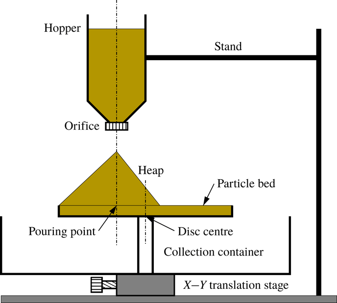
A schematic view of the experimental set-up is shown in figure 2. A conical hopper of capacity 1900 cm
 $^{3}$
with a circular orifice, suspended above a circular disc of diameter 30 cm with the help of two rods attached to the base, is used to pour the material. The orifice at the throat of the hopper is interchangeable, and orifices of different diameters are used to yield different mass flow rates. The disc has a lip of height 16 mm at its edge, which enables the formation of a shallow packed bed of the working material, providing a rough base. The disc is fixed above a cylindrical container to collect the particles which spill over the edge of the disc. The disc can be moved horizontally relative to the orifice using two screws. We perform most experiments using nearly monodisperse spherical glass beads of diameter
 $d=1.3\pm 0.05~\text{mm}$
and a few sets using glass beads of diameter
 $d=0.7\pm 0.06~\text{mm}$
. The glass beads are coloured with permanent red marker ink to yield a uniform glossy surface, which helps detection during image analysis.
A schematic representation of the experimental set-up with different parts labelled.

2.2 Experimental method
Initially, we calibrated the orifices by measuring the weight of beads collected over a fixed duration of time to obtain the mass flow rate for each orifice. The mass flow rates from the orifices were found to be constant over time, and the mass flow rates obtained for the different orifices are:
 ${\dot{m}}=7.5$
, 14.7 and
 $21.4~\text{g}~\text{s}^{-1}$
. The hopper is filled with material, and the circular disc is adjusted so that the pouring point is 7 cm away from the centre of the disc (figure 1). The resulting heap is big enough and the flowing layer is sufficiently thick for studying the steady surface flow on top of it for the chosen value of off-centre distance. In some experiments, the disc is adjusted so that the pouring point is at the centre of the disc. A bed of glass beads of height equal to the height of the lip is prepared on the disc. The vertical distance between orifice tip and the top surface of the granular bed, i.e. the maximum falling height is 16 cm for all the experiments with off-centre pouring and 10 cm for the experiments with pouring at the centre of the disc. A high-speed camera (Phantom V12.1 with a Zoom-NIKKOR 35–70 mm lens) is used to capture the heap formation process.
In the study of the dynamics of heap formation, when the heap is axisymmetric, the axis of the camera is aligned horizontally at the level of the circular disc. A halogen display lamp is focused on the disc from the front. The process is continuously recorded from the beginning until the heap front reaches the circumference of the disc, and particles begin to overflow. The movies are captured at 24 frames per second and a resolution of
 $1280\times 800$
pixels with an exposure of 3 ms. The movies are converted into images for further analysis. A software package (ImageJ) is used to measure the height of the heap and the angle of repose in each image. The experiment is repeated five times for each flow rate, and the reported results are averaged over five sets. The experiments are also performed in two different seasons when the relative humidity is very different: during the monsoon season, when the relative humidity is approximately 90 %, and in the winter season, when it is approximately 60 %.
In steady surface flow experiments, a rough base is prepared on the circular disc as in the previous case. The flow is then initiated, and a heap grows until one edge reaches the periphery of the disc and a steady flow is established (figure 1). The pouring is then stopped, and the high-speed camera is focused with its axis perpendicular to the free surface of the heap. The area in the vicinity of the apex is excluded to avoid the bouncing particles. The halogen lamp is also focused perpendicular to the heap surface to illuminate the flowing particles down the heap surface. Since the free surface of the heap is curved, the scale factor changes with position on the direction transverse to the flow. To obtain the correct scale factors at different positions, the static heap is carefully wrapped with a mm graph paper keeping the camera setting unchanged, and a still photograph is captured. ImageJ is then used to calculate scale factors at different positions. The material is then removed from the disc, and the pouring is again initiated from the beginning to form the heap. Video recording of the particle motion is initiated when the particles begin to flow over the edge of the disc, at 500 frames per second and a resolution of
 $1280\times 800$
pixels, and continued for 30 s. The movies are then converted into a series of images. The images corresponding to initial 20 s are not considered (to eliminate any transient effects), and the remaining images are processed to obtain the velocities of the particles, as described in appendix A. The experiment is repeated five times for each flow rate.
We use the following intrusive method to measure the flowing layer thickness, which is a variant of the method of Jop et al. (Reference Jop, Forterre and Pouliquen2005). A metal needle of diameter 1.4 mm is blackened using the flame of a candle and is carefully inserted into the flowing layer, normal to the free surface, at a given position along the mid-line of the flowing layer. The part of the needle in contact with the flowing layer gets coated with flakes of the red paint used to colour the particles, as shown in figure 3. Thresholding of the image is done to highlight the coated region. The needle is removed after an interval of 50 s, and the length of the coated region is measured using a mm scale. This is taken to be an estimate of the flowing layer thickness.
A coated needle with soot on its surface (a) before and (b) after insertion into the flowing layer. (c) A magnified view of the coated region in (b). Thresholding of the image is done to highlight the coated region.

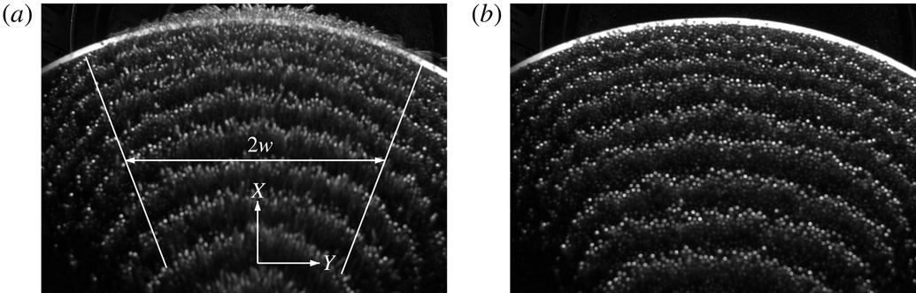
We determine the shape of the heap during and after the steady surface flow by projecting equally spaced horizontal lines using a digital projector from the front of the heap. The projection of the lines on the heap free surface yields contours (figure 4). The contours are captured from the top, keeping the axis of a digital camera (Nikon D3100) vertical.
Typical contour images of an asymmetric heap (a) during and (b) after the surface flow of 1.3 mm beads at the mass flow rate of
 $14.7~\text{g}~\text{s}^{-1}$
for off-centred pouring, captured from above. The flow occurs in the
 $x$
direction in the marked region of variable width
 $2w$
in (a).

3 Results and discussion
3.1 Evolution of axisymmetric heaps
The pouring of particles on the disc results in the formation of a conical heap which grows with time, as shown in figure 5 for a typical case. The heap remains axisymmetric during its growth. The pouring of particles at the centre of the disc results in a heap which grows to the full size of the disc. The experiments with the smaller beads (0.7 mm) and pouring at the disc centre, yield two different modes of surface flow depending on the humidity. At low humidity, the surface flow comprises local avalanches down the heap surface in random directions. Under humid conditions, the surface flow comprises periodic avalanches (rotating), which rotate around the heap with an angular speed
 $\unicode[STIX]{x1D714}$
, as shown schematically in figure 6. A rotating stream with a clear front (figure 6
d), as reported previously by Altshuler et al. (Reference Altshuler, Ramos, Martínez, Batista-Leyva, Rivera and Bassler2003) for sand heaps, was not seen in our experiments, most likely because the particles used in our experiments are significantly larger. The heap remains geometrically similar in the two cases. The particles are dry and there are no liquid bridges formed. The humidity only reduces the charge on the particles, which results in a more compact stream of particles falling from the hopper. The humidity has no effect on the flow on the heap.
Different stages of an axisymmetric heap (front view) formed by pouring glass beads of 1.3 mm on the circular disc at the off-centre position at the mass flow rate of
 $14.7~\text{g}~\text{s}^{-1}$
. The images are at different times (a)
 $t=10$
s, (b)
 $t=20$
s, (c)
 $t=30$
s and (d)
 $t=40$
s, the end. The angle of repose, denoted by
 $\unicode[STIX]{x1D6FD}$
, is shown in (b). The dashed line in (b) shows the tilt at the apex.

Observation indicates that the mode of the flow during the formation of the conical heap depends sensitively on the shape of the heap at its apex. A perfectly horizontal surface at the apex would yield a uniform surface flow, i.e. axially symmetric. However, such a configuration is unstable, and a small tilt causes a flow in that direction. This results in a build-up of material in that direction and thus changes the direction of the tilt azimuthally. The tilt is clearly apparent in figure 5(b), where the plane of the apex is marked with a dashed line. In the two modes observed, the change of direction of the tilt of the surface at the apex azimuthally with time is random in the case of random avalanches and periodic in the case of periodic avalanches. In the periodic flow mode, the particles are deposited in the wake of the previous avalanche. In contrast, in the random growth mode, the deposition of particles occurs at random (low lying) azimuthal locations on the free surface. The periodic avalanche mode is observed only after the heap grows to a finite size and occurs only for the bigger heaps (pouring at the disc centre) for the smaller particles (0.7 mm diameter).
A schematic representation of the periodic avalanche (shown in dark yellow shade) in (a–c). Time increases from (a) to (c). A spiral stream of particles (shown in dark yellow shade), as observed by Altshuler et al. (Reference Altshuler, Ramos, Martínez, Batista-Leyva, Rivera and Bassler2003), rotates in the direction of arrow in (d).

Variation of the (a–c) heap height (
 $h$
) and (d–f) angle of repose (
 $\unicode[STIX]{x1D6FD}$
) with time (
 $t$
) for different mass flow rates in different cases. (a,d) Periodic mode for the pouring of 0.7 mm beads at the disc centre; (b,e) random mode for the pouring of 0.7 mm beads at the disc centre; (c,f) random mode for the off-centred pouring of 1.3 mm beads. Dashed lines are predictions of (3.1) in (a,b) and (3.2) in (c).

Figure 7 shows the variation of the height (
 $h$
) of the heap and the corresponding heap surface angle (
 $\unicode[STIX]{x1D6FD}$
) with time (
 $t$
) for the different cases studied. Figure 7(a,b) show a comparison of heap growth by the periodic avalanche and random avalanche modes for 0.7 mm particles poured at the centre of the disc, while figure 7(c) shows heap growth by the random avalanche mode for the 1.3 mm particles, with the pouring point off centre. Data for three different mass flow rates (
 ${\dot{m}}$
) are shown for each case. The increase in height of the heap with time is nearly identical for the periodic avalanche (figure 7
a) and random avalanche (figure 7
b) growth modes, the differences arising because of differences in the angles of repose for the two modes, which are small (figure 7
d,e). The final height for the case of 1.3 mm beads (figure 7
c) is significantly smaller due to off-centre pouring. The angle of repose (
 $\unicode[STIX]{x1D6FD}$
) decreases with time during the initial period and then remains nearly constant in each case (figure 7
d–f). The final angle is independent of mass flow rate in each case. A volume balance, assuming the heap to be a right circular cone and the angle of repose to be constant, yields the variation of the heap height with time as
 $$\begin{eqnarray}h=\unicode[STIX]{x1D6FC}t^{1/3},\end{eqnarray}$$
where
 $\unicode[STIX]{x1D6FC}=(3{\dot{m}}\tan ^{2}\unicode[STIX]{x1D6FD}/\unicode[STIX]{x03C0}\unicode[STIX]{x1D70C}_{b})^{1/3}$
and
 $\unicode[STIX]{x1D70C}_{b}$
is the bulk density, measured to be
 $\unicode[STIX]{x1D70C}_{b}=1.5~\text{g}~\text{cm}^{3}$
. The dashed lines in figure 7(a,b) show the predictions of (3.1) using the measured values of the bulk density and angle of repose, which match the experimental data quite well. Equation (3.1) does not work well for the smaller heap (figure 7
c), since the error in omitting the flattening of the apex of the cone becomes significant. Taking this into account, a volume balance yields
 $$\begin{eqnarray}h=(h_{0}^{3}+\unicode[STIX]{x1D6FC}^{3}t)^{1/3}-h_{0},\end{eqnarray}$$
where
 $h_{0}$
is the height of the missing apex of the cone. The predictions of (3.2) (dashed lines, figure 7
c) closely match the experimental data, with
 $h_{0}$
found from (3.2) by using a single data point (
 $h,t$
) measured near the end of the experiment. The above results show that the scaling,
 $h\propto t^{1/3}$
, reported by Altshuler et al. (Reference Altshuler, Ramos, Martínez, Batista-Leyva, Rivera and Bassler2003), is valid for larger heaps.
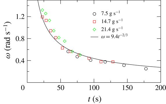
Variation of the angular velocity (
 $\unicode[STIX]{x1D714}$
) of the periodic avalanche of particles of
 $d=0.7~\text{mm}$
with time (
 $t$
) for the pouring at the disc centre at different mass flow rates.

Figure 8 shows the variation of the angular velocity (
 $\unicode[STIX]{x1D714}$
) of the avalanches with time for three different mass flow rates, in the periodic avalanche mode. The data are given for times after the rotation starts. The angular velocity is nearly independent of mass flow rate and decreases with time. The scaling arguments of Altshuler et al. (Reference Altshuler, Ramos, Martínez, Batista-Leyva, Rivera and Bassler2003) can be extended to the case of periodic avalanches, as follows. For the heap shape to remain constant, a deposit of uniform thickness,
 $\unicode[STIX]{x1D6FF}_{s}$
, is formed in each revolution. A volume balance for the deposit in one revolution yields
 $$\begin{eqnarray}2\unicode[STIX]{x03C0}{\dot{m}}/(\unicode[STIX]{x1D714}\unicode[STIX]{x1D70C}_{b})=\unicode[STIX]{x03C0}\tan \unicode[STIX]{x1D6FD}((r+\unicode[STIX]{x1D6FF}_{s})^{3}-r^{3})/3,\end{eqnarray}$$
where
 $r$
is the radius at the base of the heap and the right-hand side of the equation is the increase in volume of the conical heap in one revolution. Retaining only terms of
 $O(\unicode[STIX]{x1D6FF}_{s})$
and simplifying, we get
 $$\begin{eqnarray}\unicode[STIX]{x1D714}=2{\dot{m}}/(\unicode[STIX]{x1D70C}_{b}r^{2}\unicode[STIX]{x1D6FF}_{s}\tan \unicode[STIX]{x1D6FD}).\end{eqnarray}$$
Taking
 $r=h/\tan \unicode[STIX]{x1D6FD}$
and using (3.1) we finally obtain
 $$\begin{eqnarray}\unicode[STIX]{x1D714}=Ct^{-2/3},\end{eqnarray}$$
where
 $C=2[\unicode[STIX]{x03C0}^{2}{\dot{m}}/(9\unicode[STIX]{x1D70C}_{b}\tan \unicode[STIX]{x1D6FD})]^{1/3}/\unicode[STIX]{x1D6FF}_{s}$
. The solid line in figure 8 is a least squares fit of (3.5) to the combined data for the three mass flow rates for
 $t>40$
s, with a fitted value
 $C=9.4$
, and shows good agreement with experimental data. A constant value of
 $C$
implies that the thickness of the deposit increases with mass flow rate as
 $\unicode[STIX]{x1D6FF}_{s}\propto {\dot{m}}^{1/3}$
, which is reasonable based on dimensional analysis. Analysing the experimental results in terms of (1.1) is difficult, since the flow is intermittent and the geometry is complex.
Side view of the asymmetric heap with the surface flow of 1.3 mm beads atop for the mass flow rate of
 $14.7~\text{g}~\text{s}^{-1}$
. The surface flow occurs in the
 $x$
direction. The angles in the flow direction are denoted by
 $\unicode[STIX]{x1D6FD}_{m1}$
,
 $\unicode[STIX]{x1D6FD}_{m2}$
and
 $\unicode[STIX]{x1D6FD}_{m3}$
and that in the opposite direction is denoted by
 $\unicode[STIX]{x1D6FD}$
.

The static and dynamic angles of repose for different mass flow rates.

3.2 Steady surface flow on asymmetric heaps
We consider steady flow on a heap surface when the pouring point is off centre. The heap is asymmetric in this case, as shown in figure 9. The surface angles, measured in the plane of symmetry (
 $\unicode[STIX]{x1D6FD}$
,
 $\unicode[STIX]{x1D6FD}_{m1}$
,
 $\unicode[STIX]{x1D6FD}_{m2}$
,
 $\unicode[STIX]{x1D6FD}_{m3}$
, figure 9), are given in table 1 for the different mass flow rates. The apex of the heap is slightly tilted in the direction of flow and makes an angle of
 $\unicode[STIX]{x1D6FD}_{m1}\approx 10^{\circ }$
with the horizontal. The free surface angle on the side with the flow is nearly constant in middle section of the heap (
 $\unicode[STIX]{x1D6FD}_{m2}$
) and increases near the base of the heap (
 $\unicode[STIX]{x1D6FD}_{m3}$
) due to end effects. The angles are nearly independent of mass flow rate. At steady state, the shape of the heap is constant, which implies that surface flow occurs on the fixed bed without deposition or erosion. In the context of (1.1),
 $\unicode[STIX]{x1D6E4}=0$
at steady state, so that the surface angle at all points on the flowing layer is approximately equal to the neutral angle (
 $\unicode[STIX]{x1D6FD}_{n}$
). Rather than considering surface angles, the basal interface angle is physically more relevant for defining the neutral angle, since this angle determines the angle of incipient failure of the fixed bed. An estimate of the neutral angle based on the basal interface angle, for present geometry, in which the layer thickness reduces due to spreading of the flow, is given below. The angle in the middle region (
 $\unicode[STIX]{x1D6FD}_{m2}$
) corresponds to the equilibrium neutral angle, since end effects are negligible. The results indicate that
 $\unicode[STIX]{x1D6FD}_{m2}$
is nearly constant for a near-threefold increase in the mass flow rate. This is at variance with the results of quasi-two-dimensional heaps (Khakhar et al.
Reference Khakhar, Orpe, Andresen and Ottino2001; Taberlet et al.
Reference Taberlet, Richard, Valance, Losert, Pasini, Jenkins and Delannay2003; Jop et al.
Reference Jop, Forterre and Pouliquen2005), in which a significant increase of the surface angle with mass flow rate is seen. The results indicate that, in the absence of side wall friction, the neutral angle is nearly independent of the mass flow rate. Further, the neutral angle (
 $\unicode[STIX]{x1D6FD}_{m2}$
) is significantly smaller than the angle of repose (
 $\unicode[STIX]{x1D6FD}$
), in all cases (table 1). This is in marked contrast to the results for quasi-two-dimensional systems in which the neutral angle is always larger than the angle of repose. This difference is due to the presence of side wall friction in the quasi-two-dimensional systems, which results in a significant increase in the neutral angle with flow rate and the higher angles are frozen in place when the flow stops.
The same contour curves within the marked area as in figure 4 after averaging for different mass flow rates (a) during and (b) after surface flow. The dashed lines are fitted arcs to the data.

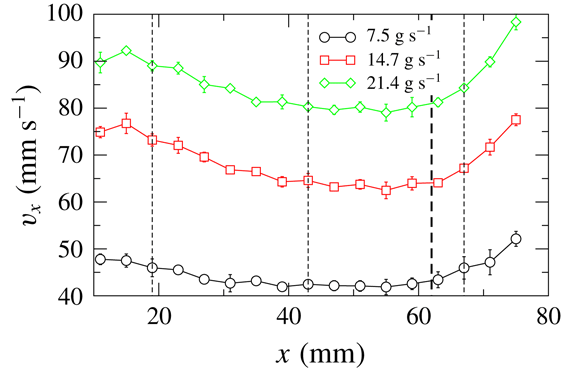
Variation of the streamwise surface velocity (
 $v_{x}$
) at the mid-line of the free heap surface (
 $y=0$
) with the streamwise distance (
 $x$
) from the apex for different mass flow rates. The thin dashed lines indicate the streamwise positions at which the velocity profiles in figures 12 and 14 are plotted. The thick dashed line demarcates the region where the angle increases from
 $\unicode[STIX]{x1D6FD}_{m2}$
to
 $\unicode[STIX]{x1D6FD}_{m3}$
.
The streamwise (
 $v_{x}$
) (symbols, a–c) and transverse (
 $v_{y}$
) (symbols, d–f) surface velocities as functions of the transverse distance (
 $y$
) from the mid-line of the free heap surface for different mass flow rates at different streamwise positions: (a,d)
 $x=19.0~\text{mm}$
, (b,e)
 $x=43.0~\text{mm}$
and (c,f)
 $x=67.0~\text{mm}$
. The dashed lines are fits of the functions as stated in the text.

Variation of half-width (
 $w$
) of the flow region with the streamwise distance (
 $x$
) from the apex for different mass flow rates. The dashed lines are the same as in figure 11.

Figure 10 shows the measured contours of the heap at different heights during flow (figure 10
a) and after the flow has stopped (figure 10
b). The contours during flow (figure 10
a) are nearly the same for the different flow rates in concurrence with the above results showing that the surface angles are nearly independent of the mass flow rates (table 1). The contours after flow for all the mass flow rates also overlap well (figure 10
b), as expected since the inclination angle of the heap (angle of repose,
 $\unicode[STIX]{x1D6FD}$
) is the same in all cases. The contours are approximated as arcs of circles, and the dashed lines in figure 10 correspond to the fitted curves. Since all the fitted arcs have the same centre, the distance between two contours is the same, indicating that the neutral angle is the same at all transverse positions on the flowing layer (figure 10
a).
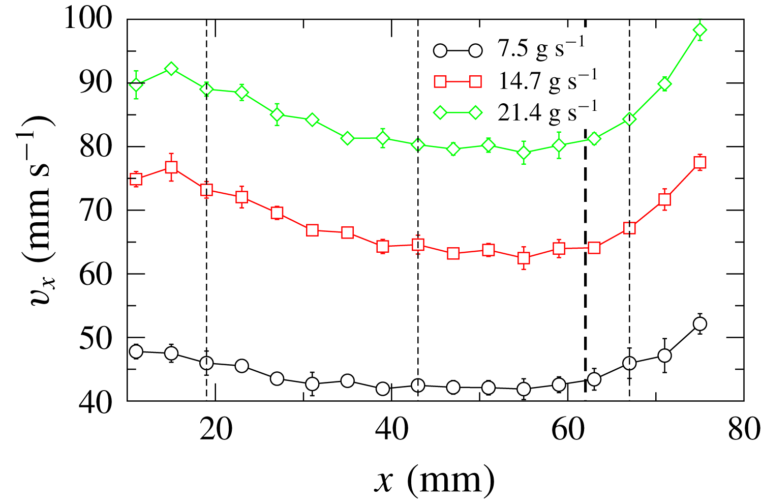
Figure 11 shows the variation of the streamwise mean surface velocity (
 $v_{x}$
) measured at the mid-line (
 $y=0$
) of the free heap surface with the streamwise distance (
 $x$
) from the apex. The velocity near the apex decreases with increasing distance, remains nearly constant over a small region and then increases. The surface velocity decreases with distance due to the reduction in the layer thickness as the flow spreads in the transverse direction. The increase is due to the higher surface angle near the base of the heap (
 $\unicode[STIX]{x1D6FD}_{m3}$
, table 1) and the thick dashed line in figure 11 shows the transition point between the middle region (surface angle
 $\unicode[STIX]{x1D6FD}_{m2}$
) and the edge region (surface angle
 $\unicode[STIX]{x1D6FD}_{m3}$
). The velocity increases with increasing mass flow rate.
The variation of the streamwise (
 $v_{x}$
) and the transverse (
 $v_{y}$
) surface velocities with transverse distance (
 $y$
), at three different streamwise positions (
 $x$
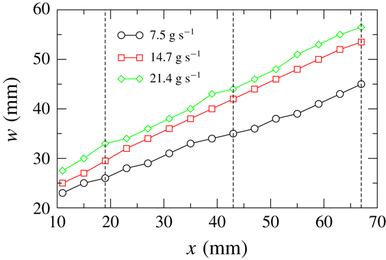
, marked by dashed lines in figure 11), is shown in figure 12 for the different mass flow rates. The streamwise velocity and the absolute transverse velocity profiles are symmetric about the mid-line. The streamwise velocity is maximum at the mid-line and the maximum/minimum transverse velocity occurs at a distance from the mid-line. The profiles are characteristic of a diverging flow. The transverse velocity is significantly smaller than the streamwise velocity, with the magnitude of the maximum transverse velocity being 5–10 % of the maximum streamwise velocity in all the cases. The variation of the half-width (
 $w$
) of the flow region with the streamwise distance (
 $x$
) is shown in figure 13. The half-width is taken to be the transverse distance from the mid-line to the point where the velocity is 4 % of the maximum velocity, i.e.
 $v_{x}(x,w)=0.04v_{x}(x,0)$
:
 $w$
shows a near-linear increase with increasing
 $x$
and increases with increasing mass flow rate.
The experimental velocity profiles were fitted with the following empirical equations
 $$\begin{eqnarray}\displaystyle & \displaystyle v_{x}=A\exp \left[-\frac{y^{2}}{2a^{2}}\right], & \displaystyle\end{eqnarray}$$
 $$\begin{eqnarray}\displaystyle & \displaystyle v_{y}=B\left(\frac{y}{b}\right)\exp \left[-\frac{y^{2}}{2b^{2}}\right], & \displaystyle\end{eqnarray}$$
where
 $A$
,
 $a$
,
 $B$
and
 $b$
are fitting constants. From the above equations we obtain the maximum streamwise velocity to be
 $v_{x}(x,0)=A$
and the maximum transverse velocity to be
 $v_{y}(x,b)=B\exp (-1/2)$
. The dashed lines in figure 12 show the fitted curves, and the values of the fitted constants are given in table 2. The proposed equations describe the experimental velocity profiles quite well. The experimental values of the maximum velocities (
 $v_{x}^{max}$
,
 $v_{y}^{max}$
) and
 $w$
are also given in table 2. The fitted values,
 $A$
,
 $B/\sqrt{e}$
, match the corresponding measured maximum velocities reasonably well and the parameters
 $a$
,
 $b$
are proportional to
 $w$
. The fitting shown above indicates that the velocity profiles are similar for the different flow rates and streamwise positions. This is considered next.
The measured values of the surface velocities and half-width of the flow region and the fitted constants for the velocity profiles for different mass flow rates.

When the streamwise (
 $v_{x}$
) and transverse velocities (
 $v_{y}$
) are scaled with their maximum values and the transverse distance (
 $y$
) with the half-width of the flow region (
 $w$
), the scaled profiles for different mass flow rates overlap well with each other, as shown in figure 14 for
 $v_{x}$
at one streamwise position. The scaled profiles for all three streamwise positions are nearly the same (not shown). The scaling again shows that the velocity profiles for different mass flow rates (
 ${\dot{m}}$
) and for different streamwise positions (
 $x$
) are similar. We now compare the scaled streamwise surface velocity profiles with those obtained in the flow over a erodible base in an inclined channel (Jop et al.
Reference Jop, Forterre and Pouliquen2005) qualitatively. The scaled velocity profiles for different flow rates (flow rate per unit width of the channel) for a given width of the channel (
 $2w$
) do not collapse, on the contrary. However, the deviation between the profiles is not much for a sixfold increase of the flow rate, except near the side walls (
 $y/w=-1,1$
). Hence, one can observe by comparing our data and the data of Jop et al. (Reference Jop, Forterre and Pouliquen2005) that the streamwise velocity profile becomes increasingly less uniform with increasing the width of the channel for a given flow rate – the velocity profile is nearly flat for low values of width and is Gaussian for an infinitely wide channel (no side walls).
The scaled streamwise surface velocities (
 $v_{x}/v_{x}^{max}$
) as functions the scaled transverse distance (
 $y/w$
) for different mass flow rates at
 $x=43.0~\text{mm}$
. The lines show the data in the study of Jop et al. (Reference Jop, Forterre and Pouliquen2005) for different cases.

We estimate the flowing layer thickness from the measured surface velocity distribution assuming that the mean velocity varies linearly over the flowing layer depth and the shear rate (
 $\dot{\unicode[STIX]{x1D6FE}}$
) is nearly constant in the transverse (
 $y$
) direction. The local volumetric flow rate (
 $Q$
) at any
 $x$
is determined as
 $$\begin{eqnarray}Q=\int _{-w}^{w}\int _{0}^{\unicode[STIX]{x1D6FF}(x,y)}V_{x}(x,y,z)\,\text{d}z\,\text{d}y,\end{eqnarray}$$
where
 $V(x,y,z)$
is the velocity field and
 $\unicode[STIX]{x1D6FF}(x,y)$
is the layer thickness. Putting
 $V_{x}(x,y,z)=v_{x}(x,y)(1-z/\unicode[STIX]{x1D6FF})$
in (3.8) and integrating with respect to
 $z$
, we obtain
 $$\begin{eqnarray}Q=\frac{1}{2\dot{\unicode[STIX]{x1D6FE}}(x)}\int _{-w}^{w}v_{x}^{2}(x,y)\,\text{d}y,\end{eqnarray}$$
where the shear rate is
 $$\begin{eqnarray}\dot{\unicode[STIX]{x1D6FE}}(x)=\frac{v_{x}(x,y)}{\unicode[STIX]{x1D6FF}(x,y)},\end{eqnarray}$$
assuming
 $\text{d}v_{x}/\text{d}z\gg \text{d}v_{x}/\text{d}y$
. Finally we get the flowing layer thickness as
 $$\begin{eqnarray}\unicode[STIX]{x1D6FF}(x,y)=\frac{2{\dot{m}}v_{x}(x,y)}{\displaystyle \unicode[STIX]{x1D70C}_{b}\int _{-w}^{w}v_{x}^{2}(x,y)\,\text{d}y},\end{eqnarray}$$
using the relation
 ${\dot{m}}$
=
 $\unicode[STIX]{x1D70C}_{b}$
 $Q$
.
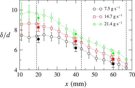
The layer thickness profile at the mid-line (
 $\unicode[STIX]{x1D6FF}(x,0)$
), computed from (3.11) using experimental values of the surface velocity (
 $v_{x}(x,y)$
) and carrying out the integration numerically, is shown in figure 15. The layer thickness decreases monotonically with increasing distance and increases with increasing mass flow rate. The values of the layer thickness (open symbols) computed from the model closely match the values directly measured from the experiments (filled symbols), validating the assumptions of the model (figure 15). The layer thickness values are smaller than those obtained in quasi-two-dimensional systems (Khakhar et al.
Reference Khakhar, Orpe, Andresen and Ottino2001) but appear to be reasonable: 4–10 particle diameters. Figure 16 shows the variation of the shear rate with the streamwise distance for different mass flow rates. The shear rate is nearly constant in the upper region of the heap and then increases with increasing distance and also increases with increasing mass flow rate. The shear rates are lower than the shear rates in quasi-two-dimensional systems, but of the same order of magnitude.
Variation of the normalized layer thickness (
 $\unicode[STIX]{x1D6FF}/d(y=0)$
) at the mid-line with the streamwise distance (
 $x$
) from the apex in different cases. Open symbols: theoretical values; filled symbols: experimentally measured values. The dashed lines are the same as in figure 11.

Variation of the shear rate (
 $\dot{\unicode[STIX]{x1D6FE}}$
) with the streamwise distance (
 $x$
) from the apex for different mass flow rates. The dashed lines are the same as in figure 11.

Since the layer thickness decreases with distance due to spreading of the flow, the surface angle is larger than the angle of the interface between the flowing layer and the fixed bed. Considering this, the neutral angle based on the inclination of the basal interface is given by
 $\unicode[STIX]{x1D6FD}_{n}=\unicode[STIX]{x1D6FD}_{m2}+\text{d}\unicode[STIX]{x1D6FF}/\text{d}x$
. We obtain
 $\text{d}\unicode[STIX]{x1D6FF}/\text{d}x$
by fitting straight lines to the experimental data in figure 15 and the values of the neutral angle for the three different flow rates are given in table 3. The angles are 4–
 $5^{\circ }$
smaller than the surface angle (
 $\unicode[STIX]{x1D6FD}_{m2}$
) and are independent of the mass flow rate.
The measured values of the equilibrium neutral angle (
 $\unicode[STIX]{x1D6FD}_{n}$
) taking into account the decreasing layer thickness, for different mass flow rates (
 ${\dot{m}}$
).

4 Conclusions
We report on an experimental study of the surface flow of glass beads on a heap, formed on a circular disc by pouring at a point from a hopper. A shallow fixed bed of the same material on the disc provides a rough base. In the first part of the work, we studied the dynamics of formation of the heap, which remained axisymmetric during its growth. The heap was found to grow by avalanches on different parts of the heap surface rather than by a continuous flow. Two modes of growth were observed: avalanches at random azimuthal positions on the heap surface and avalanches rotating in the azimuthal direction with a mean angular velocity. The latter was found to be prevalent in the case of smaller beads, larger heaps and when the humidity was high. The revolving rivers found by Altshuler et al. (Reference Altshuler, Toussaint, Martínez, Sotolongo-Costa, Schmittbuhl and Måløy2008) were not seen in our experiments. Experimental measurements indicated that the surface angle (angle of repose,
 $\unicode[STIX]{x1D6FD}$
) decreased slightly at the start of the growth and then remained constant. Using this result, volume balances yielded
 $h\propto t^{1/3}$
and
 $\unicode[STIX]{x1D714}\propto t^{-2/3}$
. The predictions of these equations were in good agreement with experimental measurements.
In the second part of the work we studied the steady surface flow on the heap, when the pouring point was off centre relative to the circular disc. The heap was asymmetric in this case and the heap geometry was characterized by means of surface angles in the mid-plane of heap and by surface contours. In the context of the BCRE-type models (Bouchaud et al.
Reference Bouchaud, Cates, Prakash and Edwards1994; Boutreux et al.
Reference Boutreux, Raphaël and de Gennes1998; Douady et al.
Reference Douady, Andreotti and Daerr1999) the surface angle at steady state corresponds approximately to the neutral angle, since there is no deposition or erosion of the heap. The neutral angle, based on the inclination of the basal interface, was found to be
 $\unicode[STIX]{x1D6FD}_{n}\approx 16^{\circ }$
, independent of mass flow rate (over a threefold increase) and approximately 10
 $^{\circ }$
less than the angle of repose (
 $\unicode[STIX]{x1D6FD}\approx 26^{\circ }$
). These results are in sharp contrast to measurement in quasi-two-dimensional systems, which show a significant increase in the neutral angle with mass flow rate (layer thickness) and in which the neutral angle is always larger than the angle of repose. Both these differences are due to the side wall friction in quasi-two-dimensional systems. The surface contours were well approximated by arcs of circles with the same centre, indicating that the neutral angle is nearly independent of the azimuthal angle.
Surface velocity measurements showed that the velocities decreased with distance from the apex due to decrease in the flowing layer thickness as the width of the flowing region increased with distance. The velocities increased with distance near the base due to end effects. The magnitude of the transverse velocity was approximately 10 % of the streamwise velocity in all cases. Gaussian functions were found to describe the measured velocity profiles with reasonable accuracy, indicating that the velocity profiles, at different positions and at different mass flow rates, were similar. This was also seen from the overlap of the scaled velocity profiles.
A simple model, in which the velocity profile in the layer was assumed to be linear and the velocity gradient was assumed to be independent of the transverse distance, was used together with the measured velocity profiles to predict the flowing layer thickness. The predicted layer thickness was found to decrease, nearly linearly, with distance from the apex, and to increase with mass flow rate. The predicted layer thickness was in good agreement with the measured values.
The results presented in this work provide a detailed characterization of surface granular flow on an erodible bed, in the absence of side wall effects. The measurements of contours, velocity and layer thickness profiles provide data useful for the development and validation of models. The finding that the neutral angle is smaller than the angle of repose is significant from a practical view point. The results imply that when flow starts on a static heap, a considerable amount of material is eroded from the heap to achieve the neutral angle, which is smaller than the angle of repose. Such eroded material would add to the volume of the surface flow and has implications for the modelling of natural (e.g. avalanches) and industrial systems.
Acknowledgements
The authors acknowledge the financial support of the Science and Engineering Research Board, India through grant SR/S2/JCB-34/2010.
Appendix A. Image analysis
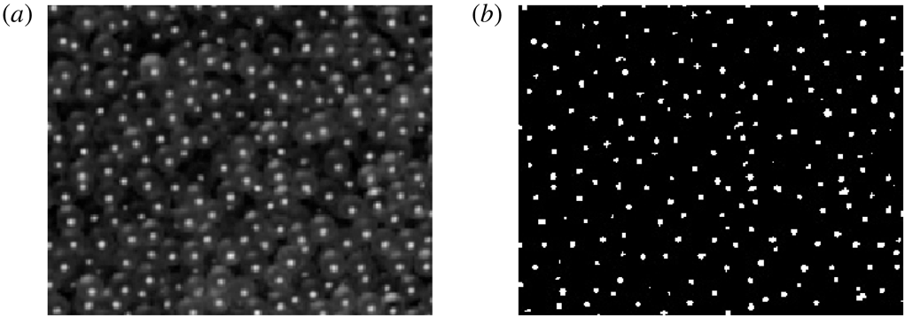
The image analysis technique followed here is the same as the one used by Mandal & Khakhar (Reference Mandal and Khakhar2017). Since the exteriors of the particles are smooth and reflective, a large bright spot appears on each of them due to the primary reflection of light. A code, written in C, is used to detect the particles based on the grey-scale intensity of the pixels of bright spots. The pixels with intensity greater than the threshold limit are considered, and they form clusters as shown in figure 17. Again a threshold limit on the cluster size is chosen, and the clusters with sizes exceeding the threshold limit are considered as particles. We obtain the positions of the particles as the centroids of the clusters in pixels in each image from this analysis. The positions in pixels are converted into mm by multiplying by the local scale factor. The trajectories of the particles are obtained following the same technique as used by Mandal & Khakhar (Reference Mandal and Khakhar2017). Instantaneous velocities of a particle,
 $c_{xi}$
and
 $c_{yi}$
, in the
 $x$
and
 $y$
directions are computed by dividing its displacements over two consecutive images by the time lapse between the images (
 $2\times 10^{-3}~\text{s}$
). The area of each image is then divided into rectangular bins of size
 $1\times 1~\text{mm}^{2}$
to calculate average properties. The mean surface velocities,
 $v_{x}$
and
 $v_{y}$
, in
 $x$
and
 $y$
directions in a bin are computed as
 $$\begin{eqnarray}\displaystyle & \displaystyle v_{x}=\frac{1}{N}\mathop{\sum }_{i=1}^{N}c_{xi}, & \displaystyle\end{eqnarray}$$
 $$\begin{eqnarray}\displaystyle & \displaystyle v_{y}=\frac{1}{N}\mathop{\sum }_{i=1}^{N}c_{yi}, & \displaystyle\end{eqnarray}$$
where
 $N$
is the number of particles in the bin over all the images analysed.
(a) A typical image showing the bright spots on the glass beads. (b) The image after the detection of clusters.