1 Introduction
The dynamics of a droplet on an inclined plane driven by strong, vertical, sinusoidal oscillations has received much attention since the behaviour of this system was first studied experimentally by Brunet, Eggers & Deegan (Reference Brunet, Eggers and Deegan2007, Reference Brunet, Eggers and Deegan2009). Not only is the dynamics surprising (under the right circumstances, the droplet can climb uphill), but the flow is unsteady, nonlinear and, as we shall see, mainly controlled by the dynamics of the three-phase contact line at the boundary between liquid, air and the solid plane beneath the droplet. The unsteady dynamics of contact lines, particularly in the presence of contact angle hysteresis, remains poorly understood, and the experimental data of Brunet et al. (Reference Brunet, Eggers and Deegan2007, Reference Brunet, Eggers and Deegan2009), subsequently extended by Sartori et al. (Reference Sartori, Quagliati, Varagnola, Pierno, Mistura, Magaletti and Casciola2015) to a wider range of fluids, provide a test bed for theories of unsteady contact line motion, which is important in, for example, coating processes (Weinstein & Ruschak Reference Weinstein and Ruschak2004), inkjet printing (Derby Reference Derby2010) and digital microfluidics (Fair Reference Fair2007).
The usual approach to modelling unsteady flows with contact lines (see e.g. Hocking Reference Hocking1987; Billingham Reference Billingham2002) is to assume that the contact line velocity is a single-valued function of the apparent contact angle, which can either be deduced from more fundamental fluid mechanical considerations (e.g. Marsh, Garoff & Dussan V. Reference Marsh, Garoff and Dussan V.1993; Eggers & Stone Reference Eggers and Stone2004) or measured experimentally in a steady flow (e.g. Dussan V. Reference Dussan V.1979; Tanner Reference Tanner1979). Although we choose to use this approach in our initial analysis, the assumption that an unsteady flow is slow enough that the moving contact lines are quasi-steady is a strong one. There has been some theoretical progress on the effect of local flows on unsteady contact lines, particularly inertial effects (e.g. Cox Reference Cox1998; Sui & Spelt Reference Sui and Spelt2013), but experimental results are often hard to explain theoretically (e.g. Ting & Perlin Reference Ting and Perlin1995; Jiang, Perlin & Schultz Reference Jiang, Perlin and Schultz2004; and, of course, Brunet et al. Reference Brunet, Eggers and Deegan2007, Reference Brunet, Eggers and Deegan2009).
There have been several attempts to model and understand the experimental results of Brunet et al. (Reference Brunet, Eggers and Deegan2007, Reference Brunet, Eggers and Deegan2009), using a wide range of assumptions and approximations. John & Thiele (Reference John and Thiele2010) used the thin-film equation to model a viscous-dominated droplet with small contact angles, and found that a ratcheting mechanism, which acts through changes in the shape of the droplet, can cause it to climb. Benilov (Reference Benilov2010) studied a two-dimensional, quasi-static droplet (inertia and viscous stresses negligible compared to surface tension forces). His main result was that the droplet can be made to climb uphill if the acceleration of the plate is a combination of deep, narrow troughs and low, wide peaks, which was demonstrated analytically for small contact angles and numerically for the general case. However, the acceleration applied to the plate by Brunet et al. (Reference Brunet, Eggers and Deegan2007) was sinusoidal. Benilov (Reference Benilov2011) extended this approach to a three-dimensional droplet with small contact angles, which he found could climb uphill under the influence of a sinusoidal oscillation. In Benilov & Cummins (Reference Benilov and Cummins2013), this model was studied for arbitrary contact angles, and it was found that, as the static contact angle increases, the droplet begins to climb uphill at lower forcing amplitudes. However, when the magnitude of the contact angles reaches a critical size, dependent on the contact line law, the frequencies at which the droplet can climb are bounded above. In all of these models, no contact angle hysteresis was included. Bradshaw & Billingham (Reference Bradshaw and Billingham2016) extended the model of Benilov (Reference Benilov2011) to large-amplitude oscillations, which allowed them to examine the effect of contact angle hysteresis. They found that under some circumstances hysteresis can cause the droplet to climb faster, and also that the footprint of the droplet is qualitatively similar to that observed in experiments if the hysteresis interval is large enough.
In Benilov & Billingham (Reference Benilov and Billingham2011), the effect of fluid inertia, which it is hard to argue is negligible in the experiments, was included by using the two-dimensional inviscid shallow-water equations along with a variety of contact line laws, including hysteresis. It was found that, in this limit, the motion of the droplet under the action of small-amplitude forcing in the absence of hysteresis is due to the interaction between an odd (swaying) and an even (spreading) mode. The dynamics for larger-amplitude forcing also exhibits a combination of swaying and spreading motions. When hysteresis is present, it was found that the frequency at which the droplet climbs uphill fastest shifts towards the resonant frequency of the droplet with pinned contact lines, and that the greatest rise velocity (with rise velocity,
 $V_{r}$
, defined to be the velocity of the midpoint of the base of the droplet averaged over one period of the motion) increases in the presence of moderate hysteresis, a phenomenon that we will examine in more detail below. Both Borcia, Borcia & Bestehorn (Reference Borcia, Borcia and Bestehorn2014) and Sartori et al. (Reference Sartori, Quagliati, Varagnola, Pierno, Mistura, Magaletti and Casciola2015) used a two-dimensional phase field method to include the effect of viscous stresses, solving the full Navier–Stokes equations, with the motion of the contact lines controlled by the fluid–wall interaction model. Their results were qualitatively similar to those of Benilov & Billingham (Reference Benilov and Billingham2011). This numerical method does not give much control over the model for the contact line dynamics, and cannot simulate the effect of contact angle hysteresis.
In this paper, we will extend the analysis of Benilov & Billingham (Reference Benilov and Billingham2011), which assumed that the two contact angles of a two-dimensional droplet are small, to arbitrary contact angles. We retain the assumption that the flow is inviscid and irrotational. In § 2 we further discuss the assumptions that we have made and derive the governing equations for the flow. In § 3 we study the case of small-amplitude forcing and show that the rise velocity of the droplet is controlled by the weakly nonlinear interaction of odd and even linear modes of oscillation, consistent with the results of Benilov & Billingham (Reference Benilov and Billingham2011) for the case of small contact angles. In § 4 we outline our numerical solution method for the fully nonlinear free boundary problem, and discuss how the parameters affect the behaviour of the droplet. We also study a simple model for the motion of the contact line that includes a finite lag, and leads to contact line behaviour closer to that observed in experiments.
2 Governing equations
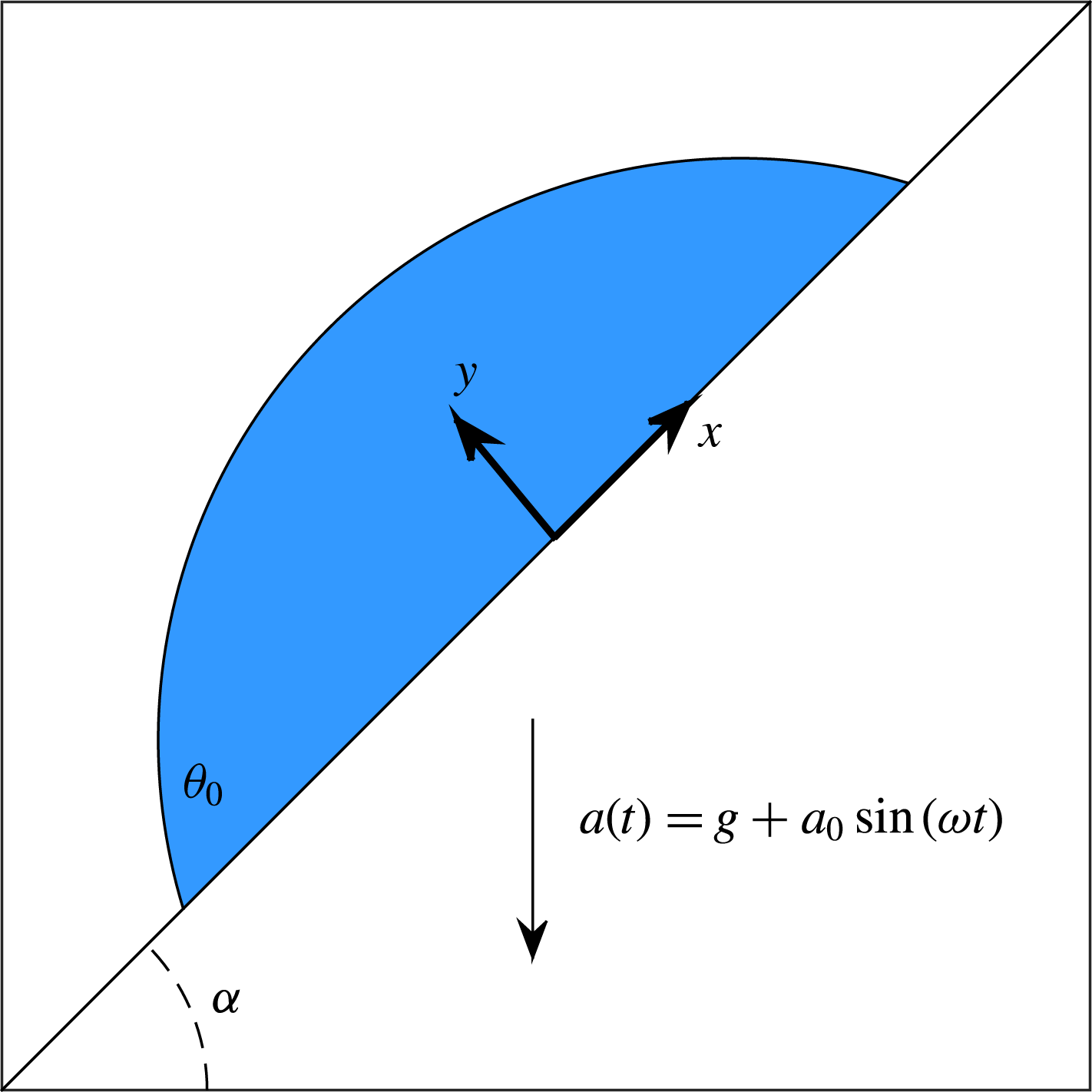
As discussed in § 1, our starting point will be the model for an inviscid, irrotational flow described in Benilov & Billingham (Reference Benilov and Billingham2011), but we will not make the small-contact-angle/shallow-water approximation. The Cartesian
 $(x,y)$
coordinate system is shown in figure 1. The inviscid fluid in the droplet has constant density
 $\unicode[STIX]{x1D70C}$
and its interface with the surrounding air has surface tension coefficient
 $\unicode[STIX]{x1D70E}$
. The fluid lies on a substrate inclined at angle
 $\unicode[STIX]{x1D6FC}$
to the horizontal that is oscillating vertically and sinusoidally with amplitude
 $a_{0}$
and frequency
 $\unicode[STIX]{x1D714}$
. The frame of reference is fixed in the substrate, so that the applied acceleration appears as a body force in the governing equations. In terms of a velocity potential,
 $\unicode[STIX]{x1D719}(x,y,t)$
, the boundary value problem that we must solve is
 $$\begin{eqnarray}\unicode[STIX]{x1D6FB}^{2}\unicode[STIX]{x1D719}=0,\end{eqnarray}$$
in the domain
 ${\mathcal{D}}(t)$
occupied by the fluid, with free boundary
 $\boldsymbol{x}\equiv (x,y)=\boldsymbol{X}(s,t)\equiv (X(s,t),Y(s,t))$
, where
 $s$
is arclength measured along the free surface, with
 $s=0$
at the contact line with smaller
 $x$
and
 $s=L(t)$
, the total arclength, at the other contact line. The dynamic boundary condition is
 $$\begin{eqnarray}{\displaystyle \frac{\unicode[STIX]{x2202}\unicode[STIX]{x1D719}}{\unicode[STIX]{x2202}t}}+{\displaystyle \frac{1}{2}}|\unicode[STIX]{x1D735}\unicode[STIX]{x1D719}|^{2}-{\displaystyle \frac{\unicode[STIX]{x1D70E}\unicode[STIX]{x1D705}}{\unicode[STIX]{x1D70C}}}+a(t)(X\sin \unicode[STIX]{x1D6FC}+Y\cos \unicode[STIX]{x1D6FC})=0\quad \text{on }\boldsymbol{x}=\boldsymbol{X}(s,t),\end{eqnarray}$$
where
 $\unicode[STIX]{x1D705}$
is the curvature of the free surface and
 $a(t)=g+a_{0}\sin \unicode[STIX]{x1D714}t$
is the effective body force due to gravity and the oscillation of the substrate. The kinematic boundary condition is
 $$\begin{eqnarray}\boldsymbol{n}\boldsymbol{\cdot }{\displaystyle \frac{\text{d}\boldsymbol{X}}{\text{d}t}}={\displaystyle \frac{\unicode[STIX]{x2202}\unicode[STIX]{x1D719}}{\unicode[STIX]{x2202}n}}\quad \text{on }\boldsymbol{x}=\boldsymbol{X}(s,t),\end{eqnarray}$$
where
 $\boldsymbol{n}$
is the outward unit normal. The impermeability of the substrate gives the boundary condition
 $$\begin{eqnarray}{\displaystyle \frac{\unicode[STIX]{x2202}\unicode[STIX]{x1D719}}{\unicode[STIX]{x2202}y}}=0\quad \text{on }y=0\text{ for }x_{-}(t)\leqslant x\leqslant x_{+}(t).\end{eqnarray}$$
The two contact lines are at
 $x=x_{\pm }(t)$
. We will assume that the velocity of a contact line with contact angle
 $\unicode[STIX]{x1D703}$
measured through the fluid is a single-valued function
 $v(\unicode[STIX]{x1D703})$
, as discussed above, where
 $$\begin{eqnarray}\left.\begin{array}{@{}cl@{}}v(\unicode[STIX]{x1D703})<0 & \text{for }\unicode[STIX]{x1D703}<\unicode[STIX]{x1D703}_{R},\\ v(\unicode[STIX]{x1D703})=0 & \text{for }\unicode[STIX]{x1D703}_{A}\geqslant \unicode[STIX]{x1D703}\geqslant \unicode[STIX]{x1D703}_{R},\\ v(\unicode[STIX]{x1D703})>0 & \text{for }\unicode[STIX]{x1D703}>\unicode[STIX]{x1D703}_{A}.\end{array}\right\}\end{eqnarray}$$
Here
 $\unicode[STIX]{x1D703}_{A}$
is the advancing contact angle and
 $\unicode[STIX]{x1D703}_{R}$
the receding contact angle. The boundary conditions at the contact lines are therefore
 $$\begin{eqnarray}{\displaystyle \frac{\unicode[STIX]{x2202}\unicode[STIX]{x1D719}}{\unicode[STIX]{x2202}s}}=v(\unicode[STIX]{x1D703}_{-})\cos \unicode[STIX]{x1D703}_{-},\quad {\displaystyle \frac{\text{d}x_{-}}{\text{d}t}}=v(\unicode[STIX]{x1D703}_{-})\quad \text{at }s=0,\end{eqnarray}$$
 $$\begin{eqnarray}{\displaystyle \frac{\unicode[STIX]{x2202}\unicode[STIX]{x1D719}}{\unicode[STIX]{x2202}s}}=v(\unicode[STIX]{x1D703}_{+})\cos \unicode[STIX]{x1D703}_{+},\quad {\displaystyle \frac{\text{d}x_{+}}{\text{d}t}}=v(\unicode[STIX]{x1D703}_{+})\quad \text{at }s=L,\end{eqnarray}$$
with the contact angles given by
 $$\begin{eqnarray}\tan \unicode[STIX]{x1D703}_{-}=\left.{\displaystyle \frac{\unicode[STIX]{x2202}Y/\unicode[STIX]{x2202}s}{\unicode[STIX]{x2202}X/\unicode[STIX]{x2202}s}}\right|_{s=0},\quad \tan \unicode[STIX]{x1D703}_{+}=-\left.{\displaystyle \frac{\unicode[STIX]{x2202}Y/\unicode[STIX]{x2202}s}{\unicode[STIX]{x2202}X/\unicode[STIX]{x2202}s}}\right|_{s=L}.\end{eqnarray}$$
The geometry of the droplet and the Cartesian coordinate system.

In order to simplify our analysis, we write the problem in a moving frame of reference with origin at the midpoint of the footprint of the droplet. The velocity of this frame is
 $$\begin{eqnarray}V_{s}(t)={\displaystyle \frac{1}{2}}\left({\displaystyle \frac{\text{d}x_{+}}{\text{d}t}}+{\displaystyle \frac{\text{d}x_{-}}{\text{d}t}}\right),\end{eqnarray}$$
and we define new variables
 $$\begin{eqnarray}x=x_{n}+{\textstyle \frac{1}{2}}(x_{+}+x_{-}),\quad \unicode[STIX]{x1D719}=\unicode[STIX]{x1D719}_{n}+V_{s}x_{n},\quad D(t)={\textstyle \frac{1}{2}}(x_{+}-x_{-}).\end{eqnarray}$$
Instead of solving for the positions of the contact lines directly, we now need to determine
 $D$
, the half-width of the droplet, and
 $V_{s}$
. We also define dimensionless variables using
 $$\begin{eqnarray}\left.\begin{array}{@{}c@{}}x_{n}=D_{0}\hat{x},\quad y=D_{0}{\hat{y}},\quad \unicode[STIX]{x1D719}_{n}={\displaystyle \frac{D_{0}^{2}}{T}}\hat{\unicode[STIX]{x1D719}},\quad t=T\hat{t}\quad V={\displaystyle \frac{D_{0}}{T}}\hat{V},\\ a=a_{0}\hat{a},\quad \unicode[STIX]{x1D705}={\displaystyle \frac{1}{D_{0}}}\hat{\unicode[STIX]{x1D705}},\quad D=D_{0}\hat{D},\quad s=D_{0}{\hat{s}},\quad L=D_{0}\hat{L},\end{array}\right\}\end{eqnarray}$$
where
 $D_{0}$
is a representative length scale of the droplet and the time scale is
 $$\begin{eqnarray}T=\sqrt{{\displaystyle \frac{\unicode[STIX]{x1D70C}D_{0}^{3}}{\unicode[STIX]{x1D70E}\unicode[STIX]{x1D703}_{0}}}},\end{eqnarray}$$
where
 $\unicode[STIX]{x1D703}_{0}$
is the static contact angle or, in the presence of contact angle hysteresis,
 $\unicode[STIX]{x1D703}_{0}=(\unicode[STIX]{x1D703}_{A}+\unicode[STIX]{x1D703}_{R})/2$
. This is the time scale on which surface tension balances inertia. In addition, the body force becomes
 $\hat{a}=\sin \hat{\unicode[STIX]{x1D714}}\hat{t}+\unicode[STIX]{x1D716}{\hat{g}}$
. These scalings give rise to the dimensionless parameters
 $$\begin{eqnarray}\unicode[STIX]{x1D716}={\displaystyle \frac{\unicode[STIX]{x1D70C}a_{0}D_{0}^{2}\sin \unicode[STIX]{x1D6FC}}{\unicode[STIX]{x1D70E}\unicode[STIX]{x1D703}_{0}}},\quad \unicode[STIX]{x1D6FE}={\displaystyle \frac{\unicode[STIX]{x1D703}_{0}}{\tan \unicode[STIX]{x1D6FC}}},\end{eqnarray}$$
which are the dimensionless amplitude of the applied oscillation and the slope of the free surface relative to the slope of the substrate. In addition, we have
 $$\begin{eqnarray}\hat{\unicode[STIX]{x1D714}}=T\unicode[STIX]{x1D714},\quad {\hat{g}}={\displaystyle \frac{g}{\unicode[STIX]{x1D716}a_{0}}},\end{eqnarray}$$
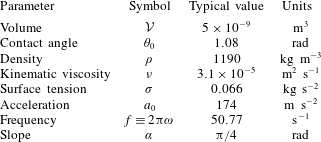
which are the dimensionless frequency of the oscillations and a scaled ratio of the gravitational acceleration to the applied acceleration. Table 1 shows some typical values of the physical parameters appropriate for the experiments of Brunet et al. (Reference Brunet, Eggers and Deegan2007). We will assume that a droplet with a volume of
 $5~\unicode[STIX]{x03BC}\text{l}$
has a length scale
 $D_{0}\approx 2~\text{mm}$
, which is the cube root of the volume and also the approximate capillary length. This leads to
 $$\begin{eqnarray}\unicode[STIX]{x1D716}\approx 8.1,\quad \unicode[STIX]{x1D6FE}\approx 1.08,\quad \hat{\unicode[STIX]{x1D714}}\approx 1.30,\quad {\hat{g}}\approx 2.75\times 10^{-2},\quad \unicode[STIX]{x1D703}_{0}\approx 1.08.\end{eqnarray}$$
In addition, we find that the Reynolds number, using
 $\unicode[STIX]{x1D714}D_{0}$
as the velocity scale, is
 $$\begin{eqnarray}Re={\displaystyle \frac{\unicode[STIX]{x1D714}D_{0}^{2}}{\unicode[STIX]{x1D708}}}\approx 41.2,\end{eqnarray}$$
which gives us reasonable grounds for neglecting viscous stresses. Note that the effect of viscosity on the contact line dynamics is not neglected; it is modelled through the function
 $v(\unicode[STIX]{x1D703})$
, and that the assumption of two-dimensionality is likely to have a more significant effect on our results than the neglect of the oscillating boundary layer on the solid surface.
Typical values for the parameters taken from Brunet et al. (Reference Brunet, Eggers and Deegan2007).

The final, dimensionless set of equations that we will study is, dropping hats for notational convenience,
 $$\begin{eqnarray}\unicode[STIX]{x1D6FB}^{2}\unicode[STIX]{x1D719}=0\quad \text{in }{\mathcal{D}}(t),\end{eqnarray}$$
subject to
 $$\begin{eqnarray}{\displaystyle \frac{\unicode[STIX]{x2202}\unicode[STIX]{x1D719}}{\unicode[STIX]{x2202}t}}+{\displaystyle \frac{1}{2}}|\unicode[STIX]{x1D735}\unicode[STIX]{x1D719}|^{2}+{\displaystyle \frac{\text{d}V_{s}}{\text{d}t}}x-{\displaystyle \frac{1}{\unicode[STIX]{x1D703}_{0}}}\unicode[STIX]{x1D705}+\unicode[STIX]{x1D716}a\left(X+{\displaystyle \frac{\unicode[STIX]{x1D6FE}}{\unicode[STIX]{x1D703}_{0}}}Y\right)=0\quad \text{on }\boldsymbol{x}=\boldsymbol{X}(s,t),\end{eqnarray}$$
 $$\begin{eqnarray}\boldsymbol{n}\boldsymbol{\cdot }{\displaystyle \frac{\text{d}\boldsymbol{x}}{\text{d}t}}={\displaystyle \frac{\unicode[STIX]{x2202}\unicode[STIX]{x1D719}}{\unicode[STIX]{x2202}n}}\quad \text{on }\boldsymbol{x}=\boldsymbol{X}(s,t),\end{eqnarray}$$
 $$\begin{eqnarray}{\displaystyle \frac{\unicode[STIX]{x2202}\unicode[STIX]{x1D719}}{\unicode[STIX]{x2202}y}}=0\quad \text{on }y=0,\end{eqnarray}$$
 $$\begin{eqnarray}{\displaystyle \frac{\text{d}D}{\text{d}t}}=v(\unicode[STIX]{x1D703}_{-})+V_{s},\quad y=0,\quad {\displaystyle \frac{\unicode[STIX]{x2202}\unicode[STIX]{x1D719}}{\unicode[STIX]{x2202}s}}=-{\displaystyle \frac{\text{d}D}{\text{d}t}}\cos \unicode[STIX]{x1D703}_{-}\quad \text{at }s=0,\end{eqnarray}$$
 $$\begin{eqnarray}{\displaystyle \frac{\text{d}D}{\text{d}t}}=v(\unicode[STIX]{x1D703}_{+})-V_{s},\quad y=0,\quad {\displaystyle \frac{\unicode[STIX]{x2202}\unicode[STIX]{x1D719}}{\unicode[STIX]{x2202}s}}={\displaystyle \frac{\text{d}D}{\text{d}t}}\cos \unicode[STIX]{x1D703}_{+}\quad \text{at }s=L.\end{eqnarray}$$
These equations must be solved for the position of the free surface,
 $\boldsymbol{X}(s,t)$
, the velocity potential,
 $\unicode[STIX]{x1D719}(x,y,t)$
, the half-width
 $D(t)$
and the velocity of the midpoint of the base of the drop,
 $V_{s}(t)$
, which we refer to as the velocity of the drop.
3 Asymptotic solution for small-amplitude forcing
 $(\unicode[STIX]{x1D716}\ll 1)$

In this section we will solve (2.17) to (2.22) in the limit of small forcing (
 $\unicode[STIX]{x1D716}\ll 1$
). The structure of this weakly nonlinear solution is the same as that described in Benilov & Billingham (Reference Benilov and Billingham2011), with the leading-order solution steady, the
 $O(\unicode[STIX]{x1D716})$
correction a combination of odd and even modes, and the leading-order rise velocity of the droplet of
 $O(\unicode[STIX]{x1D716}^{2})$
, fixed by considering an integral of the full problem. We are unable to study contact angle hysteresis using this approach, since the contact line remains pinned in the limit
 $\unicode[STIX]{x1D716}\rightarrow 0$
if
 $\unicode[STIX]{x1D703}_{A}>\unicode[STIX]{x1D703}_{R}$
. We therefore take
 $\unicode[STIX]{x1D703}_{A}=\unicode[STIX]{x1D703}_{R}\equiv \unicode[STIX]{x1D703}_{0}$
and Taylor-expand the contact line law close to equilibrium as
 $$\begin{eqnarray}v(\unicode[STIX]{x1D703}_{\pm })=v^{\prime }\left({\displaystyle \frac{\unicode[STIX]{x1D703}_{\pm }}{\unicode[STIX]{x1D703}_{0}}}-1\right)+{\displaystyle \frac{1}{2}}v^{\prime \prime }\left({\displaystyle \frac{\unicode[STIX]{x1D703}_{\pm }}{\unicode[STIX]{x1D703}_{0}}}-1\right)^{2}+\cdots \,,\end{eqnarray}$$
where
 $v^{\prime }$
and
 $v^{\prime \prime }$
are dimensionless constants, equivalent to the constants of the same name in Benilov & Billingham (Reference Benilov and Billingham2011).
At leading order as
 $\unicode[STIX]{x1D716}\rightarrow 0$
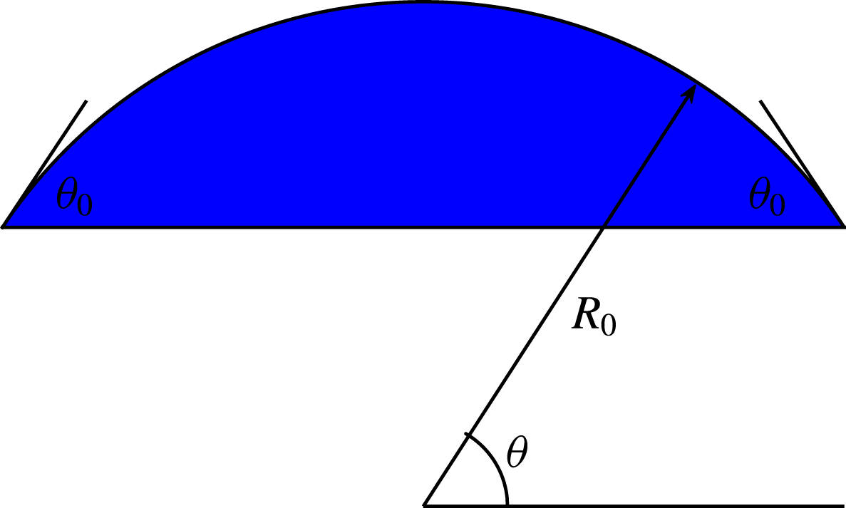
the droplet is at rest in equilibrium, with its free surface an arc of a circle. This means that the analysis is more straightforward in a polar coordinate system
 $(r,\unicode[STIX]{x1D703})$
, with this free surface centred at the origin at leading order, as shown in figure 2. Note that our choice of dimensionless parameters gives a droplet footprint of unit equilibrium half-width. The free surface of the droplet is now given by
 $r=R(\unicode[STIX]{x1D703},t)$
. We expand each unknown in powers of
 $\unicode[STIX]{x1D716}$
, for example,
 $R=R_{0}+\unicode[STIX]{x1D716}R_{1}+O(\unicode[STIX]{x1D716}^{2})$
as
 $\unicode[STIX]{x1D716}\rightarrow 0$
.
The leading-order position of the free surface in the polar coordinate system used in the asymptotic analysis when
 $\unicode[STIX]{x1D716}\ll 1$
.

The leading-order solution, which represents the droplet in the absence of any external forces, is
 $$\begin{eqnarray}\unicode[STIX]{x1D719}_{0}=-{\displaystyle \frac{\sin \unicode[STIX]{x1D703}_{0}}{\unicode[STIX]{x1D703}_{0}}}t,\quad R_{0}={\displaystyle \frac{1}{\sin \unicode[STIX]{x1D703}_{0}}},\quad V_{0}=0.\end{eqnarray}$$
We proceed by seeking a time-harmonic solution at
 $O(\unicode[STIX]{x1D716})$
and therefore define
 $$\begin{eqnarray}\unicode[STIX]{x1D719}_{1}=\text{Re}\{\tilde{\unicode[STIX]{x1D719}}\text{e}^{\text{i}\unicode[STIX]{x1D714}t}\},\quad V_{1}=\text{Re}\{\tilde{V}\text{e}^{\text{i}\unicode[STIX]{x1D714}t}\},\quad R_{1}=\text{Im}\{\tilde{R}\text{e}^{\text{i}\unicode[STIX]{x1D714}t}\},\quad D_{1}=\text{Im}\{\tilde{D}\text{e}^{\text{i}\unicode[STIX]{x1D714}t}\}.\end{eqnarray}$$
This leads to a linear boundary value problem set in the domain
 ${\mathcal{D}}_{0}$
occupied by the droplet at leading order,
 $$\begin{eqnarray}\unicode[STIX]{x1D6FB}^{2}\tilde{\unicode[STIX]{x1D719}}=0\quad \text{in }{\mathcal{D}}_{0},\end{eqnarray}$$
subject to
 $$\begin{eqnarray}\displaystyle & & \displaystyle \unicode[STIX]{x1D714}\tilde{\unicode[STIX]{x1D719}}+\unicode[STIX]{x1D714}\tilde{V}{\displaystyle \frac{\cos \unicode[STIX]{x1D703}}{\sin \unicode[STIX]{x1D703}_{0}}}+{\displaystyle \frac{\sin ^{2}\unicode[STIX]{x1D703}_{0}}{\unicode[STIX]{x1D703}_{0}}}\left({\displaystyle \frac{\unicode[STIX]{x2202}^{2}\tilde{R}}{\unicode[STIX]{x2202}\unicode[STIX]{x1D703}^{2}}}+\tilde{R}\right)\nonumber\\ \displaystyle & & \displaystyle \quad ={\displaystyle \frac{1}{\sin \unicode[STIX]{x1D703}_{0}}}\left[\cos \unicode[STIX]{x1D703}+{\displaystyle \frac{\unicode[STIX]{x1D6FE}}{\unicode[STIX]{x1D703}_{0}}}(\sin \unicode[STIX]{x1D703}-\cos \unicode[STIX]{x1D703}_{0})\right]\quad \text{on }r=R_{0},\end{eqnarray}$$
 $$\begin{eqnarray}\displaystyle & \displaystyle \unicode[STIX]{x1D714}\tilde{R}={\displaystyle \frac{\unicode[STIX]{x2202}\tilde{\unicode[STIX]{x1D719}}}{\unicode[STIX]{x2202}r}}\quad \text{on }r=R_{0}, & \displaystyle\end{eqnarray}$$
 $$\begin{eqnarray}\displaystyle & \displaystyle \tilde{R}=\sin \unicode[STIX]{x1D703}_{0}\,\tilde{D},\quad {\displaystyle \frac{\unicode[STIX]{x2202}\tilde{\unicode[STIX]{x1D719}}}{\unicode[STIX]{x2202}\unicode[STIX]{x1D703}}}=\mp \cot \unicode[STIX]{x1D703}_{0}\,\unicode[STIX]{x1D714}\tilde{D}\quad \text{at }\unicode[STIX]{x1D703}={\displaystyle \frac{\unicode[STIX]{x03C0}}{2}}\mp \unicode[STIX]{x1D703}_{0}, & \displaystyle\end{eqnarray}$$
 $$\begin{eqnarray}\displaystyle & \displaystyle v^{\prime }{\displaystyle \frac{\sin \unicode[STIX]{x1D703}_{0}}{\unicode[STIX]{x1D703}_{0}}}{\displaystyle \frac{\unicode[STIX]{x2202}\tilde{R}}{\unicode[STIX]{x2202}\unicode[STIX]{x1D703}}}-\text{i}\tilde{V}\pm \left(v^{\prime }{\displaystyle \frac{\sin \unicode[STIX]{x1D703}_{0}}{\unicode[STIX]{x1D703}_{0}}}\cos \unicode[STIX]{x1D703}_{0}-\text{i}\unicode[STIX]{x1D714}\right)\tilde{D}=0\quad \text{at }\unicode[STIX]{x1D703}={\displaystyle \frac{\unicode[STIX]{x03C0}}{2}}\mp \unicode[STIX]{x1D703}_{0}. & \displaystyle\end{eqnarray}$$
In the limit
 $\unicode[STIX]{x1D703}_{0}\rightarrow 0$
, (3.4) to (3.8) reduce to (3.26) to (3.31) in Benilov & Billingham (Reference Benilov and Billingham2011).
We will solve (3.4) to (3.8) numerically, but we can first reduce the geometrical complexity of this boundary value problem by conformally mapping to the upper half-plane using the transformation
 $$\begin{eqnarray}w=\left({\displaystyle \frac{1+z-\text{i}\cot \unicode[STIX]{x1D703}_{0}}{1-z+\text{i}\cot \unicode[STIX]{x1D703}_{0}}}\right)^{\unicode[STIX]{x03C0}/\unicode[STIX]{x1D703}_{0}},\end{eqnarray}$$
where
 $z=x+\text{i}y$
. The base of the droplet is mapped to the positive real axis and the surface of the droplet to the negative real axis with the contact line at
 $x=-1$
,
 $y=\cot \unicode[STIX]{x1D703}_{0}$
becoming the origin in the
 $w$
plane. It is now straightforward to solve for
 $\tilde{\unicode[STIX]{x1D719}}$
in the upper half-plane and eliminate it from the problem. This leads to the integral equation
 $$\begin{eqnarray}\displaystyle & & \displaystyle {\displaystyle \frac{\sin ^{3}\unicode[STIX]{x1D703}_{0}}{\unicode[STIX]{x1D703}_{0}}}\left({\displaystyle \frac{\unicode[STIX]{x2202}^{2}\tilde{R}}{\unicode[STIX]{x2202}\unicode[STIX]{x1D703}^{2}}}+\tilde{R}\right)-{\displaystyle \frac{\unicode[STIX]{x1D714}^{2}}{\unicode[STIX]{x03C0}}}\int _{\unicode[STIX]{x03C0}/2-\unicode[STIX]{x1D703}_{0}}^{\unicode[STIX]{x03C0}/2+\unicode[STIX]{x1D703}_{0}}\tilde{R}(\hat{\unicode[STIX]{x1D703}})\ln |u(\unicode[STIX]{x1D703})-u(\hat{\unicode[STIX]{x1D703}})|\,\text{d}\hat{\unicode[STIX]{x1D703}}+\unicode[STIX]{x1D714}\tilde{V}\cos \unicode[STIX]{x1D703}\nonumber\\ \displaystyle & & \displaystyle \quad =\cos \unicode[STIX]{x1D703}+{\displaystyle \frac{\unicode[STIX]{x1D6FE}}{\unicode[STIX]{x1D703}_{0}}}(\sin \unicode[STIX]{x1D703}-\cos \unicode[STIX]{x1D703}_{0})-\unicode[STIX]{x1D714}\unicode[STIX]{x1D719}_{\infty }\sin \unicode[STIX]{x1D703}_{0},\end{eqnarray}$$
for
 $\unicode[STIX]{x03C0}/2-\unicode[STIX]{x1D703}_{0}\leqslant \unicode[STIX]{x1D703}\leqslant \unicode[STIX]{x03C0}/2+\unicode[STIX]{x1D703}_{0}$
, where
 $$\begin{eqnarray}u(\unicode[STIX]{x1D703})=\left({\displaystyle \frac{\text{e}^{\text{i}\unicode[STIX]{x1D703}}-\text{i}\text{e}^{\text{i}\unicode[STIX]{x1D703}_{0}}}{\text{i}\text{e}^{-\text{i}\unicode[STIX]{x1D703}_{0}}-\text{e}^{\text{i}\unicode[STIX]{x1D703}}}}\right)^{\unicode[STIX]{x03C0}/\unicode[STIX]{x1D703}_{0}},\end{eqnarray}$$
and
 $\unicode[STIX]{x1D719}_{\infty }$
is a constant determined by the mass conservation condition
 $$\begin{eqnarray}\int _{\unicode[STIX]{x03C0}/2-\unicode[STIX]{x1D703}_{0}}^{\unicode[STIX]{x03C0}/2+\unicode[STIX]{x1D703}_{0}}\tilde{R}(\hat{\unicode[STIX]{x1D703}})\,\text{d}\hat{\unicode[STIX]{x1D703}}=0.\end{eqnarray}$$
The boundary conditions are
 $$\begin{eqnarray}\tilde{R}=\tilde{D}\sin \unicode[STIX]{x1D703}_{0},\quad {\displaystyle \frac{\unicode[STIX]{x2202}\tilde{R}}{\unicode[STIX]{x2202}\unicode[STIX]{x1D703}}}-{\displaystyle \frac{\text{i}\unicode[STIX]{x1D703}_{0}\tilde{V}}{v^{\prime }\sin \unicode[STIX]{x1D703}_{0}}}\pm \left(\cos \unicode[STIX]{x1D703}_{0}-{\displaystyle \frac{\text{i}\unicode[STIX]{x1D714}\unicode[STIX]{x1D703}_{0}}{v^{\prime }\sin \unicode[STIX]{x1D703}_{0}}}\right)\tilde{D}=0,\quad \text{at }\unicode[STIX]{x1D703}={\displaystyle \frac{\unicode[STIX]{x03C0}}{2}}\mp \unicode[STIX]{x1D703}_{0}.\end{eqnarray}$$
The solution of this integral equation can be separated into an odd part associated with
 $\tilde{V}$
(a swaying mode) and an even part associated with
 $\tilde{D}$
(a spreading mode), as was the case for
 $\unicode[STIX]{x1D703}_{0}\ll 1$
(Benilov & Billingham Reference Benilov and Billingham2011). We solve (3.10) to (3.13) using a finite difference discretisation, evaluating the integral using Simpson’s rule, whilst taking care to subtract out the weak singularities in the integrand where appropriate.
The final part of this asymptotic analysis involves the force balance on the droplet. In terms of the dimensionless velocity field,
 $\boldsymbol{u}\equiv (u,v)=\unicode[STIX]{x1D735}\unicode[STIX]{x1D719}$
, the
 $x$
component of the momentum equation is
 $$\begin{eqnarray}{\displaystyle \frac{\text{d}u}{\text{d}t}}+{\displaystyle \frac{\text{d}V_{s}}{\text{d}t}}=-{\displaystyle \frac{\unicode[STIX]{x2202}p}{\unicode[STIX]{x2202}x}}-\unicode[STIX]{x1D716}a.\end{eqnarray}$$
If we integrate this equation over the droplet and use Reynolds’ transport theorem along with incompressibility and the boundary conditions, we find that
 $$\begin{eqnarray}{\displaystyle \frac{\text{d}}{\text{d}t}}\left(\int _{{\mathcal{D}}}u\,\text{d}A+V_{s}A_{0}\right)={\displaystyle \frac{1}{\unicode[STIX]{x1D703}_{0}}}\int _{-x_{-}}^{x_{+}}n_{x}\unicode[STIX]{x1D705}\,\text{d}S-\unicode[STIX]{x1D716}aA_{0},\end{eqnarray}$$
where
 $A_{0}$
is the (constant) area of the droplet and
 $n_{x}$
is the
 $x$
component of the outward unit normal to the equilibrium free boundary. Averaging over a period of the oscillation eliminates the term on the left-hand side, and the integral on the right-hand side can be evaluated analytically to give
 $$\begin{eqnarray}\overline{\cos \unicode[STIX]{x1D703}_{+}}-\overline{\cos \unicode[STIX]{x1D703}_{-}}=\unicode[STIX]{x1D703}_{0}\unicode[STIX]{x1D716}\bar{a}A_{0},\end{eqnarray}$$
where the overbar represents the time average. Finally, if we rearrange (3.1) and substitute into the left-hand side, using the first-order asymptotic solutions for
 $D_{1}$
and
 $V_{1}$
, we are left with
 $$\begin{eqnarray}V_{r}=\unicode[STIX]{x1D716}^{2}\left[{\displaystyle \frac{\unicode[STIX]{x1D714}}{2v^{\prime }}}\left({\displaystyle \frac{v^{\prime \prime }}{v^{\prime }}}-\unicode[STIX]{x1D703}_{0}\cot \unicode[STIX]{x1D703}_{0}\right)\text{Re}(\tilde{V}\tilde{D}^{\ast })-{\displaystyle \frac{gv^{\prime }A_{0}}{2\sin \unicode[STIX]{x1D703}_{0}}}\right]+O(\unicode[STIX]{x1D716}^{3}),\end{eqnarray}$$
the leading-order approximation to the rise velocity of the droplet, which is of
 $O(\unicode[STIX]{x1D716}^{2})$
(a similar argument is used in Longuet-Higgins (Reference Longuet-Higgins1953, Reference Longuet-Higgins1983) and Lighthill (Reference Lighthill1978)). The first term depends linearly on frequency
 $\unicode[STIX]{x1D714}$
, nonlinearly on the contact line law through
 $v^{\prime }$
and
 $v^{\prime \prime }$
, and is driven by the relative phase of the spreading and swaying modes through the term
 $\text{Re}(\tilde{V}\tilde{D}^{\ast })$
. The second term is the sliding velocity of the droplet in the absence of the applied acceleration. This is qualitatively the same as (3.44) in Benilov & Billingham (Reference Benilov and Billingham2011) (and corrects a typographical error therein), which is recovered from (3.17) in the limit
 $\unicode[STIX]{x1D703}_{0}\rightarrow 0$
as
 $$\begin{eqnarray}V_{r}=\unicode[STIX]{x1D716}^{2}\left[{\displaystyle \frac{\unicode[STIX]{x1D714}}{2v^{\prime }}}\left({\displaystyle \frac{v^{\prime \prime }}{v^{\prime }}}-1\right)\text{Re}(\tilde{V}\tilde{D}^{\ast })-{\displaystyle \frac{gv^{\prime }}{3}}\right],\end{eqnarray}$$
which gives us some confidence in the accuracy of our analysis. We will discuss this linear solution in § 4.
4 Numerical solutions of the full problem
In this section we will outline the numerical method that we use to solve the full, nonlinear free boundary problem, given by (2.17) to (2.22), and discuss what we can learn about the dynamics of the droplet for a variety of contact line laws. In Bradshaw (Reference Bradshaw2016), a wide range of models for the moving contact line (choices of
 $v(\unicode[STIX]{x1D703})$
) is discussed in detail. In this paper, we will focus on three areas: a linear contact line law; the effect of contact angle hysteresis; and a time-dependent contact line law. Note also that in all of our numerical results the effect of gravity is small, leading simply to an additional mean downward velocity and little change to the shape of the free surface. Given that in the experiments of Brunet et al. (Reference Brunet, Eggers and Deegan2007) the applied acceleration is an order of magnitude greater than the acceleration due to gravity, this is entirely reasonable, and we will take
 $g=0$
below.
4.1 Numerical solution method
We represent the free surface using straight-line elements and solve Laplace’s equation using the boundary integral method with
 $\unicode[STIX]{x1D719}$
constant on each element (Pozrikidis Reference Pozrikidis2002). The tangential velocity of the boundary nodes is controlled by virtual springs chosen to keep the nodal spacing even (Billingham Reference Billingham2002). The curvature and slope of the free surface are calculated by fitting a circular arc through three adjacent boundary points. Fully implicit time stepping is used, which is necessary in order to move the contact lines at the prescribed contact line velocity,
 $v(\unicode[STIX]{x1D703})$
. The resulting nonlinear algebraic equations are solved at each time step using quasi-Newton iteration, with the solution at the previous time step as the initial guess. One further point to note is that the accumulation of small numerical error leads to a slow change in the area of the droplet, which is a conserved quantity of the motion. We correct for this by including a time-dependent source term on the right-hand side of Laplace’s equation, whose (small) strength is determined as part of the solution at each time step to keep the area of the droplet constant.
In order to compute periodic solutions, we solve an initial value problem with a time-dependent forcing that slowly increases to the required value of
 $\unicode[STIX]{x1D716}$
in order to avoid breakage of the droplet by the initial transient. We then continue time stepping until the solution has converged to a time-periodic form. Further details of this and all other aspects of the implementation can be found in Bradshaw (Reference Bradshaw2016).
4.2 Linear contact line law:
$\unicode[STIX]{x1D703}_{A}=\unicode[STIX]{x1D703}_{R}=\unicode[STIX]{x1D703}_{0}$
,
$v(\unicode[STIX]{x1D703})=v^{\prime }(\unicode[STIX]{x1D703}/\unicode[STIX]{x1D703}_{0}-1)$


A linear contact line law,
 $v(\unicode[STIX]{x1D703})=v^{\prime }(\unicode[STIX]{x1D703}/\unicode[STIX]{x1D703}_{0}-1)$
, is the simplest possible choice, characterised by the values of
 $v^{\prime }$
and
 $\unicode[STIX]{x1D703}_{0}$
alone. Whether or not this is a realistic approximation to the experimentally observed motion of a contact line, by studying it we are able to gain some insight into what controls the dynamics of the droplet. A point to note, however, is that when the amplitude,
 $\unicode[STIX]{x1D716}$
, of the applied acceleration is large enough, as well as the possibility of the droplet breaking through ejection of a satellite droplet (pinch-off) or the appearance of a dry patch (touchdown), the contact angle may reach either zero or
 $\unicode[STIX]{x03C0}$
. Whilst the former two cases may be physically realistic, the latter takes the contact angle well beyond the range where a linear contact line law is likely to be valid.
We begin by studying the behaviour of the droplet with different static contact angles by varying
 $\unicode[STIX]{x1D703}_{0}$
. We then consider the effect of changing the inclination of the substrate by varying
 $\unicode[STIX]{x1D6FE}$
and the mobility of the contact line by varying
 $v^{\prime }$
. In each case, we focus on the rise velocity of the droplet as a function of the forcing frequency and amplitude,
 $\unicode[STIX]{x1D714}$
and
 $\unicode[STIX]{x1D716}$
.
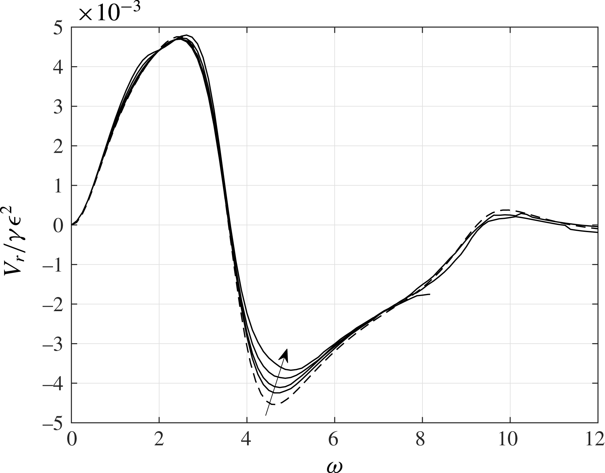
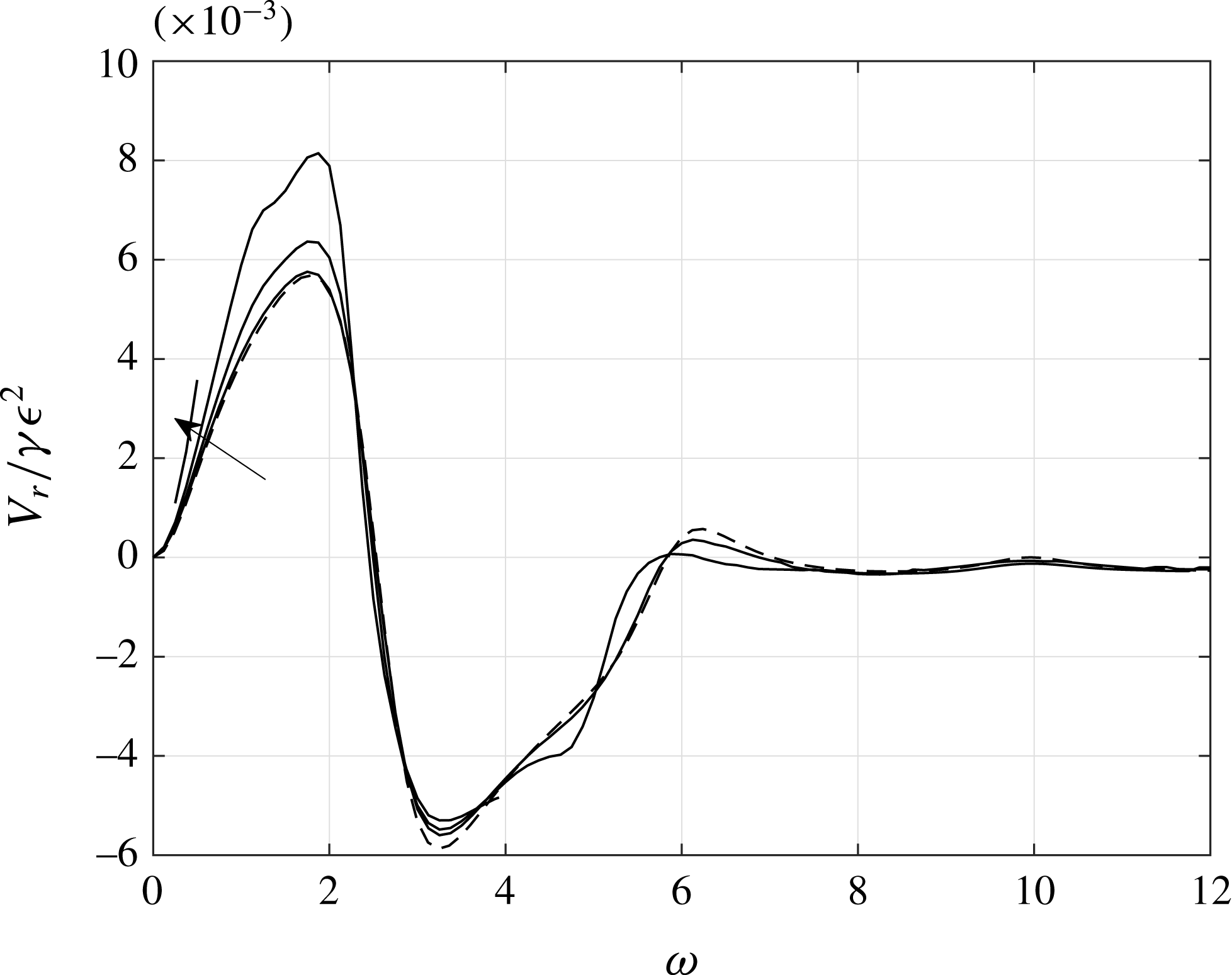
The rise velocity of the droplet as a function of
 $\unicode[STIX]{x1D714}$
for
 $\unicode[STIX]{x1D6FE}=5$
,
 $\unicode[STIX]{x1D703}_{0}=0.05$
,
 $v^{\prime }=0.5$
and no contact angle hysteresis. The dashed line is the asymptotic solution for
 $\unicode[STIX]{x1D716}\ll 1$
, whilst the solid lines, following the direction of the arrow, are for
 $\unicode[STIX]{x1D716}=0.25$
,
 $0.5$
,
 $0.75$
and
 $1$
. The results stop at
 $\unicode[STIX]{x1D714}=8.225$
for
 $\unicode[STIX]{x1D716}=0.75$
and at
 $\unicode[STIX]{x1D714}=6.975$
for
 $\unicode[STIX]{x1D716}=1$
because one of the contact angles reaches zero.

The rise velocity of the droplet as a function of
 $\unicode[STIX]{x1D714}$
for
 $\unicode[STIX]{x1D6FE}=5$
,
 $\unicode[STIX]{x1D703}_{0}=1$
,
 $v^{\prime }=0.5$
and no contact angle hysteresis. The dashed line is the asymptotic solution for
 $\unicode[STIX]{x1D716}\ll 1$
, whilst the solid lines, following the direction of the arrow, are for
 $\unicode[STIX]{x1D716}=0.25$
,
 $0.5$
,
 $0.75$
and
 $1$
, respectively. The results stop at
 $\unicode[STIX]{x1D714}=3.975$
for
 $\unicode[STIX]{x1D716}=0.75$
and at
 $\unicode[STIX]{x1D714}=0.55$
for
 $\unicode[STIX]{x1D716}=1$
because one of the contact angles reaches zero. In addition, the results for
 $\unicode[STIX]{x1D716}=1$
do not start until
 $\unicode[STIX]{x1D714}=0.25$
because the droplet pinches off for frequencies lower than this.

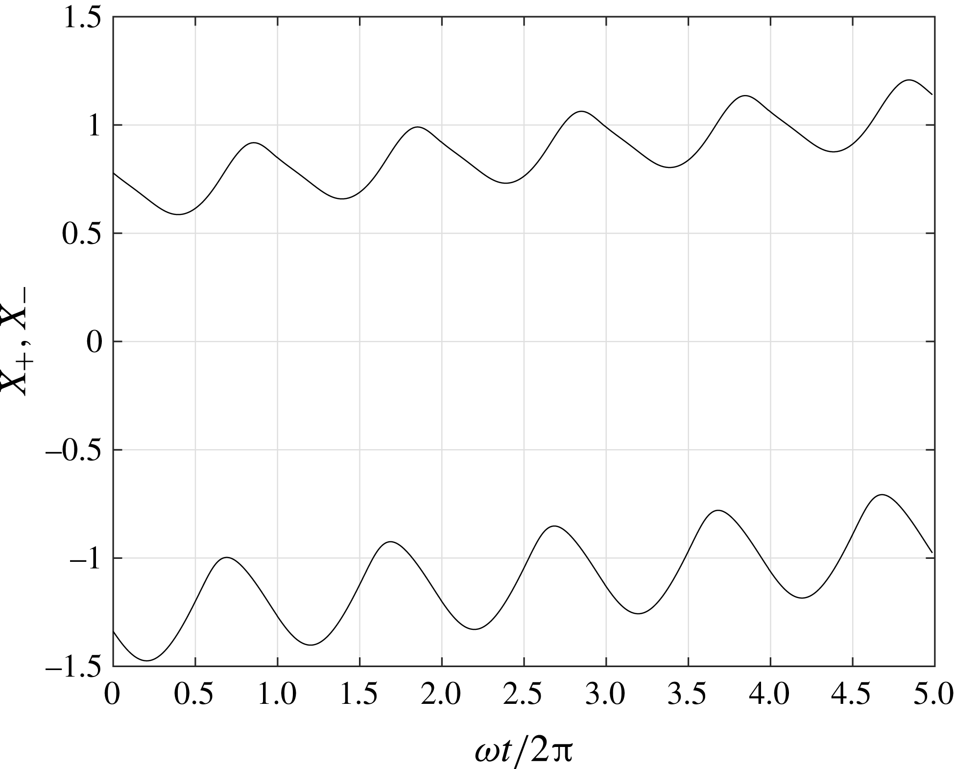
The position of the contact lines as a function of time for
 $\unicode[STIX]{x1D716}=0.75$
with the same parameters as those used in figure 4.

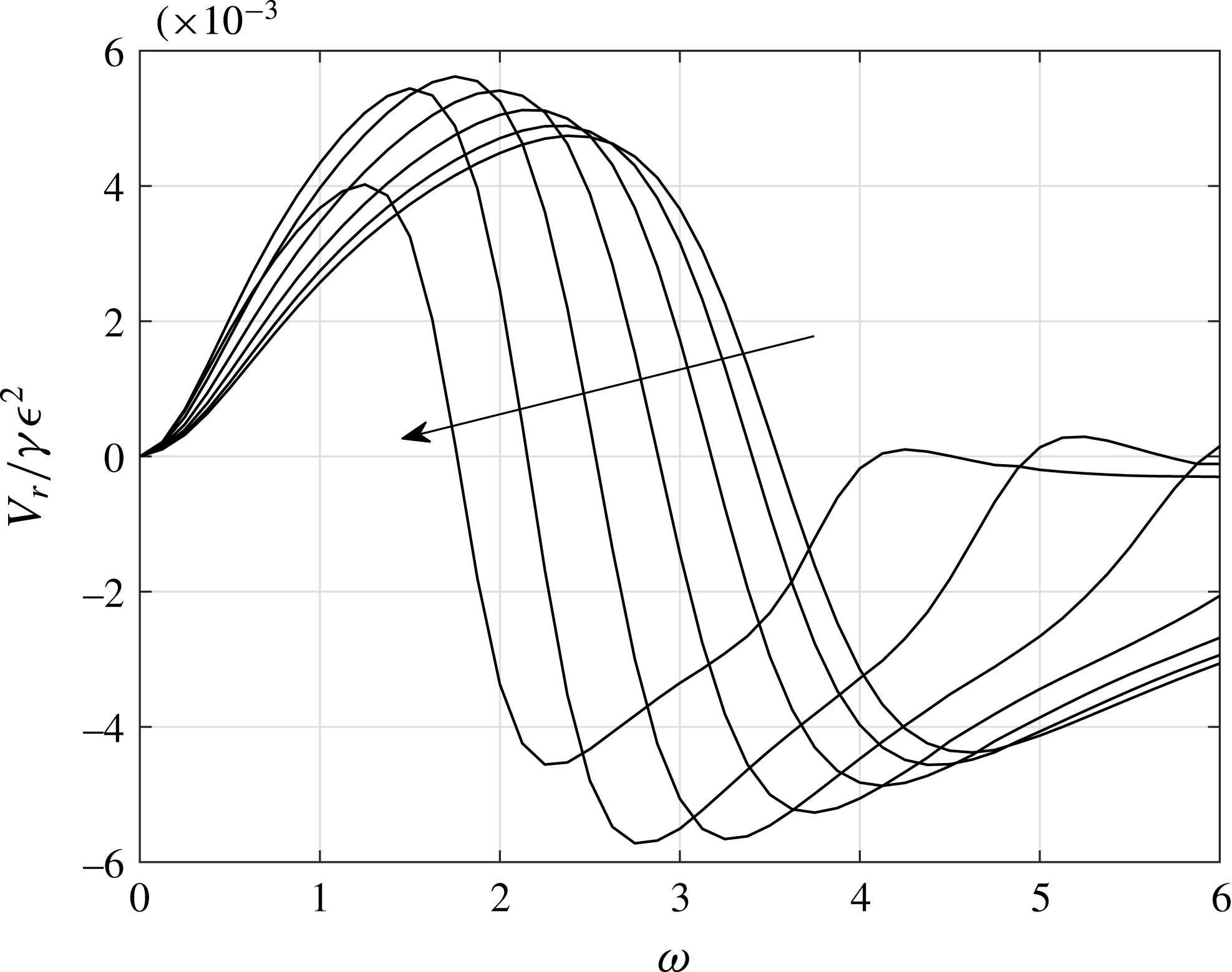
The rise velocity of the droplet as a function of
 $\unicode[STIX]{x1D714}$
for
 $\unicode[STIX]{x1D716}=0.1$
,
 $\unicode[STIX]{x1D6FE}=5$
,
 $v^{\prime }=0.5$
and no contact angle hysteresis. The
 $\unicode[STIX]{x1D703}_{0}$
value increases in the direction of the arrow, starting at 0.2 and increasing in multiples of 0.2.

The rise velocity of the droplet, calculated using the asymptotic solution for
 $\unicode[STIX]{x1D716}\ll 1$
, for
 $\unicode[STIX]{x1D6FE}=1$
,
 $v^{\prime }=0.5$
.

Snapshots of the shape of the droplet with
 $\unicode[STIX]{x1D716}=0.5$
,
 $\unicode[STIX]{x1D6FE}=1$
,
 $\unicode[STIX]{x1D714}=2$
,
 $v^{\prime }=0.5$
and
 $\unicode[STIX]{x1D703}_{0}=1$
,
 $2.2$
,
 $2.5$
,
 $2.65$
,
 $2.74$
,
 $2.8$
and
 $2.84$
. The filled graphs are numerical solutions of the full problem, whilst the unfilled graphs are drawn using the asymptotic solution for
 $\unicode[STIX]{x1D716}\ll 1$
.

4.2.1 The effect of varying the static contact angle,
$\unicode[STIX]{x1D703}_{0}$

Figure 3 shows how the rise velocity of the droplet varies with the frequency of the applied acceleration for
 $\unicode[STIX]{x1D703}_{0}=0.05$
and various values of
 $\unicode[STIX]{x1D716}$
. This reproduces the result presented in Benilov & Billingham (Reference Benilov and Billingham2011) for
 $\unicode[STIX]{x1D703}_{0}\ll 1$
, and also shows good agreement with the asymptotic solution for
 $\unicode[STIX]{x1D716}\ll 1$
(for values of
 $\unicode[STIX]{x1D716}$
smaller than
 $0.25$
, agreement with the asymptotic solution becomes progressively closer as
 $\unicode[STIX]{x1D716}$
decreases). As noted in Benilov & Billingham (Reference Benilov and Billingham2011), the small-
 $\unicode[STIX]{x1D716}$
asymptotic solution is in remarkably good agreement with the numerical solution of the full problem even when
 $\unicode[STIX]{x1D716}=1$
, with the rise velocity approximately proportional to
 $\unicode[STIX]{x1D716}^{2}$
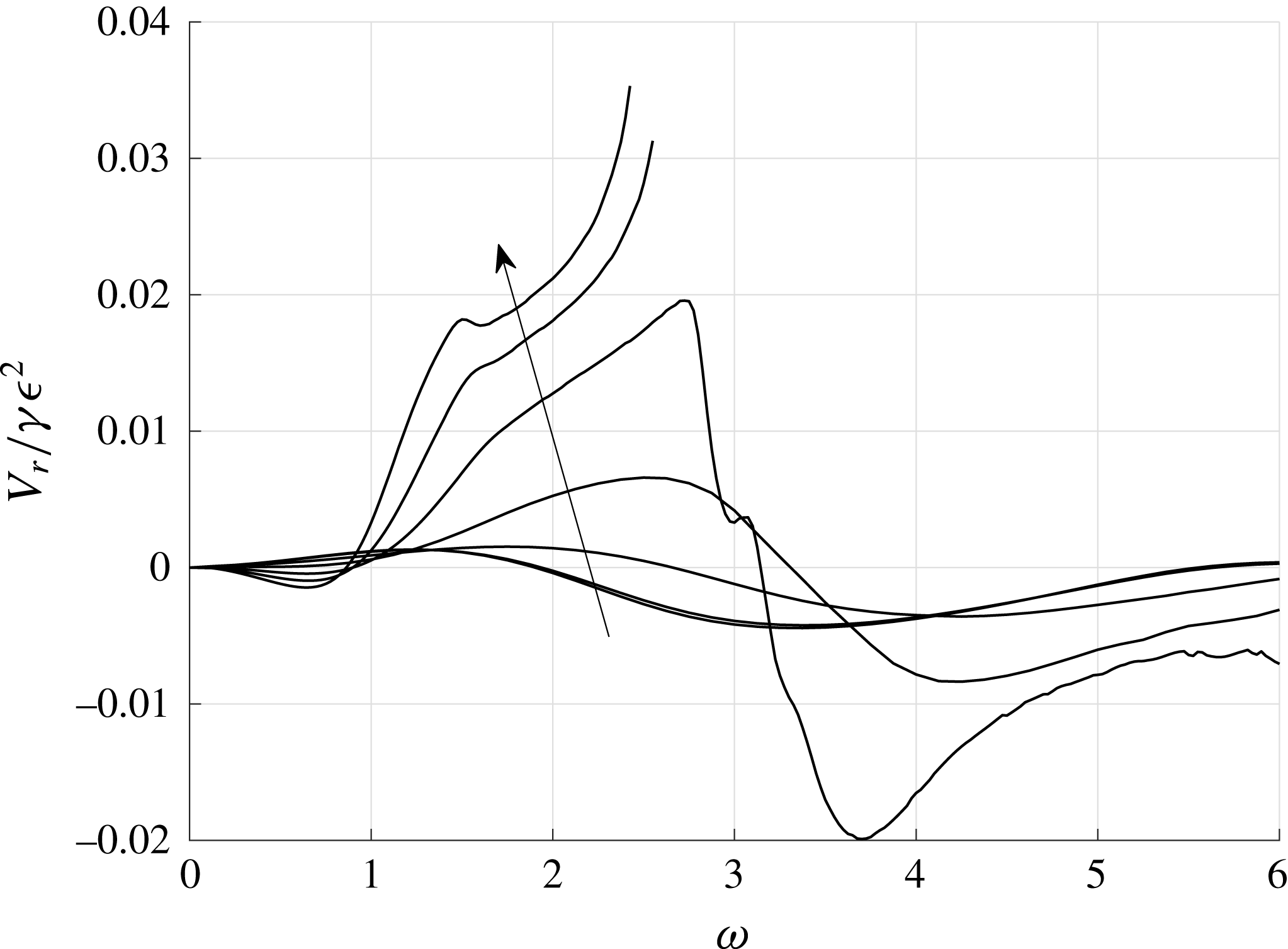
. We can see similar results in figure 4 for a larger static contact angle,
 $\unicode[STIX]{x1D703}_{0}=1$
. Although there is a somewhat larger deviation as
 $\unicode[STIX]{x1D716}$
grows, the rise velocity remains close to that predicted by the weakly nonlinear asymptotic solution for
 $\unicode[STIX]{x1D716}\ll 1$
and the qualitative behaviour is very similar to that shown in figure 3 for
 $\unicode[STIX]{x1D703}_{0}=0.05$
, with the droplet rising at lower frequencies of forcing, falling at higher frequencies, and remaining static (in the absence of gravity) as
 $\unicode[STIX]{x1D714}\rightarrow \infty$
. Figure 5 shows the position of the contact lines as a function of time for the parameter values used in figure 4. The rise of the droplet over each cycle of the driving acceleration is clearly visible. Figure 6 shows how the rise velocity changes as the static contact angle,
 $\unicode[STIX]{x1D703}_{0}$
, varies from
 $0.2$
to
 $1.4$
. The maximum rise velocity shifts to lower frequencies, and the value of this maximum increases slightly until
 $\unicode[STIX]{x1D703}_{0}\approx 1$
, then decreases. At
 $\unicode[STIX]{x1D703}_{0}=\unicode[STIX]{x03C0}/2$
, the rise velocity is zero at all frequencies, consistent with the asymptotic result (3.17) for
 $\unicode[STIX]{x1D716}\ll 1$
. For static contact angles greater than
 $\unicode[STIX]{x03C0}/2$
, the dynamics of the droplet starts to show very sensitive dependence on
 $\unicode[STIX]{x1D703}_{0}$
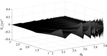
. Figure 7 shows the rise velocity of the droplet as a function of
 $\unicode[STIX]{x1D714}$
and
 $\unicode[STIX]{x1D703}_{0}$
, calculated from the asymptotic solution when
 $\unicode[STIX]{x1D716}\ll 1$
. We have verified as far as possible using numerical solutions of the full problem that the rapid oscillations shown are calculated correctly. We can explain this unexpectedly sensitive dependence of the rise velocity on the contact angle by noting that as
 $\unicode[STIX]{x1D703}_{0}\rightarrow \unicode[STIX]{x03C0}$
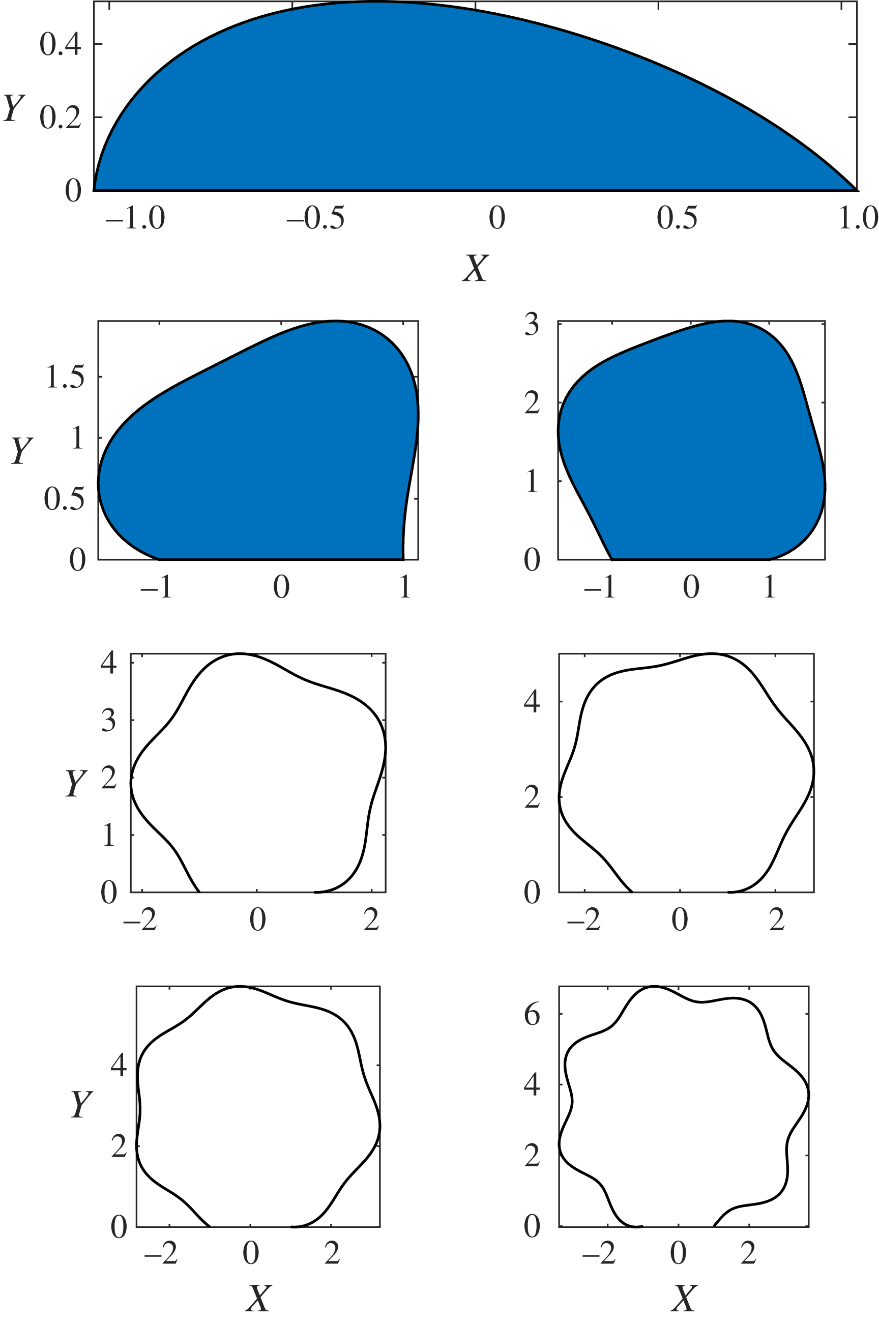
increasingly high-order harmonic modes of oscillation are excited on the surface of the droplet, as shown in figure 8. Although this complex interaction between the modes of oscillation of the droplet and the substrate is very interesting, it is also strongly dependent on the two-dimensional nature of our approximation (the fluid is really an oscillating cylinder), so we will not pursue it further here. However, this result does suggest that the dynamics of small droplets on oscillating, superhydrophobic surfaces is likely to be very complex, and worthy of further experimental and theoretical study.
4.2.2 The effect of varying the slope of the substrate,
$\unicode[STIX]{x1D6FE}^{-1}$

Equation (2.18) shows how the parameter
 $\unicode[STIX]{x1D6FE}$
controls the relative size of the tangential (
 $x$
) forcing and normal (
 $y$
) forcing terms, which control the swaying and spreading modes, respectively. Increasing the parameter
 $\unicode[STIX]{x1D716}$
varies both modes equally, whilst increasing
 $\unicode[STIX]{x1D6FE}$
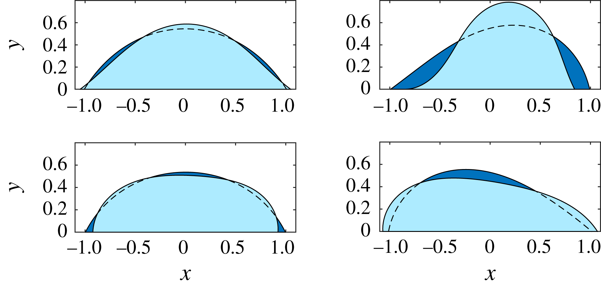
increases the amplitude of just the spreading mode. We can see this in the solutions shown in figure 9, where the solution for
 $\unicode[STIX]{x1D6FE}=10$
has a larger spreading component than that for
 $\unicode[STIX]{x1D6FE}=1$
. The effect of changing
 $\unicode[STIX]{x1D6FE}$
on the rise velocity of the droplet is comparable to that of changing
 $\unicode[STIX]{x1D716}$
, with the rise velocity proportional to
 $\unicode[STIX]{x1D6FE}$
, as shown in figure 10.
The oscillating droplet plotted at equal time intervals over one period of oscillation. The parameter values are
 $\unicode[STIX]{x1D716}=0.5$
,
 $\unicode[STIX]{x1D703}_{0}=1$
,
 $\unicode[STIX]{x1D714}=2$
,
 $v^{\prime }=0.5$
with no contact angle hysteresis. The droplets have
 $\unicode[STIX]{x1D6FE}=1$
for the darker shaded droplet and
 $\unicode[STIX]{x1D6FE}=10$
for the lighter shaded droplet.

The rise velocity of the droplet as a function of
 $\unicode[STIX]{x1D714}$
for
 $\unicode[STIX]{x1D716}=0.5$
,
 $\unicode[STIX]{x1D703}_{0}=1$
,
 $v^{\prime }=0.5$
and no contact angle hysteresis. The value of
 $\unicode[STIX]{x1D6FE}$
increases in the direction of the arrow, with
 $\unicode[STIX]{x1D6FE}=1$
,
 $5$
,
 $8$
and
 $10$
. The results stop at
 $\unicode[STIX]{x1D714}=4.125$
for
 $\unicode[STIX]{x1D6FE}=8$
and
 $\unicode[STIX]{x1D714}=2.125$
for
 $\unicode[STIX]{x1D6FE}=10$
due to one of the contact angles reaching zero.

4.2.3 The effect of varying the mobility of the contact line,
$v^{\prime }$

Varying
 $v^{\prime }$
, the contact line mobility, has a strong effect on the dynamics of the droplet. Note that, as
 $v^{\prime }\rightarrow 0$
, the contact line approaches complete pinning, and as
 $v^{\prime }\rightarrow \infty$
, the contact angle remains close to constant. Doubling
 $v^{\prime }$
from
 $0.5$
to
 $1$
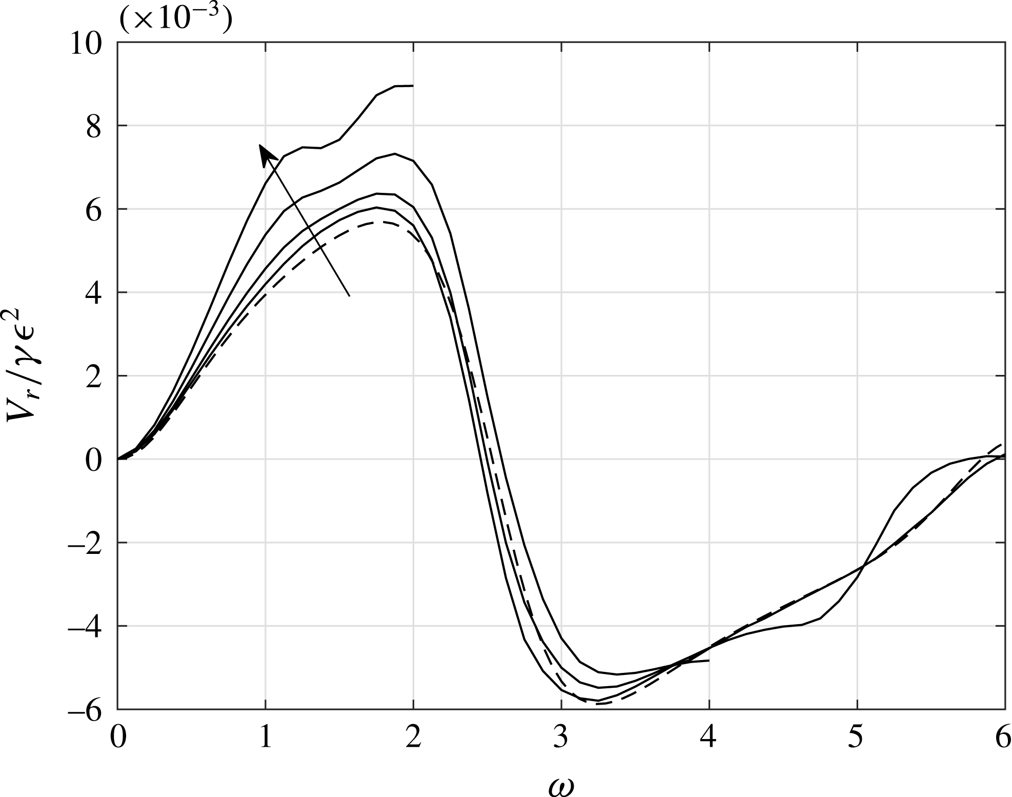
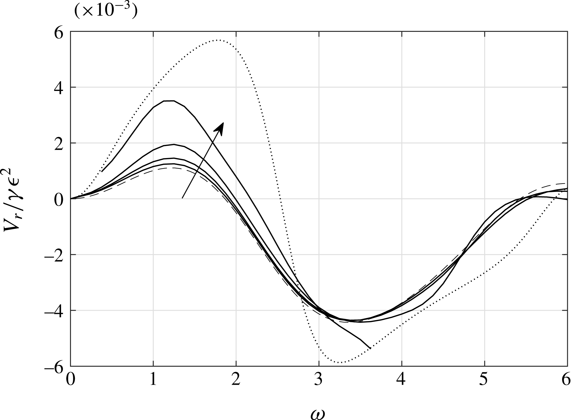
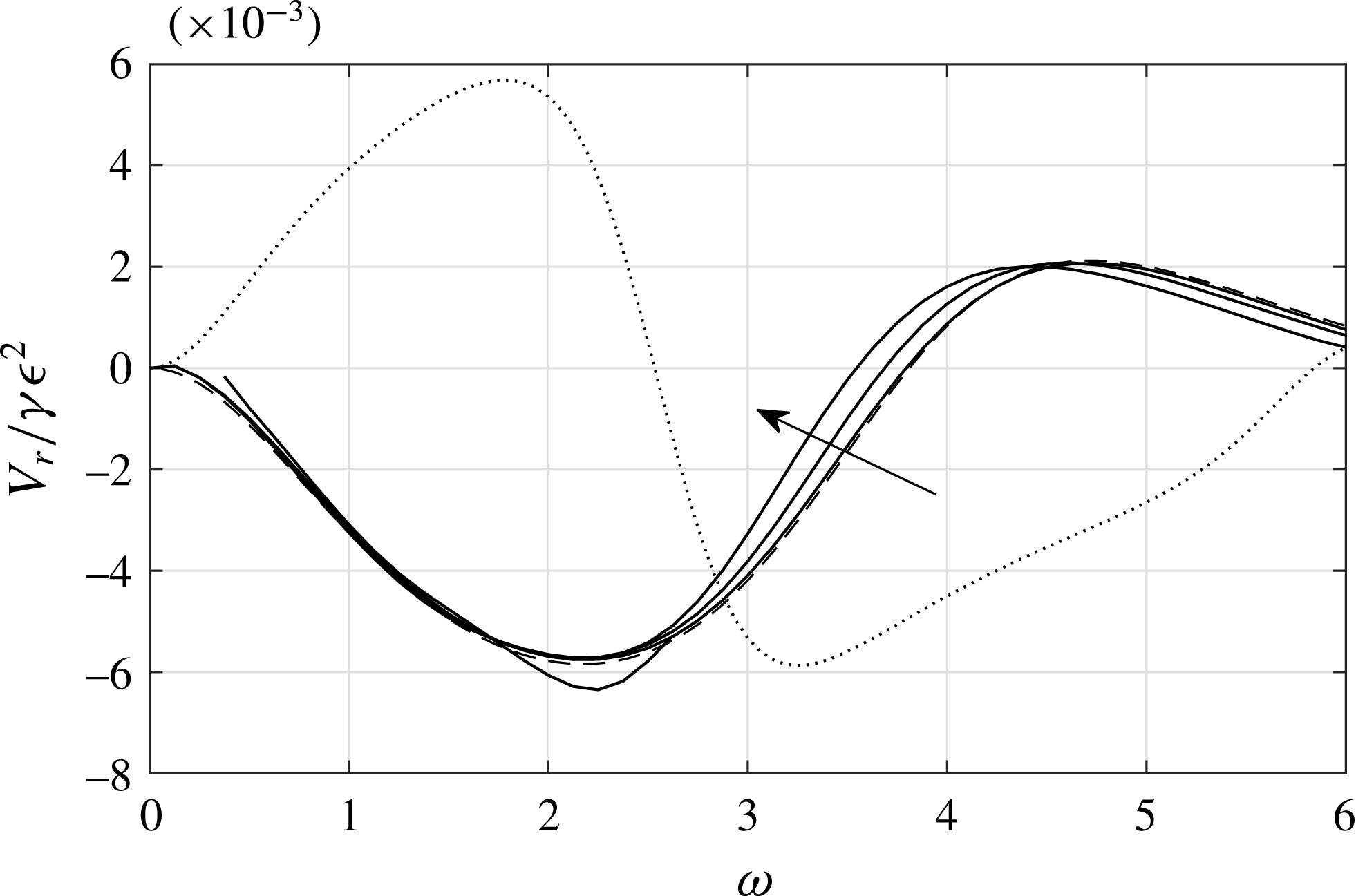
decreases the magnitude of the rise velocity, as shown in figure 11, and a further doubling to
 $2$
, as shown in figure 12, completely changes the sign, and hence the qualitative nature, of the rise velocity, although it continues to remain close to the asymptotic solution for
 $\unicode[STIX]{x1D716}\ll 1$
. Note also from (3.17) that, as
 $v^{\prime }\rightarrow \infty$
, the rise velocity for
 $\unicode[STIX]{x1D716}\ll 1$
is dominated by the downward component due to gravity (although we have set
 $g=0$
in all our simulations). There is no net dissipation over a full cycle of the oscillation at a contact line with constant contact angle since the constant tangential component of the surface tension force does no net work there.
The rise velocity of the droplet as a function of
 $\unicode[STIX]{x1D714}$
for
 $\unicode[STIX]{x1D6FE}=5$
,
 $\unicode[STIX]{x1D703}_{0}=1$
,
 $v^{\prime }=1$
and no contact angle hysteresis. The dashed line is the asymptotic solution for
 $\unicode[STIX]{x1D716}\ll 1$
, whilst the solid lines, following the direction of the arrow, have
 $\unicode[STIX]{x1D716}=0.25$
,
 $0.5$
,
 $0.75$
and
 $1$
. The dotted line is the asymptotic solution for
 $\unicode[STIX]{x1D716}\ll 1$
when
 $v^{\prime }=0.5$
. The results for
 $\unicode[STIX]{x1D716}=1$
do not start until
 $\unicode[STIX]{x1D714}=0.375$
due to the droplet pinching off, and stop at
 $\unicode[STIX]{x1D714}=3.75$
due to one of the contact angles reaching zero.

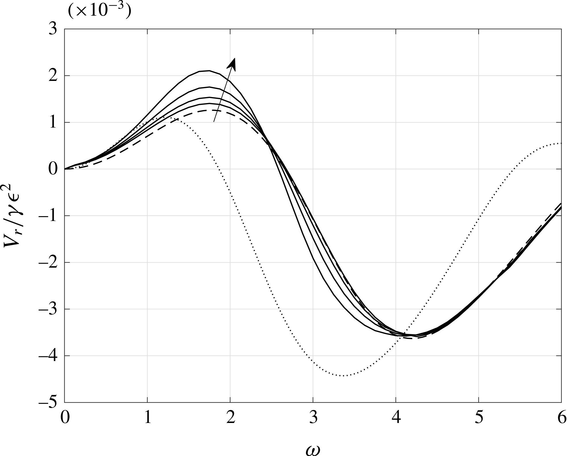
The rise velocity of the droplet as a function of
 $\unicode[STIX]{x1D714}$
for
 $\unicode[STIX]{x1D6FE}=5$
,
 $\unicode[STIX]{x1D703}_{0}=1$
,
 $v^{\prime }=2$
and no contact angle hysteresis. The dashed line is the asymptotic solution for
 $\unicode[STIX]{x1D716}\ll 1$
, whilst the solid lines, following the direction of the arrow, have
 $\unicode[STIX]{x1D716}=0.25$
,
 $0.5$
,
 $0.75$
and
 $1$
. The dotted line is the asymptotic solution for
 $\unicode[STIX]{x1D716}\ll 1$
when
 $v^{\prime }=0.5$
. The results for
 $\unicode[STIX]{x1D716}=1$
do not start until
 $\unicode[STIX]{x1D714}=0.375$
due to the droplet pinching off, and stop at
 $\unicode[STIX]{x1D714}=2.75$
due to one of the contact angles reaching zero.

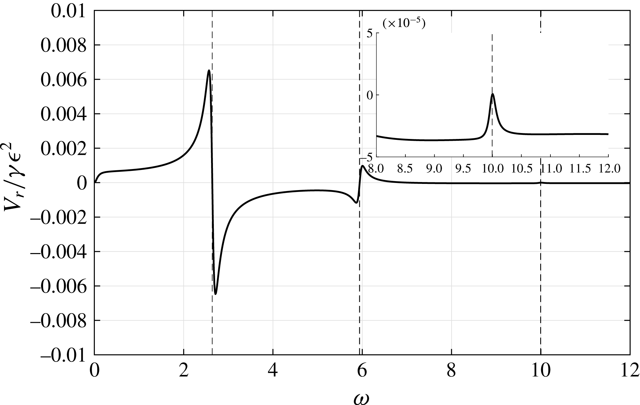
The asymptotic solution for
 $\unicode[STIX]{x1D716}\ll 1$
when
 $\unicode[STIX]{x1D6FE}=1$
,
 $\unicode[STIX]{x1D703}_{0}=1$
,
 $v^{\prime }=0.05$
and no contact angle hysteresis. The first three resonant frequencies for a pinned droplet are shown as broken lines.

In order to understand what happens when
 $v^{\prime }$
is small, and the droplet is close to pinned, consider the asymptotic solution for
 $\unicode[STIX]{x1D716}\ll 1$
with
 $v^{\prime }=0.05$
shown in figure 13. The rise velocity is close to zero, except for sharp spikes at a discrete set of frequencies. Since the contact lines are close to pinned, we would expect that these frequencies are close to the resonant frequencies of a completely pinned droplet. We can investigate this by solving (3.4) to (3.8), which control the small-amplitude oscillation of the droplet, after modifying the boundary conditions to those appropriate for pinned contact lines, which also has
 $\tilde{V}=\tilde{D}=0$
, to give
 $$\begin{eqnarray}\unicode[STIX]{x1D6FB}^{2}\tilde{\unicode[STIX]{x1D719}}=0~~\text{in }{\mathcal{D}}_{0},\end{eqnarray}$$
subject to
 $$\begin{eqnarray}\unicode[STIX]{x1D714}\tilde{\unicode[STIX]{x1D719}}+{\displaystyle \frac{\sin ^{2}\unicode[STIX]{x1D703}_{0}}{\unicode[STIX]{x1D703}_{0}}}\left({\displaystyle \frac{\unicode[STIX]{x2202}^{2}\tilde{R}}{\unicode[STIX]{x2202}\unicode[STIX]{x1D703}^{2}}}+\tilde{R}\right)={\displaystyle \frac{1}{\sin \unicode[STIX]{x1D703}_{0}}}\left(\cos \unicode[STIX]{x1D703}+{\displaystyle \frac{\unicode[STIX]{x1D6FE}}{\unicode[STIX]{x1D703}_{0}}}(\sin \unicode[STIX]{x1D703}-\cos \unicode[STIX]{x1D703}_{0})\right)\quad \text{at }r=R_{0},\end{eqnarray}$$
 $$\begin{eqnarray}\unicode[STIX]{x1D714}\tilde{R}={\displaystyle \frac{\unicode[STIX]{x2202}\tilde{\unicode[STIX]{x1D719}}}{\unicode[STIX]{x2202}r}}\quad \text{at }r=R_{0}\end{eqnarray}$$
and
 $$\begin{eqnarray}\tilde{R}=0,\quad {\displaystyle \frac{\unicode[STIX]{x2202}\tilde{\unicode[STIX]{x1D719}}}{\unicode[STIX]{x2202}\unicode[STIX]{x1D703}}}=0\quad \text{ at }\unicode[STIX]{x1D703}={\displaystyle \frac{\unicode[STIX]{x03C0}}{2}}\mp \unicode[STIX]{x1D703}_{0}.\end{eqnarray}$$
The
 $O(\unicode[STIX]{x1D716})$
correction to the time-dependent contact angles can be deduced from
 $$\begin{eqnarray}\unicode[STIX]{x1D703}_{\pm }=\unicode[STIX]{x1D703}_{0}\pm \unicode[STIX]{x1D716}\sin \unicode[STIX]{x1D703}_{0}{\displaystyle \frac{\unicode[STIX]{x2202}\tilde{R}}{\unicode[STIX]{x2202}\unicode[STIX]{x1D703}}}+O(\unicode[STIX]{x1D716}^{2})\quad \text{at }\unicode[STIX]{x1D703}={\displaystyle \frac{\unicode[STIX]{x03C0}}{2}}\mp \unicode[STIX]{x1D703}_{0}.\end{eqnarray}$$
The motion can still be decomposed into even (spreading) and odd (swaying) modes, which we can quantify by calculating
 $\unicode[STIX]{x1D703}_{+}+\unicode[STIX]{x1D703}_{-}$
and
 $\unicode[STIX]{x1D703}_{+}-\unicode[STIX]{x1D703}_{-}$
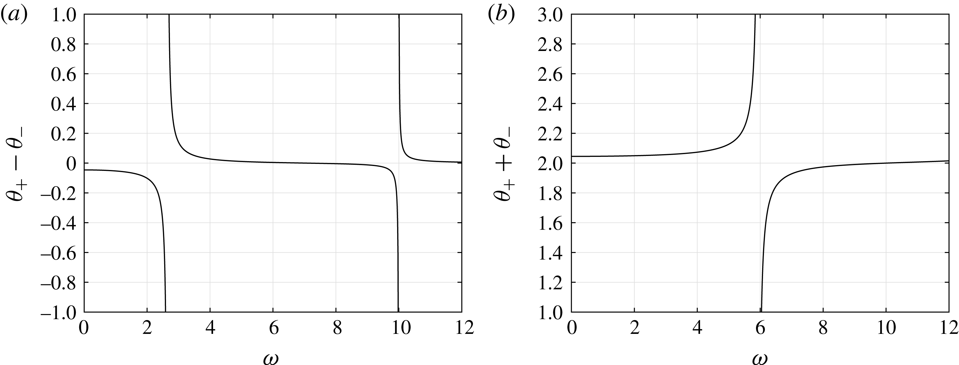
, respectively. Since pinned contact lines provide no damping, we expect to find a sequence of resonant frequencies, and these can indeed clearly be seen in figure 14. Comparison with figure 13 shows that the peaks in the magnitude of the rise velocity of the droplet when
 $v^{\prime }$
is small do indeed coincide with these resonant frequencies.
Measures of the magnitude of the odd (a) and even (b) modes as a function of
 $\unicode[STIX]{x1D714}$
for
 $\unicode[STIX]{x1D6FE}=5$
,
 $\unicode[STIX]{x1D703}_{0}=1$
and pinned contact lines. Resonant frequencies appear as singularities in these plots.

For the case of a linear contact line law, we have found that the rise velocity of the droplet is close to proportional to
 $\unicode[STIX]{x1D6FE}\unicode[STIX]{x1D716}^{2}$
even when
 $\unicode[STIX]{x1D716}$
is not small. Results for nonlinear contact line laws without hysteresis (see Bradshaw (Reference Bradshaw2016) for more details) suggest that this is mainly due to the linearity of the contact line law. In addition,
 $v^{\prime }$
, the mobility of the contact line, and
 $\unicode[STIX]{x1D703}_{0}$
, the static contact angle, have a strongly nonlinear effect on the rise velocity. Overall, this suggests that the model that we use for the motion of the contact line has the most effect on the dynamics of the droplet.
4.3 Hysteresis
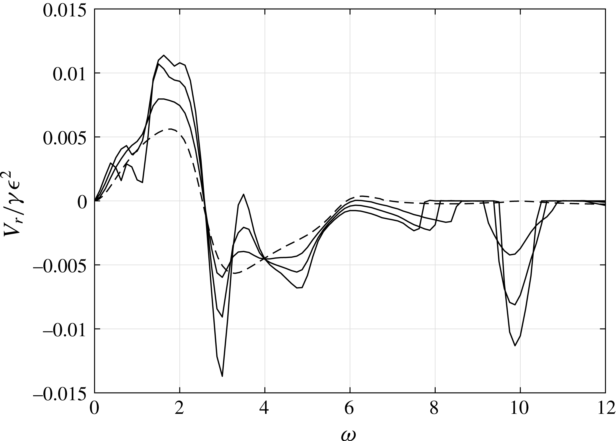
Figure 15 shows the effect of various non-zero hysteresis intervals
 $\unicode[STIX]{x1D703}_{I}\equiv \unicode[STIX]{x1D703}_{A}-\unicode[STIX]{x1D703}_{R}$
on the rise velocity of the droplet. The presence of odd resonant frequencies close to
 $\unicode[STIX]{x1D714}=3$
and
 $\unicode[STIX]{x1D714}=10$
has a strong effect on the rise velocity. The effect of the even mode close to
 $\unicode[STIX]{x1D714}=6$
is less striking. The maximum rise velocity is significantly increased by hysteresis, but close to
 $\unicode[STIX]{x1D714}=10$
the resonance leads to a sliding droplet. We can examine the effect of hysteresis on the rise velocity in more detail by fixing
 $\unicode[STIX]{x1D714}$
and varying
 $\unicode[STIX]{x1D703}_{I}$
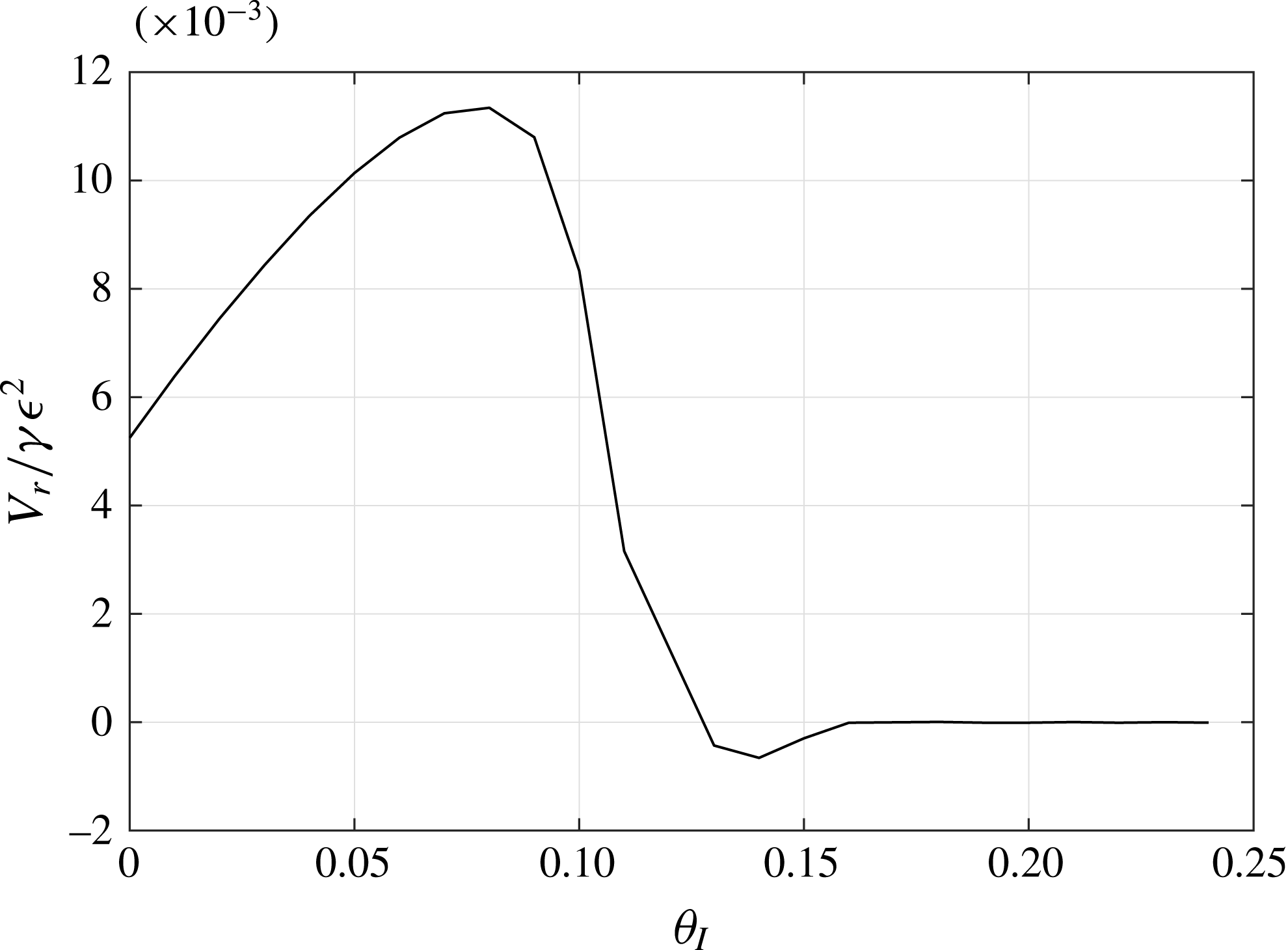
, as shown in figure 16. The rise velocity increases by a factor of more than two from its value when
 $\unicode[STIX]{x1D703}_{I}=0$
, but for large enough
 $\unicode[STIX]{x1D703}_{I}$
the droplet is completely pinned to the substrate. Note also that, although it is a priori possible that the rise velocity of the drop is related in a simple manner to the relative amplitudes of the spreading and swaying modes, in each of the cases discussed above a close examination of the numerical solutions does not provide any conclusive evidence for this (see Bradshaw (Reference Bradshaw2016) for a discussion).
The rise velocity of the droplet as a function of
 $\unicode[STIX]{x1D714}$
for
 $\unicode[STIX]{x1D716}=0.1$
,
 $\unicode[STIX]{x1D6FE}=5$
,
 $\unicode[STIX]{x1D703}_{0}=1$
and
 $v^{\prime }=0.5$
. The dashed line is the rise velocity in the absence of contact angle hysteresis, whilst the solid lines are the results for hysteresis intervals of 0.02, 0.04 and 0.06.

The rise velocity of the droplet as a function of the hysteresis interval for
 $\unicode[STIX]{x1D716}=0.1$
,
 $\unicode[STIX]{x1D6FE}=5$
,
 $\unicode[STIX]{x1D703}_{0}=1$
,
 $\unicode[STIX]{x1D714}=2$
and
 $v^{\prime }=0.5$
.

4.4 Time-dependent contact line law
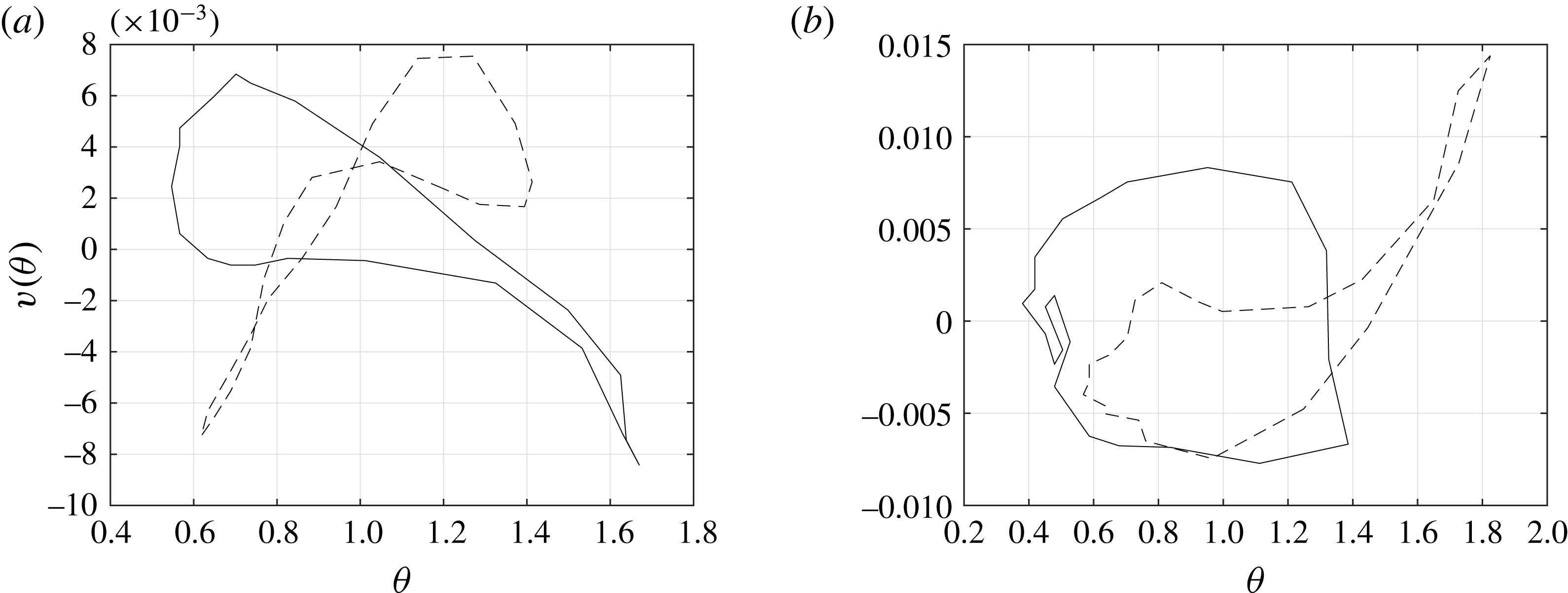
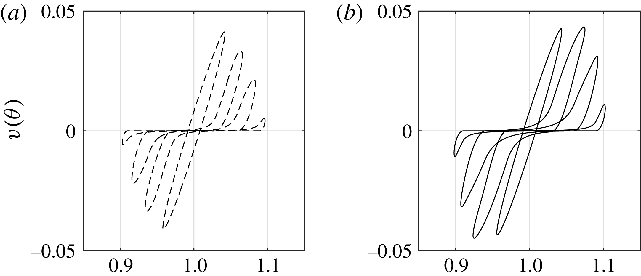
Figure 17 shows velocities of the leading and trailing contact points measured in the experiments of Brunet et al. (Reference Brunet, Eggers and Deegan2007) plotted as a function of measured apparent contact angle for both a sliding and a climbing droplet. The most striking feature of these graphs is that the contact line velocity is not a single-valued function of the apparent contact angle. Similar results can be found in Ting & Perlin (Reference Ting and Perlin1995) and Jiang et al. (Reference Jiang, Perlin and Schultz2004). Although it could be argued that the actual microscopic contact angle is a single-valued function of contact line velocity (most likely a constant), and that the behaviour of the apparent measured contact angle is influenced by both viscous bending and inertia close to the contact line, this does not help us within the traditional modelling framework that we have adopted here, where all the physics of the contact line is bundled into a model that gives contact line velocity as a function of contact angle. This leads us to propose that it is of interest to investigate the simplest possible time-dependent contact line law, namely
 $$\begin{eqnarray}\unicode[STIX]{x1D70F}{\displaystyle \frac{\text{d}V}{\text{d}t}}+V=v(\unicode[STIX]{x1D703}),\end{eqnarray}$$
where
 $V(t)$
is the velocity of the contact line,
 $v(\unicode[STIX]{x1D703})$
is a prescribed, single-valued function of the contact angle
 $\unicode[STIX]{x1D703}$
and
 $\unicode[STIX]{x1D70F}$
is the constant time scale over which the contact line velocity adjusts. The actual velocity of the contact line will lag behind the prescribed velocity,
 $v(\unicode[STIX]{x1D703})$
. When
 $\unicode[STIX]{x1D70F}=0$
, we recover the standard form of the contact line law. Note that (4.6) can also be written as
 $$\begin{eqnarray}V(t)={\displaystyle \frac{1}{\unicode[STIX]{x1D70F}}}\text{e}^{-t/\unicode[STIX]{x1D70F}}\int _{0}^{t}\text{e}^{s/\unicode[STIX]{x1D70F}}v(\unicode[STIX]{x1D703}(s))\,\text{d}s+\text{e}^{-t/\unicode[STIX]{x1D70F}}V(0).\end{eqnarray}$$
The velocity of the leading and trailing contact points as a function of the measured apparent contact angles, taken from the experiments of Brunet et al. (Reference Brunet, Eggers and Deegan2007). Panel (a) is for a sliding droplet and panel (b) is for a climbing droplet. The dashed lines are
 $\unicode[STIX]{x1D703}_{+}$
and the solid lines are
 $\unicode[STIX]{x1D703}_{-}$
.

The rise velocity of the droplet as a function of
 $\unicode[STIX]{x1D714}$
for
 $\unicode[STIX]{x1D6FE}=1$
,
 $\unicode[STIX]{x1D703}_{0}=1$
,
 $v^{\prime }=1$
and
 $\unicode[STIX]{x1D70F}=0.1$
. The dashed line is the asymptotic solution for
 $\unicode[STIX]{x1D716}\ll 1$
, whilst the solid lines, following the direction of the arrow, have
 $\unicode[STIX]{x1D716}=0.25$
,
 $0.5$
,
 $0.75$
and
 $1$
. The dotted line is the small-amplitude asymptotic solution for
 $\unicode[STIX]{x1D70F}=0$
.

The velocity of the contact lines as a function of contact angle for the time-dependent contact line law with
 $\unicode[STIX]{x1D70F}=0.1$
and
 $v^{\prime }=1$
. Panel (a) is for
 $\unicode[STIX]{x1D714}=1$
and panel (b) is for
 $\unicode[STIX]{x1D714}=6$
. The dashed line is
 $\unicode[STIX]{x1D703}_{+}$
and the solid line is
 $\unicode[STIX]{x1D703}_{-}$
.

The rise velocity of the droplet as a function of
 $\unicode[STIX]{x1D714}$
for
 $\unicode[STIX]{x1D716}=0.5$
,
 $\unicode[STIX]{x1D6FE}=1$
,
 $\unicode[STIX]{x1D703}_{0}=1$
and
 $v^{\prime }=1$
for the time-dependent contact line law. The solid lines, following the direction of the arrow, have
 $\unicode[STIX]{x1D70F}=0$
,
 $0.01$
,
 $0.1$
,
 $0.25$
,
 $0.5$
,
 $0.75$
and
 $1$
.

The rise velocity of the droplet as a function of
 $\unicode[STIX]{x1D714}$
for
 $\unicode[STIX]{x1D716}=0.1$
,
 $\unicode[STIX]{x1D6FE}=1$
,
 $\unicode[STIX]{x1D703}_{0}=1$
and
 $\unicode[STIX]{x1D70F}=0.1$
. The dashed line is the rise velocity when there is no contact angle hysteresis, whilst the solid lines have a hysteresis interval of
 $0.02$
,
 $0.04$
and
 $0.06$
.

The velocity of the contact lines as functions of contact angle for
 $\unicode[STIX]{x1D714}=2$
and
 $\unicode[STIX]{x1D70F}=0.1$
. Panel (a) shows
 $\unicode[STIX]{x1D703}_{+}$
and panel (b) shows
 $\unicode[STIX]{x1D703}_{-}$
. The hysteresis interval is
 $0$
,
 $0.02$
,
 $0.04$
and
 $0.06$
.

It is straightforward to include (4.6) in the weakly nonlinear analysis for
 $\unicode[STIX]{x1D716}\ll 1$
presented in § 3 and find that
 $$\begin{eqnarray}V_{r}=\unicode[STIX]{x1D716}^{2}\left[{\displaystyle \frac{\unicode[STIX]{x1D714}\left(1+\unicode[STIX]{x1D714}^{2}\unicode[STIX]{x1D70F}^{2}\right)}{2v^{\prime }}}\left({\displaystyle \frac{v^{\prime \prime }}{v^{\prime }}}-\unicode[STIX]{x1D703}_{0}\cot \unicode[STIX]{x1D703}_{0}\right)\text{Re}(\tilde{V}\tilde{D}^{\ast })-{\displaystyle \frac{gv^{\prime }A_{0}}{2\sin \unicode[STIX]{x1D703}_{0}}}\right]+O(\unicode[STIX]{x1D716}^{3}).\end{eqnarray}$$
Some results for an unsteady, linear contact line model are shown in figure 18. Although the rise velocity remains close to proportional to
 $\unicode[STIX]{x1D716}^{2}$
, increasing
 $\unicode[STIX]{x1D70F}$
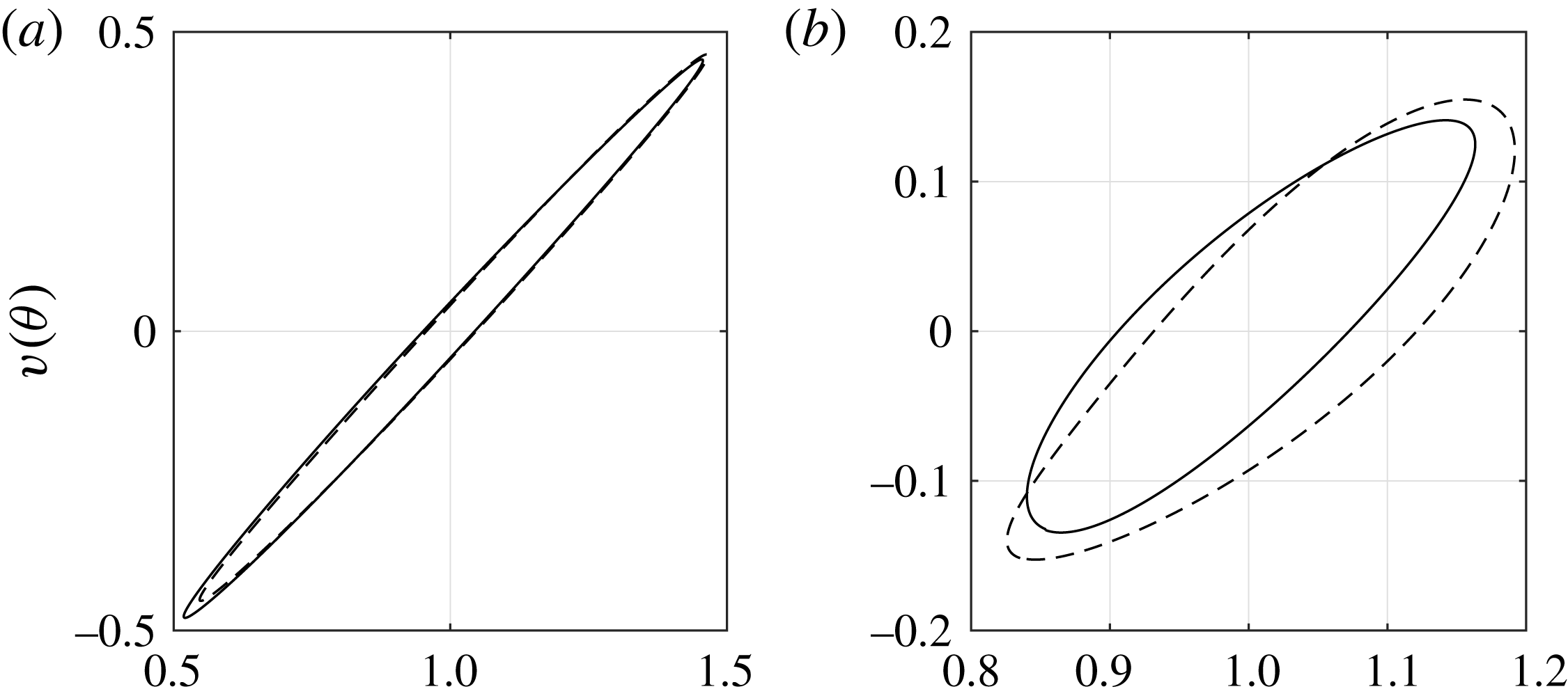
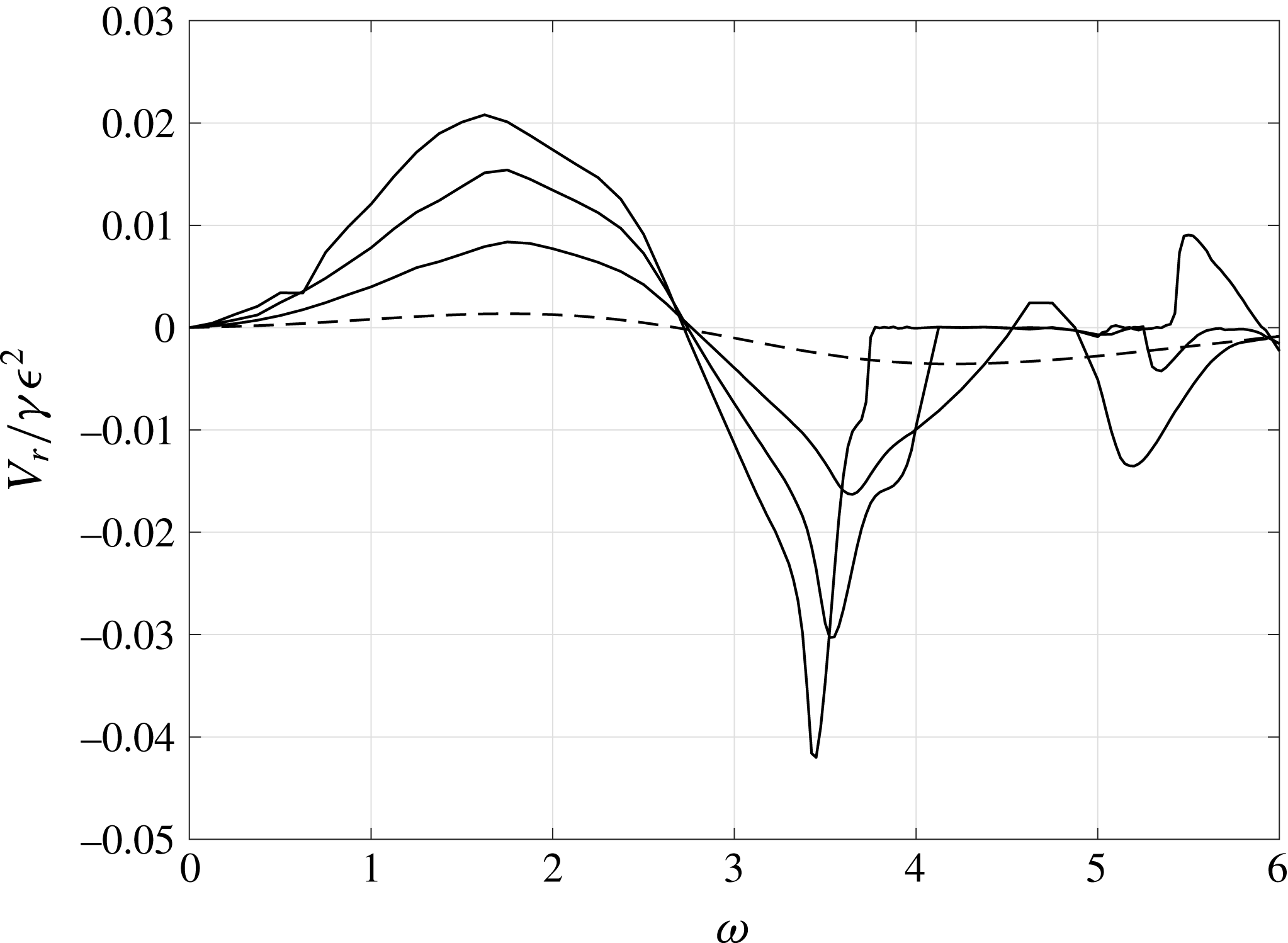
strongly affects the rise velocity, in particular making the maximum rise velocity significantly larger. Figure 19 shows how the contact line velocities vary with contact angle. As expected, this is no longer a simple, single-valued relationship and takes the form of an ellipse for
 $\unicode[STIX]{x1D716}\ll 1$
. Figure 20 shows how the rise velocity varies as
 $\unicode[STIX]{x1D70F}$
increases. When
 $\unicode[STIX]{x1D70F}$
is not small, the effect on the rise velocity is dramatic. For the two largest values of
 $\unicode[STIX]{x1D70F}$
shown, the graph terminates at finite
 $\unicode[STIX]{x1D714}$
because one of the contact angles reaches zero. Figure 21 shows that the inclusion of hysteresis in the unsteady contact line model has an even stronger effect, even more significant than the effect for the steady contact line law with hysteresis. Figure 22 shows how the behaviour of the contact line velocity as a function of contact angle is distorted by the presence of hysteresis. Finally, note that, although we have used a variety of different contact line laws, we have been unable to qualitatively reproduce the experimentally observed behaviour of the contact lines, although we note that our results are consistent with a droplet climbing up the plane when
 $\unicode[STIX]{x1D714}\approx 1$
.
5 Conclusion
In this paper we studied a two-dimensional, inviscid model of the motion of a droplet on a solid plane that is strongly oscillating in the vertical direction. This is the extension to arbitrary static contact angles of the work of Benilov & Billingham (Reference Benilov and Billingham2011). For small-amplitude forcing with a linear contact line law, we were able to find an asymptotic solution. In all other cases, we solved the free boundary problem numerically, using the boundary integral method. In each case, we found that the behaviour of the contact lines dominates the motion of the droplet. By varying the model used for the contact line velocity as a function of the apparent contact angle, we were able to study a wide variety of qualitatively different responses to the external forcing. As was found for the case of small contact angles, when the forcing is small and there is no contact angle hysteresis, the motion of the droplet is controlled by the weakly nonlinear interaction of swaying and spreading modes. For a linear contact line law, the weakly nonlinear form of the rise velocity remains a remarkably good approximation to the solution when the forcing parameter,
 $\unicode[STIX]{x1D716}$
, is of
 $O(1)$
. In this case, the contact line mobility,
 $v^{\prime }$
, has a strong effect on the rise velocity. We also studied the effect of contact angle hysteresis, which, as long as the hysteresis interval is not too large, can increase the rise velocity of the droplet due to the effect of the resonant modes of a fully pinned droplet.
Since the contact line velocity is not observed to be a single-valued function of the apparent contact angle in the experiments of Brunet et al. (Reference Brunet, Eggers and Deegan2007), we also studied a simple model for the motion of the contact line that has a memory over a time scale
 $\unicode[STIX]{x1D70F}$
. We found that the rise velocity is significantly increased when
 $\unicode[STIX]{x1D70F}$
is non-zero, particularly in the presence of contact angle hysteresis, and that the contact line velocity is indeed not a single-valued function of apparent contact angle when using this model in our simulations. We were, however, unable to reproduce the qualitative form of this dependence beyond noting that we obtain closed curves in graphs of contact line velocity as a function of contact angle. Given the simplicity of our modelling approach, this is perhaps not surprising. When Benilov (Reference Benilov2011) extended his earlier model from two to three dimensions, he found significant qualitative differences in the behaviour of the system. The obvious next step in this work is to extend the model studied here from two to three dimensions.