


Temnospondyli are the taxonomically most speciose, ecologically most diverse, and stratigraphically longest ranging group of early tetrapods, with a worldwide geographic distribution and an extensive fossil record spanning more than 200 Myr, from the Viséan (early Carboniferous) to the Aptian (upper Lower Cretaceous) (Milner Reference Milner and Benton1988, Reference Milner, Taylor and Larwood1990; Milner & Sequeira Reference Milner, Sequeira, Rolfe, Clarkson and Panchen1994; Warren et al. Reference Warren, Rich and Vickers-Rich1997; Schoch & Milner Reference Schoch and Milner2000, Reference Schoch and Milner2014; Carroll Reference Carroll2009; Clack Reference Clack2012; Schoch Reference Schoch2014a; Wagstaff et al. Reference Wagstaff, Gallagher, Hall, Korasidis, Rich, Seegets-Villiers and Vickers-Rich2020). They are readily distinguished from other early tetrapods by a unique combination of skeletal characteristics, including (but not limited to) broad and flat vomers, rigid sutures between exoccipitals, postparietals, and tabulars, and a pair of conspicuous, rounded openings on the palate. These openings, or interpterygoid vacuities, are slightly to much larger than the orbits (Witzmann & Ruta Reference Witzmann, Ruta, Ruta, Ahlberg and Smithson2019; see also discussion in Anderson Reference Anderson2001) and separated by an elongate and strut-like cultriform process that projects anteriorly from the parasphenoid and either overlaps or is sutured with the vomers (for comprehensive accounts of diagnostic features in temnospondyls, see Milner Reference Milner and Benton1988 and Schoch & Milner Reference Schoch and Milner2014).
Temnospondyls are a major faunistic component of several Palaeozoic and Mesozoic ecosystems (Pardo et al. Reference Pardo, Small, Milner and Huttenlocker2019; Liu et al. Reference Liu, Angielczyk and Abdala2021) and are central to the enduring debate on the origin of the Lissamphibia, i.e., frogs, salamanders, and caecilians (Milner Reference Milner and Benton1988, Reference Milner, Taylor and Larwood1990, Reference Milner, Cannatella and Hillis1993; Schoch & Milner Reference Schoch, Milner, Arratia, Wilson and Cloutier2004; Ruta & Coates Reference Ruta and Coates2007; Anderson Reference Anderson2008; Sigurdsen & Green Reference Sigurdsen and Green2011; Pardo et al. Reference Pardo, Small and Huttenlocker2017; Marjanović et al. Reference Marjanović, Maddin, Olori and Laurin2019; Marjanović & Laurin Reference Marjanović and Laurin2019; Schoch et al. Reference Schoch, Werneburg and Voigt2020; Kligman et al. Reference Kligman, Gee, Marsh, Nesbitt, Smith, Parker and Stocker2023). Given their sheer diversity and abundance, they also provide a rich source of data for investigating life-history traits (Schoch Reference Schoch2014b; Hart et al. Reference Hart, Campione and McCurry2022a), ontogenetic changes (Schoch & Fröbisch Reference Schoch and Fröbisch2006; Schoch Reference Schoch2009, Reference Schoch2013a; Witzmann et al. Reference Witzmann, Scholz and Ruta2009; Pérez-Ben et al. Reference Pérez-Ben, Báez and Schoch2020; Schoch & Witzmann Reference Schoch and Witzmann2024), functional adaptations (Witzmann & Werneburg Reference Witzmann and Werneburg2017), biomechanical performance (Fortuny et al. Reference Fortuny, Marcé-Nogué, De Esteban-Trivigno, Gil and Galobart2011, Reference Fortuny, Marcé-Nogué, Steyer, De Esteban-Trivigno, Gil and Galobart2016; Lautenschlager et al. Reference Lautenschlager, Witzmann and Werneburg2016; Konietzko-Meier et al. Reference Konietzko-Meier, Gruntmejer, Marcé-Nogué, Bodzioch and Fortuny2018), ecological innovations (Tarailo Reference Tarailo2018; Carter et al. Reference Carter, Hsieh, Dodson and Sallan2021), biogeographic history (Eltink et al. Reference Eltink, Schoch and Langer2019; Pinheiro et al. Reference Pinheiro, Eltnik, Paes-Neto, Machado, Simões and Pierce2024), and morphological evolution (Stayton & Ruta Reference Stayton and Ruta2006; Ruta Reference Ruta, Ruta, Clack and Milner2009; Angielczyk & Ruta Reference Angielczyk, Ruta, Lombard, Anderson, Ruta and Sumida2012; Ruta et al. Reference Ruta, Krieger, Angielczyk, Wills, Ruta, Ahlberg and Smithson2019; Witzmann & Ruta Reference Witzmann, Ruta, Ruta, Ahlberg and Smithson2019; Pérez-Ben et al. Reference Pérez-Ben, Báez and Schoch2020). Crucially, however, large-scale analyses of macroevolutionary tempo and mode in this group still lag.
The present contribution primarily aims to elucidate the pace, scale, and trajectory of changes in skull length in temnospondyls and, secondarily, to quantify their taxic diversity through time. As is the case with body size (Peters Reference Peters1983; Smith & Lyons Reference Smith and Lyons2013; Benson et al. Reference Benson, Campione, Carrano, Mannion, Sullivan, Upchurch and Evans2014; Pincheira-Donoso et al. Reference Pincheira-Donoso, Harvey and Ruta2015; Caron & Pie Reference Caron and Pie2024), the dimensions of the vertebrate skull represent a focal trait of broad relevance to macroevolutionary and macroecological inquiry (MacIver et al. Reference MacIver, Schmitz, Mugan, Murphey and Mobley2017; Bestwick et al. Reference Bestwick, Godoy, Maidment, Ezcurra, Wroe, Raven, Bonsor and Butler2022) since they are often associated with various aspects of organismal form and function, including – inter alia – defence, display, feeding, and sensory perception (Hanken & Hall Reference Hanken and Hall1993). We chose skull length, as opposed to body length, as the size variable of interest because complete postcranial skeletons are rarely preserved in temnospondyls (e.g., Warren & Snell Reference Warren and Snell1991; Witzmann & Schoch Reference Witzmann and Schoch2006). Where complete skeletons are available, considerable differences are observed in skull:trunk length ratios and limb proportions across taxa, some of which also demonstrate remarkable intraspecific variation (e.g., Schoch & Witzmann Reference Schoch and Witzmann2009). Therefore, it is at present unclear whether equations widely employed to estimate body length from postcranial skeletal measurements in other tetrapods (e.g., Mesozoic mammals: Huang et al. Reference Huang, Wilson, Bhullar and Bever2024; archosauromorphs: Shipley et al. Reference Shipley, Elsler, Singh, Stubbs and Benton2024; pseudosuchians: Woodward et al. Reference Woodward, Aubier, Sena and Cubo2024) can also be effectively applied to temnospondyls. In addition, using skull length as a proxy for body size may have limited validity. In many cases, the absolute dimensions of the skull are affected by lifestyle and ecology. For example, some temnospondyl taxa that caught their prey by a sideways sweep of their skull possessed long snouts that increased their reach, as in the gharial-like stereospondylomorph Archegosaurus and several trematosauroids and capitosauroids (Schoch & Milner Reference Schoch and Milner2000, Reference Schoch and Milner2014; Damiani Reference Damiani2001a; Witzmann Reference Witzmann2006a; Reference Witzmann2006b; Fortuny et al. Reference Fortuny, Gastou, Escuillié, Ranivoharimanana and Steyer2018). In contrast, taxa that captured their prey by gape-and-suck feeding were characterised by generally large skulls that were often wider than long, as in the case of plagiosaurids and brachyopoids (Warren & Marsicano Reference Warren and Marsicano2000; Witzmann & Schoch Reference Witzmann and Schoch2013, Reference Witzmann and Schoch2022; Schoch et al. Reference Schoch, Milner and Witzmann2014; Schoch & Milner Reference Schoch and Milner2014). However, several small, land-dwelling, and presumably insectivorous temnospondyls also possessed relatively large skulls (that is, in relation to body size), probably because they relied upon buccal pumping for lung ventilation (Janis & Keller Reference Janis and Keller2001; Witzmann Reference Witzmann2016). In summary, as total body length is rarely preserved and difficult to reconstruct in temnospondyls, we consider skull length to be the most reliable trait for analysing the evolution of size in this group, although we acknowledge that this is subject to uncertainty and constraints.
The construction of a novel, time-calibrated phylogeny of temnospondyls – a prerequisite for quantifying skull length evolution – provided an impetus for a preliminary investigation into patterns of group diversification through time. Here, we compare diversity estimates to skull length disparity during major episodes of temnospondyl expansion and decline (see also Ruta & Benton Reference Ruta and Benton2008), in particular their Palaeozoic and Mesozoic radiations, as well as through the end-Permian extinction event and post-extinction recovery. However, we reserve an in-depth study of phylogeny-based estimates of taxic diversity for forthcoming work on the diversification dynamics of these tetrapods.
Although this paper is chiefly concerned with evolutionary patterns, decoding such patterns is indispensable for our understanding of potential processes underpinning phenotypic changes and lineage diversification. Four main questions inform the present research.
(1) Did skull length evolve towards adaptive optima? We investigate whether temnospondyls exhibited shifts towards one or multiple ‘peaks’, or optima, across the landscape of skull size variation. These optima are typically identified as the result of fitting an Ornstein–Uhlenbeck (OU) model of trait evolution to a phylogeny (Hansen Reference Hansen1997; Butler & King Reference Butler and King2004; Uyeda & Harmon Reference Uyeda and Harmon2014). However, ascertaining whether optima do in fact have adaptive connotations requires independent scrutiny and validation (e.g., a biological explanation for the tendency of a trait to change towards specific values). For this reason, and in the interest of clarity, a shift in trait values towards an optimum (or several optima) is herewith referred to as a ‘regime shift’. Following Uyeda & Harmon (Reference Uyeda and Harmon2014, p. 903), a regime ‘denote[s] a set of lineages that share an OU optimum’, regardless of whether this optimum is intrinsically adaptive. In this sense, therefore, our analysis of regime shifts is consistent with the descriptive and data-driven exploratory approach expounded by Uyeda et al. (Reference Uyeda, Zenil-Ferguson and Pennell2018).
(2) How was skull length partitioned between temnospondyl lineages over time? We examine how the disparity (i.e., the extent of variation) of skull dimensions was apportioned to temnospondyl subclades through time. In its simplest formulation, this method establishes whether, at any given time (specifically, the time of a branching event in a phylogeny), different lineages within temnospondyls showed similar trait values or whether they differed from each other to a greater extent than expected under a stochastic (Brownian motion, or BM) model of trait evolution (Harmon et al. Reference Harmon, Schulte, Larson and Losos2003). Quantifying the distribution of skull length variation across lineages is key for assessing the prevalence of adaptive diversification versus convergent evolution throughout the group's history (Slater et al. Reference Slater, Price, Santini and Alfaro2010; Slater & Pennell Reference Slater and Pennell2014).
(3) Did changes in skull length conform to trends? The notion of trends is firmly entrenched in the current discourse on macroevolutionary patterns and processes (McShea Reference McShea1994; Wang Reference Wang2001; Adamowicz et al. Reference Adamowicz, Purvis and Wills2008), but the generality of such trends is by no means established and requires stringent tests applied to individual systematic groups (for a recent summary and discussion, see Brinkworth et al. Reference Brinkworth, Green, Li, Oyston, Ruta and Wills2023 and Li et al. Reference Li, Brinkworth, Green, Oyston, Wills and Ruta2023). The most iconic example of evolutionary trend is the Cope–Depéret rule, which describes the tendency for organismal body size to increase through time (Stanley Reference Stanley1973; Alroy Reference Alroy1998; Raia & Fortelius Reference Raia and Fortelius2013; Bokma et al. Reference Bokma, Godinot, Maridet, Ladevèze, Costeur, Solé, Gheerbrant, Peigné, Jacques and Laurin2016; Roy et al. Reference Roy, Brännström and Dieckmann2024). Thus far, analyses of the Cope–Depéret rule applied to skull size have received less attention than those applied to body size (for an exemplary case study, see Godoy et al. Reference Godoy, Benson, Bronzati and Butler2019 on crocodylomorphs). We are interested in the occurrence, or otherwise, of trend-like patterns of skull length evolution and whether such trends conform to passive (i.e., diffusion-like) drifts away from initial values or active (driven) and sustained modifications occurring in parallel across distinct lineages over time (McShea Reference McShea1994; Wang Reference Wang2001; Li et al. Reference Li, Brinkworth, Green, Oyston, Wills and Ruta2023, and references therein).
(4) How does phylogeny inform patterns of taxic diversity? We provide a semi-quantitative characterisation of phylogeny-based measures of lineage richness. We seek to determine how originations and extinctions are affected by the inclusion of ghost ranges and lineage extensions in diversity calculations (Smith Reference Smith1994; Ruta & Benton Reference Ruta and Benton2008) and, especially, how phylogenetically corrected estimates of taxic diversity impact temnospondyl turnover across the Permo–Triassic transition and earliest Triassic diversification event.
We contextualise our research questions around the following null hypotheses: H01, there were no ‘adaptive’ peaks in skull length evolution (i.e., temnospondyls did not undergo regime shifts); H02, variation in skull length among lineages increased through time (i.e., subclades exhibited comparable disparity in skull dimensions at the beginning of the group's diversification, with among-lineage disparity increasing later in temnospondyl history); H03, changes in skull length conformed to a passive process (i.e., there was no sustained tendency for skull size to evolve in a particular direction across different subclades); H04, large-scale patterns of group origination and extinction were largely unaffected by phylogenetically corrected estimates of taxic diversity (i.e., estimates that consider range extensions and ghost lineages in addition to the observed taxon ranges). To test these hypotheses, we applied a battery of phylogenetic comparative methods to a new, species-level, and time-calibrated supertree of temnospondyls.
H01 We tested for the presence of regime shifts by applying a multi-optima OU model of skull length evolution that does not require prior knowledge of shift locations, such that shifts are inferred directly from the data (Uyeda & Harmon Reference Uyeda and Harmon2014). This method allows both detection of major transitions in the magnitude of skull length changes and permits optimum values (i.e., the evolutionary regime mean of skull length) to vary across tree branches (Burin et al. Reference Burin, Park, James, Slater and Cooper2023).
H02 We tested for the prevalence of greater within- versus among-subclade disparity by comparing the observed skull length variance through time to a null distribution of variances generated from random BM processes. Under BM, the disparity of a trait (specifically, its variance) increases in proportion to the time elapsed from the root of the phylogeny (Harmon et al. Reference Harmon, Schulte, Larson and Losos2003; Slater et al. Reference Slater, Price, Santini and Alfaro2010; Murrell Reference Murrell2018). If the mean disparity in skull lengths is overall greater among lineages than it is within lineages, then considerable trait variation accumulated early in the group's history. This pattern implies that individual temnospondyl subclades tend to occupy smaller and non-overlapping portions of trait space, consistent with scenarios of adaptive radiations and/or niche partitioning. In contrast, if the mean disparity in skull lengths is overall greater within one or more lineages than it is among lineages, then disparity accrued later in the group's history. In this case, subclades tend to occupy larger and overlapping portions of trait space, consistent with a scenario of convergent evolution (Slater et al. Reference Slater, Price, Santini and Alfaro2010).
H03 We tested for trends in the evolution of skull length using two approaches. Firstly, we employed a recently proposed phylogenetic comparative approach (Castiglione et al. Reference Castiglione, Tesone, Piccolo, Melchionna, Mondanaro, Serio, Di Febbraro and Raia2018, Reference Castiglione, Serio, Mondanaro, Di Febbraro, Profico, Girardi and Raia2019, Reference Castiglione, Serio, Mondanaro, Melchionna, Carotenuto, Di Febbraro, Profico, Tamagnini and Raia2020), based upon the ridge regression method described by Kratsch & McHardy (Reference Kratsch and McHardy2014), to identify temporal trends of phenotypic change (see Material and methods for details). Secondly, we undertook an analysis of skewness (Wang Reference Wang2001; Li et al. Reference Li, Brinkworth, Green, Oyston, Wills and Ruta2023). This analysis examines how the skewness of a trait in a group (the parent group) is apportioned to its constituent subgroups. Specifically, it determines whether the trait's skewness of individual subgroups shows a similar direction to that of the parent group by comparing the percentage contributions of three types of skewness: between-subgroup, within-subgroup, and heteroscedasticity-related. A large proportion of within-subgroup skewness indicates the prevalence of a replicated and driven trend, whereas the prevalence of between-subgroup and/or heteroscedasticity-related skewness suggests passive processes (Wang Reference Wang2001; Li et al. Reference Li, Brinkworth, Green, Oyston, Wills and Ruta2023). As part of the protocols for analyses of trends under the ridge regression method, we also tested for the occurrence of shifts in evolutionary rates, where a shift implies a significant change in the speed at which the variance of a trait is accrued over time (e.g., Adams Reference Adams2014).
H04 We tested for the effect of phylogeny on patterns of group diversification by reconstructing the total number of lineages – both observed and inferred from phylogeny – over time. In particular, we assessed whether phylogenetically corrected estimates of diversity (Smith Reference Smith1994) supported a scenario of rapid decline during the end-Permian mass extinction event (Ruta & Benton Reference Ruta and Benton2008) and a burst of the diversification in the earliest Triassic.
1. Material and methods
All analyses, tests, and graphs were produced in the R (version 4.2.3) software environment for statistical computing and graphics (https://cran.r-project.org). Throughout, R packages are reported in italics while specific functions in those packages are placed in single quotation marks.
1.1. Taxa and skull measurements
We attempted to include as many valid temnospondyl taxa in our study as possible, based upon the published literature and the synoptic compendia in Schoch & Milner (Reference Schoch and Milner2000, Reference Schoch and Milner2014), and augmented by recent discoveries. Species inclusion or exclusion was dictated by a variety of factors, including data availability, current taxonomic opinions, and phylogenetic uncertainty. A total of 303 species were initially surveyed. Several of them were excluded because skull length data were either missing or could not satisfactorily be gleaned from preserved material. A small number of species for which we initially collected data were removed due to irreconcilable conflict in their phylogenetic placement in different studies and/or because of considerable loss of resolution in cladistic analyses that have incorporated them. A few taxa appeared in the scientific literature shortly before a preliminary draft of this manuscript was ready for submission. Lastly, some species were omitted as they may be represented by juveniles. Concerning the identification of juvenile specimens, we clarify that small size per se is not a valid criterion to decide if an individual skull belongs to a juvenile or an adult. For instance, several small – and even miniaturised – adult specimens do exist (e.g., Yates Reference Yates1999, Reference Yates2000; Fröbisch & Schoch Reference Fröbisch and Schoch2009). We employed three anatomical criteria to distinguish juvenile specimens. Firstly, specimens in which the endocranium is completely or mostly cartilaginous strongly suggest immaturity (Witzmann Reference Witzmann2006b). Secondly, early juvenile skulls often show a bone sculpture of radial ridges and furrows, and the sutures between the skull roofing bones are simple rather than serrated (Boy Reference Boy1988; Kathe Reference Kathe1999). Thirdly, the postcranium of juvenile individuals remains incompletely ossified compared to that of adults (Schoch & Witzmann Reference Schoch and Witzmann2024). A treatment of excluded species is part of ongoing work on models of speciation and extinction in temnospondyls.
Our final taxon sample encompasses 288 species (supplementary Table 1; supplementary material is available at https://doi.org/10.1017/S175569102400015X). For each species, where multiple skulls are documented, only the largest known skull was considered. Following standard practice, the skull length (expressed in mm) was measured along the skull midline as the distance from the tip of the snout (anterior extremity of the interpremaxillary suture) to the posterior margin of the skull table (posterior extremity of the interpostparietal suture). We expect this distance to be affected only marginally by diagenetic deformation, including shearing and compaction (Wellman Reference Wellman1962; Cooper Reference Cooper1990; Rushton & Smith Reference Rushton and Smith1993; Ruta & Bartels Reference Ruta and Bartels1998). Most measurements were taken from the literature. In those cases where skull lengths were not available in the text, tables, or supplementary information accompanying the original publications, we obtained measurements from figures with scale bars. The skull lengths were transformed using their natural logarithms and these transformed values were utilised in subsequent analyses. For recent exchanges on the merits and drawbacks of data transformation, see Stockdale & Benton (Reference Stockdale and Benton2021, Reference Stockdale and Benton2022) and Benson et al. (Reference Benson, Godoy, Bronzati, Butler and Gearty2022). Hereafter, we interchangeably refer to the transformed values as ‘skull lengths’ or ‘trait values’ for brevity, unless stated otherwise.
1.2. Construction and time-calibration of supertree
We did not use formal numerical methods of supertree construction (e.g., see discussion in Lloyd & Slater Reference Lloyd and Slater2021). Instead, we adopted an informal approach (e.g., Butler & Goswami Reference Butler and Goswami2008; Brusatte et al. Reference Brusatte, Benton, Lloyd, Ruta and Wang2011; Sookias et al. Reference Sookias, Butler and Benson2012; Benson et al. Reference Benson, Campione, Carrano, Mannion, Sullivan, Upchurch and Evans2014), whereby we assembled input phylogenies around a ‘backbone’ topology encompassing all major temnospondyl groups (supplementary material). This topology is largely congruent with that of Schoch (Reference Schoch2013b) and matches in part a similar topology recovered by Ruta & Bolt (Reference Ruta and Bolt2006). We acknowledge that there is no consensus on the sequence of branching events in temnospondyl phylogeny and that the intrinsic relationships of several groups, as well as the placement of certain taxa, remain contentious (e.g., Schoch Reference Schoch2013b; Arbez et al. Reference Arbez, Atkins and Maddin2022; Schoch & Witzmann Reference Schoch and Witzmann2024). In this respect, therefore, the topology of our supertree should only be regarded as a working hypothesis.
For each species, we collected first and last appearance data (FAD; LAD) from the primary literature and checked them against the Paleobiology Database (https://paleobiodb.org/#/). Where discrepancies in age attribution were noted, these were usually negligible and were resolved by conducting a literature search on the stratigraphy of the relevant fossil-bearing localities. The age data were used to time-calibrate the supertree with the ‘equal’ method, first discussed by Ruta et al. (Reference Ruta, Wagner and Coates2006) and subsequently amended, expanded, and improved by Brusatte et al. (Reference Brusatte, Benton, Ruta and Lloyd2008) and Lloyd et al. (Reference Lloyd, Wang and Brusatte2012) (the treatment of other time-scaling procedures is part of current investigations into patterns of speciation and extinction in temnospondyls). Briefly, the equal method aims to assign a positive length (i.e., a duration) to all tree branches. From apical (towards the tips) to basal (towards the root) portions of the tree, each branch receives an equal proportion of the time shared with the immediately preceding ancestral branch that has a positive length (Bell & Lloyd Reference Bell and Lloyd2015). As an example, consider three closely related species, s1, s2, and s3, with identical FADs and arranged in a fully resolved tree. Furthermore, consider a fourth species s4 with an earlier FAD and placed as the sister taxon to those three species. The temporal duration between the FAD of s4 and the FADs of s1, s2, and s3 is equally shared among the internal branches of the tree that includes all four species. Although the equal method is vastly superseded by more sophisticated branch scaling techniques (Bapst Reference Bapst2014), we chose it because of its conservative approach to branch duration estimates.
To calibrate the supertree, we employed the ‘DatePhylo’ function in strap (Bell & Lloyd Reference Bell and Lloyd2015), imposing a root length of 14.7 million years. This figure represents the time interval between the oldest FAD in our dataset (332 Ma) and the age of the Tournaisian–Viséan boundary (346.7 Ma). The choice of this boundary is somewhat conservative. As discussed by Smithson et al. (Reference Smithson, Browne, Davies, Marshall, Millward, Walsh and Clack2017), numerous lineages of Carboniferous tetrapods may have originated in the Tournaisian. At present, however, a more precise estimate of the time of divergence of these lineages is not possible. Furthermore, published phylogenetic analyses of early tetrapods have reached no agreement on the immediate sister group to temnospondyls (e.g., Ruta & Coates Reference Ruta and Coates2007; Clack et al. Reference Clack, Bennett, Carpenter, Davies, Fraser, Kearsey, Marshall, Millward, Otoo, Reeves, Ross, Ruta, Smithson, Smithson and Walsh2016, Reference Clack, Ruta, Milner, Marshall, Smithson and Smithson2019; Pardo et al. Reference Pardo, Small and Huttenlocker2017; Marjanović & Laurin Reference Marjanović and Laurin2019). Despite the proliferation of alternative tree topologies, however, it appears increasingly likely that both the tetrapod crown-group and the derived portion of the tetrapod stem-group extended back at least into the latest Tournaisian or earliest Viséan, based upon the phylogenetic placement of several, recently described Tournaisian tetrapods (Clack et al. Reference Clack, Bennett, Carpenter, Davies, Fraser, Kearsey, Marshall, Millward, Otoo, Reeves, Ross, Ruta, Smithson, Smithson and Walsh2016; Reference Smithson, Ruta and Clack2024). The possibility that many – if not all – stem tetrapod groups originated even earlier cannot be discounted (Ahlberg Reference Ahlberg, Ruta, Ahlberg and Smithson2019).
The time-calibrated supertree was mapped onto the International Chronostratigraphic Chart (https://stratigraphy.org/chart) using the ‘geoscalePhylo’ function in strap, with the stratigraphic range of taxa (FAD minus LAD) appended to the terminal branches in the form of thick horizontal bars. To facilitate visual inspection of the supertree, we produced a ‘right-ladderized’ topology (i.e., in a tree with branches orientated horizontally and with the root at the top, the more species-rich of any two branches descended from a node is placed below the less speciose branch) using the ‘ladderize’ function in ape (Paradis & Schliep Reference Paradis and Schliep2019) and identified internal node labels with the ‘nodelabels’ function in the same package.
Lastly, we built a curve of phylogenetically corrected taxic diversity through time with the ‘phyloDiv’ function in paleotree (Bapst Reference Bapst2012), with diversity values reported on a logarithmic scale and time interval durations set at 0.05 Myr.
1.3. Phylogenetic signal
To evaluate phylogenetic signal in the distribution of skull lengths, we employed three indices, namely Pagel's λ (Pagel Reference Pagel1999), Blomberg's K (Blomberg et al. Reference Blomberg, Garland and Ives2003; ‘phylosig’ function in phytools), and Moran's I (Gittleman & Kot Reference Gittleman and Kot1990; ‘Moran.I’ function in ape). The significance of the first two indices was assessed through 1,000 randomisations of trait values across the tips of the time-calibrated phylogeny (Revell et al. Reference Revell, Harmon and Collar2008; Münkemüller et al. Reference Münkemüller, Lavergne, Bzeznik, Dray, Jombart, Schiffers and Thuiller2012). Pagel's λ is a scaling parameter that describes the observed trait correlation between species relative to the degree of correlation that is expected under BM. For λ = 0, a trait evolves completely independently along individual branches; that is, phylogeny structure does not predict the trait values at the tips. In contrast, for λ = 1, phylogeny fully predicts the distribution of such values. To establish whether the estimated value of λ differed significantly from 0 and 1, we carried out likelihood-ratio tests with custom R scripts available at: http://blog.phytools.org/2012/11/testing-for-pagels-10.html.
Blomberg's K describes whether the variance of a trait is mainly partitioned among (K > 1) or within (K < 1) groups relative to BM. Specifically, K is the ratio of the mean squared error of the tip values from the phylogenetically corrected mean value and the mean squared error that is expected under BM, based upon the variance-covariance matrix structure associated with the phylogeny (Blomberg et al. Reference Blomberg, Garland and Ives2003; Münkemüller et al. Reference Münkemüller, Lavergne, Bzeznik, Dray, Jombart, Schiffers and Thuiller2012). The larger the value of the ratio, the greater the ability of the phylogeny to predict similarities in trait values (e.g., Revell et al. Reference Revell, Harmon and Collar2008).
Lastly, Moran's I evaluates the degree of phylogenetic autocorrelation across the tree, establishing whether phylogenetically proximal species tend to be less (I < 0) or more (I > 0) similar in the distribution of their trait values than predicted under BM (I = 0).
1.4. Evolutionary model fitting
We fitted nine standard, maximum likelihood-based models of skull length evolution to the time-calibrated supertree using the ‘fitContinuous’ function in geiger (Pennell et al. Reference Pennell, Eastman, Slater, Brown, Uyeda, FitzJohn, Alfaro and Harmon2014a). Exploration of more complex evolutionary models (e.g., Slater Reference Slater2013; Benson et al. Reference Benson, Campione, Carrano, Mannion, Sullivan, Upchurch and Evans2014) is beyond the scope of this paper and is part of work in progress. The nine tested models are: Brownian motion (BM); Ornstein–Uhlenbeck (OU); early-burst (EB); diffusion with linear trend in rates (rate_trend); phylogenetic signal (lambda); punctuational (kappa); time-dependent (delta); directional drift (mean_trend); and white-noise (white) (supplementary Table 2). For each model, we adopted the recommended rate parameters expounded in the geiger manual, employing 1,000 random starting points to maximise the model likelihood. We compared the fits of the nine models through uncorrected (AIC) and sample size-corrected (AICc) versions of the Akaike information criterion (Akaike Reference Akaike, Petrov and Csáki1973) and ranked them based upon the AIC and AICc ‘weights’ (i.e., support) associated with each model. Such weights were calculated with the ‘aicw’ function in geiger. For each model, we reported its log-likelihood, its estimated parameters, and the difference between its AIC (or AICc) value and the corresponding value for the best-fitting model. Lastly, we applied a likelihood-ratio test (function ‘lrTest’ in windex; Arbuckle et al. Reference Arbuckle, Bennett and Speed2014) to establish whether the favoured model represented a significantly better fit to the data than the second best-fitting model.
Among the nine tested models of trait diversification, EB is of particular interest because it is frequently associated, at least notionally, with adaptive radiations. Comparative phylogenetic analyses of trait diversification across a range of organisms have yielded conflicting outcomes in terms of the prevalence, or otherwise, of this model (for detailed reviews, see Harmon et al. Reference Harmon, Losos, Davies, Gillespie, Gittleman, Jennings, Kozak, McPeek, Moreno-Roark, Near, Purvis, Ricklefs, Schluter, Schulte, Seehausen, Sidlauskas, Torres-Carvajal, Weir and Mooers2010 and Grossnickle et al. Reference Grossnickle, Sadier, Patterson, Cortés-Viruet, Jiménez-Rivera, Sears and Santana2024). Therefore, we carried out an alternative test of EB in the form of a robust linear regression between the natural log-transformed absolute values of the independent contrasts at the nodes of the phylogeny and the node heights; that is, the absolute distances between the nodes and the root of the supertree (node height test; Freckleton & Harvey Reference Freckleton and Harvey2006; Slater & Pennell Reference Slater and Pennell2014). The regression was performed with the ‘nh.test’ function in geiger. To establish whether the slope and intercept of the regression model differed significantly from zero, we used a heteroskedasticity-robust Wald F-test (Ghosh et al. Reference Ghosh, Mandal, Martín and Pardo2016; ‘f.robftest’ function in sfsmisc). For ease of application of this test, we rebuilt the robust linear model with the ‘rlm’ function in MASS (Venables & Ripley Reference Venables and Ripley2002).
1.5. Continuous trait mapping
To visualise changes in skull lengths across the phylogeny, we reconstructed maximum likelihood estimates of trait values at the internal nodes of the supertree (supplementary Table 3) using the ‘fastAnc’ function in phytools (Revell Reference Revell2012). Colour codes were assigned to trait values at the tips and nodes of the supertree. To reproduce colour gradients along the supertree branches, the colours were interpolated between the estimated values at the extremities of each branch (node to node for internal branches; node to tip for terminal branches) using equations introduced by Felsenstein (Reference Felsenstein1985) and implemented in Revell (Reference Revell2013). The colour-coded values were mapped onto the supertree using the ‘contMap’ function in phytools. The colour gradients were based upon the ‘turbo’ scale in viridis, with cooler (respectively, warmer) colours corresponding to lower (respectively, higher) trait values (https://sjmgarnier.github.io/viridis/). To obtain a smooth gradation of colours along the branches, we employed a resolution of 1,000 dpi within the ‘contMap’ function.
1.6. Group-specific and time-specific distributions of skull lengths
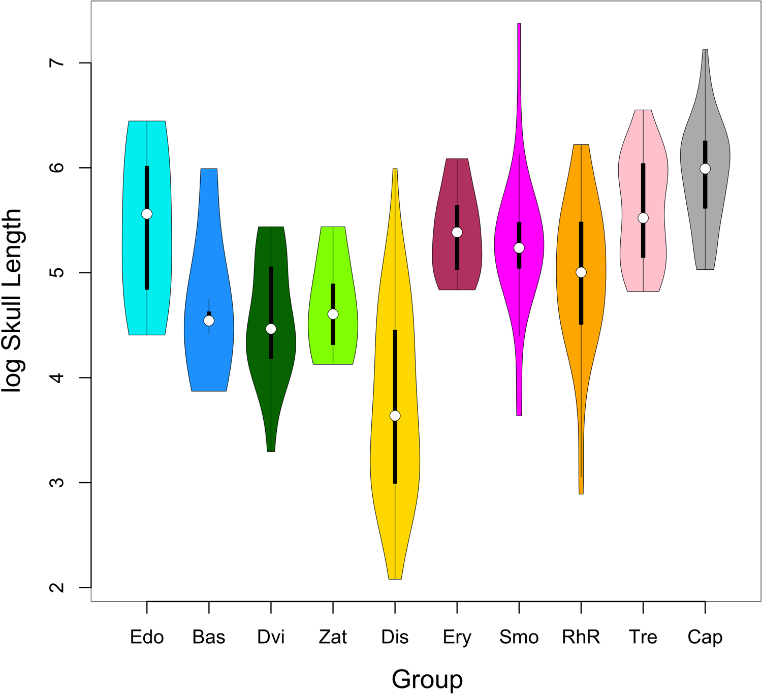
To visualise the distribution of skull lengths across taxonomic groups and time intervals, we built colour-coded violin plots in vioplot (Adler & Kelly Reference Adler and Kelly2021). For group-specific distributions of skull lengths, species were assigned to ten groups, as follows: Edopoidea (Edo; n = 7); Basal taxa (Bas; n = 5; an informal assemblage consisting of a small number of species usually placed as plesiomorphic sister taxa to distinct temnospondyl clades, e.g., species in the genera Balanerpeton, Capetus, Dendrerpeton, and Dendrysekos; Sequeira & Milner Reference Sequeira and Milner1993; Milner & Sequeira Reference Milner, Sequeira, Rolfe, Clarkson and Panchen1994; Milner Reference Milner, Milner and R.1996; Holmes et al. Reference Holmes, Carroll and Reisz1998; Schoch Reference Schoch2013b; Schoch & Milner Reference Schoch and Milner2014; Arbez et al. Reference Arbez, Atkins and Maddin2022); Dvinosauria (Dvi; n = 16); Zatracheidae (Zat; n = 5); Dissorophoidea (Dis; n= 80); Eryopidae (Ery; n = 12); Stem-Stereospondyli sensu Schoch & Milner Reference Schoch and Milner2000, broadly co-extensive with basal Stereospondylomorpha sensu Yates & Warren Reference Yates and Warren2000 (Smo; n = 28; a grade group); Rhinesuchidae + Rhytidostea (RhR; n = 49; a grade group); Trematosauroidea (Tre; n = 35); and Capitosauroidea (Cap; n = 49). Taxonomic assignments follow Schoch & Milner (Reference Schoch and Milner2000, Reference Schoch and Milner2014) and Schoch (Reference Schoch2013b). For temporal distributions of skull lengths, we assigned species to three intervals: Carboniferous; Permian; Mesozoic.
We used Kruskal–Wallis tests (‘kruskal.test’ function in base R) to assess the significance of differences in median skull length values between groups and across intervals (supplementary Table 4). In each case, we checked the significance of individual pair-wise comparisons with the ‘pairwise.wilcox.test’ function in base R, adjusting the p-values with the Benjamini & Hochberg (Reference Benjamini and Hochberg1995) correction for multiple comparisons. We also carried out phylogeny-based tests of skull length differences by performing simulation-based phylogenetic analyses of variance (Garland et al. Reference Garland, Dickerman, Janis and Jones1993) (‘phylANOVA’ function in phytools). For both groups and intervals, we carried out 1,000 simulations of the F-statistic on the phylogeny under a scenario in which groups and intervals have no effect on the distribution of trait values.
1.7. Regime shifts
To uncover regime shifts, we fitted a multi-optima OU model of skull size evolution in bayou (Uyeda & Harmon Reference Uyeda and Harmon2014). We used default values to set priors for the distributions of the OU parameters in the ‘make.prior’ function (see tutorials at: https://github.com/uyedaj/bayou/blob/master/tutorial.md) (supplementary Table 5). Such parameters include: α, the strength of the stabilising selection, which ‘attracts’ a continuous trait towards an optimum value and away from the initial value at the root of a time-calibrated phylogeny; σ 2, the variance of the trait, or rate at which trait values accrue in proportion to elapsed time; and θ, the selective optimum value for the trait (Hansen Reference Hansen1997; Butler & King Reference Butler and King2004). We imposed a maximum number of ten clade-wide regime shifts and a minimum of three shifts expected across the phylogeny. We set the prior probability for skull length values at 1.5 times the standard deviation of the measured skull lengths (e.g., see Griffin & Angielczyk Reference Griffin and Angielczyk2019). We ran the reversible-jump, Markov Chain Monte Carlo function ‘bayou.makeMCMC’ for 3 × 10⁶ generations, setting the burn-in parameter at 0.3. We visualised colour-coded regimes and their associated shifts with the ‘plotSimmap.mcmc’ function and provided a graphic representation of the Bayesian posterior probabilities (p.p.) of such shifts (at a cutoff p.p. value of 0.1) in the form of grey pie charts, the diameter of which is proportional to the p.p. of a shift.
1.8. Mean relative subclade disparity through time
To quantify the contributions of individual subclades to total skull length variation at each branching point of the supertree, we measured the mean relative subclade disparity through time (dtt; Harmon et al. Reference Harmon, Schulte, Larson and Losos2003; Murrell Reference Murrell2018) with the ‘dtt.dispRity’ function in dispRity (Guillerme Reference Guillerme2018), using the average squared Euclidean distance between taxa as a disparity index. The observed dtt curve was compared to the median dtt built from 1,000 randomly generated dtt curves under BM. We tested for significant differences between the observed dtt and the simulation-based median dtt using the morphological disparity index (MDI) statistic. MDI represents the area between the observed dtt curve and the simulated median dtt curve. If the observed dtt occurs below the simulated median dtt (MDI < 0) at a given time, then the individual subclades tend to differ from one another more than expected from random during that time (i.e., those subclades show little or no overlap across the range of skull length variation). In contrast, if the observed dtt occurs above the simulated median dtt (MDI > 0), then subclades resemble one another more than expected, i.e., they tend to overlap across the range of skull length variation. In addition, we built 50 % and 95 % confidence envelopes from the 1,000 simulated dtt curves. If the observed dtt falls outside the 95 % confidence envelope, then it is significantly different from random.
1.9. Skull length and group diversification
To establish whether changes in skull dimensions correlate with cladogenetic events, we undertook two phylogenetic generalised least squares (PGLS) regression analyses (Grafen Reference Grafen1989; Mundry Reference Mundry and Garamszegi2014; Symonds & Blomberg Reference Symonds, Blomberg and Garamszegi2014) based on the methods described by Freckleton et al. (Reference Freckleton, Phillimore and Pagel2008). In the first PGLS analysis, we regressed the trait values at the tips of the supertree (response variable) against the number of nodes separating each tip from the root of the supertree (predictor variable). In the second PGLS analysis, the number of nodes was replaced by a measure of net speciation (i.e., the rate of cladogenesis), expressed as the ratio between the number of nodes and the total temporal durations (in millions of years) of the branches separating each species from the root (supplementary Table 6). In each case, the node numbers were natural log-transformed prior to performing the PGLS analyses. The node numbers and the sums of branch durations were obtained with the ‘distRoot’ function in adephylo (Jombart & Dray Reference Jombart and Dray2010).
To perform the PGLS analyses, we employed ape and nlme (Pinheiro et al. Reference Pinheiro, Bates, DebRoy and Sarkar2021). We imposed a general correlation structure on the variance-covariance matrix built from the time-calibrated supertree, which was kept fixed throughout the duration of the parameter optimisation. As the supertree is non-ultrametric, we introduced weights, namely a fixed variance function structure applied to the diagonal values of the variance-covariance matrix (i.e., the tip-to-root lengths). After each PGLS analysis, we ran model diagnostics in the form of a quantile-quantile plot (to check for normality of residuals) and a plot of residuals versus fitted values (to check for equality of variance among residuals) (Mundry Reference Mundry and Garamszegi2014; Symonds & Blomberg Reference Symonds, Blomberg and Garamszegi2014; Witzmann & Ruta Reference Witzmann, Ruta, Ruta, Ahlberg and Smithson2019).
1.10. Temporal trends in phenotypic values and evolutionary rates
To search for temporal trends in skull length evolution, we applied a ridge regression analysis (see Kratsch & McHardy Reference Kratsch and McHardy2014; Castiglione et al. Reference Castiglione, Tesone, Piccolo, Melchionna, Mondanaro, Serio, Di Febbraro and Raia2018, Reference Castiglione, Serio, Mondanaro, Di Febbraro, Profico, Girardi and Raia2019, Reference Castiglione, Serio, Mondanaro, Melchionna, Carotenuto, Di Febbraro, Profico, Tamagnini and Raia2020) using the ‘search.trend’ function in RRphylo (Castiglione et al. Reference Castiglione, Serio, Mondanaro, Di Febbraro, Profico, Girardi and Raia2019). We applied this analysis to trait values and to evolutionary rates. For trait values, we tested for the significance of the regression of skull length values at the tips and internal nodes of the supertree against the tip and node ages (phenotypic trend test; PTT). For evolutionary rates, the branch-specific evolutionary rates were rescaled to a 0–1 range, log-transformed, and regressed against the node ages (rescaled rate trend test; RRTT) (https://cran.r-project.org/web/packages/RRphylo/vignettes/). The ridge regression method considers changes in a trait's value between a tip and an internal node as resulting from the added changes along the branches intervening between the tip and the node. Along each individual branch, the change in trait value is given by the product of the branch length multiplied by the branch rate (regression coefficient) (Kratsch & McHardy Reference Kratsch and McHardy2014; Castiglione et al. Reference Castiglione, Tesone, Piccolo, Melchionna, Mondanaro, Serio, Di Febbraro and Raia2018, Reference Castiglione, Serio, Mondanaro, Di Febbraro, Profico, Girardi and Raia2019, Reference Castiglione, Serio, Mondanaro, Melchionna, Carotenuto, Di Febbraro, Profico, Tamagnini and Raia2020).
For both PTT and RRTT analyses, we calculated the significance of the observed regression slope (p.real) and compared it to the slopes generated from 100 simulated regressions under BM (p.random). The extent to which the PTT rates deviate from BM was quantified through a deviation index. Deviation equals 0 under BM and is measured as the departure of the phenotypic mean from the trait value at the root of the phylogeny in the presence of a trend. Such departure represents the number of standard deviations of the observed trait distribution relative to BM-generated distributions (Castiglione et al. Reference Castiglione, Serio, Mondanaro, Di Febbraro, Profico, Girardi and Raia2019). The extent to which the RRTT rates deviate from BM was quantified through a spread index. Spread equals 1 under BM and is measured as the ratio of two quantities, as follows: (i) the range of observed trait values at the tips of the phylogeny divided by the range of trait values halfway along the tree height; and (ii) the same metric in (i) but with values generated under BM (Castiglione et al. Reference Castiglione, Serio, Mondanaro, Di Febbraro, Profico, Girardi and Raia2019) (supplementary Table 7).
In addition to the PTT and RRTT analyses applied to the whole tree, we investigated whether major temnospondyl groups revealed significant differences in temporal trends – both for phenotypic means and for absolute rates – relative to the rest of the tree. For these clade-wise analyses, we focused on the more speciose groups and their constituent subclades. In the case of stereospondylomorphs, we examined the entire clade (i.e., basal as well as derived groups; Schoch & Milner Reference Schoch and Milner2000) and a more restricted clade consisting of rhinesuchids, rhytidosteans, and derived stereospondyls (i.e., trematosauroids and capitosauroids). In the case of dissorophoids, we examined each of the three major lineages within this group – Micromelerpetidae, Olsoniformes, and Amphibamiformes (Boy Reference Boy1972; Anderson et al. Reference Anderson, Henrici, Sumida, Martens and Berman2008; Schoch & Milner Reference Schoch and Milner2014; Schoch Reference Schoch2019) (supplementary Table 7).
The analysis of clade-wise trends in absolute rates consists of five outputs, as follows: (i) the regression slope for the clade of interest (slope.node); (ii) the regression slope for the rest of the tree (slope.others); the significance level of the difference between those two regression slopes (p.slope); (iv) the difference in estimated marginal means for the regression models applied to the clade of interest and to the rest of the tree (emm.difference); and (v) the significance level of the differences in marginal means (p.emm). As for clade-wise trends in phenotypic means, the analysis outputs include: (i) the observed regression slope for the clade of interest (slope); (ii) the significance level of the difference between the observed slope and the slopes generated from simulations (p.slope); (iii) and (iv) the emm.difference and the p.emm, with identical meanings to those expounded above (https://cran.r-project.org/web/packages/RRphylo/vignettes/search.trend.html).
1.11. Analysis of skewness
To provide a partial test of driven trends, we applied Wang's (Reference Wang2001) analysis of skewness to the distribution of skull lengths in the ten taxonomic groups specified in section 1.6 (for additional explanations and a guided example of the skewness test, see Li et al. Reference Li, Brinkworth, Green, Oyston, Wills and Ruta2023). The R code for this analysis was kindly supplied by Professor Steve C. Wang (Swarthmore College, Pennsylvania) and is fully reproduced in Li et al. (Reference Li, Brinkworth, Green, Oyston, Wills and Ruta2023). We used the untransformed skull length values as these are positively skewed across the entire dataset as well as in each taxonomic group (Wang Reference Wang2001; Li et al. Reference Li, Brinkworth, Green, Oyston, Wills and Ruta2023) (supplementary Table 1), thereby facilitating interpretations of the percentage contributions of between-subgroup, within-subgroup, and heteroscedasticity-related values of skewness to the distribution of skull lengths across the entire set of species (Wang Reference Wang2001).
1.12. Shifts in evolutionary rates
We applied the ‘search.shift’ function in RRphylo (Castiglione et al. Reference Castiglione, Tesone, Piccolo, Melchionna, Mondanaro, Serio, Di Febbraro and Raia2018) to identify the location, magnitude, and direction of shifts in rates of trait change. To search for shifts, the function identifies all sets of taxa that include as few as 10 % and as many as 50 % of the total number of species included in the phylogeny. It then calculates the difference in mean rate value between each of those sets and the rest of the tree. The significance of each calculated difference is assessed against the differences obtained after randomly reassigning rates to the tree branches multiple times. A shift in evolutionary rate is detected when the actual rate difference is significantly lower (downturn) or higher (upturn) than expected by chance. When shifts occur at inter-nested nodes, ‘search.shift’ will select the node with the largest difference in absolute rate from the rest of the tree (Castiglione et al. Reference Castiglione, Tesone, Piccolo, Melchionna, Mondanaro, Serio, Di Febbraro and Raia2018; https://cran.r-project.org/web/packages/RRphylo/vignettes/search.shift.html). In addition, for each node where a shift is detected, the function quantifies such shift as the difference between the mean rate of the clade descending from that node (calculated as the average rate over all the clade branches) and the mean rate in the rest of the tree (Castiglione et al. Reference Castiglione, Tesone, Piccolo, Melchionna, Mondanaro, Serio, Di Febbraro and Raia2018) (supplementary Table 8).
2. Results
2.1. Timing of major cladogenetic events
The topology of the time-calibrated supertree (Fig. 1; supplementary Fig. 1; see also supplementary material for R-readable format) indicates that the phylogenetic separation between edopoids and all other temnospondyls (Eutemnospondyli sensu Schoch Reference Schoch2013b) occurred close to the Tournaisian–Viséan boundary, implying that a substantial portion of the early diversification of edopoids must have taken place during the Mississippian and early Pennsylvanian (see also discussion in Milner & Sequeira Reference Milner and Sequeira1998). This estimated divergence time is consistent with the occurrence of possible edopoid fragments in the Viséan site of East Kirkton, Scotland, which has also produced abundant and well-preserved specimens of the putative basal temnospondyl Balanerpeton woodi (Milner & Sequeira Reference Milner, Sequeira, Rolfe, Clarkson and Panchen1994). Within eutemnospondyls is a dichotomy between a group inclusive of dvinosaurs, zatracheids, and dissorophoids and a group – termed the Eryopiformes (Schoch Reference Schoch2013b; corresponding to the Eryopoidea sensu Boy Reference Boy1988) – that encompasses eryopids and stereospondylomorphs. These two groups (Rhachitomi sensu Schoch Reference Schoch2013b) are estimated to have diverged in the mid Viséan, and the initial diversification of each was well underway by the mid Serpukhovian. By this same time interval, dvinosaurs had separated from the zatracheid-dissorophoid clade, while the three main lineages of dissorophoids – Micromelerpetidae, Olsoniformes, and Amphibamiformes – had appeared by the early Moscovian. The diversification of basal stereospondylomorphs spanned the Kasimovian to Capitanian time interval, while derived stereospondyls are likely to have emerged in the late Permian. Lastly, the separation between trematosauroids and capitosauroids is minimally dated to the early-middle part of the Wuchiapingian.
Time-calibrated supertree of temnospondyls plotted against geologic time. Time (in millions of years) is represented by the graduated scale. Reconstructed skulls of representative species are shown. The thick, black rectangular bars at the end of the terminal branches indicate the stratigraphic ranges of taxa, from first to last appearance datum. To avoid label crowding, taxon names have been omitted (see supplementary Fig. 1). The figured skulls (right to left, not drawn to scale) belong to: the edopoid Edops craigi (redrawn after Romer & Witter Reference Romer and Witter1942); the dissorophoids Cacops morrisi (redrawn after Reisz et al. Reference Reisz, Schoch and Anderson2009) and Apateon pedestris (redrawn after Schoch & Milner Reference Schoch and Milner2008); the eryopid Eryops megacephalus (redrawn after Sawin Reference Sawin1941); the rhytidostean Eolydekkerina magna (redrawn after Shishkin et al. Reference Shishkin, Rubidge and Kitching1996); the trematosauroid Anaschisma browni (redrawn after Gee & Jasinski Reference Gee and Jasinski2021); the capitosauroid Mastodonsaurus giganteus (redrawn after Schoch Reference Schoch1999).

2.2. Strength of phylogenetic signal and comparisons between evolutionary models
The distribution of skull length values across species is strongly influenced by phylogeny (Pagel's λ = 0.924038; log-likelihood (λ) = −265.683). The fitted value of λ is significantly different from 0 (p-value = 8.90798 × 10−79) but not from 1 (p-value = 1). Furthermore, the variance of skull lengths is mostly partitioned within, rather than among, groups, as indicated by the low value of Blomberg's K (0.246768; p-value = 0.001). The observed Moran's I (0.2885264) is positive and significantly (p-value << 0.05) higher than the value expected under BM (−0.003484321), indicating a strong positive autocorrelation (i.e., trait values in closely related species resemble each other more than expected).
The best-fitting model of continuous trait evolution is kappa, or punctuated evolution (supplementary Table 2), and this is significantly better than the second best-fitting model lambda (likelihood-ratio test: LR = 32.89787; p-value = 0). The very low value of the kappa parameter (k = 0.197234; AICc = 504.553301; log-likelihood = −249.234397) would seem to indicate that changes in skull size were mainly concentrated near speciation events, with longer branches characterised by greater than expected stasis and shorter branches exhibiting greater than expected change (Pagel Reference Pagel1999). However, we present a cautionary note on these results. The difference in trait values between any two species depends on the number of branching events that intervene between those species. It follows that the kappa model is heavily influenced by extinctions and missing portions of the phylogeny, such as those due to incomplete taxon sampling (Pagel Reference Pagel1999; Pennell et al. Reference Pennell, Harmon and Uyeda2014b). Pending a more in-depth scrutiny of models of phenotypic diversification and an assessment of the quality of the temnospondyl record, the prevalence of the kappa model should only be regarded as provisional.
The node height test (supplementary Fig. 2) indicates a weak positive relationship between the natural log-transformed absolute values of the independent contrasts at the internal nodes of the phylogeny and the distance of the nodes from the root. This result implies that the differences in skull length between species tend to increase towards less deep (i.e., more recent) nodes of the phylogeny. Both the slope (0.0051) and the intercept (−2.6147) of the robust linear regression model differ significantly from zero (slope: F = 4.9135; p-value = 0.02744; intercept: F = 240.64; p-value = 2.2 × 10⁻¹⁶). In conjunction with the model fitting analyses presented above, these results allow us to reject EB as a viable model of skull length evolution in temnospondyls.
2.3. Changes in skull length across phylogeny
Colour-coded changes in skull length mapped onto the supertree (Fig. 2) reveal complex patterns of trait variation. A remarkable diversity of skull sizes is documented throughout the Carboniferous and first half of the Permian, with skulls ranging from diminutive (e.g., in several dissorophoids) to very large (e.g., in some edopoids, eryopids, and basal stereospondylomorphs). From the middle Permian through to the end of the Mesozoic (and particularly in the Triassic), species exhibiting mid-sized to extremely large skulls are increasingly common, especially among basal stereospondylomorphs (e.g., 1,600 mm in Prionosuchus plummeri; Cox & Hutchinson Reference Cox and Hutchinson1991) as well as in trematosauroids (e.g., 700 mm in Benthosuchus sushkini; Schoch & Milner Reference Schoch and Milner2000) and capitosauroids (e.g., 1,250 mm in Mastodonsaurus giganteus; Schoch & Milner Reference Schoch and Milner2000). Examples of taxa with very small skulls are also documented in this time interval, including the dvinosaur Thabanchuia oomie (27 mm; Warren Reference Warren1998), the dissorophoids Tungussogyrinus bergi (11 mm; Werneburg Reference Werneburg2009) and Micropholis stowi (37 mm in short-skulled morphs; Schoch & Rubidge Reference Schoch and Rubidge2005), and the basal stereospondyls Lapillopsis nana (23 mm; Warren & Hutchinson Reference Warren and Hutchinson1990) and Nanolania anatopretia (18 mm; Yates Reference Yates2000).
Colour-coded values of natural log-transformed skull lengths mapped onto a time-calibrated supertree of temnospondyls. The colours at the tips of the terminal branches refer to the trait values of the individual taxa; the colours at the internal nodes represent maximum likelihood ancestral estimates of trait values; the colour gradients along the branches result from value interpolations (see text for explanations). The minimum and maximum trait values are reported at the extremities of the colour scale bar. The black arrows point to the latest common nodes of major temnospondyl groups. Abbreviations: Edo = Edopoidea; Bas = Basal taxa; Dvi = Dvinosauria; Zat = Zatracheidae; Dis = Dissorophoidea; Ery = Eryopidae; Smo = Stem-Stereospondyli; RhR = Rhinesuchidae + Rhytidostea; Tre = Trematosauroidea; Cap = Capitosauroidea.

Ancestral trait estimates suggest that the common ancestor of temnospondyls had a skull length slightly exceeding 120 mm (supplementary Table 3). Near the base of the temnospondyl radiation, a decrease in skull length is documented at the nodes that subtend the edopoid-eutemnospondyl divergence (>115 mm) and the origin of the rhachitomes (>99 mm). Distinctly longer skulls are estimated for the common ancestors of edopoids (>141 mm), eryopids (>160 mm), derived stereospondylomorphs (>236 mm), rhinesuchids (>258 mm), rhytidosteans (>127 mm), capitosauroids (>190 mm), and trematosauroids (>200 mm). In contrast, mid-sized to small skulls are estimated to have been present in the common ancestors of zatracheids (>88 mm), dvinosaurs (>87 mm), and dissorophoids (>45 mm) (Figs 1, 2; supplementary Fig. 1 and Table 3).
One of the most interesting patterns of skull size changes relates to the Xerodromes (Schoch & Milner Reference Schoch and Milner2014); that is, all dissorophoids more derived than Micromelerpetidae. Xerodromes comprise two major groups, the Olsoniformes (Anderson et al. Reference Anderson, Henrici, Sumida, Martens and Berman2008) and the Amphibamiformes (Schoch Reference Schoch2019). For both groups, and with reference to the ‘right-ladderized’ supertree topology, we recorded skull length estimates at the progressively less inclusive nodes that make up the ‘backbone’ of their respective phylogenies (Fig. 1; supplementary Fig. 1 and Table 3). The backbone phylogeny of olsoniforms consists of nodes 505 to 517, where 505 is the most inclusive node subtending all taxa between Palodromeus bairdi (Schoch et al. Reference Schoch, Henrici and Hook2021) and Parioxys ferricolus (Schoch & Sues Reference Schoch and Sues2022) and 517 is the least inclusive node leading to Kamacops acervalis (Gubin Reference Gubin1980) and Parioxys ferricolus. Estimated skull lengths increase slowly from node 505 to node 510. A negligible decrease from node 510 to node 512 is followed by a second, steep increase from node 512 to node 517. To sum up, from the most inclusive to the least inclusive node of their backbone phylogeny, olsoniforms show an overall skull length increase of ~268 % (supplementary Table 3).
The backbone phylogeny of amphibamiforms comprises nodes 472 to 483, where 472 is the most inclusive node subtending all taxa between Tersomius dolesensis (Anderson & Bolt Reference Anderson and Bolt2013) and Apateon caducus (Fröbisch & Schoch Reference Fröbisch and Schoch2009) and 483 is the least inclusive node leading to Apateon flagrifer (Werneburg Reference Werneburg1989) and Apateon caducus. Changes in estimated skull lengths along these nodes reveal a more elaborate pattern than those in olsoniforms, with a rapid initial decrease from node 472 to node 477, a small increase from node 477 to node 478, a second sharp decrease from node 478 to node 480, and a novel steep increase from node 480 to node 483. From the most inclusive to the least inclusive node of their backbone phylogeny, amphibamiforms show an overall skull length reduction of ~40 % (supplementary Table 3).
In other domains of temnospondyl phylogeny, similarly elaborate patterns are observed. We mention briefly those related to capitosauroids and trematosauroids. In the backbone phylogeny of capitosauroids, from node 307 to node 325 (where 307 is the most inclusive node subtending all taxa between Wetlugasaurus angustifrons (Riabinin Reference Riabinin1930) and Cyclotosaurus naraserluki (Marzola et al. Reference Marzola, Mateus, Shubin and Clemmensen2017) and 325 is the least inclusive node subtending all taxa between Cyclotosaurus mordax (Fraas Reference Fraas1913) and Cyclotosaurus naraserluki), skull length increased by ~115 %, despite a substantial drop across nodes 315–318 (supplementary Table 3). As for trematosauroids, reconstructed ancestral estimates indicate an overall drop in skull length by ~18 %, from node 355 (the most inclusive node subtending all taxa between Edingerella madagascariensis (Lehman Reference Lehman1961) and Microposaurus casei (Haughton Reference Haughton1925)) to node 366 (the most inclusive node subtending all taxa between Platystega depressa (Wiman Reference Wiman1914) and Microposaurus casei) of their backbone phylogeny. However, this decrease is not linear and reveals alternating increases and decreases (supplementary Table 3). Among post-benthosuchid trematosauroids, the almasaurid-metoposaurid clade shows a strikingly contrasting pattern, with a linear and steady increase in skull lengths by about 45 %.
2.4. Mean skull length differences between taxonomic groups and time intervals
Kruskal–Wallis tests show significant differences in skull lengths across taxonomic groups (Fig. 3; chi-squared = 168.74; df = 9; p-value <2.21 × 10⁻¹⁶) and time intervals (supplementary Fig. 3; chi-squared = 64.88; df = 29; p-value = 8.155 × 10⁻¹⁵). Out of 45 pair-wise comparisons between groups, 24 are significant and four are marginally non-significant. In contrast, all three pair-wise comparisons between intervals are significant, with median skull length increasing from Carboniferous to Permian and from Permian to Mesozoic (supplementary Table 4).
Violin plots illustrating the distribution of natural log-transformed skull lengths colour-coded by taxonomic group (see text for group delimitations). Each violin shows the probability density distribution of trait values (violin contours), the median value (white circle), and the interquartile range (thick black vertical bar). Abbreviations: Edo = Edopoidea; Bas = Basal taxa; Dvi = Dvinosauria; Zat = Zatracheidae; Dis = Dissorophoidea; Ery = Eryopidae; Smo = Stem-Stereospondyli; RhR = Rhinesuchidae + Rhytidostea; Tre = Trematosauroidea; Cap = Capitosauroidea.

Unlike the Kruskal–Wallis tests, however, phylogenetic analyses of variance return no significant results for groups and intervals. One possible explanation for this discrepancy is that a phylogenetic analysis of variance seeks to establish whether similar trait values between species are ‘conditioned’ by the grouping variable (i.e., taxonomic groups; time intervals) or whether they are due to relatedness (shared ancestry). Clustering of trait values across phylogeny often results in higher p-values than in the case of standard (i.e., non-phylogenetic) comparisons (see exchange at: https://r-sig-phylo.r-project.narkive.com/BQN6doRK/help-interpreting-phylogenetic-anova-results). Indeed, as shown above, measures of phylogenetic autocorrelation strongly indicate that skull dimensions in phylogenetically proximal species tend to be more similar than expected.
2.5. Distribution of regime shifts
The multi-optima model fitting analysis in bayou retrieves ten regime shifts at the 0.1 cutoff value for posterior probabilities (p.p.) (Fig. 4; supplementary Table 5). Several shifts occur along the early-diverging branches of various major clades and are invariably associated with low or moderate p.p. The most conspicuous shift, with a p.p. of 0.448, is located along the branch that subtends (Trematosauroidea + Capitosauroidea) (node 306). The second, third, and fourth largest shifts occur along the branches that subtend the following clades, respectively: (Dvinosauria + (Zatracheidae + Dissorophoidea)) (node 465; p.p. = 0.334); (Dendrerpeton confusum + Dissorophoidea) (node 467; p.p. = 0.33), with Perryella olsoni (Ruta & Bolt Reference Ruta and Bolt2006) and Macrerpeton huxleyi (Schoch & Milner Reference Schoch and Milner2021) forming the two most basal taxa within dissorophoids; Olsoniformes (node 505; p.p. = 0.322). In descending order of p.p. values, four additional shifts are recovered in Dissorophoidea inclusive of Perryella olsoni and Macrerpeton huxleyi (node 468; p.p. = 0.292), Olsoniformes exclusive of Palodromeus bairdi (node 506; p.p. = 0.259), Amphibamiformes (node 472; p.p. = 0.257), and Micromelerpetidae (node 536; p.p. = 0.243). Lastly, two negligible shifts characterise the branches that subtend (Dendrerpetidae + (Dvinosauria + (Zatracheidae + Dissorophoidea))) (node 464; p.p. = 0.202) and Olsoniformes exclusive of Palodromeus bairdi and Actiobates peabodyi (Gee & Reisz Reference Gee and Reisz2020) (node 507; p.p. = 0.12). Numerous additional shifts, represented by minuscule circles of varying sizes in Fig. 4, are dotted around other major groups of temnospondyls, but they all fall under the 0.1 cutoff value for posterior probabilities and do not require additional comments.
Time-calibrated supertree of temnospondyls with regimes mapped in different colours on the tree branches and with regime shifts indicated by grey circles. The size of the circles is proportional to the posterior Bayesian probability of the shifts. For reference, the largest posterior probability, plotted at the node subtending the radiation of Trematosauroidea + Capitosauroidea, equals 0.4481535 (see text for the identity of nodes featuring shifts). The colour-coded rectangular panels delimit major temnospondyl groups. Abbreviations: Edo = Edopoidea; Bas = Basal taxa; Dvi = Dvinosauria; Zat = Zatracheidae; Dis = Dissorophoidea; Ery = Eryopidae; Smo = Stem-Stereospondyli; RhR = Rhinesuchidae + Rhytidostea; Tre = Trematosauroidea; Cap = Capitosauroidea.

2.6. Partition of skull length variation across subclades
In the analysis of mean relative subclade disparity through time, the observed dtt curve occurs below the median curve generated from simulated dtt values (MDI = −0.1557495) but falls mostly within the 95 % confidence envelop (p-value = 0.907), indicating that it does not depart significantly from random. This pattern dominates throughout the Palaeozoic, during large time intervals within the Triassic (except as noted below), and among post-Triassic groups (Fig. 5).
Plot of mean relative subclade disparity through time (dtt), using the average squared Euclidean distance between taxa as a disparity index. The thick, solid black line is the observed dtt. The thin, dashed black line is the median dtt obtained from 1,000 randomly simulated dtt curves under a Brownian motion process of evolution. The grey areas represent the confidence envelopes built from the 1,000 simulations, using 50 (light grey) and 95 (dark grey) quantiles. Scaled relative time (on the horizontal axis) corresponds to the depth of the supertree (i.e., the temporal duration from the age of the root to the age of the youngest species) and is subdivided into regularly spaced intervals.

There are two short time intervals during which the observed dtt plots out above the simulated median dtt. The first interval coincides approximately with the middle one-third of the Norian (Upper Triassic). Here, the observed dtt occurs mostly within the boundaries of the 50 % confidence envelope, except for a conspicuous ‘spike’ in the middle part of the Norian that falls outside the 95 % confidence envelope. The second interval is approximately co-extensive with the Ladinian (Middle Triassic), with the observed dtt similarly occurring within the 50 % confidence envelope.
Changes in dtt follow distinct patterns throughout temnospondyl history. A steady decrease is observed throughout the Carboniferous and up to the Sakmarian (lower Cisuralian). This decrease is steep and uniform from the Tournaisian to the early Serpukhovian, less conspicuous and with irregular fluctuations up to the Gzhelian, then markedly steep again throughout the Asselian and Sakmarian. Alternating increases and decreases of varying magnitude are observed throughout the rest of the Permian, with an overall tendency for dtt to rise imperceptibly. A marked drop in the Lower Triassic is followed by a rapid increase throughout the Middle Triassic. The most complex changes are observed in the Upper Triassic. An initial, slow drop in dtt throughout the Carnian is followed by four spikes of increasing magnitude during the first part of the Norian, with the fourth and largest spike as described above. After this time, dtt shows irregular fluctuations in the form of unremarkable increases and decreases during the Rhaetian. In the earliest part of the Jurassic, dtt rebounds to levels that are only slightly lower than those documented in the latest Triassic. Further small fluctuations are observed throughout the Sinemurian. After this time, dtt decreases steadily throughout the terminal part of the Mesozoic history of temnospondyls (Fig. 5).
2.7. Phenotypic changes and group diversification
Figures 6 and 7 show bivariate scatterplots of trait values at the tips of the supertree versus two indices of group diversification, namely the number of nodes separating taxa from the tree root and the net speciation rate. Each scatterplot features the trend line deriving from a PGLS regression of trait values versus index. In neither case is the slope of the relationship significant, although the intercept differs significantly from zero in both analyses (see supplementary Table 6 for PGLS model diagnostics). Despite the lack of significance in the slopes, it is instructive to note that the tip values correlate positively, albeit very weakly, with the number of nodes separating the taxa from the root of the tree (Fig. 6). This result is in broad agreement with that of the node height test: in both cases, greater trait divergence is correlated with larger numbers of root-to-tip branching events (see also the PTT below). However, when the root-to-tip distances are corrected by the amount of elapsed time, a weak negative correlation occurs between tip values and net speciation (Fig. 7), suggesting that increases in rates of cladogenesis (the number of branching events per unit time) tend to be primarily associated with the evolution of small-sized taxa.
Bivariate scatterplot of natural log-transformed skull lengths versus natural log-transformed number of nodes separating each species from the root of the supertree, based upon a phylogenetic generalised least squares regression. The regression line is shown in blue. Species are colour-coded by taxonomic group.

Bivariate scatterplot of natural log-transformed skull lengths versus cladogenetic rate, based upon a phylogenetic generalised least squares regression. The cladogenetic (or diversification) rate is calculated as the ratio between the natural log-transformed number of nodes separating each species from the root of the supertree and the summed temporal durations of the intervening branches. The regression line is shown in blue. Species are colour-coded by taxonomic group.

2.8. Temporal trends in skull length evolution
Changes in skull size and evolutionary rates through time reveal substantial heterogeneities across groups. Figure 8 shows bivariate scatterplots and associated regression slopes for phenotypic values (i.e., skull lengths) at the tips/nodes of the phylogeny versus tip/node ages (PTT; left panel) and for branch-specific evolutionary rates versus node ages (RRTT; right panel). The results of ridge regression analyses for individual groups are reported in supplementary Table 7, supplementary material, and extended data Figs 1–12 (see Discussion).
Bivariate scatterplots generated from ridge regression analyses of temporal trends for phenotypes (left panel) and evolutionary rates (right panel) regressed against time. In each scatterplot, the red and green circles represent values (phenotypes at left; rates at right) at the tips and nodes of the phylogeny, respectively. The grey areas are 95 % confidence envelopes of slopes built from 100 simulated regressions under BM. The blue line is the observed regression line. Relative time (on the horizontal axis) corresponds to the depth of the supertree in millions of years (more recent times towards the right of the axis).

The PTT and the RRTT tests applied to the entire tree (Fig. 8; supplementary Table 7) indicate that both phenotypic values (p.real = 2.584661 × 10−56) and evolutionary rates (p.real = 5.472011 × 10⁻⁵) correlate positively and significantly with ages. In the case of PTT, contrasting the observed regression slope with randomly generated BM slopes reveals an actual temporal trend (p.random = 1; dev = 2.300972). Specifically, the results depart significantly from BM by more than twice the standard deviation of the trait mean from the value at the root. In the case of RRTT, however, the absolute increase in evolutionary rates over time does not depart significantly from BM (p.random = 0.27), and the observed increase in rate over time is only marginally higher (spread = 1.000108) than the rate that would be expected under a null model.
Across individual groups, changes in phenotypic means and evolutionary rates through time reveal contrasting patterns (supplementary Table 7, supplementary material, and extended data Figs 1–12). Trends in phenotypic mean are positive and significantly higher than BM simulations in edopoids and olsoniforms (extended data Figs 1, 5), positive and marginally non-significant in dissorophoids and trematosauroids (extended data Figs 3, 10), and positive but non-significant in most other groups (eryopids are the sole exception, in that they show a negative, albeit non-significant phenotypic slope). Estimated marginal means associated with the regressions of phenotypes versus node ages are significantly larger than in the rest of the tree in edopoids, eryopids, stereospondylomorphs, the rhinesuchid-rhytidostean-derived stereospondyl clade, and capitosauroids. Estimated marginal means that are significantly lower than in the rest of the tree are documented in dissorophoids as a whole and, among them, in micromelerpetids, and amphibamiforms (supplementary Table 7).
Concerning trends in evolutionary rates, edopoids, dvinosaurs, zatracheids, eryopids, and stereospondylomorphs show positive but non-significant regression slopes. Of the remaining groups – all with negative slopes – only trematosauroids and capitosauroids show a significant decrease in rates through time (extended data Figs 10, 11). Estimated marginal means are significantly larger than in the rest of the tree in three groups: stereospondylomorphs; rhinesuchids-rhytidosteans-derived stereospondyls; and trematosauroids (supplementary Table 7).
2.9. Analysis of skewness
Wang's (Reference Wang2001) analysis of skewness shows that within-group skewness accounts for nearly two-thirds (62.6 %) of the total skewness in skull length values across the entire dataset. The heteroscedasticity-related component of skewness is less conspicuous (33.3 %), and the between-group component is very small (4.1 %). These results appear to be consistent with a driven trend (McShea Reference McShea1994; Wang Reference Wang2001) – i.e., the evolution of skull length can be characterised as a sustained tendency, with changes occurring in parallel in separate groups. The results of the skewness test, however, also demonstrate that passive processes exerted a non-negligible influence on skull length evolution, a frequent outcome in these types of analyses (Wang Reference Wang2001; Li et al. Reference Li, Brinkworth, Green, Oyston, Wills and Ruta2023). This result may be explained by noting that there are differences in skewness across individual groups, as reflected by the contribution of the heteroscedasticity component. Thus, whereas the untransformed skull lengths are positively skewed in all groups, their distribution is very slightly asymmetrical in some of them (e.g., trematosauroids; edopoids; dvinosaurs) but markedly asymmetrical in others (e.g., basal stereospondylomorphs; dissorophoids) (supplementary Table 1), pointing to varying degrees of trait value dispersal among species and the influence of outlying taxa, i.e., species displaying unusually large or small skulls.
2.10. Tree-wise rate shifts
The two nodes with the largest significant shifts in evolutionary rates are mapped onto the supertree in Fig. 9. The first shift, a rate downturn at node 464 (blue circle), subtends dendrerpetids, dvinosaurs, zatracheids, and dissorophoids. The rate difference between node 464 and the rest of the tree (−0.06872578) is significantly smaller than expected by chance. The second shift, a rate upturn at node 357 (maroon circle), accompanies the diversification of post-benthosuchid trematosauroids, that is, all taxa bracketed by, and including, Almasaurus habbazi and Microposaurus casei. The rate difference between node 357 and the rest of the tree (0.21275128) is significantly larger than expected by chance (supplementary Fig. 1).
Time-calibrated supertree of temnospondyls with the two most significant shifts in evolutionary rates indicated by circles. The size of the circles is proportional to the absolute value of the absolute rate difference between a node and the rest of the tree (see text for detail). The blue circle marks a rate downturn at the node subtending dendrerpetids, dvinosaurs, zatracheids, and dissorophoids. The maroon circle marks a rate upturn at the node subtending post-benthosuchid trematosauroids. The black arrows point to the latest common nodes of major temnospondyl groups. Abbreviations: Edo = Edopoidea; Bas = Basal taxa; Dvi = Dvinosauria; Zat = Zatracheidae; Dis = Dissorophoidea; Ery = Eryopidae; Smo = Stem-Stereospondyli; RhR = Rhinesuchidae + Rhytidostea; Tre = Trematosauroidea; Cap = Capitosauroidea.

Other nodes exhibiting smaller differences in average rate relative to the rest of the tree are reported in supplementary Table 8. Fifteen of those nodes are characterised by significant upturns, while another 11 feature significant downturns. Rate upturns occur along a series of 13 inter-nested nodes forming the backbone phylogeny of a diverse array of taxa that extends from the apical portion of basal stereospondylomorphs (node 300) to the sixth basalmost node along the backbone phylogeny of capitosauroids (node 312). Two additional instances of small rate upturns appear at the two basalmost nodes along the backbone phylogeny of trematosauroids (nodes 355 and 356). Rate downturns similarly characterise a series of interested nodes (465 to 471) along the backbone phylogeny of the dvinosaur-zatracheid-dissorophoid radiation. Three additional downturns appear in sequence along the three basalmost nodes forming the backbone phylogeny of olsoniforms (505 to 507). Lastly, a small downturn at node 390 accompanies the diversification of basal stereospondyls immediately more derived than the rhytidostean clade that includes lydekkerinids and lapillopsids (supplementary Fig. 1).
2.11. Phylogenetically corrected taxic diversity through time
The plot of phylogenetically corrected taxic diversity through time (extended data Fig. 13; see also Ruta & Benton Reference Ruta and Benton2008) features a series of alternating increases and decreases. The first increase is documented from the late Tournaisian or earliest Viséan to the late Asselian and includes two phases. The first phase is represented by a slow rise in taxic diversity up to the early Moscovian, possibly reflecting the sparse record of lower to early Middle Carboniferous temnospondyls (Schoch & Milner Reference Schoch and Milner2014). The second phase is marked by a steep and rapid rise in diversity up to approximately the first two-thirds of the Kasimovian. After this time, diversity drops slightly until the end of the Kasimovian and then rebounds rapidly, attaining its largest recorded value in the latest part of the Asselian. From the Asselian to the Roadian, temnospondyl diversity experiences a conspicuous decrease, also marked by two consecutive phases. The first phase is characterised by a steady decline lasting until the middle part of the Kungurian (with irregular fluctuations represented by small, alternating spikes and drops). The second phase features a distinctly sharper drop extending until the middle part of the Roadian. From then on, diversity rises again steeply, reaching a peak in the late part of the Changhsingian. The pattern of diversity changes that immediately precedes the end-Permian mass extinction consists of a slight decline close to the end-Changhsingian, followed by a small rise in the earliest part of the Induan. After this time, diversity decreases rapidly in the remaining part of the Induan and then rebounds irregularly – with alternating peaks and troughs – during the Olenekian. After this time, diversity decreases rapidly throughout the Mesozoic. The only departures from the overall trend of declining diversity in the Mesozoic are observed in two short time intervals – one, already mentioned, in the Olenekian, the other (less conspicuous) encompassing the second half of the Anisian and first half of the Ladinian – during which diversity shows inconspicuous variations.
3. Discussion
3.1. Adaptive optima
Regime shifts feature primarily as a series of inter-nested, pulse-like events concentrated along the basal branches of the dvinosaur-zatracheid-dissorophoid radiation. An additional shift occurred along the branch subtending the trematosauroid-capitosauroid divergence (Fig. 4). The distribution of the inter-nested shifts in the dvinosaur-zatracheid-dissorophoid clade matches fundamental changes in developmental patterns, ecological adaptations, and feeding modes (Schoch & Witzmann Reference Schoch and Witzmann2024), which allowed temnospondyls to colonise a broad range of terrestrial and aquatic settings and exploit new food resources, possibly as early as the early-mid part of the Mississippian. The shift along the common stem of trematosauroids and capitosauroids coincides with ubiquitous records of derived stereospondyls in water bodies of Pangea (Schoch & Milner Reference Schoch and Milner2000; Liu et al. Reference Liu, Angielczyk and Abdala2021; see below).
Inspection of Fig. 4 reveals no change in adaptive optima (i.e., no regime shifts) along the backbone phylogeny of temnospondyls. In this respect, it may also be instructive to note that there are no significant differences in mean skull lengths in any pair-wise comparisons among edopoids, eryopids, basal stereospondylomorphs, and early diverging groups from among derived stereospondyls (rhinesuchids and rhytidosteans) (supplementary Table 4). All these groups may have shared a series of developmental and morphofunctional traits that are thought to be plesiomorphic for temnospondyls, such as external larval gills, internal adult gills, and a mode of feeding that involved a unidirectional water flow through the mouth in larval stages and in aquatic or semi-aquatic adults (Schoch & Witzmann Reference Schoch and Witzmann2024). The most conspicuous changes in one or more of these characteristics affected for the most part the dvinosaur-zatracheid-dissorophoid clade, as detailed by Schoch & Witzmann (Reference Schoch and Witzmann2024).
The regime shift separating basal temnospondyls (‘dendrerpetids’) from the dvinosaur-zatracheid-dissorophoid clade coincides with the enlargement of the pectoral girdle in larvae (Schoch & Witzmann Reference Schoch and Witzmann2024), also observed within Eryopiformes. Interestingly, however, no regime shifts are found along the branches subtending dvinosaurs and zatracheids-dissorophoids (Fig. 4), despite a drastic modification in the ontogeny and lifestyles of the adults of those groups. While dvinosaurs developed elongate bodies and were fully aquatic organisms with internal gills as adults, zatracheids evolved compact, stout, and abbreviated bodies and were fully terrestrial animals that lost gills in their adult stages. In spite of their divergent ecologies and ontogenies, dvinosaurs and zatracheids do not differ significantly in mean skull length (supplementary Table 4). At least primitively, reduction and loss of internal gills characterises dissorophoids as well, with certain developmental strategies, such as neoteny, evolving ex novo in some lineages within the clade (branchiosaurids; amphibamids). Each of three major groups of dissorophoids (micromelerpetids; olsoniforms; amphibamiforms) shows a regime shift at its basalmost branch, although it is not immediately obvious how such shifts relate to developmental remodelling.
3.2. Phylogenetic partitioning
The analysis of mean relative subclade disparity through time indicates that skull length variation is almost invariably greater among than within groups (Fig. 5), since the observed dtt plots out below the median dtt generated from the BM simulations. This result could be interpreted as evidence of niche partitioning, consistent with the remarkable array of morphologies and ecologies exhibited early in the group's history. The rapid apportioning of skull length variation to diverging lineages (i.e., separation in trait space between groups), such as is demonstrated by the rapid and sustained decrease in dtt, persisted for nearly 35 million years throughout the Mississippian and Lower Pennsylvanian, by which time most major clades had appeared (Fig. 1). Disparity appears to have fluctuated irregularly around a long-term mean from the Middle Pennsylvanian to the end-Guadalupian, but it remained consistently lower than the expected simulated median, pointing to additional episodes of phenotypic differentiation, both in the later history of some groups (e.g., dvinosaurs, dissorophoids, and eryopids) and during the initial diversification of newly diversifying groups (e.g., rhinesuchids and rhytidosteans). A marked departure from this trend took place from the Lopingian to the early Upper Triassic, when the observed dtt began to increase more or less continuously, reaching a spike around the Middle Triassic. During this time interval, different temnospondyl clades convergently attained similar cranial dimensions (i.e., overlap in trait space between groups). This pattern can be accounted for by the appearance of large-sized and even gigantic forms within trematosauroids, capitosauroids, eryopids, and basal stereospondylomorphs (Figs 1, 5; extended data Fig. 14). Somewhat counterintuitively, the observed dtt decreases again in the rest of the Mesozoic, once again occurring below the level of the simulated median dtt. Lastly, two irregular rises are observed in the late part of the Upper Triassic and during the early-middle Lower Jurassic. This pattern is associated with later members of morphologically disparate groups (including possible relict forms; Milner Reference Milner, Fraser and Sues1994), such as chigutisaurids, metoposaurids, and capitosauroids, across which skull lengths range from small-medium (137 mm) to very large (625 mm).
3.3. Evolutionary trends in skull size and the lifestyles of temnospondyls
The analyses of evolutionary trends (both for phenotypic values and for rates of trait change) reveal inextricably complex patterns at different levels of taxonomic inclusiveness (Fig. 8; extended data Figs 1–12). An overarching tendency towards increases in skull size over time is supported – albeit weakly – for temnospondyls as a whole (Fig. 8, left panel; supplementary Table 7) and is likewise reflected in the temporal distribution of skull lengths (supplementary Fig. 3 and Table 4), with Mesozoic values significantly exceeding those in the Carboniferous and Permian. This trend appears to have been mainly driven by the two major radiations of derived stereospondyls – the predominantly aquatic trematosauroids and capitosauroids – but also, to a lesser degree, by individual species and clades within basal stereospondylomorphs, rhinesuchids, and rhytidosteans (Fig. 3). It is worth reiterating that, with the exception of eryopids, most other temnospondyl groups also reveal negligible to moderate increases in skull length over time. Coupled with the outcome of the skewness test, these results support the notion of directional and sustained changes (McShea Reference McShea1994; Wang Reference Wang2001). If corroborated, this finding would constitute one of the very few instances of explicitly tested driven trends documented so far, alongside previous case studies that include increase in complexity in crustacean tagmosis (Adamowicz et al. Reference Adamowicz, Purvis and Wills2008) and increase in vertebral column differentiation in mammals (Li et al. Reference Li, Brinkworth, Green, Oyston, Wills and Ruta2023).
If indeed skull size evolved according to a driven process, then it is appropriate to ask what selective advantages – if any – a size increase might have afforded. Large size may have allowed temnospondyls to escape or buffer against predation, although an unequivocal test of this hypothesis appears arduous at present. At the beginning of the Mesozoic, several temnospondyls had themselves become apex predators in predominantly freshwater bodies across various domains of Pangea, long before other tetrapods – especially archosaur diapsids – became dominant, but in completely different ecological settings (terrestrial environments) and at a slightly later time. An aquatic lifestyle is ubiquitous among temnospondyl groups such as basal stereospondylomorphs, trematosauroids, and capitosauroids, and is evidenced by sensory canals, poorly ossified postcranial skeletons, absence or reduction of processes on limb bones, pachyostosis, and internal gills in adults (Schoch & Milner Reference Schoch and Milner2000; Marsicano et al. Reference Marsicano, Latimer, Rubidge and Smith2017; Schoch & Witzmann Reference Schoch and Witzmann2024). Free from the biomechanical constraints linked to life on land, several members of these groups attained large or even gigantic dimensions and a sheer variety of ecomorphotypes – from crocodile or gharial-like hunters to bottom-dwelling ambush predators (Damiani Reference Damiani2001b; Jenkins Jr et al. Reference Jenkins, Shubin, Gatesy and Warren2008; Konietzko-Meier et al. Reference Konietzko-Meier, Gruntmejer, Marcé-Nogué, Bodzioch and Fortuny2018; Kalita et al. Reference Kalita, Teschner, Sander and Konietzko-Meier2022). In addition to providing body support, the aquatic environment also supplied temnospondyls with a rich and diverse variety of food items. The absence (or, at least, scarcity) of direct competitors or predators in the earliest Triassic, and the fact that temnospondyls were mainly confined to water, might have contributed to their establishment as a dominant tetrapod group during this time (Benton Reference Benton2021). Liu et al. (Reference Liu, Angielczyk and Abdala2021) proposed that temnospondyls from the late Permian to earliest Triassic – a time of increasing temperatures and aridity on a global scale – might have thrived in bodies of water because these offered a shelter from scorching conditions. Independent evidence in favour of their proposed ecological scenario comes from the fact that, from the mid-late Permian through to the Triassic, attainment of large sizes took place at least five times independently (Fig. 2): (1) within a small clade of basal archegosauriforms that is estimated to have diverged in the Artinskian and Kungurian; (2) within rhinesuchids, as part of a small radiation with late Roadian or early Wordian roots; (3) in distinct lineages of rhytidosteans, including plagiosaurs and chigutisaurids, during the Early–Middle Triassic; (4) in trematosauroids (especially metoposaurids); and (5) in various groups of capitosauroids.
As in the case of phenotypic trends, trends in evolutionary rates also demonstrate intricate patterns (Fig. 8, right panel; supplementary Table 7). As explained above, the observed increase in rates over time across the entire phylogeny does not depart significantly from random and appears negligible. Individual groups, however, reveal nuances in the distribution of rates. Temporal patterns of rate changes appear to be driven primarily by the two major clades of derived stereospondyls, both of which are characterised by significant decreases in rates through time. Such decreases can be explained by observing that variation in skull length was inconspicuous across later members of those groups. Especially among capitosauroids, many later members of this clade attained comparable (and usually large) cranial dimensions and a comparable pattern applies to metoposaurids within the trematosauroid clade. In stark contrast, many Carboniferous to Early Permian groups (e.g., edopoids, dvinosaurs, zatracheids, eryopids, and stereospondylomorphs, including basal taxa in the latter clade) feature rate increases, although these are not significant. In the case of dissorophoids, as well as in various subclades of that group, a negligible trend of decreasing rates plausibly reflects constraints on skull variation imposed by their peculiar type of metamorphosis. Among several amphibamiforms, in particular, the sequence of metamorphic changes took place during an abbreviated time interval in their ontogeny, implying ipso facto that the animals would stop growing fairly early in ontogeny (Schoch & Witzmann Reference Schoch and Witzmann2024; see also above). Predictably, we find that the skulls of these species show unremarkable variation in length.
Several temnospondyl groups that feature reduction in skull and – where documented – body size include taxa that are interpreted as being largely or exclusively terrestrial as adults. By ‘terrestrial’, we mean that those taxa spent most of their time on land, for example while searching for prey or feeding. Notable examples are the dendrerpetids, zatracheids, and numerous dissorophoids (e.g., Schoch & Witzmann Reference Schoch and Witzmann2024). Small size may have been selected for in terms of physiological benefits and/or utilisation of specific food resources. Witzmann (Reference Witzmann2016) hypothesised that because terrestrial temnospondyl lacked internal gills and were not capable of costal aspiration, they presumably used buccal pumping for air intake and might have relied to a large degree upon cutaneous respiration to eliminate metabolic CO2. In a small animal, gas exchanges would be facilitated by a relatively large body surface:volume ratio. In addition, small size might have been linked to the exploitation of small terrestrial invertebrates (e.g., insects and other arthropods) as prey items (e.g., Yates Reference Yates1999; Werneburg et al. Reference Werneburg, Schneider, Štamberg, Legler and Schoch2022). Of course, small size per se does not necessarily preclude an aquatic lifestyle. For instance, the dvinosaur Thabanchuia oomie (skull length = 27 mm; Warren Reference Warren1998) and the basal stereospondyl Nanolania anatopretia (skull length = 18 mm; Yates Reference Yates2000) were undoubtedly aquatic.
Among the basalmost taxa (‘dendrerpetids’; Schoch Reference Schoch2013b), the stratigraphically oldest known temnospondyl, Balanerpeton woodi (Milner & Sequeira Reference Milner, Sequeira, Rolfe, Clarkson and Panchen1994), had a maximum recorded skull length of 48 mm (although isolated skeletal elements suggest that this species may have grown much larger) and was unequivocally terrestrial. Other early diverging temnospondyls that were similarly adapted to life on land (genera Dendrerpeton and Dendrysekos) possessed distinctly longer skulls (e.g., up to 102 mm in Dendrerpeton acadianum; Milner Reference Milner1980).
Among dissorophoids, terrestrial adaptations are documented in several olsoniforms (families Trematopidae and Dissorophidae) and in amphibamiforms within the family Amphibamidae (Schoch & Milner Reference Schoch and Milner2014). In contrast, numerous taxa in the amphibamiform family Branchiosauridae (Schoch & Milner Reference Schoch and Milner2008) were predominantly aquatic and neotenic. Interestingly, in some branchiosaurids that underwent metamorphic changes and shifted from aquatic to terrestrial habitats, the skull length barely exceeded 20 mm (Schoch & Fröbisch Reference Schoch and Fröbisch2006). As noted above, among dissorophoids only olsoniforms secondarily evolved longer skulls, mostly in the mid-size range, and several members of this group showed clear terrestrial adaptations, such as the ability to hear airborne sound (Reisz et al. Reference Reisz, Schoch and Anderson2009). However, Kamacops acervalis and Anakamacops petrolicus were large animals, with greatest recorded skull lengths of 300 mm and 400 mm, respectively. In this respect, it is noteworthy that Gubin (Reference Gubin1980) hypothesised a return to a more amphibious mode of life for Kamacops. To the best of our knowledge, however, no data on the presumed lifestyle of Anakamacops are available (Liu Reference Liu2018).
An association between small size and terrestrial adaptations has been noted in other domains of temnospondyl phylogeny. For instance, one of the smallest known stereospondyls, Lapillopsis nana (skull length = 23 mm), was interpreted by Yates (Reference Yates1999) as a diminutive, terrestrial insectivorous animal. Among basal and presumed aquatic or semiaquatic stereospondylomorphs, Palatinerpeton kraetschmeri (skull length = 38 mm) and Sclerocephalus stambergi (skull length = 50 mm) are quite small. However, both taxa are only known from their holotypes and were interpreted as late juveniles or early adults. Boy (Reference Boy1996) assumed an adult skull length of 150 mm in Palatinerpeton and Klembara & Steyer (Reference Klembara and Steyer2012) did not include small size in their diagnosis of S. stambergi for similar reasons. Most other groups, with skulls ranging from mid-sized to gigantic, are interpreted as being aquatic or at best semiaquatic, as in the case of Eryopidae and Stereospondyli (Schoch & Milner Reference Schoch and Milner2000, Reference Schoch and Milner2014; Werneburg et al. Reference Werneburg, Witzmann, Rinehart, Fischer and Voigt2023).
3.4. Diversity through time
It is instructive to compare the curve of taxic diversity through time (extended data Figs 13, 14) with a similar curve that Ruta & Benton (Reference Ruta and Benton2008, fig. 2b) produced, based upon the observed ranges of temnospondyl species known at the time. Despite our larger taxon sample and the use of phylogeny-based estimates of lineage numbers, the two curves present some common features. We discuss the most relevant of these features and also highlight some of the principal differences.
First, in Ruta & Benton's (Reference Ruta and Benton2008) curve, the drop in diversity in the Kasimovian is followed by a rebound in the Gzhelian. A reverse pattern is detected in the present study. Thus, temnospondyl diversity increases slightly during the first two-thirds of the Kasimovian before declining suddenly in the latter part of that interval. This decline also persists throughout the Gzhelian.
Second, our diversity curve features a steady decline throughout the early part of the Guadalupian, especially during the Roadian, and a very subtle but discernible rise through the Wordian and Capitanian. A similar pattern, though less pronounced, was also retrieved by Ruta & Benton (Reference Ruta and Benton2008). These results lend support to the hypothesis that the depauperate diversity of tetrapods (including amphibians) in the Early Guadalupian reflected a genuine mass extinction event (termed Olson's Extinction by Sahney & Benton Reference Sahney and Benton2008) as opposed to an artefact due to sampling bias (Olson's Gap of Lucas Reference Lucas2004; see also Benton Reference Benton2012 and Lucas Reference Lucas2013). The pattern of diversity drop noted in temnospondyls agrees with Sahney & Benton's (Reference Sahney and Benton2008, p. 761) apt characterisation of Olson's Extinction as ‘a prolonged period of very low diversity after a long and sustained diversity rise’. Across the Kungurian–Wordian interval, tetrapods experienced a marked turnover underpinned by shifts in ecology and body size. This turnover involved a transition from faunistic communities dominated by ‘pelycosaur’-grade synapsids to communities of dinocephalian therapsids, which were in turn replaced by more derived clades of therapsids and pareiasaur parareptiles. In terms of taxonomic variety, temnospondyls from the early part of the Guadalupian mostly included two broad categories, namely: (1) late surviving members of lineages that once thrived in the Carboniferous and Early Permian, such as edopoids, dvinosaurs, zatracheids, dissorophoids, and eryopids; and (2) newly diversifying clades and grades of basal stereospondylomorphs, with a shift to ecological dominance within aquatic habitats. However, although temnospondyls add to the increasing number of case studies that support a mass extinction across the Cisuralian–Guadalupian transition (Ruta et al. Reference Ruta, Cisneros, Liebrecht, Tsuji and Müller2011; Benson & Upchurch Reference Benson and Upchurch2013; Brocklehurst et al. Reference Brocklehurst, Ruta, Müller and Fröbisch2015; Brocklehurst Reference Brocklehurst2020), there is no clear evidence of a further, drastic decline in their diversity at the end of the Guadalupian (Sahney & Benton Reference Sahney and Benton2008). In contrast, our data indicate that the number of temnospondyl lineages rose in a nearly uniform fashion throughout the end-Guadalupian and the Lopingian.
Third, in the immediate aftermath of the end-Permian mass extinction event, especially in the latter part of the Induan, diversity rapidly declines (see section 2.11) before rebounding slightly and irregularly during the Olenekian through a series of alternating rises and drops. In contrast, the diversity curve in Ruta & Benton (Reference Ruta and Benton2008) reveals a slight increase in species diversity from the Induan to the Olenekian. We attribute this difference between the two curves to the fact that our taxon sample shows a slightly broader representation of Induan species than Ruta & Benton's (Reference Ruta and Benton2008) study. To sum up, phylogenetic correction does not appear to have altered to a significant degree the overall pattern of diversity fluctuations found by Ruta & Benton (Reference Ruta and Benton2008), except during a few time intervals. As in that study, our analysis demonstrates a moderate effect of the end-Permian extinction on temnospondyl decline and adds support to Olson's Extinction event.
The curves of taxic diversity and mean relative subclade disparity are decoupled (extended data Fig. 14). A similar decoupling has been observed in numerous other clades (e.g., Hopkins Reference Hopkins2013; Ruta et al. Reference Ruta, Angielczyk, Fröbisch and Benton2013; Cavin et al. Reference Cavin, Piuz, Ferrante and Guinot2021; Wan et al. Reference Wan, Foster, Tian, Stubbs, Benton, Qiu and Yuan2021; Missagia et al. Reference Missagia, Casali, Patterson and Perini2023), but its generality is by no means established and exceptions to the ‘disparity-first’ pattern are known (e.g., Bault et al. Reference Bault, Crônier and Monnet2024). The most conspicuous instance of the diversity–disparity decoupling occurs in the Tournaisian–Viséan to Moscovian time interval, during which the diversity and disparity curves follow opposite trends. A disjoint pattern also occurs from the Moscovian to the Roadian, when taxic diversity increases rapidly and then drops steadily, while disparity fluctuates little. The diversity curve shows a similar pattern across the Wordian–Norian interval. Interestingly, the dtt curve tracks this pattern closely, but is clearly offset temporally, with a dtt peak recorded in the Middle Triassic, sometime after the peak in taxic diversity of the latest Permian and earliest Triassic. After this time, both curves tend to decrease simultaneously (extended data Fig. 14). Whereas the contrasting trends in diversity and disparity necessitate further scrutiny, we hypothesise that the elevated extinction rates of the Triassic might have imparted a certain degree of selectivity in surviving lineages. We observe that the latest part of the diversity curve reflects the sparse occurrences of mid-late Triassic and post-Triassic lineages. These lineages have at times been interpreted as consisting of relict faunas of specialised suction-gulper feeders (e.g., chigutisaurids; Hart et al. Reference Hart, Gee, Smith and McCurry2022b) inhabiting bodies of water in geographically isolated and restricted areas (Milner Reference Milner, Fraser and Sues1994; Schoch & Milner Reference Schoch and Milner2014) and including some of the largest documented species in the entire group (Warren & Hutchinson Reference Warren and Hutchinson1983; Warren et al. Reference Warren, Rich and Vickers-Rich1997; Steyer & Damiani Reference Steyer and Damiani2005).
4. Conclusions
(1) Changes in skull length throughout the evolution of temnospondyl amphibians display intricate patterns, both across the entire group and within individual subgroups. A punctuational (kappa) model of trait change is supported, although this model could result from incomplete sampling and extinctions. Global tests of differences in skull lengths between taxonomic groups and across time intervals return significant results, with lengths increasing from Carboniferous to Permian, and from Permian to Mesozoic. Dissorophoids exhibit significantly smaller skulls than those of most other temnospondyl groups. At the opposite end of the range of cranial dimensions, capitosauroids feature significantly longer skulls.
(2) Evidence in support of a temporal trend of increasing skull dimensions is supported by independent tests. Skull size evolution conforms to the expectations of a driven process, namely a sustained tendency for changes to occur in parallel across independent lineages. Skull length distributions are positively skewed in all constituent subgroups, mirroring the positive skew of the entire distribution. However, the results of ridge regression analyses show that node- and tip-wise trait values do not always show a positive correlation with node and tip ages, and a few instances of negative correlations occur. Edopoids and olsoniforms are the only two groups in which trends in phenotypic mean are positive and significant. Similarly, rates of trait change are positively, albeit not significantly correlated with node ages across the whole phylogeny. However, trematosauroids and capitosauroids are the only two groups featuring a significant decrease in rates through time. A significant slowing down in evolutionary rates characterises dendrerpetids, dvinosaurs, zatracheids, and dissorophoids. In contrast, a marked rate increase is detected in post-benthosuchid trematosauroids, including almasaurids and metoposaurids.
(3) Changes in phenotypic optima feature predominantly in two major clades, one consisting of dvinosaurs, zatracheids, and dissorophoids, the other including derived stereospondyls. In the former clade, shifts in adaptive optima reveal a pulse-like pattern and are perhaps associated with the evolution of distinct metamorphic pathways. In derived stereospondyls, the adaptive optimum is possibly linked to the increasing dominance of these temnospondyls in freshwater bodies across Pangea, especially during the earliest Mesozoic.
(4) The curves representing taxic diversity and mean relative subclade disparity are not aligned. The most notable instance of this diversity–disparity decoupling occurs between the Tournaisian–Viséan and Moscovian periods, where the diversity and disparity curves show opposite trends. Another disjoint pattern is observed from the Moscovian to the Roadian, with taxic diversity rising rapidly and then declining steadily, while disparity shows little fluctuation. The diversity curve exhibits a similar pattern during the Wordian–Norian interval. Interestingly, the dtt curve closely follows this pattern but is temporally offset, peaking in the Middle Triassic, after the peak in taxic diversity during the latest Permian and earliest Triassic. Following this period, both curves tend to decrease simultaneously. Temnospondyl diversity was affected by Olson's Extinction at the beginning of the Guadalupian, while the effects of the end-Permian extinction materialised in the latest part of the Induan, when the number of lineages dropped inexorably. Disparity changes are consistent with a pattern of sustained skull size variation among groups, possibly pointing to niche partitioning early in the history of these tetrapods, and continuing for a substantial part of their subsequent evolution.
5. Dedication
We are delighted to contribute our research to this special volume in honour of Tim Smithson, whose work on early tetrapods continues to be a constant inspiration to all of us.
6. Supplementary material
Supplementary material is available online at https://doi.org/10.1017/S175569102400015X.
7. Acknowledgements
We are indebted to our editor, Stig Walsh, and to Mike Benton (University of Bristol), and an anonymous referee for many helpful suggestions and invaluable comments that helped us improve this work. M.R. would like to thank the journal’s editor, Rob Ellam, for addressing countless queries promptly and meticulously. Marcello Ruta acknowledges funding from The Leverhulme Trust (Research Project Grant RPG-2024-315) and the John Templeton Foundation (grant no. 61408).
8. Competing interests
There are no competing interests.