





1. Introduction
The performance of all vehicles is significantly reduced when they are submitted to turbulent flows. At subsonic/transonic/low supersonic speeds, additional viscous drag is produced by the larger turbulent wall-shear stresses. At higher speeds, they also generate high wall temperature requiring thicker thermal protection. Conversely, a turbulent flow may be desired to maintain a given flow topology or to avoid the detachment inherent to laminar flows over convex geometries. Controlling laminar-to-turbulent transition is a critical technology for design. Transition mechanisms depend strongly on the geometry of the configuration, the type and level of environmental disturbances. Small-amplitude free-stream disturbances (vortical or acoustic waves) as well as wall roughness may excite instabilities, through the receptivity process, which are subsequently amplified by various linear mechanisms, such as the Mack modes (Mack Reference Mack1963) or non-modal streaks (Morkovin Reference Morkovin1994).
Linear stability theories predict the early stages of the amplification before the nonlinear interactions play a leading role, resulting in the breakdown towards laminar/turbulent transition. Supersonic boundary layer flows can be studied by local stability theory (LST) (Malik Reference Malik1989) and parabolised stability equations (PSE) (Stuckert, Lin & Herbert Reference Stuckert, Lin and Herbert1995) for weakly non-parallel flows. For more general configurations, resolvent analyses, which also take into account the non-modal phenomena arising from the non-normality of the Navier–Stokes operator (Sipp & Marquet Reference Sipp and Marquet2013), have become computationally affordable in the recent years.
Stability analysis of supersonic flows reveals an infinity of modes, called Mack modes (Mack Reference Mack1963) for high Mach numbers. At Mach 4.5, the first and second Mack modes are predominant among the others (Ma & Zhong Reference Ma and Zhong2003; Bugeat et al. Reference Bugeat, Chassaing, Robinet and Sagaut2019). The oblique first Mack mode corresponds to a local unstable mode which consists of an inviscid wave located around the generalised inflection point. The two-dimensional second Mack mode is a trapped acoustic wave close to the wall resulting from the synchronisation of the phase speed of the local Fedorov's modes  $F$ and
 $S$ (Fedorov & Tumin Reference Fedorov and Tumin2011), respectively, a fast and a slow acoustic wave, that promotes the instability of the latter.
Laminar flow control includes two main families: wave-cancellation methods, which attenuate the instabilities with out-of-phase waves (Joslin Reference Joslin1998; Nibourel et al. Reference Nibourel, Leclercq, Demourant, Garnier and Sipp2023) and steady mean-flow manipulations, which we will focus on in the present article, with a special interest in blowing/suction and heating/cooling control systems.
Firstly, suction control, when applied to incompressible flows, is optimal to damp the two-dimensional Tollmien–Schlichting waves when the actuator is located near branch I (beginning of the unstable region of the local mode, similar location to the optimal forcing from the resolvent analysis) according to the asymptotic analysis (Reed & Nayfeh Reference Reed and Nayfeh1986), the experimental work (Reynolds & Saric Reference Reynolds and Saric1986) and the local scattering approach (Huang & Wu Reference Huang and Wu2016). For supersonic boundary layers, asymptotic analyses demonstrated that the second Mack mode is also highly receptive to unsteady blowing/suction located near branch I of mode  $S$ (Fedorov & Khokhlov Reference Fedorov and Khokhlov2002). Wang, Zhong & Ma (Reference Wang, Zhong and Ma2011) showed that unsteady blowing/suction strongly excites the mode
 $S$ (slow) if located upstream of the point where mode
 $F$ (fast) and
 $S$ phase velocities synchronise (called the synchronisation point in the rest of the article) while the effect is much lower when the actuator is downstream. The synchronisation point seems to be linked to the optimal location for local control as Fong, Wang & Zhong (Reference Fong, Wang and Zhong2014) noticed an opposite effect on the growth of mode
 $S$ if a roughness element is located before or after the synchronisation point in the direct numerical simulations (DNS) of a supersonic boundary layer.
Secondly, cooling/heating control has been investigated. Mack (Reference Mack1993) showed that the growth of the Mack modes is sensitive to the wall temperature: a uniformly cooled wall damps the first Mack mode but destabilises the second Mack mode. Therefore, for Mach numbers much below 4 (Mack Reference Mack1993), cooling the wall in order to modify the base flow represents a control technique to delay the laminar-to-turbulent transition. Wang & Zhong (Reference Wang and Zhong2009) found that the supersonic boundary layer is less sensitive to unsteady temperature perturbation than unsteady blowing/suction. For subsonic boundary layers, a heating strip at the leading edge has a stabilising effect (Kazakov, Kogan & Kuparev Reference Kazakov, Kogan and Kuparev1995) and the opposite effect if located further downstream (Masad Reference Masad1995). For supersonic boundary layers, Masad & Abid (Reference Masad and Abid1995) found by  $N$-factor analysis that a heating strip upstream also stabilises by damping the first Mack mode. The experimental work (Sidorenko et al. Reference Sidorenko, Gromyko, Bountin, Polivanov and Maslov2015) on a cone at higher Mach number showed that the second Mack mode instability is damped by localised wall cooling. To find the optimal location of a wall heating device, DNS simulations of supersonic flows were carried out. Fedorov et al. (Reference Fedorov, Ryzhov, Soudakov and Utyuzhnikov2014) showed that the region upstream of the neutral point is optimal to place a heating device in order to stabilise the second Mack mode but Soudakov, Fedorov & Egorov (Reference Soudakov, Fedorov and Egorov2015) underlined that this location depends on the receptivity region for a sharp cone at Mach 6. Recent studies (Zhao et al. Reference Zhao, Wen, Tian, Long and Yuan2018; Batista & Kuehl Reference Batista and Kuehl2020) found that cooling upstream of the synchronisation point and heating downstream damp the second Mack mode. Furthermore, localised strips of wall cooling and heating combinations are nearly as effective as controlling the whole boundary (Batista & Kuehl Reference Batista and Kuehl2020). On a Mach 6 cone, Oz et al. (Reference Oz, Goebel, Jewell and Kara2023) showed using local stability analysis that uniform wall cooling over the entire surface destabilises the boundary layer but a local wall cooling strip upstream of the synchronisation point damps the instabilities and the converse is true if it is located downstream.
The previous studies presented above were based on parametric analyses which cannot span the full range of optimal locations. General approaches using gradient-based optimisation have been proposed thereafter. They rely on the adjoint-based linear sensitivity of the base flow, i.e. the indicator of the regions where small modifications of the base flow have the highest impact on the growth of instabilities.
An adjoint method to find the optimum suction distribution on a Blasius boundary layer through the minimisation of the  $N$-factor was explored by Balakumar & Hall (Reference Balakumar and Hall1999). Parabolised stability equations and their adjoint equations were later solved to perform sensitivity analysis of compressible flows (Pralits et al. Reference Pralits, Airiau, Hanifi and Henningson2000). Sensitivity was later exploited to iteratively decrease the energy of the Tollmien–Schlichting (T–S) waves (Walther, Airiau & Bottaro Reference Walther, Airiau and Bottaro2001) through wall transpiration or to damp the T–S waves, streaks and oblique waves (Pralits, Hanifi & Henningson Reference Pralits, Hanifi and Henningson2002) via steady suction. During the same period, Airiau et al. (Reference Airiau, Bottaro, Walther and Legendre2003) developed a similar framework and extended the analysis to suction panels of finite length. While previous methods computed the optimal suction control to damp a fixed disturbance, Zuccher, Luchini & Bottaro (Reference Zuccher, Luchini and Bottaro2004) offered a ‘robust’ control, which damps the most disrupting instability for the controlled flow. The extension of the sensitivity analysis of steady blowing to the global analysis framework was later given by Brandt et al. (Reference Brandt, Sipp, Pralits and Marquet2011) for an incompressible boundary layer. Sensitivity of the global eigenvalue problem has also been computed for shape optimisation. Iterative methods (Wang et al. Reference Wang, Ferrer, Martínez-Cava, Zheng and Valero2019; Martinez-Cava et al. Reference Martinez-Cava, Chávez-Modena, Valero, de Vicente and Ferrer2020) have been employed to optimise the geometry in order to gradually damp the growth rate of the most unstable mode. However, these techniques require us to repeat expensive computations of the base flow, its stability and sensitivity as they are valid only in the linear regime. Boujo (Reference Boujo2021) offered a second-order sensitivity method to extend the validity of the linear sensitivity and therefore reduce the total number of iterations to optimise a geometry.
The present work aims at finding the optimal location for small-amplitude steady wall blowing/suction or heating/cooling actuators to damp the main instabilities in the Mach number 4.5 boundary layer by computing their linear sensitivity in the global stability framework. The sensitivity is computed here only once around the base flow as the aim is not the optimisation of a finite-amplitude control, but the physical understanding of the local gradient for wall-based control around the base flow. The flat-plate zero pressure gradient boundary layer flow can be studied in a weakly non-parallel framework and would have likely produced similar results because the non modal mechanisms seem weak here. Indeed, the sensitivity of incompressible boundary layers had already been computed with adjoint PSE (Pralits et al. Reference Pralits, Airiau, Hanifi and Henningson2000) while one-way Navier–Stokes equations can be exploited to construct efficiently the resolvent operator (Towne et al. Reference Towne, Rigas, Kamal, Pickering and Colonius2022). However, the global framework is retained here to address more general configurations in the future.
The outline of the paper follows the workflow for the computation of the sensitivity, shown in figure 1 for boundary control of the second Mack mode. After presenting the theoretical tools and implementation of stability and sensitivity analyses (§ 2), we consider the supersonic boundary layer case at  $M=4.5$ in § 3. The base flow is first computed (§ 3.1) and resolvent analysis is performed to find the most predominant two-dimensional and three-dimensional modes (§ 3.2). Sensitivity to base-flow modifications is computed (Appendix G) and projected to get the sensitivity of the three main instabilities to steady wall blowing and to wall heating (§ 3.3). Eventually, the preliminary design of an optimal wall-control actuator is presented in § 3.5.
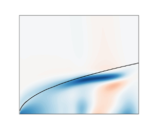
Workflow for sensitivity computation. Application to the second Mack mode in the  $M=4.5$ boundary layer. Mach number contours for base flow
 $\boldsymbol {\bar {q}}$. Real part of the streamwise momentum forcing for the optimal forcing
 $\boldsymbol {\check {f}}$. Real part of the pressure disturbances for the optimal response
 $\boldsymbol {\check {q}}$. Sensitivity of the optimal gain to streamwise momentum base-flow modifications contours for the sensitivity to base flow
 $\boldsymbol {\nabla }_{\boldsymbol {\bar {q}}} \mu ^2$.

2. Methods
After presenting the governing equations (§ 2.1), we recall briefly the definitions of a base flow and resolvent modes/optimal gains (§ 2.2). Then, we show the sensitivity of the optimal gains (§ 2.3) while the numerical details are given in § 2.5.
2.1. Governing equations
We consider the compressible Navier–Stokes equations written in conservative form
 \begin{equation} \frac{\partial \boldsymbol{q}}{\partial t} + \boldsymbol{\nabla}\boldsymbol{\cdot}\boldsymbol{F}(\boldsymbol{q}) = 0, \end{equation}
with  $\boldsymbol {q} = (\rho, \rho \boldsymbol {v}, \rho E)$ denoting, respectively, the density, momentum and total energy of the fluid and
 $\boldsymbol {F}(\boldsymbol {q})$ the associated fluxes. In expanded form, the Navier–Stokes equations read
 $$\begin{gather} \frac{\partial \rho}{\partial t} + \boldsymbol{\nabla} \boldsymbol{\cdot} ( \rho \boldsymbol{v} ) = 0, \end{gather}$$
 $$\begin{gather}\frac{\partial (\rho \boldsymbol{v})}{\partial t} + \boldsymbol{\nabla}\boldsymbol{\cdot} ( \rho \boldsymbol{v} \boldsymbol{v} + p \boldsymbol{I} - \boldsymbol{\tau} ) = 0, \end{gather}$$
 $$\begin{gather}\frac{\partial (\rho E)}{\partial t} + \boldsymbol{\nabla}\boldsymbol{\cdot} ( (\rho E +p) \boldsymbol{v} - \boldsymbol{\tau} \boldsymbol{\cdot} \boldsymbol{v} - \lambda \boldsymbol{\nabla} T ) = 0, \end{gather}$$
with  $E = p / (\rho (\gamma -1)) + \frac {1}{2}\boldsymbol {v} \boldsymbol {\cdot } \boldsymbol {v}$,
 $\boldsymbol {\tau } = \eta ( \boldsymbol {\nabla } \boldsymbol {v} + (\boldsymbol {\nabla } \boldsymbol {v})^{\rm T}) - \frac {2}{3} \eta (\boldsymbol {\nabla }\boldsymbol {\cdot } \boldsymbol {v}) \boldsymbol {I}$,
 $\boldsymbol {I}$ the identity tensor,
 $p$ the pressure,
 $\eta$ the dynamic viscosity,
 $\boldsymbol{v}$ the velocity, T the temperature,
 $\lambda = \eta c_p / Pr$,
 $c_p$ the isobaric heat capacity and
 $P_r$ the Prandtl number (
 $P_r = 0.72$). To close the system, two more equations are required. First, one assumes a homogeneous, thermally and calorically perfect gas. The perfect gas law is
 \begin{equation} p = \rho r T, \end{equation}
with  $r = 287.1\ \textrm {J}\ \textrm {kg}^{-1}\ \textrm {K}^{-1}$ the specific gas constant. Then, Sutherland's law is selected to link the viscosity
 $\eta$ to the temperature (Sutherland Reference Sutherland1893)
 \begin{equation} \eta (T) = \eta_{ref} \left( \frac{T}{T_{ref}} \right)^{3/2} \frac{T_{ref} + S}{T + S}, \end{equation}
with  $S = 110.4$ K the Sutherland temperature,
 $\eta _{ref} = 1.716 \times 10^{-5}\ \textrm {kg}\ \textrm {m}^{-1}\ \textrm {s}^{-1}$ and
 $T_{ref} = 273.15$ K.
After spatial discretisation (see § 2.5), the discrete residual is noted  $\boldsymbol {R}(\boldsymbol {q}) = - \boldsymbol {\nabla }\boldsymbol {\cdot }\boldsymbol {F}(\boldsymbol {q})$.
2.2. Base flow, resolvent modes and optimal gains
The boundary layer base flow  $\boldsymbol {\bar {q}}$ is a steady solution of the governing equations
 \begin{equation} \boldsymbol{R}(\boldsymbol{\bar{q}}) = 0. \end{equation}
It is an amplifier flow (Huerre & Monkewitz Reference Huerre and Monkewitz1990), for which all small-amplitude perturbations are exponentially stable in time (globally stable but convectively unstable). In such flows, it is more relevant to perform a resolvent analysis to study the linear dynamics of the flow and identify the pseudo-resonances of the flow. For this, we transform to frequency space and consider a small-amplitude forcing field  $\boldsymbol {f}'(t)={\rm e}^{{\rm i}\omega t} \boldsymbol {\check {f}}$ that is applied to the right-hand side of (2.1) and which may be restricted, through a prolongation matrix
 $\boldsymbol {P}$, to specific regions of the flow or specific components of the state. Here,
 $\boldsymbol {P}$ is a rectangular matrix, containing only zeros and ones, and of size equal to the dimension of the state
 $\boldsymbol {q}$ times the dimension of the forcing
 $\boldsymbol {f}$. The linear response of the flow
 $\boldsymbol {q}'(t)={\rm e}^{{\rm i}\omega t} \boldsymbol {\check {q}}$ is then governed by
 $\boldsymbol {\check {q}} = \boldsymbol {\mathcal {R} P \check {f}}$, with
 $\boldsymbol {\mathcal {R}} = ( {\rm i}\omega \boldsymbol {I} - \boldsymbol {A} )^{-1}$ denoting the resolvent operator,
 $\boldsymbol {A} = \partial \boldsymbol {R}/\partial \boldsymbol {q}$ the Jacobian and
 $\boldsymbol {I}$ the identity tensor. The resolvent operator corresponds to a transfer function between the input (forcing) and the response (perturbations). The optimal forcings/responses are then computed by optimising the input–output gain
 $\mu ^2$ between the energy of the response and the energy of the forcing
 \begin{equation} \mu^2 = \sup_{\boldsymbol{\check{f}}} \frac{\| \boldsymbol{\check{q}} \|^2_q}{\| \,\boldsymbol{\check{f}} \|^2_f}, \end{equation}
with  $\|{\cdot }\|_q$ and
 $\|{\cdot }\|_f$ the user-selected norms to evaluate the amplitude of the fluctuations and the forcing. These measures are defined with their associated discrete positive Hermitian matrices
 $\boldsymbol {Q}_q$ and
 $\boldsymbol {Q}_f$
 \begin{equation} \| \boldsymbol{\check{q}} \|^2_q = \boldsymbol{\check{q}}^* \boldsymbol{Q}_q \boldsymbol{\check{q}} , \quad \| \,\boldsymbol{\check{f}} \|^2_f = \boldsymbol{\check{f}}^* \boldsymbol{Q}_f \boldsymbol{\check{f}}, \end{equation}
where only  $\boldsymbol {Q}_f$ is required to be definite. For compressible flows, a common choice for
 $\boldsymbol {Q}_q$ and
 $\boldsymbol {Q}_f$ consists of Chu's energy (Chu Reference Chu1965) in order to take into account the pressure (
 $\check {p}$) and entropy (
 $\check {s}$) disturbances, which writes for dimensionless fluctuations
 \begin{equation} E_{Chu} = \boldsymbol{\check{q}}^* \boldsymbol{Q}_{Chu} \boldsymbol{\check{q}} = \frac{1}{2} \int_\varOmega \left( \bar{\rho}\|\boldsymbol{\check{v}}\|^2 + \frac{1}{\gamma}\frac{\check{p}^2}{ \bar{p}} + \gamma (\gamma -1) M^4\, \bar{p}\, \check{s}^2 \right) {\rm d}\varOmega. \end{equation}
Chu's energy is the sum of the kinetic energy of the perturbation and a thermodynamic component (potential energy from compression and from heat exchange) with appropriate coefficients to exclude the conservative compression work (Hanifi, Schmid & Henningson Reference Hanifi, Schmid and Henningson1996) in order to obtain a norm which does not increase in time in the absence of sources of energy (George & Sujith Reference George and Sujith2011). Matrix  $\boldsymbol {Q}_q = \boldsymbol {Q}_f = \boldsymbol {Q}_{Chu}$ for Chu's energy norm is block diagonal and may be written with conservative variables, as detailed in Appendix A.
Solving for  $\mu _i^2$ over a range of frequencies
 $\omega$ provides the most receptive frequency (where
 $\mu _i(\omega )^2$ is the largest) and the associated optimal forcing mode
 $\boldsymbol {\check {f}}_i$.
From an algorithmic point of view, we solve for the optimal gain in (2.8) by rewriting
 \begin{equation} \mu^2 = \sup_{ \boldsymbol{\check{f}}} \frac{\boldsymbol{\check{q}}^* {\boldsymbol{Q}_q} \boldsymbol{\check{q}} }{\boldsymbol{\check{f}}^* \boldsymbol{Q}_f \boldsymbol{\check{f}}} = \sup_{ \boldsymbol{\check{f}}} \frac{(\boldsymbol{\mathcal{R}P \check{f}})^* {\boldsymbol{Q}_q} (\boldsymbol{\mathcal{R}P \check{f}})}{(\boldsymbol{P \check{f}})^* \boldsymbol{Q}_f (\boldsymbol{P \check{f}})} = \sup_{ \boldsymbol{\check{f}}} \frac{ \boldsymbol{\check{f}}^* \boldsymbol{P}^* \boldsymbol{\mathcal{R}}^* {\boldsymbol{Q}_q} \boldsymbol{\mathcal{R}P \check{f}}}{ \boldsymbol{\check{f}}^* {\boldsymbol{Q}_f} \boldsymbol{\check{f}}}. \end{equation}
The optimisation problem defined by (2.11) is the Rayleigh quotient. It is equivalent to the generalised Hermitian eigenvalue problem
 \begin{equation} \boldsymbol{P}^* \boldsymbol{\mathcal{R}}^* {\boldsymbol{Q}_q} \boldsymbol{\mathcal{R}P \check{f}}_i = \mu_i^2 {\boldsymbol{Q}_f} \boldsymbol{\check{f}}_i. \end{equation}
Its eigenvalues are ranked such that  $\mu _i^2 \geq \mu _{i+1}^2$ and the associated eigenvectors are
 $\boldsymbol {\check {f}}_i$, which we normalise to
 $\boldsymbol {\check {f}}_i^* \boldsymbol {Q}_f \boldsymbol {\check {f}}_i=1$. The normalised responses (
 $\boldsymbol {\check {q}}_i^* \boldsymbol {Q}_q \boldsymbol {\check {q}}_i=1$) are then obtained through
 \begin{equation} \boldsymbol{\check{q}}_i = \mu_i^{-1}\boldsymbol{\mathcal{R} P \check{f}}_i. \end{equation}
The bases  $\boldsymbol {\check {f}}_i$ and
 $\boldsymbol {\check {q}}_i$ are orthonormal bases of the input and output spaces.
2.3. Sensitivity of optimal gains to base-flow variations, steady forcing and parameter variations
Linear sensitivity of eigenvalues to a general flow parameter has been addressed by Martínez-Cava (Reference Martínez-Cava2019). Here, we focus on optimal gains, as in Brandt et al. (Reference Brandt, Sipp, Pralits and Marquet2011). Following the discrete framework introduced in Mettot, Renac & Sipp (Reference Mettot, Renac and Sipp2014) for eigenvalues, we extend the work of Martínez-Cava (Reference Martínez-Cava2019) to optimal gains and emphasise the link with the concepts of linear sensitivity of the optimal gain to base-flow modifications  $\delta \boldsymbol {\bar {q}}$ and steady forcing
 $\delta \boldsymbol {\bar {f}}$, that were initially described in detail in Marquet, Sipp & Jacquin (Reference Marquet, Sipp and Jacquin2008). We consider the general case of the sensitivity of the optimal gain
 $\mu _i^2$ to any flow parameter written
 $\boldsymbol {p}$, such that
 \begin{equation} \delta\mu_i^2=(\boldsymbol{\nabla}_{\!\boldsymbol{p}} \mu_i^2)^*\boldsymbol{Q}_p\delta \boldsymbol{p}, \end{equation}
where  $\boldsymbol {Q}_p$ is a given scalar product. The parameter
 $\boldsymbol {p}$ can be either a scalar number as Reynolds number,
 $M$,
 $T_\infty,\ldots$ or a large-dimensional vector such as the prescribed inlet profile or control vectors (wall-normal velocity or wall-temperature profiles). The latter will be considered for application in the next section. The only restriction in the following is that the control parameter
 $\boldsymbol {p}$ has to be invariant in time and in the
 $z$-direction, as the base flow is assumed to remain steady and two-dimensional when varying the control parameter. We consider that the residual depends on the parameter
 ${p}$ i.e.
 $\boldsymbol {R}(\boldsymbol {q})=\boldsymbol {R}(\boldsymbol {q},\boldsymbol {p})$ and consequently also the Jacobian
 $\boldsymbol {A}(\boldsymbol {q},\boldsymbol {p}) = \partial \boldsymbol {R}(\boldsymbol {q},\boldsymbol {p}) / \partial \boldsymbol {q}$.
The objective of the optimisation is maximising the optimal gain  $\mu _i^2$ under the constraint given by the eigenvalue problem written in (2.12) and that the base flow is a solution of
 $\boldsymbol {R}(\boldsymbol {\bar {q}},\boldsymbol {p}) = 0$. Because of the space or component restriction (
 $\boldsymbol {P}$ may be degenerate), it is necessary to split the generalised eigenvalue problem (2.12) into three equations in order to handle only matrices without inverses
 \begin{equation} \boldsymbol{P\check{f}}_i = \mu_i ({\rm i}\omega\boldsymbol{I}-\boldsymbol{A})\boldsymbol{\check{q}}_i, \quad \mu_i \boldsymbol{Q}_q \boldsymbol{\check{q}}_i = (-{\rm i}\omega\boldsymbol{I}-\boldsymbol{A}^*) \boldsymbol{\check{a}}, \quad \boldsymbol{P}^*\boldsymbol{\check{a}} = \mu_i^2 \boldsymbol{Q}_f\boldsymbol{\check{f}}_i. \end{equation}
This system involves an additional component  $\boldsymbol {\check {a}}$ within the eigenproblem. We therefore define the Lagrangian function
 $\mathcal {L}$ as a function of the state (the optimal gain
 $\mu _i^2$, the optimal forcing
 $\boldsymbol {\check {f}}_i$ and response
 $\boldsymbol {\check {q}}_i$, the additional variable
 $\boldsymbol {\check {a}}$, the base flow
 $\boldsymbol {\bar {q}}$), the four Lagrangian multipliers
 $\boldsymbol {\lambda }_1$,
 $\boldsymbol {\lambda }_2$,
 $\boldsymbol {\lambda }_3$ and
 $\boldsymbol {\lambda }_4$ and the control vector
 $\boldsymbol {p}$
 \begin{align} \mathcal{L}([\mu_i^2,\boldsymbol{\check{f}}_i,\boldsymbol{\check{q}}_i,\boldsymbol{\check{a}},\boldsymbol{\bar{q}}],\boldsymbol{\lambda}_{1\cdots4},\boldsymbol{p}) &= \mu_i^2 + \langle \boldsymbol{\lambda}_1, \boldsymbol{P\check{f}}_i- \mu_i ({\rm i}\omega\boldsymbol{I}-\boldsymbol{A}(\boldsymbol{\bar{q}},\boldsymbol{p}))\boldsymbol{\check{q}}_i \rangle \nonumber\\ &\quad + \langle \boldsymbol{\lambda}_2 , \mu_i\boldsymbol{Q}_q(\boldsymbol{\bar{q}}) \boldsymbol{\check{q}}_i + ({\rm i}\omega\boldsymbol{I}+\boldsymbol{A}(\boldsymbol{\bar{q}},\boldsymbol{p})^*) \boldsymbol{\check{a}} \rangle \nonumber\\ &\quad + \langle \boldsymbol{\lambda}_3 , \boldsymbol{P}^*\boldsymbol{\check{a}} - \mu_i^2 \boldsymbol{Q}_f(\boldsymbol{\bar{q}})\boldsymbol{\check{f}}_i \rangle + \langle \boldsymbol{\lambda}_4, \boldsymbol{R}(\boldsymbol{\bar{q}},\boldsymbol{p}) \rangle. \end{align}
Here,  $\langle \boldsymbol {a},\boldsymbol {b} \rangle = \boldsymbol {a}^*\boldsymbol {b}$ is the Hermitian scalar product. By zeroing the variation of
 $\mathcal {L}$ with the state, taking into account that
 $\langle \,\boldsymbol {\check {f}}_i, \boldsymbol {Q}_f \boldsymbol {\check {f}}_i \rangle =1$, we obtain that
 \begin{equation} \boldsymbol{\lambda}_1= \boldsymbol{\check{a}}, \quad \boldsymbol{\lambda}_2 =\mu_i \boldsymbol{\check{q}}_i, \quad \boldsymbol{\lambda}_3 = \boldsymbol{\check{f}}_i, \quad \boldsymbol{\lambda}_4 = \boldsymbol{Q}_f\boldsymbol{\nabla}_{\boldsymbol{\bar{f}}} \mu_i^2, \end{equation}
where
 $$\begin{gather} \frac{\boldsymbol{\nabla}_{\boldsymbol{\bar{f}}} \mu_i^2}{\mu_i^2}=- \boldsymbol{Q}_f^{-1}\boldsymbol{A}^{-1*}\boldsymbol{Q}_q \frac{\boldsymbol{\nabla}_{\boldsymbol{\bar{q}}} \mu_i^2}{\mu_i^2}, \end{gather}$$
 $$\begin{gather}\frac{\boldsymbol{\nabla}_{\boldsymbol{\bar{q}}} \mu_i ^2}{\mu_i^2} = \boldsymbol{Q}_q^{-1} \left[2\,{\rm Re}\left( \boldsymbol{H}'^* \boldsymbol{\mathcal{R}}^{*}\boldsymbol{Q}_q \boldsymbol{\check{q}}_i \right) + \left( \frac{\partial (\boldsymbol{Q}_q \boldsymbol{\check{q}}_i)}{\partial \boldsymbol{q}} \right)^* \boldsymbol{\check{q}}_i - \left( \frac{\partial (\boldsymbol{Q}_f \boldsymbol{\check{f}}_i)}{\partial \boldsymbol{q}} \right)^* \boldsymbol{\check{f}}_i\right], \end{gather}$$
are two vectors called sensitivity to steady volume forcing and sensitivity to base-flow variations (Marquet et al. Reference Marquet, Sipp and Jacquin2008; Brandt et al. Reference Brandt, Sipp, Pralits and Marquet2011; Mettot et al. Reference Mettot, Renac and Sipp2014) that satisfy
 \begin{equation} \delta \mu_i^2 = (\boldsymbol{\nabla}_{\boldsymbol{\bar{f}}} \mu_i^2)^* \boldsymbol{Q}_f \delta\boldsymbol{\bar{f}} = (\boldsymbol{\nabla}_{\boldsymbol{\bar{q}}} \mu_i^{2})^* \boldsymbol{Q}_q \delta \boldsymbol{\bar{q}}. \end{equation}
Matrix  $\boldsymbol {H}'$ is defined as
 $\boldsymbol {H}' \delta \boldsymbol {\bar {q}}= \boldsymbol {H}(\boldsymbol {\check {q}}_i, \delta \boldsymbol {\bar {q}})$ for all
 $\delta \boldsymbol {\bar {q}}$, where
 $\boldsymbol {H}={\partial \boldsymbol {A}}/{\partial \boldsymbol {q}}={\partial ^2 \boldsymbol {R}}/{\partial \boldsymbol {q}^2}$ is the Hessian rank-3 tensor. Details of the computation of the sensitivity to base-flow modifications is given in Appendix B.
In expression (2.19), the components  ${\partial \boldsymbol {Q}_{q,f}}/{\partial \boldsymbol {q}}$ are non-zero in the case of Chu's energy norm. As an aside, Brandt et al. (Reference Brandt, Sipp, Pralits and Marquet2011) has introduced an additional physical constraint (the time-invariant continuity equation (2.2)) to study the sensitivity to physically relevant base-flow modifications. Details of the computation of the sensitivity to momentum-divergence-free base-flow modifications is given in Appendix C.
Finally, the variation of  $\mathcal {L}$ with the control vector
 $\boldsymbol {p}$ provides the gradient of interest
 \begin{equation} \frac{\boldsymbol{\nabla}_{\!\boldsymbol{p}} \mu_i^2}{\mu_i^2} = \boldsymbol{Q}_p^{-1} \left[ \left(\frac{\partial \boldsymbol{R}}{\partial \boldsymbol{p}}\right)^* \boldsymbol{Q}_f \frac{\boldsymbol{\nabla}_{\boldsymbol{\bar{f}}} \mu_i^2}{\mu_i^2} + 2 \,{\rm{Re}}\left( \boldsymbol{\tilde{H}}'^* \boldsymbol{\mathcal{R}}^{*}\boldsymbol{Q}_q \boldsymbol{\check{q}} \right) \right], \end{equation}
with  $\boldsymbol {\tilde {H}}'$ defined as
 $\boldsymbol {\tilde {H}}' \delta \boldsymbol {p} = \boldsymbol {\tilde {H}} (\boldsymbol {\check {q}}_i, \delta \boldsymbol {p})$ for all
 $\delta \boldsymbol {p}$,
 $\boldsymbol {\tilde {H}}={\partial \boldsymbol {A}}/{\partial \boldsymbol {p}}={\partial ^2 \boldsymbol {R}}/{\partial \boldsymbol {q}\partial \boldsymbol {p}}$ being a rank-3 tensor.
In expression (2.21), the first term is interpreted as the variation of the optimal gain induced by the modification of the Jacobian due to the change of the base flow  $\boldsymbol {A}(\boldsymbol {q})$ while the second term is the variation of the Jacobian due to the variation of the control parameter
 $\boldsymbol {A}(\boldsymbol {p})$, keeping the base flow constant. It has been described in a similar context in Guo et al. (Reference Guo, Gao, Jiang and Lee2021) for eigenvalue sensitivity: route I is the distortion of the base flow which induces a modification of the eigenvalue problem, route II is the direct distortion of the linear operator. Depending on the parameter
 $\boldsymbol {p}$ chosen to compute the sensitivity, one route or another is favoured.
2.4. Interpretation of  $\boldsymbol {\nabla }_{\boldsymbol {p}}\mu _i^2$ and $\boldsymbol {\nabla }_{\bar {\boldsymbol {q}}} \mu _i^2$


We consider the following optimisation problem:
 \begin{equation} \delta\boldsymbol{p}^{m}=\operatorname{argmax}_{\| \delta\boldsymbol{p} \|_{p} =1} \delta \mu_i^2(\delta\boldsymbol{p}), \end{equation}
where  $\delta \mu _i^2$ and
 $\delta {\boldsymbol {p}}$ are related through (2.14) and
 $^m$ indicates the optimal (maximal) parietal vector. It is straightforward to show that
 \begin{equation} \delta\boldsymbol{p}^{m}=\frac{\boldsymbol{\nabla}_{\!\boldsymbol{p}}\mu_i^2}{\| \boldsymbol{\nabla}_{\!\boldsymbol{p}}\mu_i^2\|_p}. \end{equation}
The gradient is therefore the best profile (of given small amplitude measured with  $\| {\cdot } \|_p$) that optimally increases the gain and therefore optimally strengthens the instability. Conversely, because of linearity,
 $-\delta \boldsymbol {p}^{m}$ is the optimal open-loop control to damp the optimal gain.
For interpretation,  $\delta \mu _i^2|^{m}:=\delta \mu _i^2 ( \delta \boldsymbol {p}^{m})$ may be rewritten as
 \begin{equation} \frac{\delta \mu_i^2|^{m}}{\mu_i^2} =\underbrace{\left[2 \boldsymbol{Q}_p^{-1}\,{\rm Re}\left( \boldsymbol{\tilde{H}}'^* \boldsymbol{\mathcal{R}}^{*}\boldsymbol{Q}_q \boldsymbol{\check{q}} \right)\right]^* \boldsymbol{Q}_p \delta \boldsymbol{p}^{m}}_{\delta E^{m}_{\boldsymbol{A}}} +\underbrace{\left(\frac{\boldsymbol{\nabla}_{\boldsymbol{\bar{q}}} \mu_i^{2}}{\mu_i^2}\right)^* \boldsymbol{Q}_q \delta \boldsymbol{\bar{q}}^{m}}_{\delta E^{m}_{\boldsymbol{\bar{q}}}}, \end{equation}
where the first term on the right-hand side,  $\delta E^{m}_{\boldsymbol {A}}$, is the variation of the gain due to the induced modification of the Jacobian, and the second part,
 $\delta E^{m}_{\boldsymbol {q}}$, is the variation due to the induced change in base flow
 \begin{equation} \delta\bar{\boldsymbol{q}}^{m}=-\boldsymbol{A}^{-1}\left(\frac{\partial \boldsymbol{R}}{\partial \boldsymbol{p}}\right)\delta\boldsymbol{p}^{m}. \end{equation}
Finally, the optimal gain variation due to the induced base-flow modification may be broken down into three pieces
 \begin{equation} \delta E^{m}_{\boldsymbol{\bar{q}}}=\delta E^{m}_k+\delta E^{m}_p+\delta E^{m}_s, \end{equation}
where
 \begin{equation} \left.\begin{gathered} \delta E^{m}_k=\int_\varOmega \frac{\bar{\rho}\delta{\boldsymbol{\bar{v}}}^{b} \boldsymbol{\cdot}\delta{\boldsymbol{\bar{v}}}^{m}}{2} {\rm d}\varOmega, \quad \delta E^{m}_p=\int_\varOmega \frac{\delta\bar{p}^{b}\delta\bar{p}^{m}}{2\gamma\bar{p}} {\rm d}\varOmega, \\ \delta E^{m}_s=\frac{\gamma(\gamma-1)M^4}{2}\int_\varOmega \bar{p}\delta{{\bar{s}}}^{b}\delta{{\bar{s}}}^{m} \,{\rm d}\varOmega. \end{gathered}\right\} \end{equation}
Here, the notation  $(\delta {\boldsymbol {\bar {v}}}^{b},\delta {\bar {p}^{b}},\delta {{\bar {s}}^{b}})$ corresponds to the velocity–pressure–entropy variations associated with
 $\delta {\boldsymbol {\bar {q}}}^{b}:={\boldsymbol {\nabla }_{\boldsymbol {\bar {q}}} \mu _i^{2}}/{\mu _i^2}$, with
 $^b$ denoting the optimal base-flow modification vector, and
 $(\delta {\boldsymbol {\bar {v}}}^{m},\delta {{\bar {p}}}^{m},\delta {{\bar {s}}}^{m})$ to
 $\delta \bar {\boldsymbol {q}}^{m}$. In the following, we will represent the contributions
 $\delta E^{m}_{\boldsymbol {A}}$,
 $\delta E^{m}_k$,
 $\delta E^{m}_p$ and
 $\delta E^{m}_s$ to assess the importance of Jacobian, base-flow kinetic energy, pressure and entropy modifications in the gain variation associated with the optimal control
 $\delta \boldsymbol {p}^{m}$.
Finally, it is also straightforward to show that the above  $\delta \boldsymbol {\bar {q}}^{b}$ is also the solution to the following optimisation problem:
 \begin{equation} \delta\boldsymbol{\bar{q}}^{b}=\operatorname{argmax}_{\| \delta\boldsymbol{\bar{q}} \|_{q} =\| \mu_i^{-2}\boldsymbol{\nabla}_{\bar{q}}\mu_i^2\|_q} \delta \mu_i^2(\delta\boldsymbol{\bar{q}}), \end{equation}
where  $\delta \mu _i^2$ and
 $\delta \boldsymbol {\bar {q}}$ are related through (2.20). Hence, the maximum
 $\delta \mu _i^2|^{b}:=\delta \mu _i^2 ( \delta \boldsymbol {\bar {q}}^{b})$, can be rewritten and decomposed as
 \begin{equation} \frac{\delta \mu_i^2|^{b}}{\mu_i^2}=\left\| \frac{\boldsymbol{\nabla}_{\bar{q}}\mu_i^2}{\mu_i^{2}}\right\|_q^2={ \delta E^{b}_k + \delta E^{b}_p + \delta E^{b}_s } ,\end{equation}
where
 \begin{equation} \delta E^{b}_k=\int_\varOmega \frac{\bar{\rho}\|\delta{\boldsymbol{\bar{v}}}^{b}\|^2}{2} {\rm d}\varOmega, \quad \delta E^{b}_p=\int_\varOmega \frac{\left(\delta\bar{p}^{b}\right)^2}{2\gamma\bar{p}} {\rm d}\varOmega, \quad \delta E^{b}_s=\frac{\gamma(\gamma-1)M^4}{2}\int_\varOmega \bar{p}\left(\delta{{\bar{s}}}^{b}\right)^2 \,{\rm d}\varOmega. \end{equation}
In the following, we will represent the contributions  $\delta E^{b}_k$,
 $\delta E^{b}_p$ and
 $\delta E^{b}_s$ to assess the importance of base-flow kinetic energy, pressure and entropy modifications in the gain variation associated with the base-flow modification
 $\delta {\bar {\boldsymbol {q}}}^{b}$.
2.5. Numerical methods
2.5.1. Numerical discretisation and algorithms
The BROADCAST code includes all the tools required to compute the base flow, the global stability analysis and the linear sensitivity analysis. A detailed description of the various numerical methods and their validation for stability and sensitivity in BROADCAST can be found in Poulain et al. (Reference Poulain, Content, Sipp, Rigas and Garnier2023).
The two-dimensional space discretisation for the inviscid flux follows the seventh-order FE-MUSCL (flux-extrapolated monotonic upstream-centred scheme for conservation laws) scheme (Cinnella & Content Reference Cinnella and Content2016) which had been assessed in hypersonic flow simulations by Sciacovelli et al. (Reference Sciacovelli, Passiatore, Cinnella and Pascazio2021), showing excellent results in accuracy and shock capturing features. The viscous fluxes are computed on a five-point compact stencil which is fourth-order accurate (Shen, Zha & Chen Reference Shen, Zha and Chen2009).
The Jacobian as well as all the other operators derived to compute the gradients are constructed by algorithmic differentiation (AD) through the software TAPENADE (Hascoet & Pascual Reference Hascoet and Pascual2013). The matrix operators are explicitly built by matrix-vector products (Mettot Reference Mettot2013). They correspond to linearised discrete residuals given by AD and are stored in a sparse format. For sensitivity computation, for instance in the case of the wall velocity ( $\boldsymbol {p}=\boldsymbol {v}_w$), the numerical method to compute the sparse residual and Jacobian operators
 $\partial \boldsymbol {R} / \partial \boldsymbol {v}_w$ and
 $\partial \boldsymbol {A} / \partial \boldsymbol {v}_w$ which appear in
 $\boldsymbol {\nabla }_{\boldsymbol {v}_w} \mu ^2$ consists of writing the wall-boundary condition which appears inside the residual
 $\boldsymbol {R}$ as a function of the input
 $\boldsymbol {v}_w$ (taken equal to
 $0$ for base flow) and linearising through AD. A description of the implementation of the wall-boundary condition is given in Appendix D.
All linear systems involving sparse matrices are then solved using the PETSC software interface (Balay et al. Reference Balay2019) which includes the direct sparse lower-upper decomposition (LU) solver from MUMPS (Amestoy et al. Reference Amestoy, Duff, L'Excellent and Koster2001). With the BROADCAST code being written in the Python language, the petsc4py version is used (Dalcin et al. Reference Dalcin, Paz, Kler and Cosimo2011). The base-flow solution is solved with a Newton method which consists of an iterative method, where from a state  $\boldsymbol {q}^n$, we build
 $\boldsymbol {q}^{n+1} = \boldsymbol {q}^n + \delta \boldsymbol {q}^n$, with
 $\boldsymbol {A}(\boldsymbol {q}^n)\, \delta \boldsymbol {q}^n = - \boldsymbol {R}(\boldsymbol {q}^n)$ and
 $\boldsymbol {A}(\boldsymbol {q}^n) ={\partial \boldsymbol {R}}/{\partial \boldsymbol {q}} |_{\boldsymbol {q}^n}$ is the Jacobian operator evaluated at
 $\boldsymbol {q}=\boldsymbol {q}^n$. To ease convergence, a pseudo-transient continuation method (or relaxation method) is used following Crivellini & Bassi (Reference Crivellini and Bassi2011). To solve the generalised eigenvalue problem from resolvent analysis, we use the SLEPc library (Roman et al. Reference Roman, Campos, Romero and Tomás2015), which implements various Krylov–Schur methods (Hernández et al. Reference Hernández, Román, Tomás and Vidal2007).
The gradients do not depend on the domain height, given that the full forcing/response support is included in the domain, and have been validated by comparing the results with a finite difference method
 \begin{equation} \lim_{\epsilon \rightarrow 0}\frac{\mu_i^2(\boldsymbol{p} + \epsilon \boldsymbol{\nabla}_{\!\boldsymbol{p}} \mu_i^2) - \mu_i^2(\boldsymbol{p})}{\epsilon} \rightarrow \| \boldsymbol{\nabla}_{\!\boldsymbol{p}} \mu_i^2\|^2. \end{equation}
Furthermore, a comparison of the gradient of the optimal gain with wall blowing between the discrete and continuous frameworks is performed on a low Mach boundary layer in Appendix E.
2.5.2. Building the Jacobian and Hessian for three-dimensional perturbations
The extension of global stability analysis to linear three-dimensional (3-D) perturbations follows Bugeat et al. (Reference Bugeat, Chassaing, Robinet and Sagaut2019) and has been adapted to BROADCAST in Poulain et al. (Reference Poulain, Content, Sipp, Rigas and Garnier2023). The base flow being homogeneous in the  $z$-direction, the perturbation field can be searched under the form
 \begin{equation} \boldsymbol{q}'(x,y,z,t) = \boldsymbol{\check{q}}(x,y) \exp({{\rm i}(\omega t + \beta z)}), \end{equation}
where  $\beta$ is the real wavenumber in the
 $z$-direction. A similar form is assumed for the optimal forcing. These perturbations can therefore be studied on the same 2-D mesh without discretisation of the
 $z$-direction. The
 $z$-dependency of the forcing and response are taken into account analytically. One can split the 3-D residual
 $\boldsymbol {R}_\textrm {3D}$ as the sum of the 2-D discretised residual
 $\boldsymbol {R}$ and its
 $z$-derivative components
 $\boldsymbol {R}_z$
 \begin{equation} \boldsymbol{R}_\text{3D} (\boldsymbol{q}) = \boldsymbol{R} (\boldsymbol{q}) + \boldsymbol{R}_z(\boldsymbol{q}). \end{equation}
For the compressible Navier–Stokes equations, the  $\boldsymbol {R}_z$ residual in conservative form can be written as the sum of four functions whose expressions can be found in Poulain et al. (Reference Poulain, Content, Sipp, Rigas and Garnier2023)
 \begin{equation} \boldsymbol{R}_z (\boldsymbol{q}) = \boldsymbol{B}(\boldsymbol{q}) \frac{\partial \boldsymbol{q}}{\partial z} + \boldsymbol{C}_1(\boldsymbol{q}) \frac{\partial^2 \boldsymbol{q}}{\partial z^2} + \frac{\partial \boldsymbol{C}_2}{\partial \boldsymbol{q}} \frac{\partial \boldsymbol{q}}{\partial z} \frac{\partial \boldsymbol{q}}{\partial z} + \boldsymbol{D}_1(\boldsymbol{q}) \frac{\partial \boldsymbol{q}}{\partial z} \odot \boldsymbol{D}_2(\boldsymbol{q}) \frac{\partial \boldsymbol{q}}{\partial z}. \end{equation}
Notation  $\odot$ refers to the element-wise product of two matrices or vectors (Hadamard product). Given that the base flow is homogeneous in the
 $z$-direction and keeping only the first-order terms for small fluctuations
 $\boldsymbol {q}'$, the linearisation of (2.33) yields
 \begin{equation} \boldsymbol{A}_\text{3D}\, (\boldsymbol{\bar{q}}) \boldsymbol{q}' = (\boldsymbol{A}(\boldsymbol{\bar{q}}) + \boldsymbol{A}_z(\boldsymbol{\bar{q}}) )\, \boldsymbol{q}' = (\boldsymbol{A}(\boldsymbol{\bar{q}}) + {\rm i}\beta \boldsymbol{B}(\boldsymbol{\bar{q}}) - \beta^2 \boldsymbol{C}_1(\boldsymbol{\bar{q}}) )\boldsymbol{q}'. \end{equation}
Linear sensitivity described in § 2.3 may also be extended to 3-D perturbations. However, the following expansions are correct only for 2-D sensitivity (homogeneous gradient in the  $z$-direction) of the eigenvalue/optimal gain of 3-D modes. Similarly to the equation (2.35), the 3-D Hessian operator can be written as
 $\boldsymbol {H}_\textrm {3D}(\boldsymbol {\check {q}},\boldsymbol {\bar {q}}) = \boldsymbol {H}(\boldsymbol {\check {q}},\boldsymbol {\bar {q}}) + \boldsymbol {H}_z(\boldsymbol {\check {q}},\boldsymbol {\bar {q}})$. One should notice that the base flow
 $\boldsymbol {\bar {q}}$ remains two-dimensional and only the response
 $\boldsymbol {\check {q}}$ brings a new 3-D contribution. The 3-D Hessian is defined as
 \begin{equation} \boldsymbol{H}_\text{3D}(\boldsymbol{\check{q}},\boldsymbol{\bar{q}}) = \left.\frac{\partial \left( \boldsymbol{A}_\text{3D} \boldsymbol{\check{q}} \right)}{\partial \boldsymbol{q}}\right|_{\boldsymbol{\bar{q}}}. \end{equation}
From (2.35), the following expression may be derived:
 \begin{equation} \boldsymbol{H}_\text{3D}' = \boldsymbol{H}' + {\rm i}\beta \frac{\partial \boldsymbol{B}}{\partial \boldsymbol{q}} \boldsymbol{\check{q}} - \beta^2 \frac{\partial \boldsymbol{C}_1}{\partial \boldsymbol{q}} \boldsymbol{\check{q}}. \end{equation}
Therefore, the 2-D sensitivity of a 3-D mode is given by the same equations as the one of a 2-D mode but by replacing the 2-D Hessian by the 3-D Hessian written in (2.37).
3. Supersonic boundary layer
3.1. Configuration and base flow
We consider an adiabatic flat plate close to the configuration studied in Bugeat et al. (Reference Bugeat, Chassaing, Robinet and Sagaut2019). All quantities are made non-dimensional with the following density, velocity, length and temperature scales:  $\rho _\infty$,
 $U_\infty$,
 $\nu _\infty /U_\infty$,
 $T_\infty$. The free-stream Mach number and free-stream temperature are respectively
 $M=4.5$ and
 $T_\infty = 288$ K. The spatial coordinates
 $(x,y,z)$ then correspond to
 $(Re_x, Re_y, Re_z)$, where, for example,
 $Re_x=U_\infty x /\nu _\infty$.
The flat-plate geometry is studied in a rectangular computational domain. The domain starts with a thin boundary layer profile at  $Re_{x,{in}} = 8160$ and ends at
 $Re_{x,{out}} = 2 \times 10^6$. The height of the domain is high enough in order not to affect the development of the boundary layer or the stability analysis. In practice, the domain height is approximately
 $9\,\delta ^*_{out}$ with
 $\delta ^*_{out}$ the compressible displacement thickness at the outlet. This gives
 $Re_{y,{top}} = 119\,000$. The Cartesian mesh is equi-spaced in the
 $x$-direction and stretched in the wall-normal direction (
 $y$-direction). The stretching has the following properties: maximum
 $y^+ \leqslant 1$ at the wall, cell height geometric growth rate of
 $2\,\%$ from
 $y=0$ to
 $y=3\delta _{99}$ with
 $\delta _{99}$ the boundary layer thickness, where
 $\Delta y^+ \approx 10$ is reached and then a growth rate increase from
 $2\,\%$ to
 $10\,\%$ from
 $y=3\delta _{99}$ to
 $y=L_y$ where
 $\Delta y^+ \approx 130$. The mesh has the size
 $(N_x, N_y) = (1000, 150)$ which gives
 $N = 150\,000$ grid points.
Four different boundary conditions are applied around the rectangular domain. At the inlet, a Dirichlet boundary condition is applied. The imposed flow profile corresponds to a compressible self-similar solution for  $u$,
 $v$,
 $\rho$ and
 $T$. At the outlet, an extrapolation boundary condition is imposed (the flow is overall assumed supersonic). An adiabatic no-slip wall is prescribed at the bottom while a non-reflecting condition (Poinsot & Lele Reference Poinsot and Lele1992) is employed at the top boundary.
The two-dimensional steady base flow (figure 2) is computed by a pseudo-transient continuation method, the compressible self-similar solution being taken as initial state. The algorithm converges in 7 iterations (high initial CFL (Courant–Friedrichs–Lewy number) as the self-similar solution is close to the base-flow solution) and decreases the residual  $L^2$ norms by 12 orders of magnitude.
Mach number field of the base flow. Solid line indicates the boundary layer thickness  $\delta _{99}$. Dashed line indicates the displacement thickness
 $\delta ^*$.

3.2. Stability
The global stability (resolvent) analysis of the  $M=4.5$ boundary layer over an adiabatic flat plate has been thoroughly studied by Bugeat et al. (Reference Bugeat, Chassaing, Robinet and Sagaut2019) and validated with the present tools in Poulain et al. (Reference Poulain, Content, Sipp, Rigas and Garnier2023). Therefore, more details can be found in the first cited paper, and only the most important stability results are recalled here because they represent necessary steps to perform the sensitivity analysis.
We recall that the frequency is normalised as  $F = \omega \nu _\infty / U_\infty ^2$ and the spanwise wavenumber
 $\beta$ with the reference length
 $\nu _\infty /U_\infty$. The measures
 $\boldsymbol {Q}_q$ and
 $\boldsymbol {Q}_f$ correspond to Chu's energy, both being restricted through
 $\boldsymbol {P}$ to
 $Re_{x} \leqslant 1.75 \times 10^6$ and
 $Re_y \leqslant 59\,500$ to remove the top and outlet boundary conditions from the optimisation domain. The forcing
 $\check {\boldsymbol {f}}$ is therefore only defined in this region and is applied to all five equations. At
 $M=4.5$, the second Mack mode exhibits a large gain,
 $\mu _0 = 1.80 \times 10^{7}$, which is obtained for
 $\beta =0$ and
 $F=2.3 \times 10^{-4}$. The optimal gains are also computed with
 $\beta \neq 0$ (figure 3a). The 3-D gains highlight streaks (
 $\mu _0 = 4.66 \times 10^{7}$) around
 $\beta = 2 \times 10^{-4}$ at zero frequency and the first oblique Mack mode is the strongest instability (
 $\mu _0 = 1.16 \times 10^{8}$) for approximately
 $\beta = 1.2 \times 10^{-4}$ and
 $F=3 \times 10^{-5}$.
Resolvent analysis. (a) Optimal gain  $\mu _0$ with respect to the frequency
 $F$ and the spanwise wavenumber
 $\beta$. White circle denotes the first Mack mode, black triangle the streaks and black square the second Mack mode. (b) Energy density
 $d_{Chu}$ of the optimal forcing (dashed lines) and response (solid lines) of the streaks (blue), the first (red) and second (green) Mack modes. Black vertical lines indicate branch I of first Mack mode (dashed line), branch I of the mode
 $S$ linked to the second Mack mode (dotted line), branch II of the same mode
 $S$ (dashed-dotted line) and the end of the optimisation domain for resolvent analysis (solid line).

The streamwise evolution of the resolvent modes is illustrated through their streamwise energy growth. An energy density is defined as the integral of Chu's energy in the wall-normal direction. For example,  $d_{Chu} (x) = \int _0^{y_{max}} \check {\boldsymbol {q}}(x,y)^* \boldsymbol {Q}_{Chu}(x,y)\check {\boldsymbol {q}}(x,y)\,{\textrm {d}y}$ for the optimal response. Chu's energy densities of the forcing and response for the streaks, first and second Mack modes are plotted in figure 3(b). A spatial local stability analysis (description of the method in Appendix F) has been performed at the frequency (
 $\omega$) and wavenumber (
 $\beta$) of the first and second Mack modes (see symbols in figure 3a). The streamwise locations of branch I (respectively II) which is the beginning (respectively end) of the unstable region in the
 $x$-direction of the local modes are also plotted in figure 3(b). The maximal optimal forcing locations for the first and second Mack modes agree well with the branch I location of their respective local modes. Branch II of the first Mack mode is downstream of the domain end while branch II of the local mode
 $S$ (linked to the second Mack mode) is slightly upstream of the maximal optimal response location of the second Mack mode. As suggested by Sipp & Marquet (Reference Sipp and Marquet2013), the discrepancies between local branches and maxima of the resolvent analysis are explained both by non-parallel effects (Gaster Reference Gaster1974) and Orr mechanism, the non-modal non-parallel unstable region being therefore larger than the local modal one. Furthermore, in comparison with the first Mack mode, larger differences between local and resolvent analyses are noticed for the second (higher frequency) where the Orr mechanism is stronger (Sipp & Marquet Reference Sipp and Marquet2013).
3.3. Sensitivity to wall-boundary control
After the computation of the sensitivity to base-flow modifications and steady forcing in Appendix G, whose results in the global framework match those of the literature on LST (Park & Zaki Reference Park and Zaki2019; Guo et al. Reference Guo, Gao, Jiang and Lee2021), the sensitivity of the streaks, first and second Mack modes to two types of modifications of the wall-boundary condition are analysed:
(i) Small-amplitude wall-normal blowing/suction
$\delta v_w(x)$ at the surface of the flat plate (Appendix H).(ii) Small-amplitude heat flux
$\delta \phi _w(x)$ at the surface of the flat plate (§ 3.4).


In both cases, the identity  $\boldsymbol {Q}_p = \boldsymbol {I}$ is chosen for the norm associated with the parameter spaces
 $\boldsymbol {p}=v_w$ and
 $\boldsymbol {p}=\phi _w$ as the discretisation along the
 $x$-direction is uniform.
In the following, we discuss the opposite of the sensitivity  $-\delta \boldsymbol {p}^m$ (see (2.23)), which corresponds to the optimal wall profile to be prescribed at the surface in order to mitigate the instability. This profile is plotted for blowing/suction control in figure 4(a) and for heat-flux control in figure 4(b). In figure 4, the marker ‘max. Forc.’ refers to the maximal optimal forcing location of the first Mack mode, ‘branch I’ to the streamwise location of branch I of the local mode linked to the first Mack mode and ‘max. ampli.’ to the location of the maximal amplification rate (
 $\max (-\alpha _i)$) of the local mode.
Optimal wall-control profiles to damp the different instabilities i.e. opposite of the sensitivity of the optimal gain for each instability:  $-\delta \boldsymbol {p}^m$. (a) Optimal wall-velocity profile
 $-\delta \boldsymbol {v}_w$. (b) Optimal wall heat-flux profile
 $-\delta \boldsymbol {\phi }_w$.

Both wall velocity and heat-flux control gradients highlight that the streaks are not sensitive to boundary control in comparison with the Mack modes. Furthermore, the profile to damp the streaks has a similar behaviour for both types of wall control i.e. negative in the downstream part of the domain where the optimal response of the streaks lies. In figure 4(a), the second Mack mode is confirmed to be the most sensitive instability to wall-velocity control. Furthermore, it is the only instability among the three which is stabilised by steady wall blowing (downstream  $Re_x = 1.2 \times 10^6$). The gradient for the second Mack mode is studied in detail in Appendix H. Optimal suction actuator locations to stabilise each instability are different:
 $Re_x = 0.6 \times 10^6$ for the first Mack mode (close to the location of the maximal amplification rate of the local mode),
 $Re_x = 1 \times 10^6$ for the second Mack mode and
 $Re_x = 1.7 \times 10^6$ for the streaks. However, a suction actuator located anywhere upstream
 $Re_x = 1.2 \times 10^6$ would damp both Mack modes without affecting much the streaks. The effect of applying the second Mack mode gradient on the stability of the other instabilities is investigated in § 3.5, where the design of an optimal wall-control actuator is attempted.
In figure 4(b), it is seen that the first Mack mode is the most sensitive to wall heat flux control. The profile to damp the optimal gain of the first Mack mode has one heating zone upstream until  $Re_x = 0.21 \times 10^6$ (located slightly downstream of branch I) and one cooling region downstream with the largest sensitivity close to the location of the maximal amplification rate of the local mode. The variations of the optimal wall heat-flux profile to damp the second Mack mode are more complex and are studied in detail in § 3.4. By comparing both Mack modes’ wall heat-flux profiles, they overall display an opposite behaviour with respect to wall heat-flux changes (Mack Reference Mack1993), however, in some streamwise regions, they follow similar trends. First, at the leading edge, upstream
 $Re_x = 0.21 \times 10^6$, heating the wall would damp both Mack modes and secondly, downstream, between
 $Re_x = 1.045 \times 10^6$ and
 $Re_x = 1.33 \times 10^6$, cooling would produce the same effect. The effect of the application of the first Mack mode gradient on the stability of the other instabilities is investigated in § 3.5. Furthermore, based on the zones where the gradients’ sign matches between the first and second Mack modes, a control that damps both instabilities will also be discussed in this section.
One may remark that the optimal wall-control profiles given by figure 4 may have been partially predicted from the sensitivity  $\boldsymbol {\nabla }_{\boldsymbol {f}} \mu _0^2/\mu _0^2$ in figure 18 in Appendix G. Indeed, by looking at the sign of the gradient close to the wall, one may see that the gradients
 $\boldsymbol {\nabla }_{\overline {\boldsymbol {f_{T}}}} \mu _0^2 /\mu _0^2$ for both Mack modes have similar trends for the wall gradient
 $\boldsymbol {\nabla }_{\boldsymbol {\phi }_w} \mu _0^2$. To a factor, they predict the same streamwise variations, however, the exact derivation of the sensitivity to wall-boundary control is necessary as the optimal wall-control profiles will be injected at the wall-boundary condition to compute new controlled base flows and perform further resolvent analysis. Therefore, for optimisation, it is required to compute this gradient, but to get general information about the sensitivity, the sensitivity to steady forcing seems sufficient for quantities slowly varying close to the boundary condition such as the temperature (adiabatic condition).
From the optimal wall-control profile  $\delta \boldsymbol {p}^m$, one may compute the linear base-flow variations
 $\delta \bar {\boldsymbol {q}}^m$ induced by
 $\delta \boldsymbol {p}^m$ using (2.25). This informs us on the base-flow variations induced by the wall control, which in turn then change the optimal gain of the instability.
First, the optimal wall-normal velocity control  $\delta \boldsymbol {v}_w$ (which consists of blowing) of the first Mack mode induces a decrease of streamwise momentum (figure 5a) between the boundary layer thickness
 $\delta _{99}$ and the displacement thickness
 $\delta ^*$ and a temperature increase (figure 5b) close to the displacement thickness, leading to the thickening of the boundary layer. The patterns are quite constant in the streamwise direction, which reflects the quasi-uniform blowing profile
 $\delta \boldsymbol {v}_w$ of the first Mack mode. The variations of temperature (positive here) are opposite to those of streamwise momentum, showing that a deceleration of the flow in the boundary layer is accompanied to an increase of its temperature. Second, as the wall-normal velocity control
 $\delta \boldsymbol {v}_w$ of the second Mack mode involves blowing and suction along
 $Re_x$, the base-flow variations in streamwise momentum (figure 5c) and temperature (figure 5d) exhibit similar streamwise wavy patterns, since these fields are affected both by the induced advection linked to the blowing/suction profile. By comparing the variations
 $\delta \boldsymbol {\bar {q}}^m$ induced by wall-normal velocity control
 $\delta \boldsymbol {v}_w$ (figure 5) with the gradient
 $\boldsymbol {\nabla }_{\bar {\boldsymbol {q}}} \mu _0^2 /\mu _0^2$ (figure 17 in Appendix G), which is the optimal base-flow variation
 $\delta \boldsymbol {\bar {q}}^b$, one may notice how wall control efficiently acts in the sensitive regions. The wall-normal velocity control
 $\delta \boldsymbol {v}_w$ indeed manages to act in the most sensitive region of the momentum component of the base flow, it, however, fails to induce a shear, which is optimal to control the Mack modes.
Linear base-flow variations  $\delta \boldsymbol {\bar {q}}^m$ induced by the optimal wall-velocity control
 $\delta \boldsymbol {p}^m=\delta \boldsymbol {v}_w$. Solid line represents the boundary layer thickness, dash-dotted line indicates the generalised inflection point and dashed line is the displacement thickness. (a,b) First Mack mode (
 $\delta \boldsymbol {v}_w$ corresponds to blowing
 $B$). (c,d) Second Mack mode (
 $\delta \boldsymbol {v}_w$ corresponds to blowing/suction BS). (a,c) Streamwise component of the momentum
 $\delta \boldsymbol {\overline {\rho u}}^m$.(b,d) Temperature component
 $\delta \boldsymbol {\bar {T}}^m$.

Secondly, the wall heat-flux control  $\delta \boldsymbol {\phi }_w$ of both Mack modes induces a variation of streamwise momentum (figure 6a,c) between the boundary layer thickness
 $\delta _{99}$ and the displacement thickness
 $\delta ^*$, acting in the same region as the wall-normal velocity control
 $\delta \boldsymbol {v}_w$. The variations of temperature induced by the wall heat-flux control
 $\delta \boldsymbol {\phi }_w$ of both Mack modes reproduce the optimal base-flow variations
 $\delta \boldsymbol {\bar {q}}^b$ within the boundary layer (figures 6(b) and 6(d) compared with 18(b) and 18(d) in Appendix G). Because of its application at the wall, the control is maximal there, which favours the first Mack mode where the largest sensitivity region is at the wall, while the largest sensitivity region of the second Mack mode is above the critical layer. This may explain why the wall heat-flux control has a larger effect on the first Mack mode (a factor 3 in terms of magnitude with respect to the second Mack mode).
Linear base-flow variations  $\delta \boldsymbol {\bar {q}}^m$ induced by the optimal wall heat-flux control
 $\delta \boldsymbol {p}^m=\delta \boldsymbol {\phi }_w$. Solid line represents the boundary layer thickness, dash-dotted line indicates the generalised inflection point and dashed line is the displacement thickness. (a,b) First Mack mode (
 $\delta \boldsymbol {\phi }_w$ corresponds to cooling/heating cH). (c,d) Second Mack mode (
 $\delta \boldsymbol {\phi }_w$ corresponds to cooling/heating/cooling ChC). (a,c) Streamwise component of the momentum
 $\delta \boldsymbol {\overline {\rho u}}^m$. (b,d) Temperature component
 $\delta \boldsymbol {\bar {T}}^m$.

Finally, the components of the linear gain variation induced by wall-boundary control are computed for both Mack modes and reported in figure 7. As will be confirmed in the next section for the second Mack mode, the variation of gain induced by the modification of the Jacobian is small in comparison with the one induced by base-flow modification for both Mack modes. By analysing the contributions driven by the base-flow modification, the pressure component is always the smallest. The streamwise momentum and entropy components represent most of the energy, except for the gain variation of the first Mack mode induced by the optimal heat-flux profile and the streaks where the wall-normal component contributes as much as the entropy in the energy. The streamwise momentum energy modification exhibits an effect opposite to the one of the entropy for both Mack modes. The opposite behaviour with respect to wall heat flux control between the first and second Mack modes is once again highlighted by an opposite sign of entropy energy. In nearly all cases, the linear gain variation is driven by the streamwise momentum base-flow change, except for the second Mack mode with heat-flux control, where it is the entropy modification of the base flow. This raises the possibility of simultaneous control of both Mack modes if a heat-flux actuator is designed to trigger variations of same sign in the streamwise momentum and entropy components (the optimal profiles discussed here trigger opposite effects in these two components).
Chu's energy norm components of the linear gain variation induced by the wall-boundary control normalised for each instability. The first bar refers to the optimal wall-velocity control  $\delta \boldsymbol {v}_w$: blowing for the first Mack mode, blowing/suction for the second Mack mode and blowing/suction/blowing for the streaks. The second bar refers to the optimal wall heat flux control
 $\delta \boldsymbol {\phi }_w$: cooling/heating for the first Mack mode, cooling/heating/cooling for the second Mack mode and heating/cooling/heating for the streaks. The Jacobian and pressure components are not apparent as they are more than one order of magnitude below the other components.

3.4. Sensitivity of the second Mack mode to steady wall heating
The variations of the optimal wall heat-flux velocity profile to damp the second Mack mode are analysed in further details. Then, linear predictions are compared with nonlinear computations for increasing heating amplitudes to assess the predicting capabilities of linear gradients.
The optimal wall heat-flux profile to damp the second Mack mode and its decomposition into various components is plotted in figure 8. As seen from the integral energy in figure 7, the gradient  $\boldsymbol {\nabla }_{\boldsymbol {\phi }_w} \mu _0^2$ is mainly produced from the sensitivity term due to the base-flow variation as the term due to the Jacobian variation is of smaller amplitude. In figure 8, the markers ‘max. Forc’ and ‘max. Resp’ indicate, respectively, the locations of maximal optimal forcing and response for the second Mack modes (peak values from figure 3b). The markers ‘branch I’ and ‘branch II’ refer, respectively, to the beginning and end in the downstream direction of the unstable region of the local mode
 $S$. The marker ‘max. ampli.’ denotes the location of the largest negative amplification rate of the local mode
 $S$. The marker ‘sync.
 $S$/
 $F$’ indicates the synchronisation point which is the streamwise location where the phase velocities of mode
 $S$ and
 $F$ are equal. Furthermore, we give evidence in Appendix I that the location of the above points within the gradients (for both types of wall control) remain relatively constant for different frequencies.
Optimal wall heat-flux profile to damp the second Mack mode i.e. opposite of the sensitivity of the optimal gain of the second Mack mode to wall heat flux  $-\delta \boldsymbol {p}^{m} = -\delta \boldsymbol {\phi }_w$. Base-flow component
 $- \delta \boldsymbol {p}_{\bar {\boldsymbol {q}}}^m$ and Jacobian component
 $-\delta \boldsymbol {p}_{\boldsymbol {A}}^m$ are also indicated, the latter being almost zero.

The gradient shows two heating zones and one cooling zone. First, the largest sensitivity is close to the leading edge. This large sensitivity upstream of the forcing was already highlighted by Fedorov et al. (Reference Fedorov, Ryzhov, Soudakov and Utyuzhnikov2014) through the analysis of the effect of a local volume energy source term. Then, two local maxima of the gradient in the heating zone seem to correspond with the maximal forcing and response zones. Then, the cooling sensitivity region is located in the wavemaker region where forcing and response overlap, more precisely between branch I and branch II of mode  $S$. Previous studies (Zhao et al. Reference Zhao, Wen, Tian, Long and Yuan2018; Batista & Kuehl Reference Batista and Kuehl2020) have found that cooling upstream of the synchronisation point and heating downstream damp the second Mack mode. In the present result, the shift between cooling and heating regions of sensitivity is not located at the synchronisation point (but close to branch II of mode
 $S$). This discrepancy may be explained by the fact that, contrary to previous studies where the forcing structure was kept fixed when control was applied, we let the forcing adapt and be optimised as the control is applied (see figure 10b).
We now prescribe the heat-flux profile given by  $-\boldsymbol {\nabla }_{\boldsymbol {\phi }_w} \mu _0^2$ at the wall, compute a new base flow and repeat the resolvent analysis. To quantify the wall heat-flux control applied to the base flow, we define an energy coefficient
 $C_\theta '$ based on the ratio of energy injected at the wall over the free-stream energy deficit
 \begin{equation} C_\theta' = \frac{ \displaystyle\int\nolimits_{y=0} \lambda \left|\dfrac{\partial T}{\partial y}\right| {{\rm d}x}}{\displaystyle\int\nolimits_{x=x_{out}} (\rho_\infty E_\infty U_\infty - \rho E u) \, {{\rm d}y}}, \end{equation}
with  $\lambda ({\partial T}/{\partial y})$ the heat flux injected (the uncontrolled case being adiabatic) where
 $\lambda = \eta c_p / Pr$ and
 $\eta$ is the dynamic viscosity. To understand the effect of the control profile shown in figure 8, we compare local stability (spatial LST) analysis results applied on the uncontrolled base flow and on the controlled base flow with the full stabilising gradient at
 $C_\theta ' = 1.0 \times 10^{-2}$.
Phase velocities and amplification rates of modes  $S$ and
 $F$ are shown in figure 9 with and without the application of the stabilising wall profile. The phase velocity of both modes
 $F$ and
 $S$ of the controlled base flow slightly deviates from the original ones in the control region. This results in a shorter synchronisation region between mode
 $F$ and
 $S$ leading to a shorter unstable region for the amplification rate of mode
 $S$ induced by the modification of both the branch I and II locations. Zhao et al. (Reference Zhao, Wen, Tian, Long and Yuan2018) noticed the same behaviour for the phase velocity in the case of heating and cooling strip control with a stronger increase of the phase velocity of mode
 $F$.
Local stability analysis of the uncontrolled base flow (solid lines) and the controlled base flow (dashed lines) with the optimal wall heat-flux profile  $-\boldsymbol {\nabla }_{\boldsymbol {\phi }_w} \mu _0^2 /\mu _0^2$ for
 $C_\theta ' = 1.0 \times 10^{-2}$. (a) Phase velocity
 $c_r/U_\infty$. Dashed lines denote, respectively, from top to bottom the phase velocities
 $1 + 1/M_\infty$,
 $1$ and
 ${1-1/M_\infty}$. (b) Amplification rate
 $\alpha _i \delta ^*$.

In the following, we compare the predictions obtained by the gradient approach and the exact results obtained by computing the modified base flow and the resolvent analysis.
We plot in figure 10(a) the optimal gain for  $\beta =0$ as a function of frequency
 $F$ (around the first and second Mack modes’ frequencies) computed for the controlled base flow with different values of
 $C_\theta '$. The exact ‘nonlinear’ optimal gain variations are given with lines and the linear predictions with stars of same colour. The linear predictions are evaluated by writing (2.31) as
 $\mu _0^2(\boldsymbol {p} - \epsilon \boldsymbol {\nabla }_{\boldsymbol {p}} \mu _0^2) = \mu _0^2(\boldsymbol {p}) - \epsilon \| \boldsymbol {\nabla }_{\boldsymbol {p}} \mu _0^2\|^2$ with
 $\epsilon$ a function of
 $C_\theta '$. The maximal optimal gain reduction for different values of
 $C_\theta '$ is reported in the table 1. At
 $C_\theta ' = 1.9 \times 10^{-4}$, the linear prediction remains accurate while above
 $C_\theta ' = 1.0 \times 10^{-2}$, the nonlinear (
 $0.809$) and linear (
 $0.658$) predicted optimal gain ratios of the second Mack mode start to significantly deviate from each other. The linear predictions for the 2-D first Mack mode remain accurate for larger
 $C_\theta '$. The control applied to the base flow reduces the optimal gain for the frequencies around the second Mack mode but strongly increases it for the lower frequencies corresponding to the 2-D first Mack mode, up to the point where this mode becomes the dominant one at
 $C_\theta ' = 2.1 \times 10^{-2}$. Furthermore, the first suboptimal gain
 $\mu _1$ for the different energy coefficients are also plotted in figure 10(a). While the optimal gain
 $\mu _0$ is effectively damped with an increased wall-temperature control, the suboptimal gain
 $\mu _1$ increases. This results in a low-rank loss of the system i.e. the optimal response alone will not be sufficient to describe the dynamics of the boundary layer for a large-amplitude wall-temperature control.
Resolvent analysis for different base flows controlled with the optimal wall heat-flux profile  $-\boldsymbol {\nabla }_{\boldsymbol {\phi }_w} \mu _0^2 /\mu _0^2$. (a) Optimal gain
 $\mu$ for
 $\beta =0$ as a function of frequency
 $F$ for
 $C_\theta '=0$ (blue),
 $C_\theta '=1.9 \times 10^{-3}$ (red),
 $C_\theta '=1.0 \times 10^{-2}$ (yellow) and
 $C_\theta '=2.1 \times 10^{-2}$ (green). Solid lines indicate the optimal gain
 $\mu _0$ while dashed lines indicate the first suboptimal gain
 $\mu _1$. The stars indicate the linear gain predicted from the gradient. (b) Energy density
 $d_{Chu}$ of the optimal forcing (dashed lines) and response (solid lines) of the second Mack mode without control (green) and for the controlled base flow at
 $C_\theta '=1.0 \times 10^{-2}$ (red). Black vertical line indicates the end of the optimisation domain for resolvent analysis.

Optimal gain evolution of the second Mack mode with respect to the optimal wall heat-flux profile  $-\boldsymbol {\nabla }_{\boldsymbol {\phi }_w} \mu _0^2 /\mu _0^2$ at various energy coefficient
 $C_\theta '$ intensities. Gain ratio is computed by
 $\mu _0(C_\theta ' \neq 0)/\mu _0(C_\theta ' = 0)$. The expected linear gain ratio is computed by
 $\sqrt {\mu _0^2- \epsilon \|\boldsymbol {\nabla }_{\boldsymbol {p}} \mu _0^2 \|^2}/\mu _0$ with
 $\epsilon$ a function of
 $C_\theta '$.

Chu's energy densities of the optimal forcing and response with heating/cooling control at  $C_\theta ' = 1.66 \times 10^{-2}$ are plotted in figure 10(b) and compared with the results without control. Both the optimal forcing and response densities exhibit a larger support with control than without (we recall that the response energy is normalised by
 $\langle \boldsymbol {\check {q}}, \boldsymbol {Q}_q \boldsymbol {\check {q}} \rangle = 1$ so that the integral under the curve is
 $1$). There is both a downstream shift of the optimal forcing and an upstream shift of the optimal response. This can be understood from spatial LST results, where branch I is seen to be shifted downstream and branch II upstream.
A similar detailed analysis of the optimal steady wall blowing/suction profile to damp the second Mack mode is performed in Appendix H.
3.5. Design of a wall actuator targeting all instabilities
Once the sensitivity regions of the three instabilities to wall control have been identified (§ 3.3), the initial steps for the design of an optimal wall-control actuator can be performed. We first consider the full stabilising profiles given by the gradients  $-\boldsymbol {\nabla }_{\boldsymbol {p}} \mu _0^2/\mu _0^2$ (figure 4) of largest magnitude for blowing/suction and cooling/heating:
(i) The wall-normal blowing/suction profile
$-\boldsymbol {\nabla }_{\boldsymbol {v}_w} \mu _0^2/\mu _0^2$ of the second Mack mode.(ii) The wall heat-flux profile
$-\boldsymbol {\nabla }_{\boldsymbol {\phi }_w} \mu _0^2/\mu _0^2$ of the first Mack mode.


We apply these profiles at the wall, compute a new base flow and repeat the resolvent analysis over the whole range of spanwise wavenumbers and frequencies, to assess the overall performance of each control strategy. We perform these computations at the finite control amplitude  $C_\theta = 3.2 \times 10^{-4}$ for blowing/suction control, at
 $C_\theta ' = 6.4 \times 10^{-3}$ and
 $C_\theta ' = 4.0 \times 10^{-2}$ for heat-flux control. Mach number and temperature of the controlled base flows are plotted in figure 11, resolvent gain maps in figure 12. Table 2 summarises the optimal gain reduction for all the actuators considered.
Mach number (a–c) and temperature (d–f) of the controlled base flows. (a,d) Blowing control given by the wall-velocity profile  $-\boldsymbol {\nabla }_{\boldsymbol {v}_w} \mu _0^2/\mu _0^2$ for the second Mack mode at
 $C_\theta =3.2 \times 10^{-4}$. (b,e) Heat-flux control given by the wall heat-flux profile
 $-\boldsymbol {\nabla }_{\boldsymbol {\phi }_w} \mu _0^2/\mu _0^2$ for the first Mack mode at
 $C_\theta '=6.4 \times 10^{-3}$. (c,f) Heat-flux control given by the wall heat flux profile
 $-\boldsymbol {\nabla }_{\boldsymbol {\phi }_w} \mu _0^2/\mu _0^2$ for the first Mack mode at
 $C_\theta '=4.0 \times 10^{-2}$. In (a–c), solid line indicates the boundary layer thickness with control and dashed line indicates the boundary layer thickness of the uncontrolled base flow (see figure 2). In (d–f), dash-dotted line indicates the total energy deficit thickness
 $\delta _E = \int _{y=0}^{+\infty } (1- {\rho E u}/{\rho _\infty E_\infty U_\infty })\,{\textrm {d}y}$ and dotted line indicates
 $\delta _E$ of the uncontrolled base flow.

Optimal gain  $\mu _0$ of controlled boundary layers. White circle denotes the first Mack mode, black triangle denotes the streaks and black square denotes the second Mack mode. Contour lines denote the ratio of the optimal gain with control over the optimal gain without control
 $\mu _0(C_\theta ' \neq 0)/\mu _0(C_\theta ' = 0)$ given by figure 3(a). (a) Blowing/suction control with wall-velocity profile
 $-\boldsymbol {\nabla }_{\boldsymbol {v}_w} \mu _0^2/\mu _0^2$ for the second Mack mode at
 $C_\theta =3.2 \times 10^{-4}$. (b) Heat-flux control with wall heat-flux profile
 $-\boldsymbol {\nabla }_{\boldsymbol {\phi }_w} \mu _0^2/\mu _0^2$ for the first Mack mode at
 $C_\theta '=6.4 \times 10^{-3}$. (c) Heat-flux control given with wall heat-flux profile
 $-\boldsymbol {\nabla }_{\boldsymbol {\phi }_w} \mu _0^2/\mu _0^2$ for the first Mack mode at
 $C_\theta '=4.0 \times 10^{-2}$.

Optimal gain evolution with respect to different wall-control profiles. Gain ratio is computed by  $\mu _0(C_\theta \neq 0)/\mu _0(C_\theta = 0)$. Note that 1st (respectively 2nd and streak) gain ratio refers to the maximum gain over
 $(F,\beta )$ in the region of the 1st Mack (respectively 2nd Mack and streak) mode. The last column, global peak ratio, represents the global maximum over the whole domain
 $(F,\beta )$:
 $\max \mu _0(C_\theta \neq 0)/\max \mu _0(C_\theta = 0)$.
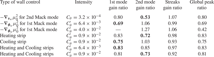
For blowing/suction control, we observe in figure 12(a) that the first Mack mode has also been reduced (optimal gain ratio of  $0.80$) because of the suction upstream. For 2-D disturbances, as seen in Appendix H, the second Mack mode is damped around the frequency where the gradient has been computed but increased at lower and higher frequencies, resulting in a shift of the second Mack mode to lower frequencies. Therefore, the overall optimal gain peak ratio of the second Mack mode is decreased to
 $0.53$, however, the blowing/suction mechanism is difficult to apply to realistic configurations.
Considering heat-flux control, in figure 12(b), the frequencies around the first Mack mode have been reduced, leading to an optimal gain ratio of  $0.69$. Nonetheless, as expected from the heat-flux gradients in figure 4(b), the second Mack mode is promoted by wall cooling, frequencies higher than
 $F=2.2 \times 10^{-4}$ being amplified. Increasing the intensity of the control (figure 12c) leads to the same results exhibiting a larger optimal gain for the second Mack mode while the first Mack mode is damped such that the local peak of this instability vanishes, making the streaks the most dominant mechanism (highest optimal gain).
In order to design a wall-control actuator which damps all instabilities, two avenues are revealed from the computations above (combining blowing and heating is not considered in this work). The first would be a series of suction actuators in the upstream part of the flat plate which would damp both Mack modes but this option is not selected because of practical implementation challenges in realistic configurations. The second is a series of constant heating and cooling strips with an appropriate location so that they would damp both Mack modes. By inspecting the heat-flux gradients in figure 4(b), the gradients for both Mack modes have the same direction in two locations: heating from the leading edge until  $Re_x=0.21 \times 10^6$ and cooling between
 $Re_x=1.045 \times 10^6$ and
 $Re_x=1.33 \times 10^6$. Therefore, we apply a constant heating strip at the first location and a constant cooling strip at the second location, the relative intensity of the heating/cooling strips being computed from the integrals (within each strip location) of the sum of the heat-flux gradients of both Mack modes, such that any of the mode is favoured. This yields to a similar amplitude for heating and cooling, the cooling being stronger by 1.175 than the heating.
We first study the effect of both strips independently and then together, at the same level of  $C_\theta '$. The temperature fields of the base flows are plotted in figure 13 and the resolvent gain maps in figure 14. First, for a single heating strip (figure 14a), two specific
 $F-\beta$ regions are damped: the first Mack mode/streak region and the second Mack mode region. There is also a region in the
 $F\unicode{x2013} \beta$ plane, where the instabilities are strengthened by the control, but the instabilities were weak initially in that region, so this actuator indeed attenuates all instabilities. Then, for a single cooling strip (figure 14b), instabilities for all wavenumbers and frequencies below
 $F=2.4 \times 10^{-4}$ are damped. Similarly to the cases where the full heat-flux gradient profile was prescribed at the wall, the second Mack mode is shifted to higher frequencies and amplified. Therefore, this actuator is very efficient to damp the first Mack mode but it is not robust enough to mitigate all the instabilities as a second Mack mode appearing at a larger frequency might be promoted by the cooling strip. Eventually, the control through a heating strip upstream and a cooling strip downstream (figure 14c) leads to a similar resolvent map and reduces by the same amount the optimal gains of both Mack modes than with a single heating strip. Moreover, the streaks are more damped with the additional cooling strip. Therefore, for the same energy spent, depending on the context, two strips may represent a better actuator as each strip requires the production of a smaller heat flux than a single heating strip but the mechanism would involve both a heating and a cooling strip.
Temperature of the controlled base flows. Solid line (respectively dashed) indicates the boundary layer thickness of the uncontrolled (respectively controlled) base flow. Dotted line (respectively dash-dotted) indicates the total energy deficit thickness  $\delta _E$ of the uncontrolled (respectively controlled) base flow. (a) Heating strip upstream with
 $C_\theta '=0.9 \times 10^{-2}$. (b) Cooling strip downstream with
 $C_\theta '=0.9 \times 10^{-2}$. (c) Heating strip upstream and cooling strip downstream with
 $C_\theta '=0.9 \times 10^{-2}$.

Optimal gain  $\mu _0$ of controlled boundary layers. White circle denotes the first Mack mode, black triangle denotes the streak mode and black square denotes the second Mack mode. Contour lines denote the ratio of the optimal gain with control over the optimal gain without control
 $\mu _0(C_\theta ' \neq 0)/\mu _0(C_\theta ' = 0)$ given by figure 3(a). (a) Heating strip upstream with
 $C_\theta '=0.9 \times 10^{-2}$. (b) Cooling strip downstream with
 $C_\theta '=0.9 \times 10^{-2}$. (c) Heating strip upstream and cooling strip downstream with
 $C_\theta '=0.9 \times 10^{-2}$.

To compare both types of control, a ratio of energy flux may be defined. However, since the induced mean skin-friction reduction cannot be inferred from the present linear analysis, it is not possible to interpret this ratio as an energetic efficiency (a full nonlinear analysis as in Rigas, Sipp & Colonius (Reference Rigas, Sipp and Colonius2021) needs to be conducted to evaluate the power saved due to the drag reduction with respect to the injected control power). Here, we compare, for both types of control, the ratio of the reduction of the outgoing disturbance energy flux, similarly to what was offered in the incompressible framework (Barbagallo et al. Reference Barbagallo, Dergham, Sipp, Schmid and Robinet2012; Sipp & Marquet Reference Sipp and Marquet2013), with the power provided at the wall. The flux of Chu's energy of the perturbations at the outlet of the optimisation domain  $\phi _{Chu} = \int _{x=x_{opt}} [\check {\boldsymbol {q}}(x,y)^* \boldsymbol {Q}_{Chu}(x,y)\check {\boldsymbol {q}}(x,y)] u(y) \, {\textrm {d}y}$ saved by the actuator is compared with the power consumed by the actuator. The ratios of power for heat-flux
 $\eta _{HC}$ and blowing/suction
 $\eta _{BS}$ control write
 $$\begin{gather} \eta_{HC} = (u'_{max})^{2} \frac{\Delta \phi}{\displaystyle\int\nolimits_{y=0} \lambda \left|\dfrac{\partial T}{\partial y}\right| {{\rm d}x} }, \end{gather}$$
 $$\begin{gather}\eta_{BS} = (u'_{max})^{2} \frac{\Delta \phi}{\displaystyle\int\nolimits_{y=0} \rho v^2 |v| \, {{\rm d}x}}, \end{gather}$$
where  $\Delta \phi =(\phi _{Chu}(C_\theta ' = 0 ) - \phi _{Chu}(C_\theta ' \neq 0))/\max {|\check {u}|^2}$ is the normalised reduction of disturbance energy flux, a constant that can be evaluated for given control efforts
 $C_\theta$ or
 $C_\theta '$ and a given spatial structure. Furthermore, the analysis being linear, we choose the amplitude of the disturbances by the maximal value
 $u'_{max}$ of the streamwise fluctuation velocity amplitude of the uncontrolled flow at the end of the optimisation domain. Considering the worst set of frequencies/spanwise wavenumbers given in table 2 and picking
 $u_{max}' = 0.01 U_\infty$ to remain within the linear regime, the heat-flux actuator power ratio is
 $\eta _{HC}=0.0029$ for the full gradient
 $-\boldsymbol {\nabla }_{\boldsymbol {\phi }_w} \mu _0^2$ at
 $C_\theta '=6.4 \times 10^{-3}$. For an actuator based on local strips, it decreases to
 $\eta _{HC} = 0.0010$ for a single heating strip (figure 14a) but only to
 $\eta _{HC} = 0.0019$ for two strips (figure 14c). For blowing/suction control, applying the full gradient
 $-\boldsymbol {\nabla }_{\boldsymbol {v}_w} \mu _0^2$ computed for the 2nd Mack mode at
 $C_\theta =3.2\times 10^{-4}$, the reduction of the global peak ratio is obtained with
 $\eta _{BS} = 348$. Therefore, a control based on the wall velocity mitigates better the fluctuations in comparison with wall-temperature control, however, the latter may be a better candidate for realistic applications.
To conclude, a relevant initial design for a wall actuator would be a thin steady heating strip located close to the leading edge (and possibly a second cooling strip downstream) which would modify the base flow so that the boundary layer is less receptive to streaks, first and second Mack modes. However, only linear computations were performed in this work. To properly design an optimal finite-amplitude actuator, one must perform a full iterative nonlinear evaluation (base-flow/stability/sensitivity analyses).
4. Conclusion
Optimal steady wall blowing and wall heating actuator locations for a Mach  $4.5$ boundary layer over an adiabatic flat plate have been calculated. Firstly, resolvent analyses have been performed around a base flow, highlighting the three main instabilities: the streaks, first and second Mack modes. An adjoint-based optimisation technique then allowed us to identify the optimal steady wall actuators to mitigate/strengthen the various instabilities.
Wall blowing/suction control induces streamwise momentum modifications in the corresponding sensitive region of the flow i.e. between the critical layer and the boundary layer thickness for both Mack modes. Wall heating/cooling control acts in the region of the flow sensitive to temperature variations for the first Mack mode i.e. within the boundary layer close to the wall but fails to induce temperature modifications above the critical layer where it is more optimal for the second Mack mode. For both Mack modes, the variations of optimal gain are driven by the streamwise momentum modifications always counterbalanced by the entropy modifications, except for the wall heat-flux control of the second Mack mode, where it is the entropy which promotes the optimal gain modification.
For steady wall blowing control, several conclusions are drawn. First, the second Mack mode is the most sensitive to blowing/suction control. Suction control is optimal to dampen the mode if located upstream of the synchronisation point and conversely for blowing control, in agreement with previous results found for roughness control. Secondly, the second Mack mode is optimally damped by a local suction device located in the region of branch I of the local mode  $S$ while the optimal region for the first Mack mode is around the maximum amplification rate of the local first mode. A steady blowing can damp the second Mack mode only if it is applied in the region of branch II of mode
 $S$. The application of the optimal wall suction and blowing control, computed for the second Mack mode, in the nonlinear regime (finite-amplitude control) yields a reduction of the optimal gain of the second Mack mode but shifts its peak to lower or higher frequencies, triggers a small decrease of the first Mack mode gains and leaves the streaks unaffected. Therefore, only a local suction actuator would efficiently dampen all instabilities.
The stability and sensitivity analyses have been repeated to find an optimal steady wall heat-flux actuator. The first Mack mode appears as the most sensitive instability to heating/cooling control. In agreement with previous findings (Mack Reference Mack1993), the first and second Mack modes have an opposite sensitivity with respect to wall-temperature changes, however, wall heating located close to the leading edge damps both Mack modes. In the downstream region, a large cooling region damps the first Mack mode while only a local cooling strip located in the unstable region of mode  $S$ damps the second Mack mode but this is suboptimal in comparison with the leading edge region. The application of the optimal wall heating and cooling control, computed for the first Mack mode, at a nonlinear regime yields a strong reduction of the first Mack mode gains but strongly amplifies the second Mack mode. The application of a single local steady heating strip close to the leading edge (and possibly a cooling strip downstream in the unstable region of mode
 $S$) manages to dampen all the instabilities and might be considered as an actuator to delay transition towards turbulence for a various range of frequencies and spanwise wavenumbers.
Funding
This work is funded by the French Agency for Innovation and Defence (AID) as part of the UK-FR PhD program. G.R. acknowledges funding from the Air Force Office of Scientific Research (AFOSR)/European Office of Aerospace Research and Development (EOARD) (award FA8655-21-1-7009). We are grateful to X. Chanteux for the share of his LST code.
Declaration of interests
The authors report no conflict of interest.
Appendix A. Chu's energy matrix
The Chu's energy (Chu Reference Chu1965) may be expressed into different forms depending on the set of variables used. For the following fluctuation variables: velocity  $\boldsymbol {\check {v}} = (\check {u}, \check {v}, \check {w})$, density
 $\check {\rho }$, pressure
 $\check {p}$, temperature
 $\check {T}$ and entropy
 $\check {s}$, Chu's energy writes, for instance, with dimensionless variables
 \begin{align} E_{Chu} = \boldsymbol{\check{q}}^* \boldsymbol{Q}_{Chu} \boldsymbol{\check{q}} & = \frac{1}{2} \int_\varOmega \left( \bar{\rho} \, \|\boldsymbol{\check{v}}\|^2 + \frac{1}{\gamma}\frac{\check{p}^2}{ \bar{p}} + \gamma (\gamma -1) M^4\, \bar{p}\, \check{s}^2 \right) {\rm d}\varOmega \nonumber\\ & = \frac{1}{2} \int_\varOmega \left( \bar{\rho} \, \|\boldsymbol{\check{v}}\|^2 + \frac{\bar{T}}{\bar{\rho}\gamma M^2} \, \check{\rho}^2 + \frac{\bar{\rho}}{(\gamma -1)\gamma M^2\bar{T}} \, \check{T}^2 \right) {\rm d}\varOmega, \end{align}
with  $\bar {q}$ indicating a base-flow variable. As the Navier–Stokes equations are written in conservative form with the state vector
 $\boldsymbol {q} = (\rho, \rho \boldsymbol {v}, \rho E)$, Chu's energy must be expressed with the conservative variables. For a spanwise homogeneous base flow (
 $\bar {w} = 0$), the disturbance variables defined around the base flow
 $\boldsymbol {\bar {q}}$ write
 $$\begin{gather} \check{u} = \frac{1}{\bar{\rho}}(\check{(\rho u)} - \bar{u} \check{\rho}), \end{gather}$$
 $$\begin{gather}\check{T} = \frac{(\gamma -1)\gamma M^2}{\bar{\rho}} \left[ \left( \frac{1}{2}(\bar{u}^2+\bar{v}^2) - \bar{e} \right) \check{\rho} - \bar{u} \check{(\rho u)} - \bar{v} \check{(\rho v)} + \check{(\rho E)} \right], \end{gather}$$
with  $\check {v}$ and
 $\check {w}$ defined similarly to
 $\check {u}$.
Following Bugeat et al. (Reference Bugeat, Chassaing, Robinet and Sagaut2019), two base-flow variables are introduced to simplify the notations
 $$\begin{gather} a_1 = \frac{(\gamma -1)\gamma M^2 \bar{\rho}}{\bar{T}}, \end{gather}$$
 $$\begin{gather}a_2 = \frac{\left(\dfrac{1}{2} (\bar{u}^2+\bar{v}^2) - \bar{e}\right)}{\bar{\rho}}. \end{gather}$$
Therefore, Chu's energy matrix writes in conservative form
 \begin{equation} \boldsymbol{Q}_{Chu} =
\frac{1}{2} \,{\rm d}\varOmega \left( \begin{array}{@{}ccccc@{}}
\dfrac{\bar{u}^2+\bar{v}^2}{\bar{\rho}} +
\dfrac{\bar{T}}{\bar{\rho} \gamma M^2} + a_1 a_2^2 & -
\dfrac{\bar{u}(1 + a_1 a_2)}{\bar{\rho}} & -
\dfrac{\bar{v}(1 + a_1 a_2)}{\bar{\rho}} & 0 & \dfrac{a_1
a_2}{\bar{\rho}} \\ -\dfrac{\bar{u}(1 +
a_1 a_2)}{\bar{\rho}} & \dfrac{1}{\bar{\rho}} +
\dfrac{\bar{u}^2 a_1 }{\bar{\rho}^2} & \dfrac{\bar{u}
\bar{v} a_1}{\bar{\rho}^2} & 0 & - \dfrac{\bar{u}
a_1}{\bar{\rho}^2} \\ -\dfrac{\bar{v}(1
+ a_1 a_2)}{\bar{\rho}} & \dfrac{\bar{u} \bar{v} a_1}{
\bar{\rho}^2} & \dfrac{1}{\bar{\rho}} + \dfrac{\bar{v}^2
a_1 }{\bar{\rho}^2} & 0 & - \dfrac{\bar{v}
a_1}{\bar{\rho}^2} \\ 0 & 0 & 0 &
\dfrac{1}{\bar{\rho}} & 0 \\ \dfrac{a_1
a_2}{\bar{\rho}} & -\dfrac{\bar{u} a_1}{\bar{\rho}^2} & -
\dfrac{\bar{v} a_1}{\bar{\rho}^2} & 0 &
\dfrac{a_1}{\bar{\rho}^2} \end{array} \right).
\end{equation}
Appendix B. Details of the sensitivity to base-flow modifications
The derivation of the sensitivity of the optimal gain to base-flow modifications is detailed
 \begin{align} \left\langle
\frac{\partial \mathcal{L}}{\partial \boldsymbol{\bar{q}}},
\delta \boldsymbol{\bar{q}} \right\rangle &= \left\langle
\boldsymbol{\lambda}_1, \mu_i \frac{\partial
(\boldsymbol{A} \boldsymbol{\check{q}}_i)} {\partial
\boldsymbol{q}} \delta \boldsymbol{\bar{q}} \right\rangle +
\Bigg\langle \boldsymbol{\lambda}_2 , \mu_i \frac{\partial
(\boldsymbol{Q}_q \boldsymbol{\check{q}}_i)}{\partial
\boldsymbol{q}} \delta \boldsymbol{\bar{q}} +
\frac{\partial (\boldsymbol{A^*}
\boldsymbol{\check{a}})}{\partial \boldsymbol{q}} \delta
\boldsymbol{\bar{q}}\Bigg\rangle - \Bigg\langle
\boldsymbol{\lambda}_3 , \mu_i^2 \frac{\partial
(\boldsymbol{Q}_f \boldsymbol{\check{f}}_i)}{\partial
\boldsymbol{q}} \delta \boldsymbol{\bar{q}} \Bigg\rangle
\nonumber\\
&= \left\langle \boldsymbol{\check{a}} , \mu_i
\frac{\partial (\boldsymbol{A}
\boldsymbol{\check{q}}_i)}{\partial \boldsymbol{q}} \delta
\boldsymbol{\bar{q}} \right\rangle + \Bigg\langle \mu_i
\boldsymbol{\check{q}}_i , \mu_i \frac{\partial
(\boldsymbol{Q}_q \boldsymbol{\check{q}}_i)}{\partial
\boldsymbol{q}} \delta \boldsymbol{\bar{q}} +
\frac{\partial (\boldsymbol{A^*}
\boldsymbol{\check{a}})}{\partial \boldsymbol{q}} \delta
\boldsymbol{\bar{q}}\Bigg\rangle - \Bigg\langle
\boldsymbol{\check{f}}_i , \mu_i^2 \frac{\partial
(\boldsymbol{Q}_f \boldsymbol{\check{f}}_i)}{\partial
\boldsymbol{q}} \delta \boldsymbol{\bar{q}} \Bigg\rangle
\nonumber\\
&= \mu_i \left\langle \left( \frac{\partial
(\boldsymbol{A} \boldsymbol{\check{q}}_i)}{\partial
\boldsymbol{q}} \right)^* \boldsymbol{\check{a}} , \delta
\boldsymbol{\bar{q}} \right\rangle + \mu_i \left\langle
\left( \frac{\partial (\boldsymbol{A}^*
\boldsymbol{\check{a}})}{\partial \boldsymbol{q}} \right)^*
\boldsymbol{\check{q}}_i, \delta
\boldsymbol{\bar{q}}\right\rangle \nonumber\\
&\quad + \mu_i^2 \Bigg\langle \Bigg( \frac{\partial
(\boldsymbol{Q}_q \boldsymbol{\check{q}}_i)}{\partial
\boldsymbol{q}} \Bigg)^* \boldsymbol{\check{q}}_i, \delta
\boldsymbol{\bar{q}}\Bigg\rangle - \mu_i^2 \Bigg\langle
\Bigg( \frac{\partial (\boldsymbol{Q}_f
\boldsymbol{\check{f}}_i)}{\partial \boldsymbol{q}}
\Bigg)^* \boldsymbol{\check{f}}_i , \delta
\boldsymbol{\bar{q}} \Bigg\rangle.
\end{align}
By writing the operators in component notations, one can find that
 \begin{equation} \left(\frac{\partial (\boldsymbol{A}^* \boldsymbol{\check{a}})}{\partial \boldsymbol{q}} \right)^* \boldsymbol{\check{q}}_i = \boldsymbol{\check{a}}^* \left( \frac{\partial (\boldsymbol{A} \boldsymbol{\check{q}}_i)}{\partial \boldsymbol{q}} \right), \end{equation}
and therefore the sum of both complex conjugates gives rise to twice the real part
 \begin{align} \Bigg\langle
\frac{\partial \mathcal{L}}{\partial \boldsymbol{\bar{q}}},
\delta \boldsymbol{\bar{q}} \Bigg\rangle &= \Bigg\langle
2\mu_i \,{\rm Re}\Bigg(\Bigg( \frac{\partial
(\boldsymbol{A} \boldsymbol{\check{q}}_i)}{\partial
\boldsymbol{q}} \Bigg)^* \boldsymbol{\check{a}} \Bigg) +
\mu_i^2 \Bigg( \frac{\partial (\boldsymbol{Q}_q
\boldsymbol{\check{q}}_i)}{\partial \boldsymbol{q}}
\Bigg)^* \boldsymbol{\check{q}}_i \nonumber\\
&\quad - \mu_i^2 \Bigg( \frac{\partial
(\boldsymbol{Q}_f \boldsymbol{\check{f}}_i)}{\partial
\boldsymbol{q}} \Bigg)^* \boldsymbol{\check{f}}_i , \delta
\boldsymbol{\bar{q}} \Bigg\rangle,
\end{align}
and getting from (2.15a–c) that  $\mu _i \boldsymbol {Q}_q \boldsymbol {\check {q}}_i = \boldsymbol {\mathcal {R}}^{-1*} \boldsymbol {\check {a}}$, one has
 \begin{align} \Bigg\langle
\frac{\partial \mathcal{L}}{\partial \boldsymbol{\bar{q}}},
\delta \boldsymbol{\bar{q}} \Bigg\rangle &= \Bigg\langle
2\mu_i^2\,{\rm Re}\Bigg(\Bigg( \frac{\partial
(\boldsymbol{A} \boldsymbol{\check{q}}_i)}{\partial
\boldsymbol{q}} \Bigg)^* \boldsymbol{\mathcal{R}}^{*}
\boldsymbol{Q}_q \boldsymbol{\check{q}}_i \Bigg) + \mu_i^2
\Bigg( \frac{\partial (\boldsymbol{Q}_q
\boldsymbol{\check{q}}_i)}{\partial \boldsymbol{q}}
\Bigg)^* \boldsymbol{\check{q}}_i \nonumber\\
&\quad - \mu_i^2 \Bigg( \frac{\partial
(\boldsymbol{Q}_f \boldsymbol{\check{f}}_i)}{\partial
\boldsymbol{q}} \Bigg)^* \boldsymbol{\check{f}}_i, \delta
\boldsymbol{\bar{q}} \Bigg\rangle, \nonumber\\
\Rightarrow \boldsymbol{\nabla}_{\boldsymbol{\bar{q}}} \mu_i ^2 &=
2\mu_i^2\,{\rm Re}\big( \boldsymbol{H}'^*
\boldsymbol{\mathcal{R}}^{*} \boldsymbol{Q}_q
\boldsymbol{\check{q}}_i \big) + \mu_i^2 \Bigg(
\frac{\partial (\boldsymbol{Q}_q
\boldsymbol{\check{q}}_i)}{\partial \boldsymbol{q}}
\Bigg)^* \boldsymbol{\check{q}}_i - \mu_i^2 \Bigg(
\frac{\partial (\boldsymbol{Q}_f
\boldsymbol{\check{f}}_i)}{\partial \boldsymbol{q}}
\Bigg)^* \boldsymbol{\check{f}}_i,
\end{align}
where  $\operatorname {Re}({\cdot })$ is the real part. Expressing the sparse Hessian operator
 $\boldsymbol {H}$ as
 \begin{equation} H_{ijk} = \left. \frac{\partial^2 R_i}{\partial q_j \partial q_k} \right|_{\boldsymbol{\bar{q}}}, \end{equation}
we get that  $\boldsymbol {H}(\boldsymbol {\check {q}}, \delta \boldsymbol {\bar {q}}) = ({\partial ( \boldsymbol {A} \boldsymbol {\check {q}} )}/{\partial \boldsymbol {q}} )\delta \boldsymbol {\bar {q}}$. We can then define the matrix
 $\boldsymbol {H}'$ as
 $\boldsymbol {H}' \delta \boldsymbol {\bar {q}}= \boldsymbol {H}(\boldsymbol {\check {q}}, \delta \boldsymbol {\bar {q}})$ and then equation (B4) gives the sensitivity of the optimal gain to base-flow modifications (2.19).
Appendix C. Sensitivity to momentum-divergence-free base-flow modifications
From the sensitivity to base-flow modifications  $\boldsymbol {\nabla }_{\boldsymbol {\bar {q}}} \mu _i^2$ given by (2.19), a restriction to momentum-divergence-free base-flow variations can be performed. Denoting
 $\boldsymbol {\nabla }_{\boldsymbol {\bar {\rho u}}}^{df} \mu _i^2$ and
 $\boldsymbol {\nabla }_{\boldsymbol {\bar {\rho v}}}^{df} \mu _i^2$ the sensitivities to momentum-divergence-free modifications of the base-flow momentum, any momentum-divergence-free base-flow modifications
 $\delta ^{df} \bar {\boldsymbol {\rho u}}$ and
 $\delta ^{df} \bar {\boldsymbol {\rho v}}$ yield
 \begin{equation} \delta \mu_i^2 = \langle \boldsymbol{\nabla}_{\boldsymbol{\bar{\rho u}}}^{df} \mu_i^2, \delta^{df} \bar{\boldsymbol{\rho u}} \rangle + \langle \boldsymbol{\nabla}_{\boldsymbol{\bar{\rho v}}}^{df} \mu_i^2, \delta^{df} \bar{\boldsymbol{\rho v}} \rangle = \langle \boldsymbol{\nabla}_{\boldsymbol{\bar{\rho u}}} \mu_i^2, \delta^{df} \bar{\boldsymbol{\rho u}} \rangle + \langle \boldsymbol{\nabla}_{\boldsymbol{\bar{\rho v}}} \mu_i^2, \delta^{df} \bar{\boldsymbol{\rho v}} \rangle. \end{equation}
As the sensitivity and the momentum base-flow modifications are both momentum- divergence free, they can be written as functions of scalars
 \begin{equation} \boldsymbol{\nabla}_{\boldsymbol{\bar{\rho u}}}^{df} \mu_i^2 = \frac{\partial \psi}{\partial y}, \quad \boldsymbol{\nabla}_{\boldsymbol{\bar{\rho v}}}^{df} \mu_i^2 =-\frac{\partial \psi}{\partial x}, \quad \delta^{df} \bar{\boldsymbol{\rho u}} = \frac{\partial \phi}{\partial y}, \quad \delta^{df} \bar{\boldsymbol{\rho v}} =- \frac{\partial \phi}{\partial x}. \end{equation}
Injecting (C2a–d) into (C1) and assuming that the equation should be valid for any scalar  $\phi$, an integration by parts leads to the Poisson equation
 \begin{equation} -\Delta \psi = \frac{\partial \boldsymbol{\nabla}_{\boldsymbol{\bar{\rho v}}} \mu_i^2}{\partial x} - \frac{\partial \boldsymbol{\nabla}_{\boldsymbol{\bar{\rho u}}} \mu_i^2}{\partial y}, \end{equation}
with the boundary conditions  $\boldsymbol {\nabla } \psi \boldsymbol {\cdot } \boldsymbol {n} = n_y \boldsymbol {\nabla }_{\boldsymbol {\bar {\rho u}}} \mu _i^2 - n_x \boldsymbol {\nabla }_{\boldsymbol {\bar {\rho v}}} \mu _i^2$ and
 $\boldsymbol {n} = (n_x,n_y)$ the boundary normal.
Appendix D. Wall-boundary condition for blowing and heat flux
The implementation of the boundary conditions in the code BROADCAST is described in further details in Poulain et al. (Reference Poulain, Content, Sipp, Rigas and Garnier2023). They are enforced through the addition of ghost cells to prescribe characteristic-based conditions for permeable boundaries or mixed Dirichlet–Neumann conditions for solid boundaries. The wall-boundary conditions with non-zero heat flux and wall-normal velocity is derived below as they play a major role in the computation of the sensitivity.
The boundary layer assumption is performed involving a zero pressure gradient in the wall-normal direction:  $\partial p/\partial n=0$ with
 $n$ the wall-normal direction. From the derivative in the wall-normal direction of the perfect gas law (2.5), computed at the wall, one gets
 \begin{equation} \left. \frac{\partial p}{\partial n} \right|_w = \rho_w r \left. \frac{\partial T}{\partial n}\right|_w + r T_w \left.\frac{\partial \rho}{\partial n}\right|_w, \end{equation}
with the subscript  ${\cdot }_w$ indicating the values at the wall. The temperature
 $T_w$ is replaced by
 $p_w/(\rho _w r)$ from the perfect gas law. The pressure at the wall
 $p_w$ is known from the value in the first cell as
 $\partial p/\partial n=0$ and the temperature gradient writes as a heat flux
 $\phi =\lambda \partial T/\partial n$. Therefore, assuming a first-order extrapolation for the density, (D1) becomes a function of a single unknown, the wall density
 $\rho _w$
 \begin{equation} -\frac{r}{2 \lambda p_w} \phi_w \rho_w^2 + \rho_w - \rho_1 = 0, \end{equation}
with  $\rho _1$ the density at the first cell centre. For an adiabatic wall condition
 $\phi _w=0$, we get
 $\rho _w=\rho _1$, otherwise we obtain
 $\rho _w = (1-\sqrt {1-2r\phi _w \rho _1/(\lambda p_w)})/(r\phi _w /(\lambda p_w))$. However, the latter expression for
 $\rho _w$ is not differentiable around
 $\phi _w=0$. Then, in order to compute the Jacobian and Hessian of an adiabatic flow, which respectively involve the first and second derivatives of the wall-boundary conditions, (D2) is solved by a Newton method to compute
 $\rho _w$, this iterative method being then linearised by AD to build the derivative operators. Eventually, all the conservative variables are prescribed at the wall:
 $\rho _w$,
 $(\rho u)_w = 0$ (no-slip),
 $(\rho v)_w = \rho _w \times v_w$ (with a non-zero
 $v_w$ for a wall-normal blowing/suction condition) and
 $(\rho E)_w = p_w/(\gamma -1) + 0.5 \rho _w v_w^2$.
Appendix E. Validation on a low Mach number boundary layer
The discrete linear sensitivity of the optimal gain to steady blowing is validated on an adiabatic flat plate in the low Mach number regime against Brandt et al. (Reference Brandt, Sipp, Pralits and Marquet2011) where the sensitivity analysis had been derived in a continuous and incompressible framework.
The free-stream Mach number is  $M=0.1$, the Reynolds number is
 $Re=6 \times 10^5$. The computational domain extends from
 $Re_{x,{in}} = 4300$ to
 $Re_{x,{out}} = 7.5 \times 10^5$, the optimisation for the resolvent mode is restrained up to
 $Re_x \leqslant 6 \times 10^5$ inside
 $\boldsymbol {Q}_q$ and
 $\boldsymbol {P}$. The height of the domain is about
 $9\,\delta$ with
 $\delta$ the displacement thickness at
 $Re_x = 6 \times 10^5$. The following boundary conditions are applied: Blasius solution prescribed at the inlet (non-reflecting subsonic), adiabatic no-slip wall at the bottom, non-reflecting condition at the top and non-reflecting subsonic condition at the outlet with the free-stream pressure taken as reference (zero pressure gradient assumed). A Cartesian mesh similar to the supersonic boundary layer case is chosen with
 $(N_x, N_y) = (1000, 150)$.
In Brandt et al. (Reference Brandt, Sipp, Pralits and Marquet2011), the largest optimal gain at zero frequency is obtained for the streaks at  $\beta \delta = 0.94$. The sensitivity of this 3-D mode to steady wall blowing is plotted in figure 15. They show good agreement while we compare two different frameworks: discrete linearisation in a low Mach compressible framework in our work while Brandt et al. (Reference Brandt, Sipp, Pralits and Marquet2011) used a continuous linearisation in the incompressible framework. However, slight discrepancies are noticed in the leading edge part, which can be explained by the fact that the leading edge was included inside the computational domain used in Brandt et al. (Reference Brandt, Sipp, Pralits and Marquet2011) while we start at
 $Re_{x,{in}} = 4300$.
Normalised sensitivity of the optimal gain of the streaks ( $\beta \delta = 0.94$) to wall blowing
 $\boldsymbol {\nabla }_{\boldsymbol {v}_w} \mu ^2$. Comparison with Brandt et al. (Reference Brandt, Sipp, Pralits and Marquet2011).

Appendix F. Local stability analysis
In this study, local stability analysis is applied only to characterise the gradients given by the sensitivity of the optimal gains but is never required to perform the sensitivity analysis itself.
Linear LST is valid only on parallel flows in the streamwise direction. Under this assumption, an ansatz of the fluctuations is made of the form
 \begin{equation} \boldsymbol{q}' = \boldsymbol{\hat{q}}(y) \exp({{\rm i}(\alpha x - \omega t+ \beta z)}). \end{equation}
For the spatial LST (Schmid, Henningson & Jankowski Reference Schmid, Henningson and Jankowski2002), the frequency  $\omega$ is set real (
 $\omega = \omega _r$) and the streamwise wavenumber
 $\alpha$ is complex (
 $\alpha = \alpha _r + \textrm {i} \alpha _i$). Linearising the Navier–Stokes equations and injecting (F1) leads to a dispersion relation between
 $\alpha$,
 $\omega$,
 $Re_x$ and
 $M$. Fixing the three latter parameters, the dispersion relation gives the complex value of
 $\alpha$. Depending on the sign of
 $\alpha _i$, the disturbances exponentially decay (
 $\alpha _i>0$) or grow (
 $\alpha _i<0$) in the streamwise direction. The phase velocity
 $c$ is defined as
 \begin{equation} c = c_r + {\rm i} c_i = \frac{\omega}{\alpha} = \frac{\omega_r \alpha_r}{|\alpha|^2} - {\rm i} \frac{\omega_r \alpha_i}{|\alpha|^2}. \end{equation}
The linear LST numerical method relies on a Chebyshev collocation method for the wall-normal direction and the dispersion relation is solved through LAPACK library. An isothermal boundary condition is prescribed for the linearised disturbances ( $T'=0$ at wall). The code has been developed by Chanteux et al. (Reference Chanteux, Bégou, Deniau and Vermeersch2022) following the Saint-James (Reference Saint-James2020) framework and validated on a supersonic boundary layer by Nibourel et al. (Reference Nibourel, Leclercq, Demourant, Garnier and Sipp2023).
Appendix G. Sensitivity to base-flow modifications and steady forcing
The sensitivities of the optimal gain of the first and second Mack modes to base-flow modifications  $\boldsymbol {\nabla }_{\boldsymbol {\bar {q}}} \mu _ 0^2$ are computed. To highlight the most predominant contributions in the sensitivity, the total optimal gain variation has been split (2.29) into base-flow variation components of streamwise kinetic energy
 $\delta E_{k_x}^b$, wall-normal kinetic energy
 $\delta E_{k_y}^b$, pressure
 $\delta E_{p}^b$ and entropy
 $\delta E_{s}^b$. These quantities have been reported in figure 16. The largest component for both Mack modes seems to be the wall-normal kinetic energy. However, as noticed in previous studies (Brandt et al. Reference Brandt, Sipp, Pralits and Marquet2011; Park & Zaki Reference Park and Zaki2019), a strong wall-normal base-flow velocity modification is not physical since base-flow momentum fields are momentum-divergence free (
 ${\partial _x \delta \boldsymbol {\bar {\rho u}}} + {\partial _y \delta \boldsymbol {\bar {\rho v}}}= 0$). The addition of this constraint strongly damps the wall-normal velocity component of the sensitivity. Therefore, the largest component of the sensitivity becomes the streamwise velocity for both Mack modes followed by the entropy
 $\delta E_s^b$ and pressure
 $\delta E_p^b$ components, which are one order of magnitude lower for both Mack modes. Overall, the second Mack mode is more sensitive than the first Mack mode. The same conclusions are drawn for the streaks with a sensitivity much below the first Mack mode.
Normalised Chu energy norm components of the sensitivity to base-flow modifications  $\boldsymbol {\nabla }_{\bar {\boldsymbol {q}}} \mu _0^2 /\mu _0^2$ (first bar), to momentum-divergence-free base-flow modifications
 $\boldsymbol {\nabla }_{\bar {\boldsymbol {q}}}^{df} \mu _0^2 /\mu _0^2$ (second bar) and to steady forcing
 $\boldsymbol{\nabla}_{\!\bar {\boldsymbol {f}}} \mu _0^2 /\mu _0^2$ (third bar).

In figure 17(a,c), the sensitivity to local modifications of the streamwise base-flow momentum  $\boldsymbol {\nabla }_{\overline {\boldsymbol {{\rho u}}}} \mu _0^2$ is plotted for both Mack modes. The sensitivity of the first Mack mode extends longer in the streamwise direction than the second Mack mode, as expected from the wavemaker support (overlap of optimal forcing and response from the resolvent analysis). These sensitivities are strongest in the region between the displacement thickness
 $\delta ^*$ and the boundary layer thickness
 $\delta _{99}$ (
 $u(y=\delta _{99}) = 0.99 U_\infty$). This recalls the local results found for Fedorov's mode
 $S$ (Park & Zaki Reference Park and Zaki2019) or for the incompressible T–S waves (Brandt et al. Reference Brandt, Sipp, Pralits and Marquet2011), the sensitivities
 $\boldsymbol {\nabla }_{\overline {\boldsymbol {{\rho u}}}} \mu _0^2$ of the first and second Mack modes being negative at the critical layer
 $y_c$ (McKeon & Sharma Reference McKeon and Sharma2010) (
 $u(y_c)=c_r$ with
 $c_r=Re(\omega /\alpha )$ the phase velocity of the mode) and positive in the vicinity above and below. Park & Zaki (Reference Park and Zaki2019) and Guo et al. (Reference Guo, Gao, Jiang and Lee2021) showed that the mean shear modification contributes the most to the sensitivity resulting in a receptive region around the critical layer. Besides, from figure 17(c), it is seen that, for the second Mack mode, the generalised inflection line
 $y_{GIP}$ (
 $\partial [\rho \partial u/\partial y]/\partial y(y_{GIP}) = 0$) of the base flow, where the optimal forcing and optimal entropy response are maximal, is close to the critical layer
 $y_c$ of the optimal response.
Linear sensitivity of the optimal gain to base-flow modifications  $\boldsymbol {\nabla }_{\bar {\boldsymbol {q}}} \mu _0^2 /\mu _0^2$. Solid line represents the boundary layer thickness, dash-dotted line indicates the generalised inflection point, dashed line is the displacement thickness and dotted line is the critical layer. (a,b) Sensitivity of the first Mack mode.(c,d) Sensitivity of the second Mack mode. (a,c) Streamwise component of the momentum
 $\boldsymbol {\nabla }_{\overline {\boldsymbol {{\rho u}}}} \mu _0^2 /\mu _0^2$ (similar to the momentum-divergence-free component). (b,d) Temperature component
 $\boldsymbol {\nabla }_{\bar {\boldsymbol {T}}} \mu _0^2 /\mu _0^2$.

In figure 17(b,d), the sensitivity to local modifications of the base-flow temperature  $\boldsymbol {\nabla }_{\bar {\boldsymbol {T}}} \mu _0^2$ is plotted for both Mack modes. The gradient
 $\boldsymbol {\nabla }_{\bar {\boldsymbol {T}}} \mu _0^2$ is computed from the components of
 $\boldsymbol {\nabla }_{\bar {\boldsymbol {q}}} \mu _0^2$ through the linearisation of the definition of the total energy
 $E$ (chain rule)
 \begin{align} \boldsymbol{\nabla}_{\bar{\boldsymbol{T}}} \mu_0^2 = \frac{(\gamma -1)\gamma M^2}{\bar{\rho}} \left( \left( \frac{1}{2} (\bar{u}^2 + \bar{v}^2) - \bar{e} \right) \boldsymbol{\nabla}_{\bar{\boldsymbol{\rho}}} \mu_0^2 - \bar{u} \boldsymbol{\nabla}_{\overline{\boldsymbol{{\rho u}}}} \mu_0^2 - \bar{v} \boldsymbol{\nabla}_{\overline{\boldsymbol{{\rho v}}}} \mu_0^2 + \boldsymbol{\nabla}_{\bar{\boldsymbol{\rho E}}} \mu_0^2 \right). \end{align}
The gradient  $\boldsymbol {\nabla }_{\bar {\boldsymbol {T}}} \mu _0^2$ is not solely located between
 $y_c$ and
 $\delta _{99}$ anymore. A strong region of the gradient also exists closer to the wall for both Mack modes. In the case of the first Mack mode, the critical layer
 $y_{c}$ line separates a positive (
 $y< y_{c}$) and a negative (
 $y>y_{c}$) region of the gradient, likely resulting once again from the mean shear distortion. For the second Mack mode, although the sensitivity
 $\boldsymbol {\nabla }_{\bar {\boldsymbol {T}}} \mu _0^2$ is similar to
 $\boldsymbol {\nabla }_{\overline {\boldsymbol {{\rho u}}}} \mu _0^2$, there is an additional region of large sensitivity to changes of the base-flow temperature close to the wall from
 $Re_x=10^6$ until the end of the domain.
From the sensitivity to base-flow modifications  $\boldsymbol {\nabla }_{\bar {\boldsymbol {q}}} \mu _0^2$, the sensitivity of the optimal gain to a steady volume forcing term
 $\boldsymbol {\nabla }_{\bar {\boldsymbol {f}}} \mu _0^2$ is deduced. Chu's energy norm of the sensitivity
 $\boldsymbol {\nabla }_{\bar {\boldsymbol {f}}} \mu _0^2$, as well as its decomposition into different components, is reported in figure 16. The different contributions reflect those of the momentum-divergence-free base-flow gradient
 $\boldsymbol {\nabla }_{\bar {\boldsymbol {q}}}^{df} \mu _0^2$ for both Mack modes, however, the components induced by base-flow pressure variations are larger than those induced by entropy variations and their sum
 $\delta E_p^b + \delta E_s^b$ exhibits a magnitude similar to the streamwise kinetic energy component
 $\delta E_{k_x}^b$. For the streaks, the pressure component
 $\delta E_{p}^b$ is equivalent to the streamwise kinetic energy component
 $\delta E_{k_x}^b$ while its entropy component
 $\delta E_{s}^b$ is much smaller. The three instabilities display a sensitivity of similar magnitude.
In figure 18(a,c), the sensitivity to a steady streamwise momentum source term  $\boldsymbol {\nabla }_{\overline {\boldsymbol {f_{\rho u}}}} \mu _0^2$ is plotted for both Mack modes. The gradients for both Mack modes are very similar with a positive region around the boundary layer thickness
 $\delta _{99}$ and a negative region around the displacement thickness
 $\delta ^*$. The mechanism below this gradient might be the local thickening of the boundary layer by the increase of the streamwise mean velocity above the edge and its decrease below.
Linear sensitivity of the optimal gain to steady forcing  $\boldsymbol{\nabla}_{\!\bar {\boldsymbol {f}}} \mu _0^2 /\mu _0^2$. Solid line represents the boundary layer thickness, dash-dotted line indicates the generalised inflection point, dashed line is the displacement thickness and dotted line is the critical layer. (a,b) Sensitivity of the first Mack mode.(c,d) Sensitivity of the second Mack mode. (a,c) Streamwise component of the momentum
 $\boldsymbol {\nabla }_{\overline {\boldsymbol {f_{\rho u}}}} \mu _0^2 /\mu _0^2$. (b,d) Temperature component
 $\boldsymbol {\nabla }_{\overline {\boldsymbol {f_{T}}}} \mu _0^2 /\mu _0^2$.

Then, the sensitivity to a steady heating source term  $\boldsymbol {\nabla }_{\overline {\boldsymbol {f_{T}}}} \mu _0^2$, computed with (G1) by replacing the components of
 $\boldsymbol {\nabla }_{\bar {{\boldsymbol {q}}}} \mu _0^2$ by
 $\boldsymbol {\nabla }_{\bar {\boldsymbol {f}}} \mu _0^2$, is plotted in figure 18(b,d) for both Mack modes. As for
 $\boldsymbol {\nabla }_{\bar {\boldsymbol {T}}} \mu _0^2$, the sensitivity
 $\boldsymbol {\nabla }_{\overline {\boldsymbol {f_{T}}}} \mu _0^2$ has strong distortions inside the boundary layer. For the first Mack mode, the gradient is mainly positive from the wall up to the critical layer (
 $y< y_c$) except in the region close to the leading edge. However, in the case of the second Mack mode, the largest region of sensitivity (negative gradient) is between the displacement thickness and the boundary layer thickness. Inside the boundary layer, closer to the wall, the gradient varies a lot in the streamwise direction for the second Mack mode. From an overall perspective, a steady heating source term has an opposite effect inside the boundary layer between the first and the second Mack modes. This recalls the well-known effect of stabilisation by cooling for the first Mack mode and by heating for the second Mack mode (Mack Reference Mack1993).
Appendix H. Sensitivity of the second Mack mode to steady wall blowing
The sensitivity analysis and all the subsequent steps performed for the steady wall heating control are repeated in the case of the steady wall blowing/suction control. The optimal steady wall-normal velocity profile to damp the second Mack mode and its decomposition into various components are plotted in figure 19. As seen from the integral energy in figure 7, the gradient  $\boldsymbol {\nabla }_{\boldsymbol {v}_w}\mu _0^2$ is mainly produced from the sensitivity term due to the base-flow variation as the term due to the Jacobian variation is of smaller amplitude. The low impact of the Jacobian modifications on the gradient is due to the fact that the wall-normal velocity prescribed at the wall only appears in the energy equation in the linearised wall-boundary condition.
Optimal wall-velocity profile to damp the second Mack mode i.e. opposite of the sensitivity of the optimal gain of the second Mack mode to wall blowing  $-\delta \boldsymbol {p}^{m} = - \delta \boldsymbol {v}_w$. Base-flow component
 $- \delta \boldsymbol {p}_{\bar {\boldsymbol {q}}}^m$ and Jacobian component
 $-\delta \boldsymbol {p}_{\boldsymbol {A}}^m$ are also indicated, the latter being almost zero.

The total gradient may be split into two main parts: suction in the upstream region up to  $Re_x \approx 1.2 \times 10^6$ and blowing downstream. The same behaviour is noticed at a different frequency (see Appendix I).
In the following, to fix the control amplitude, similarly to the energy coefficient  $C_\theta '$, we introduce the momentum coefficient
 $C_\theta$ as the ratio between the momentum injected at the wall and the free-stream momentum deficit
 \begin{equation} C_\theta = \frac{ \displaystyle\int\nolimits_{y=0} |(\rho v^2)'| \,{{\rm d}x}}{ \displaystyle\int\nolimits_{x=x_{out}} (\rho_\infty U_\infty^2 - \rho u^2)\,{{\rm d}y} }, \end{equation}
with  $(\rho v^2)'$ the difference of wall-normal momentum
 $\rho v^2$ between controlled and uncontrolled base flows. To understand the effect of the control profile shown in figure 19, we compare local stability (spatial LST) analysis results applied to the uncontrolled base flow and to the controlled base flow with the full stabilising gradient at
 $C_\theta = 3.2 \times 10^{-6}$. Fong et al. (Reference Fong, Wang and Zhong2014) indeed showed that the location of a roughness element upstream or downstream the synchronisation point results in opposite stabilisation effects. We find similar trends as the intersection of the phase velocities of Fedorov's modes
 $F$ and
 $S$ is close to the point where the gradient is null in figure 19. We also highlight that the locations of branch I and branch II of mode S are respectively close to the maxima for suction and for blowing.
Phase velocities and amplification rates of modes  $S$ and
 $F$ are shown in figure 20 with and without the application of the stabilising wall profile. Unlike the heating/cooling case, the phase velocity of mode
 $S$ remains quite similar in both cases while the phase velocity of mode
 $F$ of the controlled base flow slightly deviates from the original in the control region. This results in a shorter synchronisation region between modes
 $F$ and
 $S$, leading to a shorter unstable region for the amplification rate of mode
 $S$ only induced by the modification of branch I location. Zhao et al. (Reference Zhao, Wen, Tian, Long and Yuan2018) noticed the same behaviour for the phase velocity in the case of heating and cooling strip control.
Local stability analysis of an uncontrolled base flow (solid lines) and a controlled base flow (dashed lines) with the optimal wall-velocity profile  $-\boldsymbol {\nabla }_{\boldsymbol {v}_w} \mu _0^2 /\mu _0^2$ at
 $C_\theta = 3.2 \times 10^{-6}$. (a) Phase velocity
 $c_r/U_\infty$. Dashed lines denote from top to bottom the phase velocities
 $1 + 1/M_\infty$,
 $1$ and
 $1-1/M_\infty$. (b) Amplification rate
 $\alpha _i \delta ^*$.

In the following, we compare the prediction obtained by the gradient approach and the exact results obtained by computing the modified base flow and the associated resolvent gains.
We plot in figure 21(a) the optimal gain variations for  $\beta =0$ as a function of frequency
 $F$. The maximal optimal gain reduction for different values of
 $C_\theta$ is reported in table 3. At
 $C_\theta = 3.2 \times 10^{-8}$, the linear prediction remains accurate while from
 $C_\theta = 3.2 \times 10^{-6}$, the nonlinear (
 $0.811$) and linear (
 $0.686$) predicted optimal gain ratios of the second Mack mode deviate from each other (the 2-D first Mack mode being well predicted by the linear sensitivity according to figure 21a). Increasing further the blowing momentum coefficient
 $C_\theta$ allows reaching of an optimal gain ratio of
 $0.62$ at
 $C_\theta = 1.2 \times 10^{-4}$. However, we observe from the curve
 $\mu (F)$ in figure 21(a) that the control damps efficiently the optimal gain at the frequency where it was computed but not for lower or higher frequencies, resulting in a split of the second Mack mode into two peak regions: a first peak at
 $F=2 \times 10^{-4}$ and a second for higher frequencies above
 $F=3 \times 10^{-4}$. This effect was also noticed by Miró Miró & Pinna (Reference Miró Miró and Pinna2018) on the growth rate. The optimisation procedure could in principle be pursued by computing a new descend direction to eventually reach a local/global minimum.
Resolvent analysis for different base flows controlled with the optimal wall-velocity profile  $-\boldsymbol {\nabla }_{\boldsymbol {v}_w} \mu _0^2 /\mu _0^2$. (a) Optimal gain
 $\mu$ for
 $\beta =0$ with respect to the frequency
 $F$ for
 $C_\theta =0$ (blue),
 $C_\theta =3.2 \times 10^{-6}$ (red),
 $C_\theta =1.3 \times 10^{-5}$ (yellow),
 $C_\theta =1.2 \times 10^{-4}$ (green) and
 $C_\theta =3.2 \times 10^{-4}$ (orange). Solid lines indicate the optimal gain
 $\mu _0$ while dashed lines indicate the first suboptimal gain
 $\mu _1$. The stars indicate the linear gain predicted from the gradient. (b) Energy density
 $d_{Chu}$ of the optimal forcing (dashed lines) and response (solid lines) of the second Mack mode without control (green) and for the controlled base flow at
 $C_\theta =3.2 \times 10^{-6}$ (red). Black vertical line indicates the end of the optimisation domain for resolvent analysis.

Optimal gain evolution of the second Mack mode with respect to the optimal wall-velocity profile  $-\boldsymbol {\nabla }_{\boldsymbol {v}_w} \mu _0^2 /\mu _0^2$ at various momentum coefficient
 $C_\theta$ intensities. Gain ratio is computed by
 ${\mu _0(C_\theta \neq 0)/\mu _0(C_\theta = 0)}$. The expected linear gain ratio is computed by
 $\sqrt {\mu _0^2- \epsilon \|\boldsymbol {\nabla }_{\boldsymbol {p}} \mu _0^2 \|^2}/\mu _0$ with
 $\epsilon$ being a function of
 $C_\theta$. The X indicates that the linear gain ratio would predict a negative value.

Figure 21(a) overall shows that the control applied to the base flow strongly reduces the optimal gain  $\mu _0$ for the initial frequency of the second Mack mode without modifying the gains of the sub-optimal gain
 $\mu _1$. While the optimal gain is effectively damped with an increased wall-normal velocity control, the sub-optimal gain remains of similar magnitude compared with the no-control case and does not increase. This results in a low-rankness loss of the system (ratio of approximately 4 between optimal and suboptimal gains which decreases to 2 for
 $C_\theta = 1.2 \times 10^{-4}$). Therefore, as for heating/cooling control, for larger control intensity, the optimal gain alone is not sufficient anymore to characterise the linear dynamics of the boundary layer.
Chu's energy densities of the optimal forcing and response with blowing/suction control at  $C_\theta = 3.2 \times 10^{-6}$ are plotted in figure 21(b) and compared with the results without control. The optimal forcing has been shifted slightly downstream while the optimal response exhibits a slightly smaller support. The downstream shift of the optimal forcing is expected as the boundary layer thickness has been locally reduced because of the suction at the wall until
 $Re_x = 1.2 \times 10^6$. The response is not shifted downstream as the wall blowing control increases again the boundary layer thickness to almost recover its value without control (an example of boundary layer thicknesses with and without control is shown in figure 11a). This can be understood from spatial LST results, where branch I is shifted downstream while branch II does not move.
Appendix I. Gradient dependence with frequency
To check how the gradients evolve with the instability frequency, 2-D stability and sensitivity are repeated on a shorter domain which ends at  $Re_{x,{out}} = 1 \times 10^6$ (half of the previous one). From figure 22(a), the second Mack mode is maximal for larger frequencies (
 $F=3 \times 10^{-4}$). The gradients to steady wall control (figure 23) preserve a very similar trend in terms of variations along
 $Re_x$, however, their relative amplitudes vary. Eventually, the gradient zones highlighted by local or global stability analyses remain similar on both domain lengths.
Resolvent analysis on short and long domains. (a) Two-dimensional optimal gain  $\mu _0$ with respect to the frequency
 $F$ for short (red) and long (blue) domains. (b) Energy density
 $d_{Chu}$ of the optimal forcing (dashed lines) and response (solid lines) of the second Mack mode for the short (red) and long (green) domains. Black vertical lines indicate the end of the optimisation domain for resolvent analysis for the short domain (dashed line) and for the long domain (solid line).

Opposite of the sensitivity of the optimal gain for short (dashed lines) and long (solid lines) domains; (a)  $-\boldsymbol {\nabla }_{\boldsymbol {v}_w} \mu _0^2/\mu _0^2$ for short and long domains, (b)
 $-\boldsymbol {\nabla }_{\boldsymbol {\phi }_w} \mu _0^2/\mu _0^2$ for short and long domains.

Appendix J. Gradient to wall temperature and to wall heat flux
The gradient of the optimal gain to steady wall temperature  $-\boldsymbol {\nabla }_{\boldsymbol {T}_w} \mu _0^2$ and to steady wall heat flux
 $-\boldsymbol {\nabla }_{\boldsymbol {\phi }_w} \mu _0^2$ are compared in figure 24. The trends for the three instabilities are similar, however, it might be noticed that the gradient to wall heat flux for the first Mack mode is relatively much lower at the leading edge than for the wall temperature. This may be partially explained by the largest difference at leading edge between the prescribed constant wall temperature (
 $\boldsymbol {T}_w = 4.395 T_\infty$) for the isothermal case (
 $\boldsymbol {\nabla }_{\boldsymbol {T}_w} \mu _0^2$ case) and the adiabatic wall temperature (
 $\boldsymbol {\nabla }_{\boldsymbol {\phi }_w} \mu _0^2$ case). Therefore, both gradients provide the same knowledge on the sensitivity location. The analysis of the gradient to wall heat flux has been performed in this work as the input data during an experiment would be a heat flux and not a temperature.
Comparison of the opposite of the sensitivity of the optimal gain for the streaks (blue), the first (red) and second (green) Mack modes to steady wall heat flux  $-\boldsymbol {\nabla }_{\boldsymbol {\phi }_w} \mu _0^2$ (solid lines) with to wall heating
 $-\boldsymbol {\nabla }_{\boldsymbol {T}_w} \mu _0^2$ (dashed lines) normalised by their maximum.



