1. Introduction and motivation

Climate change is clearly going to be the most important long-term trend affecting the economies of the world over the next few decades. Rising temperatures and an increase in extreme weather events are likely to have large negative effects on economic output and lead to extensive migration. As a result, many governments have committed to ambitious ‘net zero’ targets for all greenhouse gas emissions (GHG) by 2050. But the transition to net zero will, itself, have significant effects on the macro-economy, through higher costs for businesses due to GHG abatement measures, while leaving capital and other assets associated with carbon-intensive production—particularly industry, utilities and transport, not to mention fossil fuel extraction itself—‘stranded’.

In this article, we concentrate on these ‘transition risks’. In particular, we are interested in the issue of whether the move to net zero in the United Kingdom is likely to be productivity-reducing or productivity-enhancing. One argument is that the green transition requires the economy to move from more- to less-efficient means of producing. Alternatively, it could be argued that several green technologies are already more efficient than those based on fossil fuels and that the continuing use of fossil fuel technologies is the result of hysteresis and/or implicit/explicit subsidies towards fossil fuel use. In addition, the capital investment required to bring about this move could lead to a rise in productivity, both within the specific ‘greening’ industries and more generally via productivity spillovers to the rest of the economy. We are also interested in how the productivity effect varies depending on whether we look at the short, medium or long run.

To analyse these issues, we use a dynamic general equilibrium (DGE) model in which goods and services are produced using a combination of carbon-emitting inputs (oil and gas) and non-carbon-emitting ‘green’ inputs (labour, capital, imported intermediates and electricity) and in which households also consume carbon-emitting products directly (e.g. petrol for cars and gas for heating).Footnote ¹ To bring about the move towards net zero, we introduce a carbon tax and analyse its effects. We use different parameterisations of the model to distinguish between the short run, medium run or long run.

In the short run, we assume that carbon-emitting inputs are complements to green inputs in the aggregate production function and petrol and gas are complements to electricity in households’ consumption. The carbon tax will lead firms to change their input mixture away from carbon-emitting inputs towards green inputs. But this will imply moving away from the most efficient means of producing, and so productivity will fall.

In the medium run, carbon-emitting and green inputs become ever more substitutable. In the limit, firms can substitute away from carbon-emitting inputs fully, and shift production entirely into ‘green’ inputs. Although they will be minimising costs given this alternative production function, it is likely that productivity will fall, given that they will have moved away from the original optimal combination of inputs. We examine these issues by comparing the steady state in our model under our baseline calibration with the steady state in the net zero scenario. In particular, we ask how much of an increase in labour productivity would be needed to ensure that consumption in the net zero economy was the same as in the baseline case.

In the long run, we might expect to see ‘green technology’ become more productive, as investment in green capital is accompanied by research and development. So, we might expect the move to net zero to lead to higher long-run productivity. We model this via allowing for the possibility of spillovers from the electricity sector, where we would expect to see ‘green’ technology introduced, to the rest of the economy. We examine the strength of these spillover effects by considering the effects of a shock that makes investment in (green) capital more productive and decomposing the increase in productivity into the portion resulting directly from capital deepening and the portion resulting from the spillover effects.

The rest of the article is organised as follows. In Section 2, we discuss the related literature while in Section 3 we present the model. Section 4 presents the data and calibration and Section 5 discusses the effects of a permanent increase in the carbon tax in the short and medium run. Section 6 then considers the long run, specifically, the productivity gains needed to ensure that consumption is not reduced by the transition to net zero, as well as the possible size of spillover effects arising from increased investment in ‘green’ technology. Finally, Section 7 concludes.

2. Related literature

The main policy objective of climate policy is to lead to a reduction in GHG emissions. In a recent article, Stechemesser et al. (Reference Stechemesser, Koch, Mark, Dilger, Klösel, Menicacci, Nachtigall, Pretis, Ritter, Schwarz, Vossen and Wenzel2024) provide an extensive overview of the impact of different climate-related policies and find that the most successful policy interventions led to total emission reductions between 0.6 billion and 1.8 billion metric tonnes of CO₂. This study suggests an important role for market-based policies as part of a well-designed policy mix and the policy efforts necessary for closing the emissions gap.

Besides their environmental impacts, stringent environmental policies are traditionally considered a burden to economic activity, at least in the short and medium terms. However, there is no clear a priori direction of the effects of these policies on macroeconomic variables such as productivity, employment, trade and gross domestic product (GDP). The famous ‘Porter hypothesis’ (Porter, Reference Porter1991) suggests that well-designed environmental policies might enhance productivity and increase innovation and therefore deliver direct economic benefits as well as the environmental ones. Some recent studies that provide evidence in support of the ‘Porter hypothesis’ include Benatti et al. (Reference Benatti, Groiss, Kelly and Lopez-Garcia2023) and Trinks and Hille (Reference Trinks and Hille2023).

This section first examines the empirical evidence on the impact of climate policies on the economy, before discussing the theoretical literature aimed at modelling these effects.

The broad range of policy instruments available to policymakers for climate change mitigation can be classified into three main groups: (1) direct regulatory approaches, also called ‘command-and-control’ instruments, (2) market-based policies and (3) institutional approaches.Footnote ² Regulation limits the type of inputs or technology used or sets specific performance standards. An example of this type of policy is a ban on coal in energy production. Market-based policies rely on economic incentives, typically through the introduction of a ‘carbon price’, either by levying a tax on the use of fossil fuels—a ‘carbon tax’—or by a ‘cap-and-trade’ system. By setting a carbon tax, the authority fixes the price of carbon and lets the quantity of emissions be determined endogenously by agents’ choices. In a cap-and-trade system instead, the maximum amount of GHG emissions is fixed by the authority by issuing a certain number of emission permits traded on carbon markets, while the carbon price is generated endogenously. In principle, the same objective of a carbon tax could be achieved through subsidies to support emission abatement, for example R&D investment in clean technologies, or the adoption of clean energy, products or technologies. The third type of climate policy is the ‘institutional approach’ to internalise the climate externality. Examples of this type of policy include voluntary agreements and information programmes, for example a policy mandating the disclosure of carbon emissions by businesses.

Early empirical studies have focused on ‘command-and-control policies’ (e.g., the US Clean Air Act) and found that environmental regulations hamper productivity in narrowly defined subindustries within the manufacturing sector. Greenstone et al. (Reference Greenstone, List and Syverson2012), for example, conduct a large-scale study of the 1970 US Clean Air Act Amendments using plant-level data covering the entire US manufacturing sector. They find that plants in regulated counties experienced a decline in total factor productivity (TFP) of 4.8%. While this literature is relatively extensive, there is not much work examining the productivity effect of market-based policy such as carbon pricing. Some of the evidence summarised below show that climate change policies induce innovation in low-carbon technologies, which in turn can increase TFP. Although the empirical evidence is limited, the productivity effects of market-based policies (carbon pricing) seem to be less detrimental than those of command-and-control policies (regulation). This could be due to the incentives provided by the policy for innovation and for investments to improve efficiency (Yamazaki, Reference Yamazaki2022).

Dechezleprêtre and Sato (Reference Dechezleprêtre and Sato2017) review the literature estimating the effects of environmental regulation on firms’ competitiveness as measured by trade, industry location, employment, productivity and innovation. The evidence shows that environmental regulations can lead to statistically significant adverse effects on trade, employment, plant location and productivity in the short run, in particular in a well-identified subset of pollution- and energy-intensive sectors, but that these impacts are small relative to general trends in production. At the same time, there is evidence that environmental regulations induce innovation in clean technologies, but the resulting benefits do not appear to be large enough to outweigh the costs of regulations for the regulated entities.

Market-based policies target the price of carbon, either through a carbon tax or through a cap-and-trade system of emission permits. One early example of market-based policy assessment is Martin et al. (Reference Martin, de Preux and Wagner2014), who use firm-level data to evaluate the impact of the UK Climate Change Levy (CCL). The CCL ‘package’ consists of a carbon tax—the CCL—and a scheme of voluntary agreements available to plants in selected energy-intensive industries. Upon joining a Climate Change Agreement (CCA), a plant adopts a specific target for energy consumption or carbon emissions in exchange for a highly discounted tax liability under the CCL. The authors use longitudinal data on UK manufacturing plants to estimate the impact of the CCL on energy use, emissions and economic performance. They find robust evidence that the CCL had a strong negative impact on energy intensity, particularly at larger and more energy-intensive plants, and mainly driven by a reduction in electricity use, which translates into a reduction of CO₂ emissions. In contrast, they find no statistically significant impacts of the tax on employment, output or productivity, nor any evidence that the introduction of the CCL accelerated plant exit.

Other examples of studies evaluating the impact of carbon taxes on the economy are Ahmadi et al. (Reference Ahmadi, Yamazaki and Kabore2022) and Yamazaki (Reference Yamazaki2022). Ahmadi et al. (Reference Ahmadi, Yamazaki and Kabore2022) investigate how carbon taxes affect emissions by examining British Columbia’s revenue-neutral carbon tax in the manufacturing sector. They demonstrate that carbon taxes can achieve emission reductions while increasing production. Recycling carbon tax revenues to lower corporate income tax rates encourages investments, allowing plants to emit less per unit of output. Using detailed confidential plant-level data, they evaluate this theoretical prediction by exploiting the treatment intensity through plants’ emission intensity and find that the carbon tax lowers emissions by 4%. The policy had a positive output effect and negative emission-intensity effect, suggesting that the carbon tax encouraged plants to produce more with less energy. Yamazaki (Reference Yamazaki2022) examines British Columbia’s revenue-neutral carbon tax and develops a new hypothesis, the ‘Productivity Dividend Hypothesis’, to show that environmental taxes can positively affect productivity by recycling tax revenues to reduce corporate income taxes. This revenue-recycling increases investment and could raise productivity more than environmental taxes lower productivity by diverting resources from production. The author evaluates this hypothesis using detailed confidential plant-level data and finds that the British Columbia carbon tax had a negative tax effect and positive revenue-recycling effect on plants’ productivity. However, the net effect of this policy was still negative. On average, the carbon tax effect reduced productivity annually by 1.2%, while the revenue-recycling effect increased productivity by 0.2%, leading to a net loss in productivity of 1.0%. In the aggregate, the declines in productivity resulting from the carbon tax correspond to output reductions of $190 million, while the corporate income tax reduction increases output by $25 million, resulting in a net loss of $165 million. These findings suggest that recycling tax revenues alleviates some of the policy’s adverse effects on plants’ productivity, but not all.

Commins et al. (Reference Commins, Lyons, Schiffbauer and Tol2011) use company-level micro-data to study the impact of energy taxes and the first phase of the EU Emission Trading System (ETS) on a large number of European firms, specifically their TFP, employment levels, investment and profitability. Results indicate that energy taxes increased TFP and returns to capital but decreased employment, with a mixed effect on investment. However, large sectoral variation was observed, with some industries losing out in terms of productivity and profitability when faced with increased energy taxes, while others benefitted. The credibility of these findings was however questioned by many authors as potentially biased due to measurement error.

Lutz (Reference Lutz2016) study the causal effect of the EU ETS on the productivity of German manufacturing firms using administrative firm-level data and find that the scheme had a positive productivity effect during the first phase and no statistically significant effect during the second phase. Calel and Dechezleprêtre (Reference Calel and Dechezleprêtre2016) investigate the impact of the EU ETS on technological change, exploiting installations-level inclusion criteria to estimate the System’s causal impact on firms’ patenting. They conclude that the EU ETS has increased low-carbon innovation among regulated firms by as much as 10%, while not crowding out patenting for other technologies. The authors also find evidence that the EU ETS has not affected patenting beyond the set of regulated companies. These results imply that the EU ETS accounts for nearly a 1% increase in European low-carbon patenting compared to a counterfactual scenario.

Martin et al. (Reference Martin, Muuls and Wagner2016) review the literature on the EU ETS and find that the empirical evidence does not support the view that these emission reductions had a detrimental impact on the economic performance of regulated firms, although there is heterogeneity across studies and outcomes. Power companies profited from freely allocated permits and otherwise passed through the cost of permits at the margin. Regarding manufacturing, the results are mixed, with some studies finding a negative employment impact during phase II, but others finding no significant reduction in turnover and employment and no evidence of an effect on aggregate trade flows. However, in a large-scale survey among manufacturing firms, EU ETS participants report a slightly higher propensity to downsize their operations in response to future carbon pricing than non-ETS firms. The authors also examined innovation: clean innovation has experienced a steep increase since 2005, and there is robust evidence that the EU ETS caused a small part of this increase in phase II. This is in line with survey evidence suggesting that renewable energy obligations and feed-in tariffs in power generation were stronger drivers of innovation than carbon trading.

Focusing on the impact of green innovation, Dechezleprêtre et al. (Reference Dechezleprêtre, Martin and Mohnen2014) find that knowledge spillovers—measured by patent citations—are significantly greater for ‘clean’ technologies than for ‘dirty’ technologies in four technological areas. In particular, the knowledge spillover effect of low-carbon innovations is comparable to the knowledge spillover effect of information and communication technologies (ICTs). The authors also find that ‘clean’ patents tend to be cited by more prominent patents. They attribute the superiority of ‘clean’ technologies to the fact that they have more general applications and represent more radical forms of innovation compared to ‘dirty’ innovations, which are generally incremental.

Our article is informed by the empirical evidence on the impact of climate policies discussed above and builds on previous work of ours (Batten and Millard, Reference Batten and Millard2024) that models the effects of a carbon tax in a DSGE model of the UK economy. In this sense, our article is therefore also relevant for the literature that models the impact of climate policies in a DSGE/CGE framework. Early examples of this literature include the dynamic computable general equilibrium (CGE) models of Hassler and Krusell (Reference Hassler and Krusell2018) and McKibbin et al. (Reference McKibbin, Morris, Wilcoxen, Aldy and Stavins2009), the ‘environmental real business cycle’ models of, for example, Fischer and Springborn (Reference Fischer and Springborn2011), Heutel (Reference Heutel2012) and Angelopoulos et al. (Reference Angelopoulos, Economides and Philippopoulos2013), comprehensively reviewed by Fischer and Heutel (Reference Fischer and Heutel2013), and the DSGE models such as Golosov et al. (Reference Golosov, Hassler, Krusell and Tsyvinski2014), Goulder et al. (Reference Goulder, Hafstead, Kim and Long2019) and van der Ploeg and Rezai (Reference van der Ploeg and Rezai2021). Within this literature, the ‘New Keynesian environmental DSGE (e-DSGE) models’ extend the standard NK DSGE framework to include environmental externalities and environmental policy, as well as nominal frictions, and explore the role of rigidities in shaping the macroeconomic performances of different environmental policy regimes. Examples of this type of studies include Annicchiarico and Di Dio (Reference Annicchiarico and Di Dio2015, Reference Annicchiarico and Di Dio2017), Xiao et al. (Reference Xiao, Ying and Xiaodan2018), Argentiero et al. (Reference Argentiero, Bollino, Micheli and Zopounidis2018) and Chen et al. (Reference Chen, Pan, Huang and Bleischwitz2021). Annicchiarico et al. (Reference Annicchiarico, Carattini, Fisher and Heutel2022) provide an extensive literature review of e-DSGE models. Some recent articles also examine the impact of the green transition on inflation and monetary policy. For example, Airaudo et al. (Reference Airaudo, Pappa and Seoane2023) use a small open economy DSGE model to study the direct and indirect impacts of the green transition on prices and inflation. While we calibrate our model to resemble an advanced small open economy such as the United Kingdom, their DSGE model economy has the characteristics of an emerging economy. Nakov and Thomas (Reference Nakov and Thomas2023) study the impact of the green transition on monetary policy using a standard New Keynesian model of the global economy, but their model differs from ours in that climate policy converges to the model’s optimum policy path, which is not consistent with the net zero target.

Our model includes a fuller treatment of energy and financial markets compared with most e-DSGE models, and in this sense, it is closer to the recent literature on the impact of energy shocks and energy transition policies in a DSGE setting, such as, for example, Punzi (Reference Punzi2019), who examines the impact of increases in energy prices and their volatility on GDP and the business cycle in a small open economy DSGE model, Zhang et al. (Reference Zhang, Shi, Qian, Chen and Rui2021), who build a DSGE model of the Chinese economy to investigate the effect of a policy aimed at reducing Chinese coal capacity and Diluiso et al. (Reference Diluiso, Annicchiarico, Kalkuhl and Minx2021), who assess the impact of two different carbon transition paths on macroeconomic and price stability using a DSGE model for the Euro Area which features the production of low carbon and fossil fuel energy.

This article builds on Batten and Millard (Reference Batten and Millard2024), concentrating on productivity and considering how the effects of a carbon tax vary over time as agents’ preferences adjust to the transition and as spillovers from green investment become more important.

3. The model

In this section, we develop a model of a small open economy with four sectors: households, firms, the government and the rest of the world. The model is a ‘real’ version of that contained in Batten and Millard (Reference Batten and Millard2024), that is we assume flexible prices and zero inflation. Households consume petrol, gas, electricity and a ‘non-energy good’. Non-energy goods are produced using labour, capital, imported intermediates, electricity, gas and petrol, while electricity production uses labour, capital and gas. Given the existence of North Sea oil and gas, we assume that the households are endowed with gas and petrol. We can think of this as the households owning the firms that extract the oil and gas and collecting the profits from this process, though we do not explicitly model the production process, assuming that there is no cost to oil and gas extraction. Any gas and petrol required by the economy over and above this endowment is imported. The government runs a balanced budget and finances spending needs via lump-sum taxes on households. To move the economy towards net zero, the government levies a carbon tax on the use of fossil fuels. In what follows, we describe the problems faced by each of the agents in our model. A fuller description of the model can be found in Batten and Millard (Reference Batten and Millard2024).

3.1. Households

The representative household consumes four final goods: petrol, gas, electricity and ‘non-energy’. Aggregate consumption, c, is given by:

(1) $$ {c}_t={\left({\psi}_e^{\frac{1}{\sigma_{en}}}{c}_{en,t}^{1-\frac{1}{\sigma_{en}}}+{\left(1-{\psi}_e\right)}^{\frac{1}{\sigma_{en}}}{c}_{n,t}^{1-\frac{1}{\sigma_{en}}}\right)}^{\frac{\sigma_{en}}{\sigma_{en}-1}}. $$

where c denotes aggregate consumption, c _en denotes consumption of ‘energy’ and c _n denotes consumption of ‘non-energy’. Consumption of energy itself is an aggregate of consumption of petrol (i.e. oil), c _p, gas, c _g, and electricity, c _e:

(2) $$ {c}_{en,t}={\left({\psi}_p^{\frac{1}{\sigma_p}}{c}_{p,t}^{1-\frac{1}{\sigma_p}}+{\psi}_g^{\frac{1}{\sigma_p}}{c}_{g,t}^{1-\frac{1}{\sigma_p}}+{\left(1-{\psi}_p-{\psi}_g\right)}^{\frac{1}{\sigma_p}}{c}_{e,t}^{1-\frac{1}{\sigma_p}}\right)}^{\frac{\sigma_p}{\sigma_p-1}}. $$

We can model the move towards a ‘net zero’ world by gradually reducing ψ _p and ψ _g towards zero. We let ‘non-energy’ be the numeraire good, and we can then define the consumer price index as the minimum level of expenditure required to obtain one unit of the aggregate consumption good. That is, we solve the problem:

(3) $$ \mathrm{Minimise}{P}_t{c}_t={c}_{n,t}+\left({P}_{p,t}+{\tau}_C{\varpi}_{p,c}\right){c}_{p,t}+\left({P}_{g,t}+{\tau}_C{\varpi}_{g,c}\right){c}_{g,t}+{P}_{e,t}{c}_{e,t}. $$

Subject to equations (1)) and (2).

In equation (3), P denotes the aggregate consumer price index relative to the non-energy good, P _p denotes the relative price of petrol, P _g denotes the relative price of gas and P _e denotes the relative price of electricity. In the same equation, τ _c denotes the carbon tax—denoted in pounds sterling per ton of carbon—which households and firms pay on their consumption of petrol and gas, $ {\varpi}_{p,c} $ denotes the amount of carbon emissions associated with households consuming one unit of petrol and $ {\varpi}_{g,c} $ denotes the amount of carbon emissions associated with households consuming one unit of gas.

We assume that the household obtains utility from consumption and disutility from the labour input that it supplies to the firms, it owns the capital stock and makes decisions about capital accumulation. In addition, the household accumulates financial assets in the form of domestic and foreign nominal bonds and is endowed with petrol and gas, where these endowments are given by $ \overline{O} $ and $ \overline{G} $ , respectively. This reflects the presence of ‘North Sea’ oil and gas in the United Kingdom, though as we move towards a ‘net zero’ world, households will gradually become unable to sell these endowments, which will become ‘stranded assets’.

The representative household’s problem is then to maximise their utility subject to their budget constraint. Mathematically:

(4) $$ \mathrm{Maximise}\hskip0.4em {E}_0\sum \limits_{t=0}^{\infty }{\beta}^t\left(\frac{c_t^{1-\frac{1}{\sigma_c}}}{1-\frac{1}{\sigma_c}}-{\kappa}_h\frac{h_t^{1+\frac{1}{\sigma_h}}}{1+\frac{1}{\sigma_h}}\right) $$

(5) $$ \mathrm{Subject}\ \mathrm{to}\hskip0.4em {B}_t+\frac{B_{f,t}}{s_t}=\left(1+{i}_{t-1}\right){B}_{t-1}+\left(1+{i}_f\right)\frac{B_{f,t-1}}{s_t}+{W}_t{h}_t+{r}_{k,t}{k}_{t-1}-{P}_t{c}_t $$

$$ -{I}_t-\frac{\chi_{bf}}{2}{\left(\frac{B_{f,t}}{s_t}\right)}^2+{P}_{p,t}\overline{O}+{P}_{g,t}\overline{G}+{\Pi}_t+{T}_t $$

And

(6) $$ {k}_t=\left(1-\delta \right){k}_{t-1}+\left(1-S\left(\frac{I_t}{I_{t-1}}\right)\right){I}_t. $$

where h denotes total hours worked, B denotes (end-of-period) holdings of domestic government bonds, B _f denotes (end-of-period) holdings of foreign government bonds, s denotes the nominal exchange rate (units of foreign currency divided by units of domestic currency), i denotes the domestic nominal interest rate, i _f denotes the foreign nominal interest rate, W denotes the nominal wage, k denotes the end-of-period capital stock, I denotes investment, r _k is the real rental rate paid on capital, Π indicates total corporate sector profits (returned to the households lump sum) and T is a lump sum transfer from the government to the household sector. $ S\left(\bullet \right) $ is an ‘investment adjustment cost’ function. Following the literature, we assume that $ S(1)={S}^{\prime }(1)=0 $ . Finally, we assume, without loss of generality, that the supply of domestic government bonds is zero in all periods; that is, the government balances its budget via the lump-sum transfer, T, given to consumers.

3.2. Non-energy producers

We assume a unit continuum of non-energy producers operating in a perfectly competitive market. The representative non-energy producer has the following production function for output q:

(7) $$ {q}_t={\left({\left(1-{\alpha}_q\right)}^{\frac{1}{\sigma_q}}{\left({B}_t\right)}^{\frac{\sigma_q-1}{\sigma_q}}+{\alpha}_q^{\frac{1}{\sigma_q}}{\left({en}_t\right)}^{\frac{\sigma_q-1}{\sigma_q}}\right)}^{\frac{\sigma_q}{\sigma_q-1}}. $$

Firm j’s output is produced from two intermediates: energy, en, and a bundle of intermediate output, B, produced from capital, k, labour, h and intermediate imported goods, M according to the simple Cobb–Douglas function:

(8) $$ {B}_t=A{\left({k}_t\right)}^{\alpha_{k,q}}{h}_t^{1-{\alpha}_{k,q}-{\alpha}_B}{M}_t^{\alpha_B}. $$

The energy input in this sector is produced by a CES production function so that:

(9) $$ {en}_t={\left({\psi}_{n,p}^{\frac{1}{\sigma_n}}{I}_{p,t}^{1-\frac{1}{\sigma_n}}+{\psi}_{n,g}^{\frac{1}{\sigma_n}}{I}_{g,t}^{1-\frac{1}{\sigma_n}}+{\left(1-{\psi}_{n,p}-{\psi}_{n,g}\right)}^{\frac{1}{\sigma_n}}{I}_{e,t}^{1-\frac{1}{\sigma_n}}\right)}^{\frac{\sigma_n}{\sigma_n-1}}, $$

where I _p is the input of petrol, I _g is input of gas and I _e is input of electricity. As the economy moves towards net zero, ψ _n,p and ψ _n,g will gradually fall towards zero.

The profit maximisation problem for the non-energy producers will then be:

(10) $$ \mathrm{Maximise}\hskip0.32em {q}_t-{W}_t{h}_t-{r}_{k,t}{k}_t-{P}_{m,t}{M}_t-\left({P}_{p,t}+{\tau}_C{\varpi}_{p,q}\right){I}_{p,t}-\left({P}_{g,t}+{\tau}_C{\varpi}_{g,q}\right){I}_{g,t}-{P}_{e,t}{I}_{e,t}. $$

Subject to

(11) $$ {q}_t={\displaystyle \begin{array}{l}\Big({\left(1-{\alpha}_q\right)}^{\frac{1}{\sigma_q}}{\left(A{\left({k}_t\right)}^{\alpha_{k,q}}{h}_t^{1-{\alpha}_{k,q}-{\alpha}_B}{M}_t^{\alpha_B}\right)}^{\frac{\sigma_q-1}{\sigma_q}}+{\alpha}_q^{\frac{1}{\sigma_q}}\Big(\Big({\psi}_{n,p}^{\frac{1}{\sigma_n}}{I}_{p,t}^{1-\frac{1}{\sigma_n}}+{\psi}_{n,g}^{\frac{1}{\sigma_n}}{I}_{g,t}^{1-\frac{1}{\sigma_n}}+\Big(1-{\psi}_{n,p}\\ {}{{{{-\hskip2px {\psi}_{n,g}\Big)}^{\frac{1}{\sigma_n}}{I}_{e,t}^{1-\frac{1}{\sigma_n}}\Big)}^{\frac{\sigma_n}{\sigma_n-1}}\Big)}^{\frac{\sigma_q-1}{\sigma_q}}\Big)}^{\frac{\sigma_q}{\sigma_q-1}}.\end{array}} $$

where P _M denotes the domestic price of imported intermediates. Again, τ _c denotes the carbon tax—denoted in pounds sterling per ton of carbon—which firms pay on their consumption of petrol and gas, $ {\varpi}_{p,q} $ denotes the amount of carbon emissions associated with non-energy goods producers using one unit of petrol and $ {\varpi}_{g,c} $ denotes the amount of carbon emissions associated with non-energy goods producers using one unit of gas.

3.3. Electricity producers

We assume that electricity is produced using a Cobb–Douglas technology involving labour, h _e, natural gas, I _g,e and capital, k _e. We assume that the renewable inputs themselves are free to electricity producers and are not depleted and we think of the capital used in electricity production as being a combination of capital used with gas and capital used with renewables (wind, tide and solar). So, a shift towards renewable technology will show up as an increase in capital and a fall in gas used in electricity production. Note that we assumed that all capital is domestically produced. Much of the capital in the renewables sector is imported, which will affect the ability of the economy to transition to net zero as it will mean lower GDP on account of increased imports, as well as increasing the exposure of the economy to foreign shocks, during the transition.

The production function for electricity is given by:

(12) $$ {q}_{e,t}={k}_{e,t}^{\alpha_{k,u}}{h}_{e,t}^{\alpha_{h,u}}{I}_{g,e,t}^{1-{\alpha}_{k,u}-{\alpha}_{h,u}}. $$

As the economy moves towards net zero, $ 1-{\alpha}_{k,u}-{\alpha}_{h,u} $ will fall towards zero, and electricity producers will gradually reduce Ι _g towards zero.

The problem for the representative electricity producer will be to maximise their profits:

(13) $$ {P}_{e,t}{q}_{e,t}-\left({P}_{g,t}+{\tau}_C{\varpi}_{g,e}\right){I}_{g,e,t}-{W}_t{h}_{e,t}-{r}_{k,t}{k}_{e,t}. $$

Subject to equation (12)).

3.4. Fiscal policy

We assume that the government buys only non-energy goods and has the same preferences across these goods as households. It sets a carbon tax and meets any further budget shortfall (surplus) via lump-sum taxes on (transfers to) households.

We can write its budget constraint as:

(14) $$ {B}_t=\left(1+{i}_{t-1}\right){B}_{t-1}+{gov}_t-{\tau}_C\left({\varpi}_{p,c}{c}_{p,t}+{\varpi}_{g,c}{c}_{g,t}+{\varpi}_{p,q}{I}_{p,t}+{\varpi}_{g,q}{I}_{g,t}+{\varpi}_{g,e}{I}_{g,e,t}\right)+{T}_t. $$

where gov denotes general government spending, assumed to be entirely on non-energy.

3.5. Foreign sector

The model is designed and calibrated to represent the United Kingdom, a small open economy. Hence, world prices are exogenous in this context. We assume that the domestic prices of petrol, gas and imported intermediates adjust immediately to their world prices:

(15) $$ {P}_{p,t}=\frac{P_p^{\ast }}{s_t}, $$

(16) $$ {P}_{g,t}=\frac{P_g^{\ast }}{s_t}, $$

(17) $$ {P}_{m,t}=\frac{P_m^{\ast }}{s_t}, $$

where $ {P}_p^{\ast } $ denotes the world petrol price, $ {P}_g^{\ast } $ denotes the world gas price and $ {P}_m^{\ast } $ denotes the world price of intermediates.

Finally, we assume the following demand function for UK exports of non-energy goods, X _n:

(18) $$ {X}_{n,t}={\kappa}_x{X}_{n,t-1}^{\psi_x}{\left({s}_t^{-{\eta}_x}\overline{x}\right)}^{1-{\psi}_x}. $$

where ψ _x captures the idea that foreign preferences exhibit a form of ‘habit formation’ and denotes ‘world demand’ (assumed to be exogenous and constant).

3.6. Market clearing

We close the model with the following market-clearing conditions:

(19) $$ {h}_t={h}_{e,t}+{h}_{NE,t}, $$

(20) $$ {k}_{t-1}={k}_{e,t}+{k}_{NE,t}, $$

(21) $$ \overline{G}+{M}_{g,t}={c}_{g,t}+{I}_{g,q,t}+{I}_{g,e,t}, $$

(22) $$ \overline{O}+{M}_{p,t}={c}_{p,t}+{I}_{p,t}, $$

(23) $$ {q}_{e,t}={c}_{e,t}+{I}_{e,t}, $$

(24) $$ {q}_t={c}_{n,t}+{I}_t+{gov}_t+{X}_{n,t}, $$

where M _g denotes (net) imports of gas and M _o denotes (net) imports of petrol (oil). Equation (19) captures market clearing in the labour market, equation (20) the market for physical capital, equation (21) the market for gas, equation (22) the market for petrol, equation (23) the market for electricity and equation (24) the market for the non-energy good.

We define GDP by expenditure:

(25) $$ {y}_t={c}_t+{I}_t+{gov}_t+{X}_{n,t}-{P}_{g,t}{M}_{g,t}-{P}_{p,t}{M}_{o,t}-{P}_{m,t}{M}_{n,t}. $$

Finally, combining the consumers’ and government’s budget constraints with profits in each sector defines the balance of payments equation:

(26) $$ \frac{B_{f,t}}{s_t}-\frac{B_{f,t-1}}{s_t}={X}_{n,t}-{P}_{g,t}{M}_{g,t}-{P}_{p,t}{M}_{o,t}-{P}_{m,t}{M}_{n,t}+{i}_{f,t-1}\frac{b_{f,t-1}}{s_t}-\frac{\chi_{bf}}{2}{\left(\frac{B_{f,t}}{s_t}\hskip0.32em \right)}^2. $$

The left-hand side of this equation denotes the capital account and the right-hand side the current account.

These equations complete the description of the model.

4. Calibration

We follow Batten and Millard (Reference Batten and Millard2024) in using data from the UK National Accounts, the ONS international trade statistics, the Digest of UK Energy Statistics (DUKES) published by the UK Department of Business, Energy and Industrial Strategy (BEIS) and the UK Supply and Use Tables (SUTs).

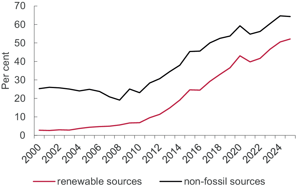
As shown in Figure 1, around one-half of natural gas in the UK is used for heating, around a third for electricity generation and the rest in industry. Crude oil is used predominantly as transport fuel and coal is almost non-existent. Figure 2 shows that, in 2023, the UK produced around 60% of its electricity needs from non-fossil sources, and over 45% from renewable sources.

Figure 1.

UK energy generation and end uses.

Source: DUKES 2026 and authors’ calculations.

Note: This figure shows how the different types of energy (left-hand side) are used in the United Kingdom (right-hand side). It shows that around one-half of natural gas in the UK is used for heating, around a third for electricity generation, and the rest in industry while crude oil is used predominantly as transport fuel and coal is negligible.

Figure 1. Long description

The diagram flows from primary energy sources on the left to end uses on the right.

Primary sources on the left include:

* Red flows: Other domestic biomass, Biomass imports, and Waste. These converge into a Bioenergy node.

* Green flows: Nuclear, Wind, Solar, and Other renewables. These, along with a portion of Bioenergy and Natural gas, flow into a yellow Electricity generation node.

* Yellow flow: Electricity imports, which flows directly into the Electricity generation node.

* Grey flows: Natural gas (the largest single source), Coal (a very thin line), and Oil.

Intermediate nodes in the center:

* Bioenergy: Splits into Transport biofuels, Industry biomass, Buildings biomass, and a flow to Electricity generation.

* Electricity generation: Splits into Buildings electricity, Industry electricity, Transport electricity, and Electricity exports.

End uses on the right:

* Natural gas flows primarily to Buildings natural gas and Industry natural gas.

* Oil flows predominantly to Transport oil, with smaller amounts to Buildings oil and Industry oil.

* Coal flows to Industry coal and Buildings coal.

* The final end-use categories are grouped into Transport, Industry, Buildings, and Exports.

Figure 2.

UK electricity generation by source.

Source: DESNZ: UK energy in brief 2026 and authors’ calculations.

Note: This figure shows the percentages of electricity generation produced from non-fossil sources (around 64% in 2025) and renewable sources (around 52% in 2025).

Figure 2. Long description

The vertical Y axis is labeled Per cent and ranges from 0 to 70 in increments of 10. The horizontal X axis represents years from 2000 to 2024 in two-year increments.

* The non-fossil sources line (black) starts at approximately 25 per cent in 2000. It remains relatively stable with a slight dip to 20 per cent in 2008 before beginning a steady upward climb. It reaches approximately 45 per cent in 2015, peaks at nearly 60 per cent in 2020, and ends at approximately 64 per cent in 2025.

* The renewable sources line (maroon) starts significantly lower at approximately 3 per cent in 2000. It shows a slow, gradual increase until 2010, after which the rate of growth accelerates. It reaches 25 per cent in 2015, approximately 43 per cent in 2020, and concludes at approximately 52 per cent in 2025.

Both lines exhibit similar fluctuations, such as a notable dip around 2021 followed by a sharp recovery, but maintain a consistent upward trajectory over the 25-year period.

Our calibration follows the approach of Batten and Millard (Reference Batten and Millard2024) and Harrison et al. (Reference Harrison, Thomas and de Weymarn2011). We first set the values for a set of standard parameters that appear in most macroeconomic models; our calibrated values are shown in Table 1. Following Harrison et al., we set the discount rate, β, to 0.9925 implying a steady-state real interest rate of 3% per annum, the intertemporal elasticity of consumption to 0.66 and the inverse Frisch elasticity of labour supply to 0.43. The cost of adjusting the foreign bond portfolio is set to 0.001. This is set to a small number so that we ensure the model has a stationary steady state, while not affecting household decisions by too much. We set the depreciation rate for capital to 10% per annum, and the elasticity of our investment adjustment cost function to 5.74.

Table 1.

Standard parameters

Table 1. Long description

The table consists of three columns: Symbol, Value, and Description.

* beta: 0.9925, Discount factor.

* sigma sub h: 0.43, Inverse Frisch elasticity of labour supply.

* sigma sub c: 0.66, Intertemporal elasticity of consumption.

* chi sub bf: 0.001, Cost of adjusting portfolio of foreign bonds.

* delta: 0.025, Depreciation rate.

* S double prime (1): 5.74, Elasticity of investment adjustment costs.

* sigma sub en: 0.4, Elasticity of substitution between non-energy and energy in consumption.

* sigma sub p: 0.1, Elasticity of substitution between petrol, gas and electricity in energy consumption.

* sigma sub q: 0.15, Elasticity of substitution between energy and everything else in non-energy production.

* sigma sub n: 0.5, Elasticity of substitution between petrol, gas and electricity in energy production.

* psi sub x: 0.24, Persistence of export demand.

* eta sub x: 1.5, Elasticity of demand for exports.

For the elasticities of substitution between non-energy and energy in consumption, σ _en, and between petrol, gas and electricity in energy consumption, σ _p, we use values of 0.4 and 0.1, again following Harrison et al. (Reference Harrison, Thomas and de Weymarn2011). We also followed that article in setting the elasticity of substitution between energy and non-energy in production, σ _q, to 0.15. But we set the elasticity of substitution between gas, petrol and electricity in energy production, σ _n, to 0.5, whereas Harrison et al. use a Leontief production function and therefore assume zero substitutability between energy types. Note that these are the values we assume in the short run. As we move towards the medium and longer runs, we allow the elasticity of substitution between the various energy sources in both consumption and production to rise, implying greater substitutability between energy inputs. In the limit, we assume a coefficient of infinity, implying perfect substitutability between energy inputs.

In terms of the parameters associated with trade, we followed Harrison et al. (Reference Harrison, Thomas and de Weymarn2011) and set the elasticity of export demand, η _x, to 1.5 and its persistence, ψ _x, to 0.24. We assume a steady state in which net exports of oil and gas are zero. Based on 2023 National Accounts data, we set steady-state government spending to 39% of aggregate consumption spending.

Second, we set a number of parameters to ensure that steady-state shares in the model matched their average values in the UK data. These are shown in Table 2. We use the 2021 CPI weights to set ψ _e equal to 4.8%, ψ _g to 0.25 and ψ _p to 0.3541. The 2018 SUTs allow us to set α _q to 0.0438 to match the share of energy in the non-energy producing firms’ total costs, α _B to 0.2326 to match the share of imported intermediates in non-energy-producing firms’ non-energy costs and $ {\alpha}_{k,q}\hskip0.32em $ to 0.3424 to match the share of labour in non-energy-producing firms’ non-energy costs. Similarly, we set ψ _n,p, ψ _n,g and ψ _n,e to 0.3135, 0.1478 and 0.5387, respectively, so as to match the cost shares of petrol, gas and electricity in production of the non-energy goods. Finally, data from the 2018 SUTs suggest that the labour share in electricity costs is 0.0689 and the share of gas in electricity costs is 0.1416.

Table 2.

Parameters set to match spending, cost and revenue shares

Table 2. Long description

The table consists of three columns: Parameter, Value, and Description.

* alpha sub q: 0.0438. Set to match the cost share of energy in non-energy production.

* alpha sub k q: 0.3424. Set to match the cost share of labour in non-energy production.

* alpha sub b: 0.2326. Set to match the cost share of imports in non-energy production.

* alpha sub k u: 0.7895. Set to match the cost share of gas in electricity production.

* alpha sub h u: 0.0689. Set to match the cost share of labour in electricity production.

* psi sub e: 0.0480. Share of energy in household consumption spending.

* psi sub g: 0.2500. Share of gas in household spending on energy.

* psi sub p: 0.3541. Share of petrol in household spending on energy.

* psi sub n,p: 0.3135. Set to match the cost share of petrol in non-energy production.

* psi sub n,g: 0.1478. Set to match the cost share of gas in non-energy production.

Finally, we follow Batten and Millard (Reference Batten and Millard2024) in setting the parameters governing the carbon emissions associated with household consumption of petrol and gas and petrol and gas used in the production of electricity and non-energy goods. This is so that we can apply a tax of a given amount per kilogram of CO₂ emissions. Specifically, we use the UK Government GHG conversion factors for company reporting and we apply the 2021 values in our work. We set $ {\varpi}_{p,c} $ , $ {\varpi}_{p,q} $ , $ {\varpi}_{g,c} $ , $ {\varpi}_{g,q} $ and $ {\varpi}_{g,e} $ to 1.586, 2.081, 4.568, 4.568 and 4.568, respectively. Given our calibration, this implies that a carbon tax of £100 per tonne of CO₂ emissions would correspond to a τ _c of 0.081.

5. The short- and medium-run effects of a permanent increase in the carbon tax

In this section, we model the effect of a permanent increase in the carbon tax, τ_c, from zero to £100 per tonne of CO₂ emissions in both the short and medium runs. We start by considering the short-run effects of this change, where we assume that petrol and gas are complements to green inputs in production and are complements to electricity and non-energy goods and services in consumption.

5.1. Short-run effects

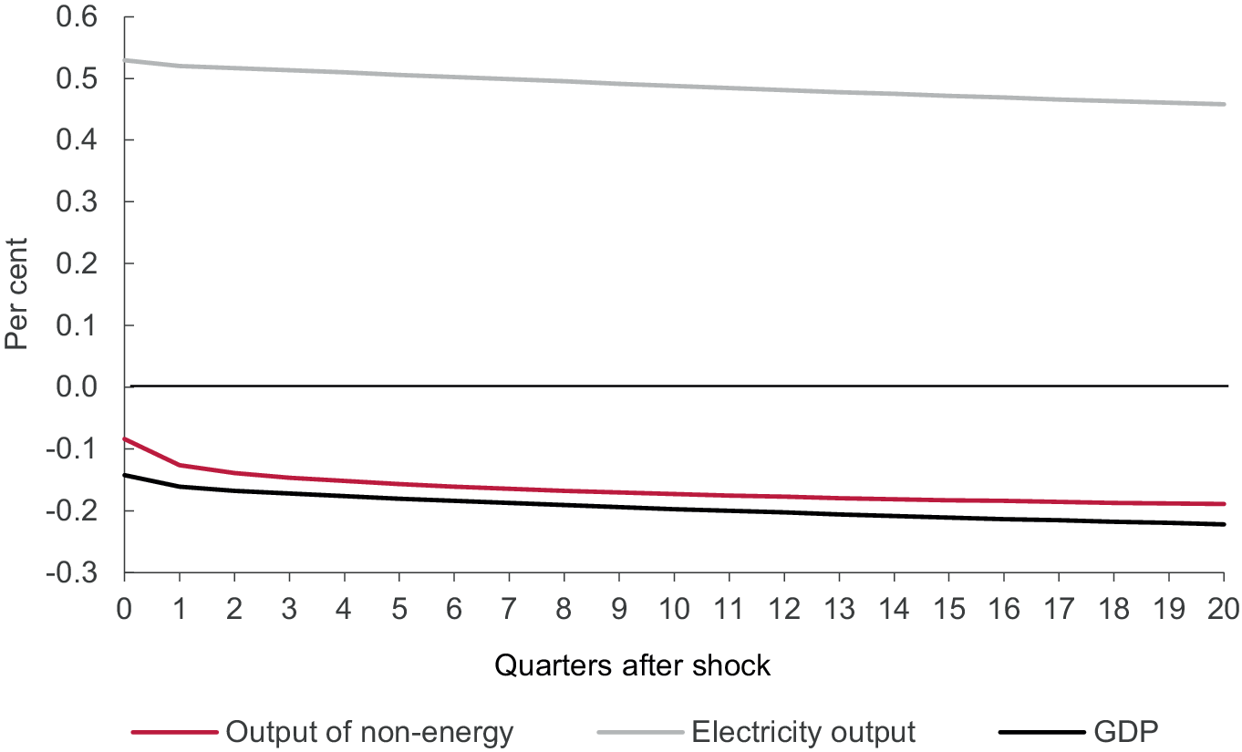
Figure 3 shows that the introduction of the carbon tax results in an increase in production of electricity, as firms and households immediately switch away from carbon-emitting fuels towards electricity, given that it is now relatively cheaper. However, since petrol and gas are complements in production with green inputs, the increase in their cost leads to an immediate reduction in gross output of non-energy goods. And since non-energy production forms the bulk of output in the economy, GDP also falls. If we assumed that electricity production relies to some degree on imported intermediates, then the effect on GDP would likely be larger, as the shift to electricity in production would lead to an increase in imports above and beyond the increase that already resulted from the shift towards imported intermediates in production of non-energy goods.

Figure 3.

Response of gross output and GDP to the imposition of a carbon tax.

Note: This figure shows that applying a permanent carbon tax of £100 per tonne of CO₂ emissions reduces GDP and output in the non-energy sector while raising output in the electricity sector.

Figure 3. Long description

The X-axis is labeled Quarters after shock and ranges from 0 to 20 in increments of 1. The Y-axis is labeled Per cent and ranges from negative 0.3 to 0.6 in increments of 0.1. A horizontal baseline is set at 0.0.

Three distinct lines represent the data trends:

* Electricity output: A light gray line starting at approximately 0.53 at quarter 0. It shows a slight, steady downward slope, ending at approximately 0.46 by quarter 20.

* Output of non-energy: A dark red line starting at approximately negative 0.08 at quarter 0. It drops sharply to negative 0.13 by quarter 1 and then continues a gradual decline to approximately negative 0.19 by quarter 20.

* G D P: A thick black line starting at approximately negative 0.14 at quarter 0. It follows a similar trajectory to the non-energy output, declining steadily to reach its lowest point at approximately negative 0.22 by quarter 20.

After the initial falls, gross output of non-energy goods and GDP continue to fall over time given the permanent increase in costs for non-energy producers and the fall in household demand. And this fall in gross output of non-energy goods leads to a fall in electricity production given the lower need for electricity input, and the fact that electricity input is complementary to inputs of gas and petrol.

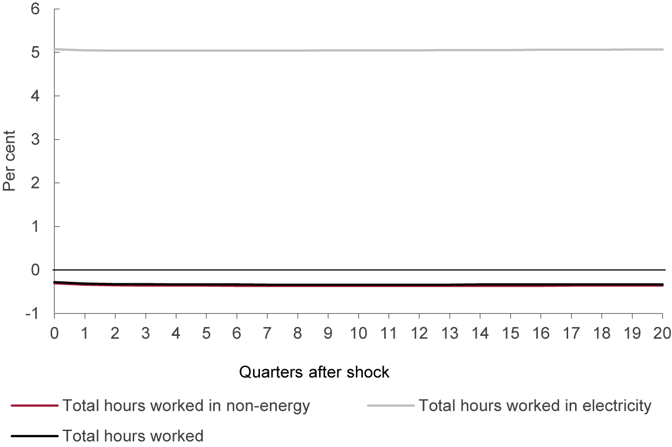
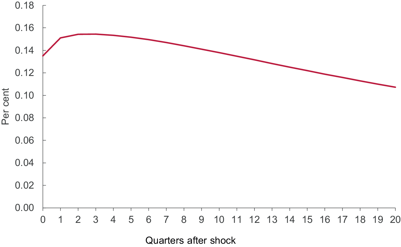
Figure 4 shows that the increased production of electricity leads to an immediate and permanent rise in total hours worked in the electricity sector. At the same time, the fall in output in the non-energy sector is associated with an immediate and permanent fall in total hours worked in the non-energy sector. Given that the bulk of total hours (99.5% in steady state) are worked in the non-energy sector, the net result is an immediate and permanent fall in aggregate total hours. Since the initial fall in GDP is smaller than the fall in total hours, labour productivity rises following the introduction of the carbon tax, as shown in Figure 5, though this effect is small. But as GDP continues to fall while total hours are stable, labour productivity then starts to fall back. Five years after the tax is imposed, labour productivity is around 0.1% higher than before the tax was imposed.

Figure 4.

Response of hours to imposition of a carbon tax.

Note: This figure shows that applying a permanent carbon tax of £100 per tonne of CO₂ emissions reduces hours worked in the non-energy sector while raising hours worked in the electricity sector.

Figure 4. Long description

The line graph plots Per cent on the Y-axis, ranging from minus 1 to 6, against Quarters after shock on the X-axis, ranging from 0 to 20. A horizontal baseline is set at 0.

Three distinct lines represent the data trends.

1. Total hours worked in electricity is represented by a light gray line at the top of the plot. It maintains a nearly flat, horizontal trajectory at approximately 5 per cent throughout the entire 20-quarter period.

2. Total hours worked is represented by a solid black line. It starts slightly below 0 at quarter 0 and remains relatively stable, trending very slightly downward to settle just above the minus 0.5 mark.

3. Total hours worked in non-energy is represented by a dark red line. This line is positioned almost identically to the black line, starting just below 0 and following a parallel path that settles around minus 0.5 per cent, indicating a slight decrease in hours worked over the 20 quarters.

Figure 5.

Response of labour productivity to imposition of a carbon tax.

Note: This figure shows that applying a permanent carbon tax of £100 per tonne of CO₂ raises labour productivity.

Figure 5. Long description

The Y axis is labeled Per cent and ranges from 0.00 to 0.18 in increments of 0.02. The X axis is labeled Quarters after shock and ranges from 0 to 20 in increments of 1. A single dark red line begins at approximately 0.135 at quarter 0. It rises sharply to a peak of roughly 0.155 at quarter 2. Following this peak, the line exhibits a gradual, near-linear decline, ending at approximately 0.11 by quarter 20.

5.2. Medium-run effects

In the medium run, both households and non-energy producers become more able to substitute away from petrol and gas towards electricity. To examine how this might affect the response of productivity to the carbon tax, we again examined the effect of a permanent increase in the carbon tax, τ_c, from zero to £100 per tonne of CO₂ emissions but under different assumptions about the degree of substitutability of petrol and gas for electricity in consumption and non-energy production: specifically, we compared our benchmark case where electricity complements petrol and gas ( $ {\sigma}_p=0.1 $ and $ {\sigma}_n=0.5 $ ) against the Cobb–Douglas case and against a case where electricity is a substitute for petrol and gas ( $ {\sigma}_p={\sigma}_n=2 $ ). For the purposes of the experiment, we maintained our assumption of Cobb–Douglas technology in the production of electricity.

Although our approach to modelling the difference between the short and medium runs—that is, that we can think of two separate models with different parameter values—is common for tractability in DSGE models, it is somewhat ad hoc. Footnote ³ Ideally, we would wish to model the transition from the short to medium run via a gradual, endogenous change in these elasticities, which would better reflect the actual path of technological change. Indeed, Jo and Miftakhova (Reference Jo and Miftakhova2022) do this, finding that, as firms are incentivised to switch out of fossil fuels into clean energy sources, they make technological improvements that themselves make clean energy more substitutable for fossil fuels over time. However, we feel that for the purposes of our article, modelling a gradual evolution of the elasticities would overly complicate the model without altering our key insights on how productivity is likely to respond to the green transition.

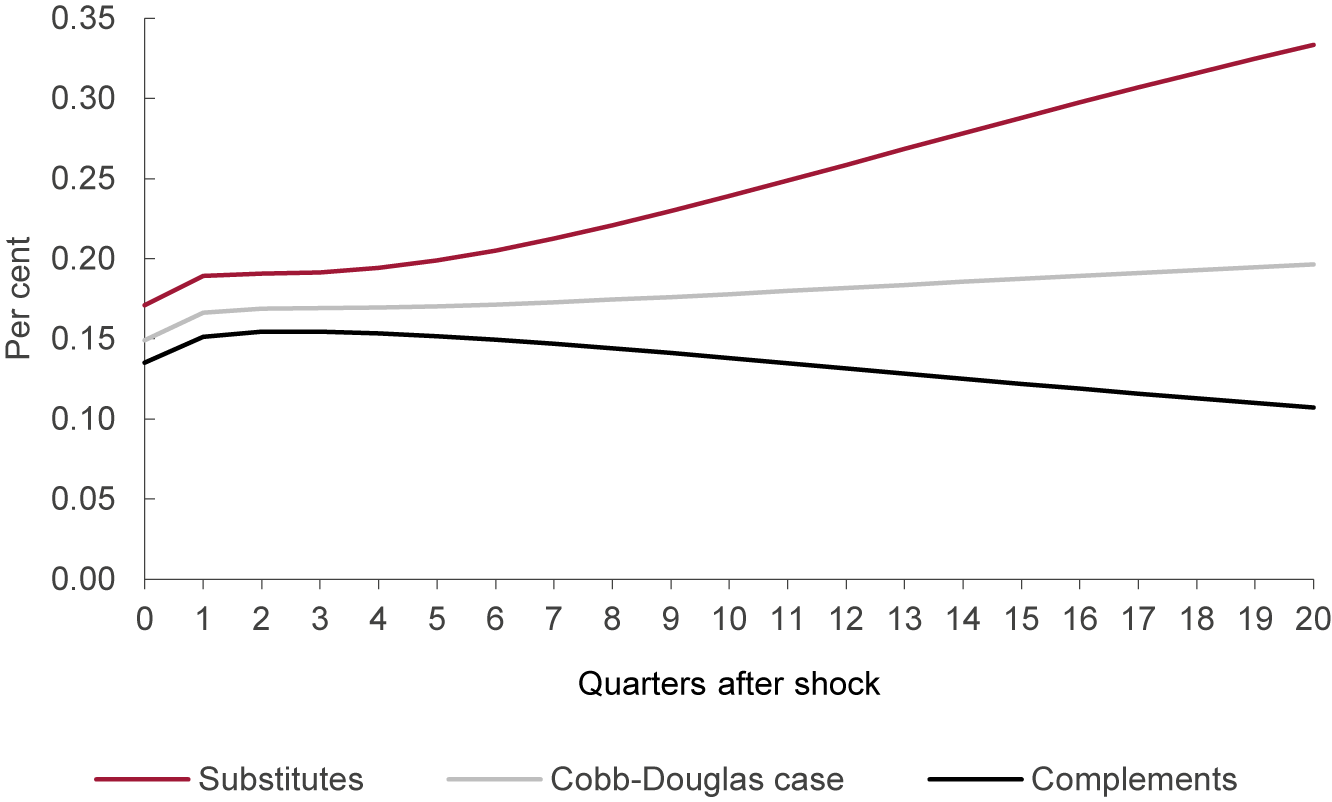
Figure 6 shows the response of productivity to the imposition of a carbon tax in the three cases. As can be seen, in the case where electricity, gas and petrol are complements, the rise in productivity is short-lived, given output continues to fall over time while total hours—after the initial fall—stabilise, as shown in Figure 4. However, in the Cobb–Douglas case, and the case where electricity is a substitute for petrol and gas, productivity rises initially (as GDP falls by less than total hours) but then continues to rise as GDP recovers while total hours remain permanently lower than initially. The higher the degree of substitution between electricity, petrol and gas, the more productivity increases in response to the carbon tax. Again, however, the more that electricity production using renewables depends on imported intermediates, the smaller will be the rise in productivity.

Figure 6.

Response of labour productivity to imposition of a carbon tax.

Note: This figure shows that the effect of a carbon tax on productivity depends on the elasticity of substitution between electricity and fossil fuels, with the effect being larger when the energy inputs are more substitutable, as we would expect to be the case over time.

Figure 6. Long description

The vertical Y axis is labeled Per cent and ranges from 0.00 to 0.35 in increments of 0.05. The horizontal X axis is labeled Quarters after shock and ranges from 0 to 20 in increments of 1. Three lines originate between 0.13 and 0.17 on the Y axis at quarter 0.

* The top line, colored dark red, represents Substitutes. It shows a sharp initial increase to 0.19 at quarter 1, plateaus briefly, and then follows a steady upward curve reaching approximately 0.33 by quarter 20.

* The middle line, colored light gray, represents the Cobb-Douglas case. It rises to 0.17 at quarter 1 and maintains a very gradual, near-linear upward slope, ending just below 0.20 at quarter 20.

* The bottom line, colored black, represents Complements. It rises to 0.15 at quarter 1, peaks at quarter 2, and then enters a long-term gradual decline, ending at approximately 0.11 by quarter 20.

5.3. Robustness checks

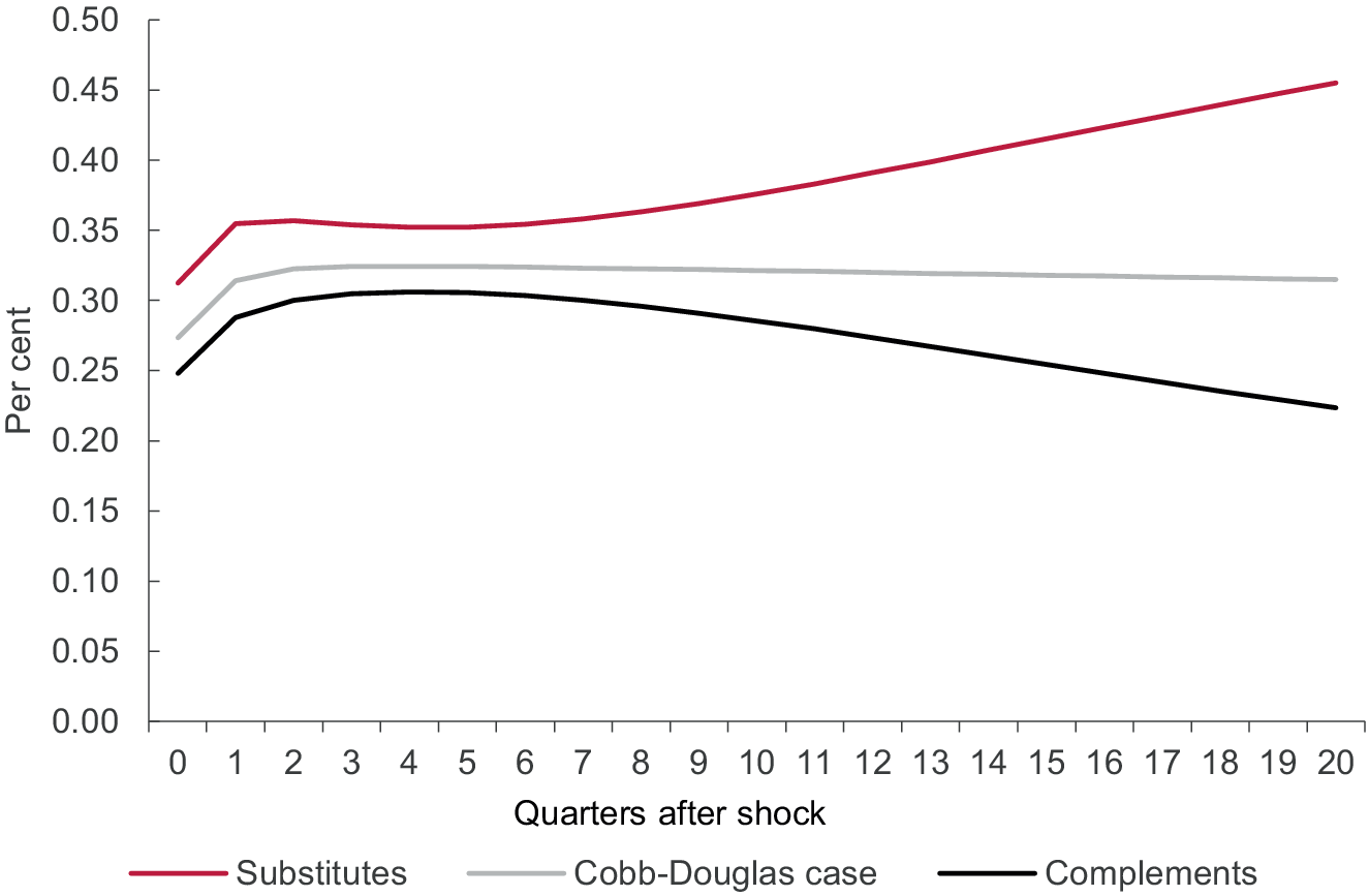
We carried out a number of robustness checks on the results as summarised in Figure 6. We first looked at the effect of making labour supply more inelastic. More specifically, we set the Frisch elasticity of labour supply equal to 0.5 (as opposed to 2.33 in our baseline case). The response of productivity to the imposition of a carbon tax is shown in Figure 7. Although productivity initially rises by more the more inelastic is labour supply, the patterns of the responses are the same with productivity continuing to rise when electricity is a substitute for petrol and gas while it eventually falls back when electricity, petrol and gas are complements.

Figure 7.

Response of labour productivity to imposition of a carbon tax with inelastic labour supply.

Note: This figure shows that the effect of a carbon tax on productivity is initially greater when labour supply is more inelastic.

Figure 7. Long description

The x-axis is labeled Quarters after shock and ranges from 0 to 20 in increments of 1. The y-axis is labeled Per cent and ranges from 0.00 to 0.50 in increments of 0.05. Three lines represent different scenarios.

* Substitutes (red line): Starts at approximately 0.31, rises sharply to 0.35 by quarter 1, remains relatively flat until quarter 6, and then exhibits a steady upward linear increase, ending at approximately 0.46 at quarter 20.

* Cobb-Douglas case (grey line): Starts at approximately 0.27, rises to 0.32 by quarter 2, and remains almost perfectly horizontal at that level through quarter 20.

* Complements (black line): Starts at approximately 0.25, peaks at 0.31 around quarter 4, and then follows a gradual downward curve, ending at approximately 0.22 at quarter 20.

A legend at the bottom identifies the red line as Substitutes, the grey line as Cobb-Douglas case, and the black line as Complements.

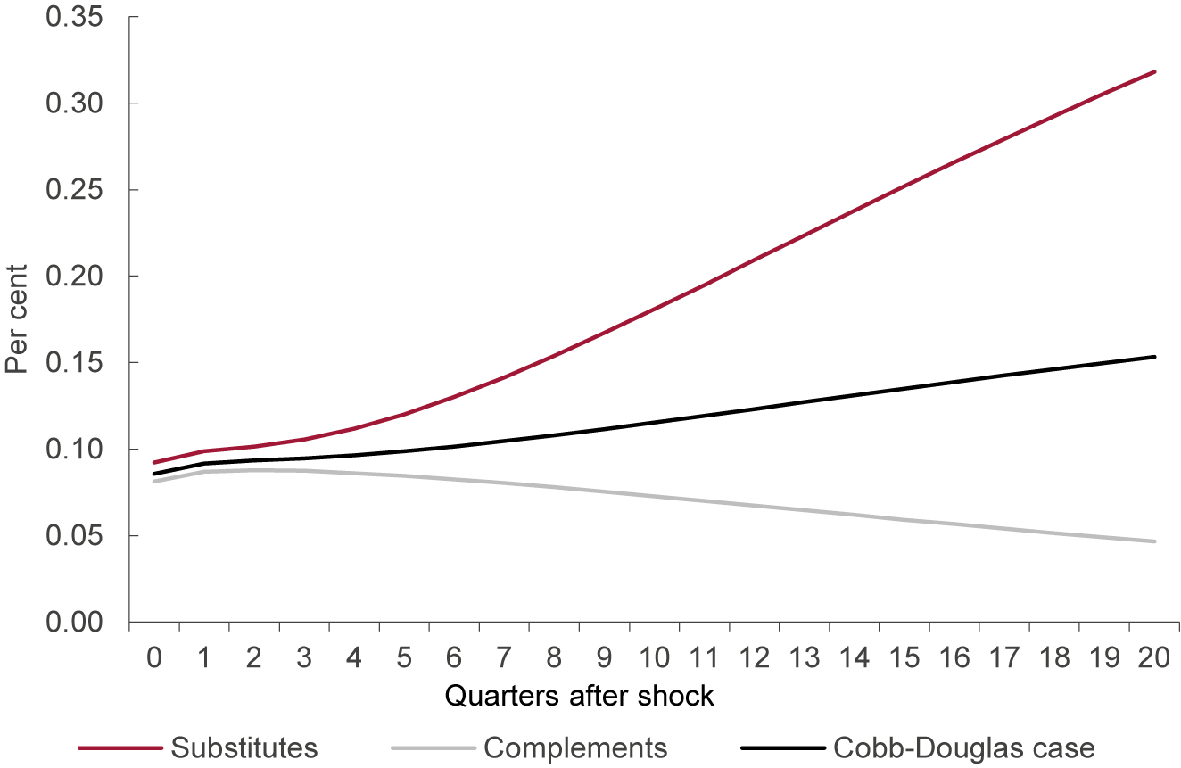
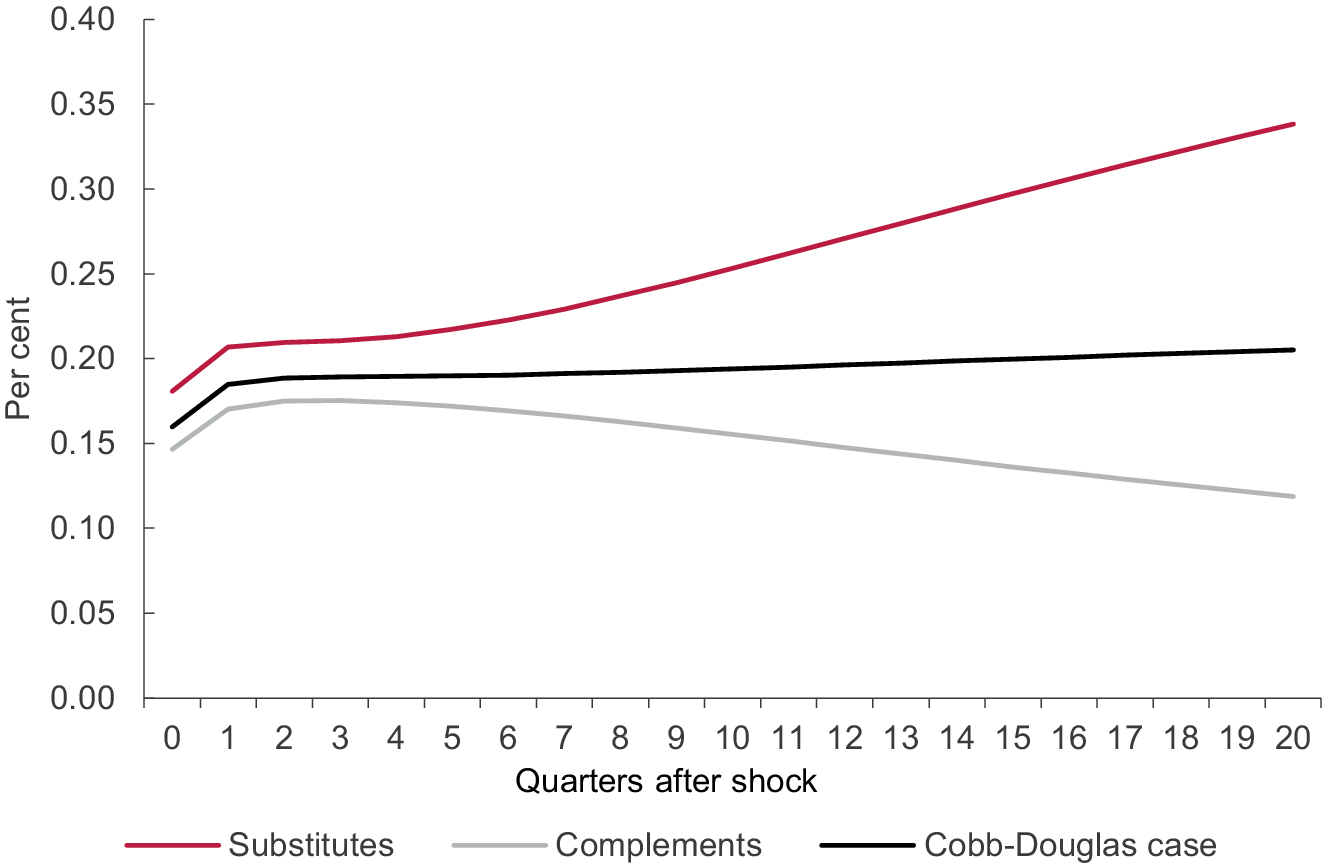
We then looked at the effect of making households more risk averse. Specifically, we set the coefficient of relative risk aversion in the utility function equal to 5 (as opposed to 0.66 in our baseline case). The results are shown in Figure 8. In this case, productivity initially rises by less when households are more risk averse, but again, the patterns of the responses are the same, with productivity continuing to rise when electricity is a substitute for petrol and gas, while it eventually falls back when electricity, petrol and gas are complements. In the Cobb–Douglas case, productivity continues to rise after the initial increase, as in the baseline case, though it rises at a faster rate. Staying with households, we also looked at the effect of making energy and non-energy goods substitutes in consumption, raising the elasticity of substitution between them from 0.4 to 2. The results are shown in Figure 9 and are very similar to the baseline results.

Figure 8.

Response of labour productivity to imposition of a carbon tax with more risk-averse households.

Note: This figure shows that the effect of a carbon tax on productivity is initially greater when households are less risk averse.

Figure 8. Long description

The horizontal X axis is labeled Quarters after shock and ranges from 0 to 20 in increments of 1. The vertical Y axis is labeled Per cent and ranges from 0.00 to 0.35 in increments of 0.05. Three lines originate near the 0.08 to 0.10 range at quarter 0 and diverge as time progresses.

* The Substitutes line, colored dark red, shows a steep upward trend, rising from approximately 0.09 at quarter 0 to over 0.30 by quarter 20.

* The Cobb-Douglas case line, colored black, shows a moderate linear increase, rising from approximately 0.085 at quarter 0 to about 0.15 at quarter 20.

* The Complements line, colored light grey, initially rises slightly until quarter 1 and then follows a steady downward asymptotic curve, ending near 0.05 at quarter 20.

A legend at the bottom identifies the three series from left to right as Substitutes, Complements, and Cobb-Douglas case.

Figure 9.

Response of labour productivity to imposition of a carbon tax with energy and non-energy substitutes in consumption.

Note: This figure shows that the effect of a carbon tax on productivity depends on the elasticity of substitution between electricity and fossil fuels, with the effect being larger when energy inputs are more substitutable, and that, quantitatively, this does not depend on the substitutability of energy and non-energy in consumption.

Figure 9. Long description

The X-axis is labeled Quarters after shock and ranges from 0 to 20 in increments of 1. The Y-axis is labeled Per cent and ranges from 0.00 to 0.40 in increments of 0.05. Three lines originate near 0.15 to 0.18 at quarter 0.

* The top line, colored red and labeled Substitutes, shows a sharp initial increase to 0.21 by quarter 1, followed by a steady upward linear trend reaching approximately 0.34 by quarter 20.

* The middle line, colored black and labeled Cobb-Douglas case, shows a smaller initial increase to 0.18 by quarter 1, followed by a very gradual upward slope, ending at approximately 0.21 by quarter 20.

* The bottom line, colored grey and labeled Complements, shows an initial rise to 0.17 by quarter 2, followed by a gradual downward trend, ending at approximately 0.12 by quarter 20.

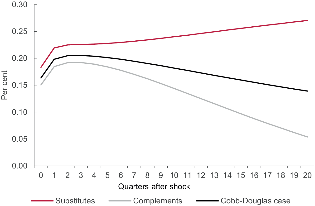
Our final robustness check was to look at how the response of productivity to the imposition of a carbon tax is affected by the substitutability of energy and non-energy in production. Specifically, we raised the elasticity of substitution between energy and non-energy in production from 0.15 to 2. The results are shown in Figure 10. In this case, we find that the initial positive effect on productivity is quickly reversed in both the baseline case—where electricity, gas and petrol are complements—and the Cobb–Douglas case with unitary elasticity of substitution between the three energy sources. Productivity continues to rise beyond the initial increase where electricity, gas and petrol are complements, but at a slower rate than in the baseline.

Figure 10.

Response of labour productivity to imposition of a carbon tax with energy and non-energy substitutes in production.

Note: This figure shows that, when energy and non-energy inputs are more substitutable in production, the initial positive effect of a carbon tax on productivity is quickly reversed in the baseline and Cobb–Douglas cases.

Figure 10. Long description

The x-axis is labeled Quarters after shock and ranges from 0 to 20 in increments of 1. The y-axis is labeled Per cent and ranges from 0.00 to 0.30 in increments of 0.05. Three lines represent different production scenarios.

* Substitutes (red line): Starts at approximately 0.18 at quarter 0, rises sharply to 0.22 by quarter 1, and then continues a steady, slightly concave upward climb to reach approximately 0.27 by quarter 20.

* Cobb-Douglas case (black line): Starts at approximately 0.16 at quarter 0, peaks at roughly 0.21 around quarter 3, and then enters a gradual linear decline, ending at approximately 0.14 by quarter 20.

* Complements (light gray line): Starts at approximately 0.15 at quarter 0, peaks at roughly 0.19 around quarter 3, and then declines more steeply than the other two lines, ending at approximately 0.05 by quarter 20.

A legend at the bottom identifies the lines from left to right as Substitutes, Complements, and Cobb-Douglas case.

6. The long-run effects of a move to net zero

In the long run, we would expect to see electricity replace gas and petrol completely in consumption and in the production of non-energy goods, and we would expect to see renewables completely replace gas in the production of electricity. In addition, we would expect production of oil and gas to be phased out. In this section, we examine the effects on productivity of such a redirection of economic activity in the United Kingdom.

6.1. A ‘net zero’ steady state

We first consider what a ‘net zero’ steady state might look like. As is well known, to move to a net zero steady state requires a significant amount of investment in ‘green capital’; in our model, this is the capital used in the production of electricity. One might expect such investment to raise productivity via a ‘capital deepening’ effect. To show that that is the case, and to begin to suggest how much investment might be needed, we consider an experiment in which consumption remains unchanged across the two steady states, that is the current situation and the ‘net zero’ economy.

Table 3 gives the values of a number of variables of interest relative to steady-state consumption. The assumption underlying this table is that households switch their entire consumption of energy into electricity; there is therefore no reduction in aggregate consumption nor consumption of energy. In practice, this means that households replace their internal combustion engine cars with electric vehicles and their gas boilers with electric heat pumps. As a result, consumption of electricity is increased by over 150%. These model predictions are consistent with the prediction of the Climate Change Committee’s Balanced Net Zero Pathway (CCC, 2020), which forecast a doubling in demand for electricity as a result of increasing electrification of the economy (e.g. use of electric vehicles in transport), from around 300 TWh in 2020 to 677 TWh in 2050.

Table 3.

Steady-state effects of moving to net zero

Table 3. Long description

The table contains four columns: Indicator, Initial steady state, Net zero steady state, and Percentage difference.

* Aggregate consumption: 1.0000 to 1.0000 (0.00 percent difference).

* Consumption of non-energy goods: 0.9520 to 0.9520 (0.00 percent difference).

* Consumption of electricity: 0.0190 to 0.0480 (152.63 percent increase).

* Output of non-energy goods: 2.6443 to 2.7810 (5.17 percent increase).

* Output of electricity: 0.0814 to 0.1698 (108.60 percent increase).

* Total hours worked in the non-energy sector: 0.9948 to 1.0224 (2.77 percent increase).

* Total hours worked in the electricity sector: 0.0052 to 0.0106 (103.85 percent increase).

* Capital in the non-energy sector: 26.5924 to 27.9670 (5.17 percent increase).

* Capital in the electricity sector: 1.9739 to 4.8564 (146.03 percent increase).

* Imports of non-energy intermediates: 0.5881 to 0.6185 (5.17 percent increase).

* G D P: 2.1042 to 2.2105 (5.05 percent increase).

* Labour productivity: 2.1042 to 2.1399 (1.70 percent increase).

Given higher demand for electricity from both households and non-energy producers, the producers of electricity need to expand their output dramatically, by more than double. But they will be doing this at the same time as switching from using gas to generate electricity towards using renewables. This leads them to increase their capital stock (‘green capital’) by almost 150%. This would require a huge increase in investment, again consistent with the Climate Change Committee’s (CCC, 2025) view that an additional £238 billion of capital expenditure will be needed in the electricity industry over the 15 years between 2025 and 2040 for the UK economy to achieve its net zero target.

To supply the additional physical capital, and to increase exports to pay for the increase in imported intermediates, non-energy producers need to raise their output, by a little over 5%. They produce this additional output by using more electricity, labour and capital. Again, the need for a higher capital stock beyond the electricity sector was noted by the Climate Change Committee (CCC, 2025), which suggests that an additional £244 billion of investment in housing and £104 billion of investment elsewhere is needed between 2025 and 2040 for the UK economy to achieve its net zero target. We can also note that firms increase their imports of intermediates in the model. We can note that, if we assumed that renewable energy production required imported intermediates, then the rise in imports would be even larger.

The result of this increase in activity is that GDP increases by just over 5%. But, because total hours have also increased, productivity only rises by 1.7%. To be clear, these results do not imply that the move to net zero leads to higher productivity. Rather they just confirm that, if the economy is to move to net zero without a detrimental effect on long-run consumption, then its capital stock has to increase substantially and labour productivity with it. Unless we can increase productivity, the green transition will lead to a reduction in consumption.

6.2. Spillovers from green technologies

One interesting question from a policy perspective is whether the green transition on its own can lead to technological improvements that would raise productivity above and beyond the pure effect of ‘capital deepening’ considered here. That is, could the move from carbon-emitting technology to green technology lead to higher GDP growth in the economy via spillovers from green investment—specifically in the electricity sector—to the rest of the economy? In the rest of this section of the article, we modify our model to allow for this possibility.

In the absence of gas as an input, the production function for electricity will be given by:

(27) $$ {q}_{e,t}={A}_e\hskip0.32em {k}_{e,t}^{1-{\alpha}_{h,u}}{h}_{e,t}^{\alpha_{h,u}}. $$

We assume that non-energy producers can no longer use petrol and gas in production. We also assume that investment in renewable energy production in the electricity sector gives rise to production externalities in the non-energy sector. Putting these assumptions together, we now assume that the production function for non-energy will be given by:

(28) $$ {q}_t={\left({\left(1-{\alpha}_q\right)}^{\frac{1}{\sigma_q}}{\left(A{k}_{e,t}^{\xi }{\left({k}_{NE,t}\right)}^{\alpha_{k,q}}{h}_{NE,t}^{1-{\alpha}_{k,q}-{\alpha}_B}{M}_t^{\alpha_B}\right)}^{\frac{\sigma_q-1}{\sigma_q}}+{\alpha}_q^{\frac{1}{\sigma_q}}{I}_{e,t}^{\frac{\sigma_q-1}{\sigma_q}}\right)}^{\frac{\sigma_q}{\sigma_q-1}}. $$

Where the presence of k _e—the capital stock used in electricity production—in the production function for non-energy is what gives rise to the spillovers. This modelling approach has been used previously in, for example, Ramey (Reference Ramey2020) and other work in the endogenous growth literature where technological advance in one sector leads to higher productivity in other sectors (Aghion and Howitt, Reference Aghion and Howitt2009). Stern and Stiglitz (Reference Stern and Stiglitz2023) suggest reasons why we might expect an increase in green investment—capital stock in the electricity sector in the model—to result in higher productivity in the rest of the economy. In a recent study for France, Pisani-Ferry and Mahfouz (Reference Pisani-Ferry and Mahfouz2023) note that recent progress in many key areas, such as battery technologies, electric vehicles and heat pumps have already shown that shifting to green technologies can lead to higher productivity and lower costs.

In what follows, we examine the effects of an increase in investment in the electricity sector on growth in the economy under different assumptions about the value of ξ. We implement an exogenous increase in investment via an investment-specific technology shock. More precisely, we rewrite equation (6) as:

(29) $$ {k}_t=\left(1-\delta \right){k}_{t-1}+{\varepsilon}_{i,t}\left(1-S\left(\frac{I_t}{I_{t-1}}\right)\right){I}_t. $$

where ε _i denotes the investment-specific technology shock. Following the results reported in Smets and Wouters (Reference Smets and Wouters2007), we assume that the shock follows an AR(1) process with an autocorrelation coefficient of 0.7. We consider the effects of a 1% shock to investment in the case of ξ equal to zero, 0.05 and 0.2. In each case, we decompose the effect on labour productivity into that which can be attributed to capital deepening and that which can be attributed to the spillovers from the increased investment in the electricity sector to the non-energy sector, $ \frac{\partial lny}{\partial {lnI}_e}\approx \xi ln{k}_e $ .

Figures 11 through 13 show our results.

Figure 11.

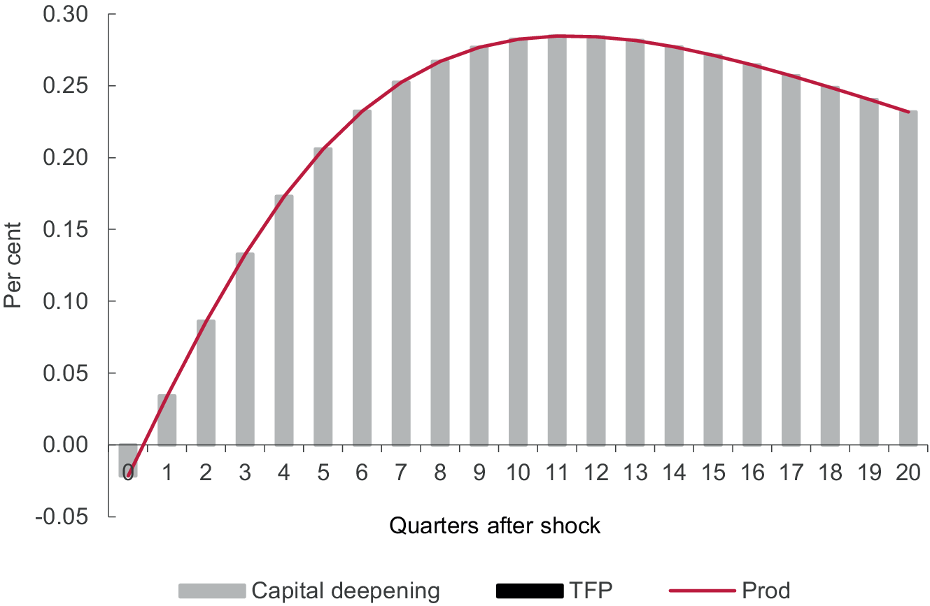
Effect of an investment-specific technology shock with no spillovers.

Note: This figure shows the effect of an increase in investment in the electricity on productivity when there are no spillovers to productivity in the non-energy sector.

Figure 11. Long description

The X axis is labeled Quarters after shock and ranges from 0 to 20. The Y axis is labeled Per cent and ranges from negative 0.05 to 0.30. A legend at the bottom identifies three variables. Capital deepening is represented by light gray vertical bars. T F P is represented by a black bar, though it is not visible in the main plot area. Prod is represented by a solid red line.

At quarter 0, the Capital deepening bar and the Prod line both start slightly below the zero line at approximately negative 0.02. From quarter 1 to quarter 11, both the bars and the line show a steep concave increase. The Prod line and Capital deepening bars track each other almost perfectly. The peak occurs between quarters 11 and 12 at approximately 0.28 per cent. From quarter 13 to 20, there is a gradual linear decrease, ending at approximately 0.23 per cent at quarter 20.

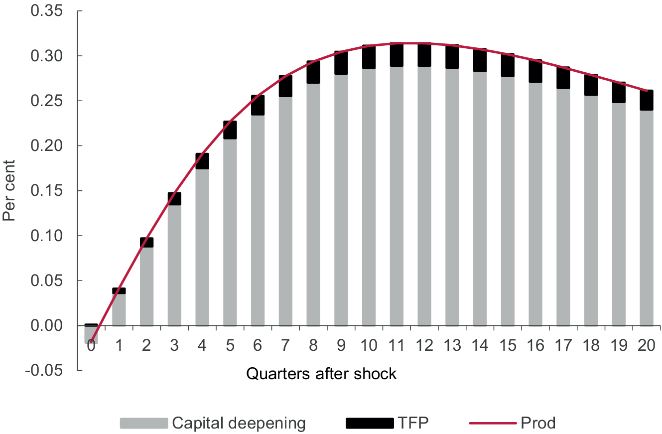
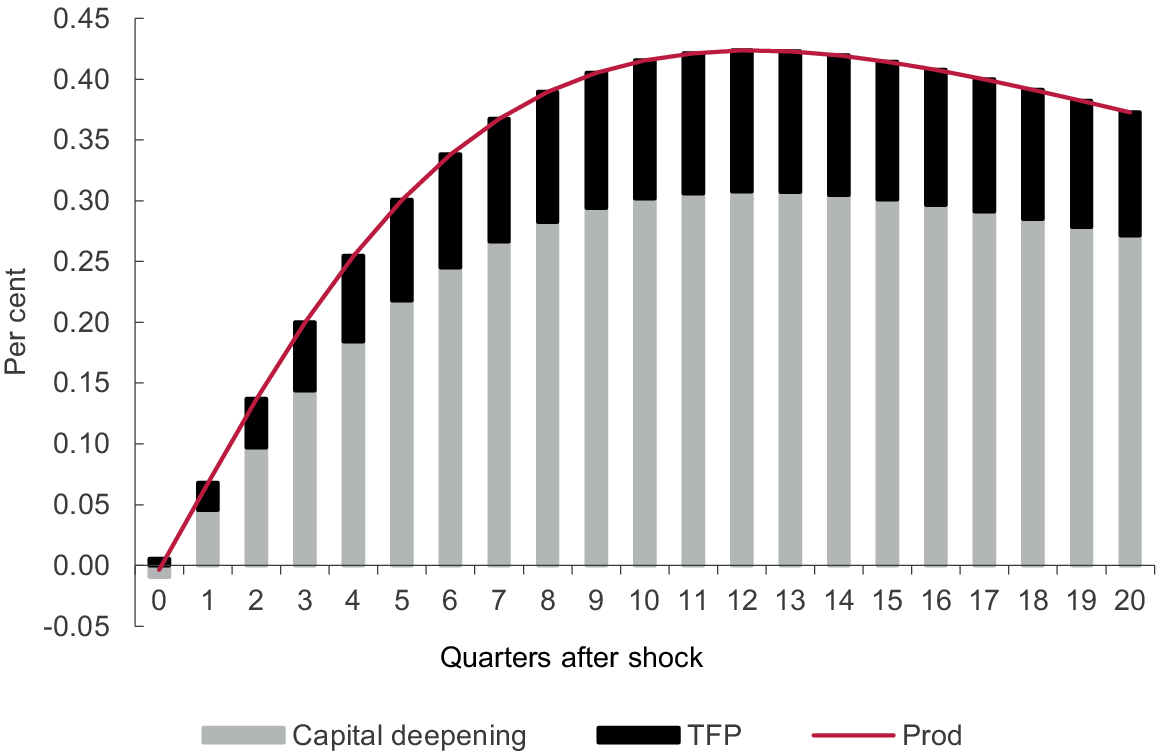
Figure 11 shows that a 1% increase in the efficiency with which investment is turned into capital leads to an increase in productivity in the net zero economy with no spillovers of just under 0.3% after two and a half years. This increase in productivity is the result of the capital deepening that occurs in response to an investment-specific technology shock. When we allow for the presence of spillovers, this effect remains but is enhanced by the spillover effect coming from increased capital in the electricity sector (‘green capital’) affecting the productivity of other sectors. Figure 12 suggests that with an elasticity of gross non-energy output to capital in the electricity sector of 0.05, the spillover effects are small, roughly 0.025% after two and a half years. Increasing this elasticity to a value of 0.2—which is large relative to the numbers used in similar models—only increases this impact to 0.12%, that is, only around one-third of the effect of capital deepening (Figure 13). Of course, these results are only illustrative as we are not sure what spillover effects might result from the green transition. But they do suggest that, unless investment in green technology leads to significant technological gains elsewhere, it is unlikely that the move to net zero will have a large effect on productivity growth above and beyond the direct effect resulting from the capital deepening that will be associated with it.

Figure 12.

Effect of an investment-specific technology shock with ξ = 0.05.

Note: This figure shows the effect of an increase in investment in the electricity on productivity when spillovers are small.

Figure 12. Long description

The vertical Y axis is labeled Per cent and ranges from negative 0.05 to 0.35 in increments of 0.05. The horizontal X axis is labeled Quarters after shock and ranges from 0 to 20.

Data is presented as stacked bars with a red line overlay.

* The grey portion of the bars represents Capital deepening.

* The black portion of the bars represents T F P.

* The red line represents Prod.

At quarter 0, the bar is slightly negative, around negative 0.02. From quarter 1 to quarter 11, there is a steady concave increase. Capital deepening makes up the majority of the value, while T F P contributes a small, increasing segment at the top of each bar. The total value peaks at quarter 11 at approximately 0.32 per cent. From quarter 12 to 20, the values show a gradual linear decrease, ending at approximately 0.26 per cent. The red line for Prod closely follows the top edge of the stacked bars throughout the entire 20 quarter period.

Figure 13.

Effect of an investment-specific technology shock with ξ = 0.2.

Note: This figure shows the effect of an increase in investment in the electricity on productivity when spillovers are large. Even with large spillovers, 75% of the effect of the increased investment on productivity results from capital deepening.

Figure 13. Long description

The X axis is labeled Quarters after shock and ranges from 0 to 20. The Y axis is labeled Per cent and ranges from negative 0.05 to 0.45.

Three data series are presented.

1. Capital deepening is represented by light gray bars.

2. T F P is represented by black bars stacked on top of the gray bars.

3. Prod is represented by a solid red line that follows the total height of the stacked bars.

At quarter 0, the values are near zero. From quarters 1 to 12, there is a steady concave increase. Capital deepening (gray) rises from approximately 0.05 at quarter 1 to a peak of 0.30 at quarter 12. T F P (black) begins to contribute significantly at quarter 2 and grows to a thickness of about 0.12 by quarter 12.

The total productivity (red line) peaks at quarter 12 at approximately 0.42 per cent. From quarters 13 to 20, there is a gradual decline, with the red line ending at approximately 0.37 per cent. Throughout the entire period, the light gray Capital deepening section remains the dominant component, accounting for roughly three-quarters of the total height.

7. Conclusions and next steps

In this article, we have constructed a DSGE model of a small open economy with four sectors: households, firms, the government and the rest of the world. We developed our model to analyse the impact of the transition to net zero on the macroeconomy. For this purpose, we included two types of energy sources: fossil fuels (specifically, oil, gas and gas-generated electricity) and electricity generated using renewables. We showed that the introduction of a carbon tax to encourage the move towards net zero has the effect of shifting the production of electricity from fossil fuels to renewable sources, as well as shifting consumption away from petrol and gas towards electricity. The overall effect was to reduce GDP and total hours worked, but since total hours fell by more than GDP, productivity increased as a result of the carbon tax.

We argued that, in the medium run, electricity would become more substitutable for petrol and gas. Our model implies that, as this happens, the effect on productivity becomes more positive as GDP recovers while total hours worked remain permanently lower than initially. We found that to maintain consumption through the transition to net zero, total hours would need to increase, as would productivity. More importantly, to get to net zero at the same level of consumption would require an increase in the aggregate capital stock of around 15% but an increase of just under 150% in the capital stock within the electricity sector, which we can think of as ‘green’ capital. But, our results suggest that, unless investment in green technology leads to significant technological gains elsewhere, it is unlikely that the move to net zero will have a large effect on productivity growth above and beyond the direct effect resulting from the capital deepening that will be associated with it.

Our article focused on a single policy instrument, that is, a carbon tax. As discussed in Section 2, however, the menu of fiscal instruments available for the green transition is much richer, and, in practice, any climate policy includes a combination of several instruments each aimed at specific objectives. The climate change externality interacts with a range of additional market failures which need to be addressed at the same time (Stern and Stiglitz, Reference Stern and Stiglitz2023). For example, the positive spillovers from green innovation discussed in Section 6.2 might lead to an equilibrium with too little green innovation, which would call for R&D subsidies to achieve the socially optimal level of green innovation. This is an example of how the different climate policy instruments interact with each other in complex ways. Additionally, while climate change is an international issue with global impacts, specific climate policy decisions are made at the national level, not necessarily in an optimally coordinated way. In this context, domestic policies will interact with the global dimension of the green transition. One example is the co-existence of different national and super-national ETSs: the EU ETS covers around 40% of the European Union’s total emissions and has been the model for other schemes around the world, and national systems in the United Kingdom, Switzerland, China and other countries. This international landscape has generated a long-standing debate about linking different ETSs to improve efficiency through enhanced cooperation.

All that said, it is worth remembering that if we do not introduce climate change policies and transition towards a net zero world, the effects of climate change on productivity, and living standards more generally, is likely to be devastating. Stern and Stiglitz (Reference Stern and Stiglitz2023) point out that climate change is already causing increasing damage, which has resulted in a repair bill of around 1.5 to 2% of GDP in the United States in recent years. And this damage has occurred with a temperature increase of only 1.1 °C; given current plans, we are likely to see a temperature increase of 2.5 °C or 3 °C or more over the next 100 years and we know that each extra 0.1 °C causes increasing damage at an increasing rate. Similarly, the NGFS (2023) ‘no change in policy’ scenario suggests global GDP losses of 8% due to acute risks such as floods, tropical cyclones, heatwaves and droughts and losses of 15% due to chronic risks by 2050, and GDP losses do not capture the adverse effects of climate change on health and the quality of life more generally. Moreover, the scenario suggests that labour productivity would be reduced by 10% on average globally. It is this figure that needs to be remembered when examining the productivity effects of the net zero transition.