2. Governing equations

Figure 1.

Initial conditions in the simulation of a 3-D droplet driven by a chemical step. The chemical step is jointed by two homogeneous substrates. The left–right equilibrium contact angles $\theta _1$ and $\theta _2$ satisfy $\theta _1\gt \theta _2$ . The apparent contact angle of the droplet upon contact with the border is $\theta _0$ .

Consider the dynamics of a droplet on a flat and horizontal substrate featuring a chemical step, where the wettability distribution is prescribed by a step function of the microscopic contact angle. The wettability border is located at $x=0$ , and the contact angles at $x\lt 0$ and $x\gt 0$ are denoted by $\theta _1$ and $\theta _2$ , respectively. Without loss of generality, we assume $\theta _2\lt \theta _1$ , i.e. the region $x\gt 0$ is more hydrophilic. Before contacting the wettability border, the droplet could be spreading. At the instant of contact, the apparent contact angle is $\theta _0$ . We investigate the subsequent droplet motion towards the more hydrophilic region driven by wettability contrast. Both 2-D and 3-D situations are considered, with the initial condition of the latter plotted in figure 1. The droplet is assumed to be of sufficiently small size and high viscosity such that the process is dominated by the balance between viscous and capillary forces, while inertial and gravitational effects can be neglected. Furthermore, the contact angles $\theta _0$ , $\theta _1$ and $\theta _2$ are assumed to be sufficiently small, enabling the employment of a lubrication equation of the droplet height $h(x, y, t)$ . We adopt the Navier slip condition with slip length $\lambda$ to alleviate the contact line singularity.

The problem is non-dimensionalised through the scalings

(2.1) \begin{equation} (\bar x,\bar y)=\frac {1}{R}(x,y),\quad \bar h=\frac {h}{\theta _1 R},\quad \bar t=\frac {\gamma \theta _1^3}{3\mu R}t, \quad \bar \lambda =\frac {3\lambda }{\theta _1 R}, \end{equation}

where $R$ denotes the radius or half-width of the wetted area of the droplet when it attains an equilibrium state on the less hydrophilic region. The non-dimensional forms of the governing equation and boundary conditions (BCs) with the bars omitted are

(2.2) \begin{align} \partial _t h+\boldsymbol{\nabla } \boldsymbol{\cdot }\big [h^2(h+\lambda )\, \boldsymbol{\nabla }{\nabla} ^2 h\big ] =0, \\[-12pt]\nonumber \end{align}

(2.3) \begin{align} h=0,\quad \boldsymbol{n}\boldsymbol{\cdot }\boldsymbol{\nabla }h=-\varTheta \quad \text{on} \quad C. \end{align}

Here, $\boldsymbol{n}$ is the outward unit normal, and $C$ represents the domain boundary, which evolves with the contact line velocity

(2.4) \begin{equation} \boldsymbol{U}|_{C}=\lambda h\,\boldsymbol{\nabla }{\nabla} ^2h. \end{equation}

The wettability distribution has the form

(2.5) \begin{equation} \varTheta =\begin{cases} 1,&x\lt 0,\\ K,&x\gt 0, \end{cases} \end{equation}

where $K={\theta _2}/{\theta _1}\lt 1$ is the ratio of contact angles. At the wettability border $x=0$ , the local contact angle may lie between $\theta _1$ and $\theta _2$ due to the contact line pinning, as will be discussed later. At the instant of contact with the border, the droplet macroscopically maintains a parabolic profile given by

(2.6) \begin{equation} h=\left \{ \begin{array}{ll}\!\! \dfrac {K_0}{2R_0}\left [R_0-(x+R_0)^2\right ]\!, & \mbox{for two dimensions}, \\[12pt] \!\! \dfrac {K_0}{2R_0}\left [R_0-(x+R_0)^2-y^2\right ]\!, & \mbox{for three dimensions}, \end{array}\right . \end{equation}

where $K_0=\theta _0/\theta _1$ is the rescaled apparent contact angle, and $R_0$ is the instantaneous wetting radius or half-width that can be obtained from the volume constraint as $R_0=K_0^{1/2}$ and $K_0^{1/3}$ for 2-D and 3-D droplets, respectively. To guarantee a spreading droplet before contact with the border, we should have $K_0\ge 1$ ; the situation with $K_0\lt 1$ is beyond the scope of the present work since the corresponding droplet is expect to retract and does not interact with the border. We first investigate the case $K_0=1$ ; the influence of different values of $K_0$ will be discussed in § 5, where it can be shown that only the early stage of evolution is affected.

For millimetre-sized droplets of present interest, $\lambda \ll 1$ , thus numerically solving the full problem given by (2.2)–(2.6) is challenging, owing to the presence of a numerical boundary layer near the contact line, which itself is moving. Moreover, the Navier slip condition does not fully resolve the contact line singularity, as the second- and higher-order derivatives of $h$ remain divergent at the contact line (Buckingham, Shearer & Bertozzi Reference Buckingham, Shearer and Bertozzi2003), which prevents direct numerical discretisation of the original equation. In the present work, the full problem was solved numerically using a macroscopic algorithm recently developed by Qin et al. (Reference Qin, Lu and Gao2024). The core idea is to cut off the computational domain in the intermediate region near the contact line, where effective BCs are derived from the local asymptotic solution of the film thickness. The cut-off reduces the computational cost, enabling simulations with a realistic slip length ( $\lambda =3\times 10^{-5}$ throughout the paper). This method requires a single-value dependence between the contact angle and the contact line velocity, which may be violated when contact line pinning occurs. To circumvent this constraint, the step function of the contact angle is smoothed as

(2.7) \begin{equation} \varTheta (x,y) = \frac {K-1}{2}\tanh \frac {x}{b}+\frac {K+1}{2}, \end{equation}

where $b\to 0$ is the characteristic width of the smoothed wettability border, fixed at $b=2.5\times 10^{-3}$ throughout the paper. We have validated that halving the value of $b$ hardly affects the presented numerical results.

3. The 2-D droplets

Figure 2.

Evolution of a 2-D droplet on a chemical step with $K=0.5$ . (a) Snapshots of droplet profiles. The evolution of (b) droplet length $L$ and (c) apparent contact angle $\theta _{\textit{ap}}$ as functions of time. At $t\approx 155$ , marked by the vertical dashed line, the receding contact line reaches the wettability border at $x=0$ , signifying the end of the migration stage and the onset of the asymmetric spreading stage. After an early droplet elongation, $L$ and $\theta _{\textit{ap}}$ remain constant during the migration stage. Then, during the asymmetric spreading stage, $L$ and $\theta _{\textit{ap}}$ approach the equilibrium values $L_{eq}=2/\sqrt {K}$ and $\theta _{eq}=K$ on the more hydrophilic region.

We begin with an analysis of the 2-D case, which is more tractable but still provides a qualitative representation of the 3-D situation. The governing equations and BCs of a 2-D droplet (or droplet stripe) on a chemical step reduce to

(3.1a) \begin{align} \partial _th+\partial _x\big [h^2( h+\lambda )\,\partial _x^3h\big ] =0, \\[-30pt]\nonumber \end{align}

(3.1b) \begin{align} h=0,\quad \partial _xh=\varTheta (x)\quad &\text{at} \quad x=x_1(t), \\[-30pt] \nonumber \end{align}

(3.1c) \begin{align} h=0,\quad \partial _xh=-\varTheta (x)\quad &\text{at} \quad x=x_2(t), \\[-30pt] \nonumber \end{align}

(3.1d) \begin{align} \dot x_1=\lambda h\,\partial _x^3h|_{x_1},\quad \dot x_2=\lambda h\,\partial _x^3h|_{x_2}, \\[0pt] \nonumber \end{align}

where $x_1$ and $x_2$ denote the positions of the front and rear contact lines, respectively.

It can be expected that the droplet moves from the initial profile given by (2.6) to an equilibrium state on the more hydrophilic region. The evolution of the droplet profile is illustrated in figure 2(a) for $K=0.5$ . After an initial transient period of stretching, the droplet migrates towards the more hydrophilic side. At $t\approx 155$ , the receding contact line reaches the wettability border and remains pinned thereafter, while the other contact line continues to advance, thereby elongating the droplet. As depicted in figure 2(b), the droplet length, defined as $L\equiv x_2-x_1$ , after a brief rise, remains constant for a period, corresponding to a steady displacement of the droplet. Then $L$ increases again until it eventually approaches the equilibrium length at the more hydrophilic substrate, $L_{eq}=2/\sqrt {K}$ . Correspondingly, the evolution of the droplet apparent contact angle $\theta =4/L^2$ , defined by fitting the droplet profile as a parabola, is shown in figure 2(c). We can thus identify two distinct stages: (i) the migration stage, when the droplet traverses across the wettability border from the less to the more hydrophilic side; (ii) the asymmetric spreading stage, when the droplet spreads on the more hydrophilic side with one contact line pinned at the wettability border. Because of the smoothing (2.7), the pinned contact line is modelled by a moving one with sufficiently low speed, which is apparently pinned on the macroscopic scale. As introduced in the following subsections, it turns out that analytical solutions can be obtained by considering these two stages separately, and the smoothing can be discarded with additional treatment to investigate a strictly pinned contact line.

3.1. Migration

The migration of the droplet is driven by the wettability contrast and can be described by the asymptotic theory of Vellingiri et al. (Reference Vellingiri, Savva and Kalliadasis2011), who considered a continuous wettability distribution. We focus here on the steady motion of the droplet during the migration stage, in which both the width $L$ and the droplet velocity $\delta$ are constant, allowing for more explicit solutions. We also consider the special case of $K=0$ , which has not been investigated in Vellingiri et al. (Reference Vellingiri, Savva and Kalliadasis2011). It is convenient to introduce a reference frame attached to the droplet. Thus the governing equation (3.1a ), after one integration, yields

(3.2) \begin{equation} (h^2+\lambda h)h'''=\delta , \end{equation}

where the primes denote derivatives with respect to $x$ . The BCs are

(3.3a) \begin{align} h=0,\quad h'=1 \quad \text{at} \quad x=0, \\[-12pt]\nonumber \end{align}

(3.3b) \begin{align} h=0,\quad h'=-K \quad \text{at} \quad x=L. \end{align}

The third-order boundary value problem with two undetermined parameter $L$ and $\delta$ can be closed with the volume conservation condition

(3.4) \begin{equation} \int _{0}^{L}h\,\mathrm{d}x=\frac {2}{3}, \end{equation}

where the value is specified by the initial profile (2.6).

It is well established that such a system, involving moving contact lines, is subject to multiscale solutions with boundary layers near the contact line. When $\lambda \ll 1$ , the droplet has an outer region with negligible slip effect and two inner regions of thickness $\mathcal{O}(\lambda )$ near the contact lines, where the slip effect is significant. Following Hocking (Reference Hocking1983), we present asymptotic solutions of these distinct regions in the limit of slow migration ( $\delta \to 0$ ). The matching of these solutions determines the droplet profile and velocity.

Omitting the slip term $\lambda h$ in (3.2), the outer solution describing the macroscopic droplet profile satisfies

(3.5a) \begin{align} h^2h'''=\delta , \\[-30pt]\nonumber \end{align}

(3.5b) \begin{align} h=0 \quad \text{at} \quad x=0, L, \\[-30pt]\nonumber \end{align}

(3.5c) \begin{align} \int _{0}^{L}h\, \mathrm{d}x=\frac {2}{3}, \\[0pt]\nonumber \end{align}

where the contact angle conditions are unnecessary. The outer equation (3.5a ) admits an analytical solution expressed by Airy functions (Duffy & Wilson Reference Duffy and Wilson1997), which was adopted by Eggers (Reference Eggers2004, Reference Eggers2005) and Snoeijer & Eggers (Reference Snoeijer and Eggers2010) in studying forced dewetting and, more relevantly to the present problem, by Pismen & Thiele (Reference Pismen and Thiele2006) for a moving droplet driven by a wettability gradient. In the present work, we alternatively employ the classical asymptotic procedure developed by Hocking (Reference Hocking1983) for advancing contact lines. In this procedure, the outer and inner solutions are matched through a Voinov region where the cube of the film slope varies logarithmically (Voinov Reference Voinov1976). For receding contact lines, as demonstrated by Duffy & Wilson (Reference Duffy and Wilson1997), the Voinov region still exists and was used by Eggers (Reference Eggers2005) to construct an inner solution that can be directly matched to the outer solution. For the present problem, we intended to match the inner and outer solutions in the Voinov region for both advancing and receding contact lines, which is feasible for slow migration; the corresponding matching results agree perfectly with the numerical results, as shown later. This method relies on an expansion of the film thickness in terms of small contact line speed, i.e. $h=h_0+\delta h_1+\mathcal{O}(\delta ^2)$ . Substituting into (3.5) and solving sequentially for the leading-order solution $h_0$ and the first-order solution $h_1$ provides the perturbation solution for the outer region.

The leading-order approximation is simply a hydrostatic profile with

(3.6) \begin{equation} h_0=\frac {4}{L^3}x(L-x), \end{equation}

corresponding to an apparent contact angle $\theta _{\textit{ap}}=4/L^2$ . The first-order equation and supplementary conditions are

(3.7a) \begin{align} h_0^2\,h_1'''=1, \\[-30pt]\nonumber \end{align}

(3.7b) \begin{align} h_1=0 \quad \text{at} \quad x=0, L, \\[-30pt]\nonumber \end{align}

(3.7c) \begin{align} \int _{0}^{L}h_1\, \mathrm{d}x=0, \\[0pt]\nonumber \end{align}

and the solution can be obtained as

(3.8) \begin{equation} h_1=\frac {L^3}{16}\left [x(L-x)\ln \frac {L-x}{x}\right ]\!. \end{equation}

The matching with the inner region can be directly accomplished from the cube of the slope without invoking an intermediate region (Eggers Reference Eggers2005; Sibley, Nold & Kalliadasis Reference Sibley, Nold and Kalliadasis2015). Thus the outer matching conditions are

(3.9) \begin{align} \left (h_{\textit{out}}'\right )^3 &\sim \left (\frac {4}{L^2}\right )^3-3\delta \ln \frac {\mathrm{e}x}{L} \quad \text{as} \quad x\to 0, \\[-12pt]\nonumber \end{align}

(3.10) \begin{align} \left (h_{\textit{out}}'\right )^3 &\sim -\left (\frac {4}{L^2}\right )^3-3\delta \ln \frac {\mathrm{e}(L-x)}{L} \quad \text{as} \quad x\to L. \end{align}

In the inner region, the slip is significant and the full equation near the two contact lines should be solved separately. Near the advancing contact line, introduce the inner variables $H(\xi )=h/\lambda$ and $\xi =(L-x)/\lambda$ and the problem is transformed into

(3.11a) \begin{align} (H^2+H)H'''=-\delta , \\[-28pt] \nonumber \end{align}

(3.11b) \begin{align} H(0)=0,\quad H'(0)=K, \quad H''(\infty )=0.\\[0pt] \nonumber \end{align}

The asymptotic solution of (3.11) for small $\delta$ , or more strictly speaking $\delta /K^3\ll 1$ , is well documented in the literature (Hocking Reference Hocking1983; Eggers Reference Eggers2005; Sibley et al. Reference Sibley, Nold and Kalliadasis2015). For the present purposes, the far-field asymptotics of the inner solution expressed in the outer variables are

(3.12) \begin{equation} \left (h_{\textit{in}}'\right )^3 \sim -K^3-3\delta \ln {\frac {\mathrm{e}K(L-x)}{\lambda }} \quad \text{as} \quad L-x\gg \lambda . \end{equation}

Similarly, the inner condition at the receding contact line is

(3.13) \begin{equation} \left (h_{\textit{in}}'\right )^3 \sim 1-3\delta \ln {\frac {\mathrm{e}x}{\lambda }} \quad \text{as} \quad x\gg \lambda . \end{equation}

Matching (3.9) with (3.13), and (3.10) with (3.12), yields

(3.14) \begin{align} \left (\frac {L}{2}\right )^6&=\frac {\ln K+2\ln (L/\lambda )}{\ln K+(K^3+1)\ln (L/\lambda )}, \\[-12pt]\nonumber \end{align}

(3.15) \begin{align} \delta &= \frac {1-(2/L)^6}{3\ln (L/\lambda )}. \end{align}

The velocity only depends explicitly on the droplet length. One can substitute (3.14) into (3.15) to obtain

(3.16) \begin{equation} \delta = \frac {1-K^3}{3[\ln K+2\ln (L/\lambda )]}, \end{equation}

which indicates that $\delta$ is proportional to $1-K^3$ up to a logarithmic correction. Moreover, in the limit of $K\to 1$ , we have $L-2=(1-K)/2+\mathcal{O} [(1-K)^2 ]$ according to (3.14).

It is worth noting that (3.12) conforms with the expansion only when $K^3\gg \delta$ . For conditions where $K$ is too small, the theory no longer holds. For instance, the expression (3.14) predicts an infinite droplet length as $K\to 0$ , which is obviously unphysical. For small values of $K$ , the theory can be modified by replacing the inner condition at the advancing contact line (3.12) with

(3.17) \begin{equation} \left (h'_{\textit{in}}\right )^ 3\sim -q\delta -3\delta \ln {\frac {\mathrm{e}\delta ^{1/3}(L-x)}{\lambda }} \quad \text{as} \quad L-x\gg \lambda , \end{equation}

where $q=0.74+K^2\delta ^{-2/3}$ is an approximate relation proposed by Hocking (Reference Hocking1992). Matching at the advancing contact line gives

(3.18) \begin{equation} \left (\frac {2}{L}\right )^6-\delta\! \left (q+3\ln \frac {L\delta ^{1/3}}{\lambda }\right )=0, \end{equation}

which, combined with the other condition (3.15), determines $L$ and $\delta$ for given values of $K$ . Note that $K$ exists explicitly in the expression for $q$ only.

Figure 3.

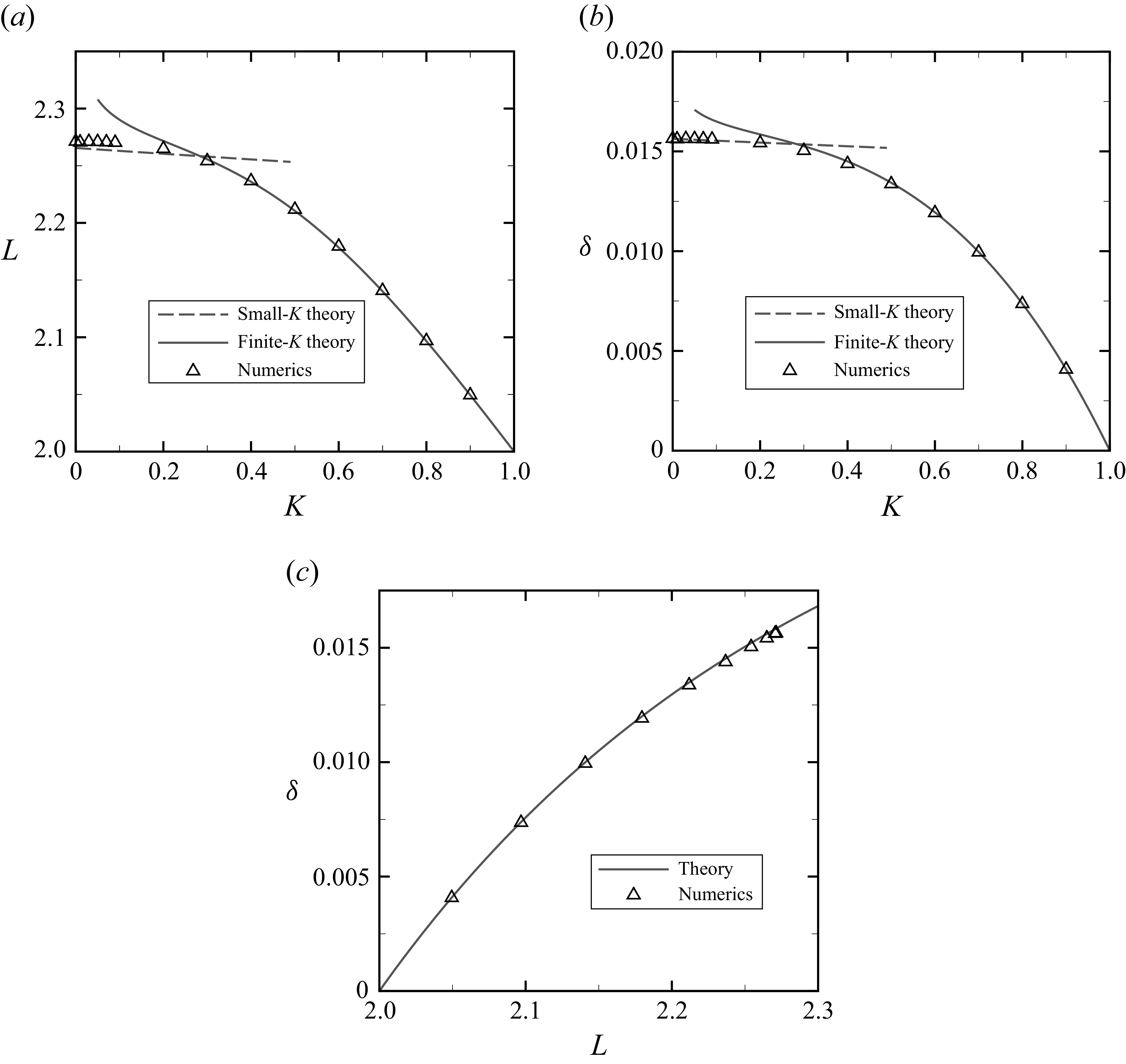
Comparison of the theoretical and numerical results during the steady migration stage. Variation of (a) the droplet length $L$ and (b) the migration velocity $\delta$ as a function of $K$ . The finite- $K$ theory corresponds to (3.14) and (3.15); the small- $K$ theory corresponds to (3.15) and (3.18). (c) Migration velocity $\delta$ as a function of $L$ with the theoretical curve given by (3.15).

Figure 3 compares the finite- $K$ and small- $K$ theories with numerical results of (3.2) and (3.3), which are obtained using the numerical approach described in Appendix A. As expected, the droplet becomes longer and moves faster at smaller $K$ since the driving force becomes stronger. The finite- $K$ theory shows excellent agreement with the numerical results for $K\gtrsim 0.2$ . For $K\lt 0.2$ , both $K$ and $\delta$ remain finite and are reasonably predicted by the small- $K$ theory, while the finite- $K$ theory fails. The dependence between $\delta$ and $L$ is shown in figure 3(c), in which the solid curve represents (3.15), valid for both finite and small values of $K$ as confirmed by the numerical solutions.

3.2. Asymmetric spreading

The migration stage ends when the receding contact line reaches the wettability border and hence all the liquid is accumulated on the more hydrophilic region of the substrate. At this instant, the apparent contact angle $\theta _0=4/L^2$ lies within the interval $(K,1)$ . Therefore, the droplet has yet to reach its equilibrium state on the more hydrophilic region. A further spreading process ensues until the apparent contact angle decreases to $K$ . During this stage, the advancing contact line keeps moving, and the other contact line is pinned at the border, leading to an asymmetric spreading.

The dynamics of the asymmetric spreading stage is governed by (3.1a ), while the BCs require appropriate treatment due to the presence of the pinned contact line. Different from the moving contact line, the contact angle is not known a priori at the pinned contact line and hence cannot be implemented as a BC. Instead, a zero-flux condition $h^2\,\partial _x^3h=0$ is adopted, and the BCs are

(3.19a,b) \begin{align} h=0,\quad h^2\partial _x^3h=0 \quad \text{at} \quad x=0, \\[-12pt]\nonumber \end{align}

(3.19c,d) \begin{align} h=0,\quad \partial _xh=-K \quad \text{at} \quad x=L. \end{align}

The contact line is therefore strictly pinned at $x=0$ , and the smoothed border (2.7) can be discarded. The volume conservation condition (3.4) can be used to fully determine the solution.

An asymptotic analysis can be performed as well when $\lambda \ll 1$ . It turns out that a boundary layer still occurs at the pinned contact line. The whole drop can thus be divided into an outer region and two inner regions near the contact lines. In the outer region, the slip term and the contact angle condition are neglected. For small spreading rate $\dot {L}$ , we seek an outer solution of the form

(3.20) \begin{equation} h(x,t)=h_0(x,L)+\dot L\,h_1(x,L)+\mathcal{O}(\dot L^2). \end{equation}

Accordingly, we have $\partial _t h=\dot L\,\partial _L h_0+\mathcal{O}(\dot {L}^2)$ . The leading-order governing equation and BCs are obtained as

(3.21a) \begin{gather} \partial _x\big (h_0^3\,\partial _{x}^{3}h_0\big )=0, \end{gather}

(3.21b) \begin{gather} h_0=0,\quad h_0^2\,\partial _x^3h_0=0 \quad \text{at} \quad x=0, \end{gather}

(3.21c) \begin{gather} h_0=0 \quad \text{at} \quad x=L, \end{gather}

(3.21d) \begin{gather} \int _{0}^{L}h_0\, \mathrm{d}x=\frac {2}{3}. \end{gather}

Integrating (3.21a ) once and using (3.21b ) yields $\partial _{x}^{3}h_0=0$ . Thus the leading-order solution again represents a hydrostatic profile:

(3.22) \begin{equation} h_0=\frac {4}{L^3}x(L-x). \end{equation}

The first-order solution $h_1$ satisfies

(3.23a) \begin{gather} \partial _L h_0+\partial _x\big (h_0^3\,\partial _x^3 h_1\big )=0, \end{gather}

(3.23b) \begin{gather} h_1=0,\quad 2h_0h_1\,\partial _x^3h_0+h_0^2\,\partial _x^3h_1=0 \quad \text{at} \quad x=0, \end{gather}

(3.23c) \begin{gather} h_1=0 \quad \text{at} \quad x=L, \end{gather}

(3.23d) \begin{gather} \int _{0}^{L}h_1\, \mathrm{d}x=0. \end{gather}

The solution can be found as

(3.24) \begin{equation} h_1=\frac {L^3}{32}\left [3x(L-x)+x^2\ln \frac {x}{L}+\big(L^2-x^2\big)\ln \left (\frac {L-x}{L}\right )\right ]\!. \end{equation}

The first-order derivative of $h_1$ diverges at $x=L$ , indicating the well-known singularity of moving contact lines. At the pinned contact line, $h_1$ has a finite slope, which can serve as a correction to the definition of the apparent contact angle:

(3.25) \begin{equation} \theta =\partial _xh_0(0)+\dot {L}\,\partial_xh_1(0)=\frac {4}{L^2}+\frac {L^4\dot L}{16}. \end{equation}

Interestingly, the second-order derivative still exhibits a logarithmic singularity, indicating the presence of a boundary layer at the pinned contact line.

The inner solution at the advancing contact line is given by (3.12) for finite $K$ , and by (3.17) for small $K$ , with contact line speed $\delta$ replaced by $\dot {L}$ . Matching these solutions with the cube of the derivative of the outer solution (3.20), we arrive at a reduced equation for the droplet width $L$ that, for finite $K$ , reads

(3.26) \begin{equation} \dot L=\frac {(2/L)^6-K^3}{3\ln (\textit{KL}/\mathrm{e}\lambda )}. \end{equation}

As the equilibrium state is approached, it has $\dot {L}\to 0$ and $L\to L_{eq}=2/\sqrt {K}$ . Equation (3.26) can be easily solved and validated against the numerical solution (which is introduced in Appendix B), as shown in figure 4, where the initial value of $L$ is given by the steady migration stage. The results show that a smaller value of $K$ leads to a faster contact line velocity, but prolongs the time to reach equilibrium. For small $K\to 0$ , the evolution of the droplet length is given by

(3.27) \begin{equation} \dot L\! \left (q+3\ln \frac {L\dot L^{1/3}}{\mathrm{e}\lambda }\right )-\left (\frac {2}{L}\right )^6=0, \end{equation}

where $q=0.74+K^2\dot L^{-2/3}$ . This relation is used to produce the theoretical curve of $K=0$ in figure 4. In this special case of complete wetting, the droplet spreads infinitely as no equilibrium state is expected. For small yet finite values of $K$ , we note that (3.27) does not hold when approaching the equilibrium state, because the contact line speed satisfies $\dot {L}\to 0$ , thereby violating the assumption $\dot {L}/K^3\gg 1$ required by (3.17). In this situation, one can adopt (3.26) to describe the very late stage of spreading, which, however, is out of the scope of the present work.

Figure 4.

Temporal evolution of the droplet length $L$ during the asymmetric spreading stage.

Besides the conditions of vanishing film thickness and flux, the derivation of the droplet evolution does not require any knowledge of the microscopic behaviour near the pinned contact line, implying that the local behaviour near the pinned contact line is determined by the macroscopic dynamics. Accordingly, the outer solution supplies a far-field condition for the inner region. We present an asymptotic analysis to elucidate the structure of the boundary layer near the pinned contact line, and demonstrate that the curvature singularity can be regularised by introducing the Navier slip. To this end, we introduce the inner variables

(3.28) \begin{equation} \xi =\frac {x}{\lambda },\quad H=\frac {h}{\lambda }. \end{equation}

The governing equation for the inner region becomes

(3.29) \begin{equation} \lambda\, \partial _t H+\partial _\xi \big [H^2(H+1)\,\partial _\xi ^3H\big]=0, \end{equation}

with BCs

(3.30) \begin{equation} H=0,\quad H^2\,\partial _\xi ^3H=0\quad \text{at} \quad \xi =0. \end{equation}

As $\xi \to \infty$ , we anticipate that the inner and outer solutions can be matched. Expressing (3.20) together with (3.22) and (3.24) in terms of the inner variables, and expanding for large $\xi$ , we obtain

(3.31) \begin{align} H\sim \frac {4\xi }{L^2}+\frac {L^4\xi }{16}\dot L-\frac {4\xi ^2}{L^3}\lambda +\frac {L^3\xi ^2}{32}\epsilon +\frac {L^3\xi ^2}{64}\left (2\ln \frac {\xi }{L}-7\right )\dot L\lambda +\cdots \quad \text{as} \quad \xi \to \infty , \end{align}

where $\epsilon \equiv \dot L\lambda \ln \lambda$ . This asymptotic relation serves as the far-field condition for the inner region.

Inspired by the form of (3.31), we consider a more general situation in which $\dot L$ , $\lambda$ and $\epsilon$ are independent and vanishingly small, and seek an inner expansion in the form

(3.32) \begin{equation} H(\xi ,t)=H_0(\xi ,L)+\dot L\,H_1(\xi ,L)+\lambda\, H_2(\xi ,L)+\epsilon\, H_3(\xi ,L)+\dot L\lambda\, H_4(\xi ,L)+\cdots . \end{equation}

Then the first term in (3.29) becomes

(3.33) \begin{equation} \lambda\, \partial _t H=\dot L\lambda\, \partial _L H_0+\cdots , \end{equation}

which allows the time derivative to be dropped up to order $\mathcal{O}(\dot L\lambda )$ . It is straightforward to successively demonstrate that

(3.34) \begin{equation} \partial _\xi \big [H_0^2(H_0+1)\,\partial _\xi ^3H_n\big ]=0 \end{equation}

for $n\in \{0,1,2,3\}$ , and

(3.35) \begin{equation} \partial _LH_0+\partial _\xi \big [H_0^2(H_0+1)\,\partial _\xi ^3H_4\big ]=0. \end{equation}

The BCs are obtained as

(3.36) \begin{equation} H_n=0,\quad H_0^2\,\partial _\xi ^3H_n=0\quad \text{at}\quad \xi =0, \end{equation}

for $n\in \{0,1,2,3,4\}$ , and

(3.37) \begin{equation} H_0\sim \frac {4}{L^2}\xi , \quad H_1\sim \frac {L^4}{16}\xi ,\quad H_2\sim -\frac {4}{L^3}\xi ^2 ,\quad H_3\sim \frac {L^3}{32}\xi ^2 ,\quad H_4\sim \frac {L^3\xi ^2}{64}\left (2\ln \frac {\xi }{L}-7\right )\!, \end{equation}

as $\xi \to \infty$ . The corresponding solutions can be found as

(3.38) \begin{gather} \begin{split} H_0=\frac {4}{L^2}\xi , \quad H_1=\frac {L^4}{16}\xi ,\quad H_2=-\frac {4}{L^3}\xi ^2+A\xi ,\quad H_3=\frac {L^3}{32}\xi ^2+B\xi ,\\ H_4=\frac {L^3}{512}\big [(L^2+4\xi )^2\ln (L^2+4\xi )-2L^4\ln {L}\big ]-\frac {2\ln (4L)+7}{64}L^3\xi ^2+C\xi . \end{split} \end{gather}

The coefficients $A$ , $B$ and $C$ remain to be determined; however, the corresponding terms only introduce an $\mathcal{O}(\lambda )$ correction of the film thickness and slope, and do not contribute to the curvature. Accordingly, the surface slope in terms of outer variables, after assigning $\epsilon =\dot L\lambda \ln \lambda$ , is given by

(3.39) \begin{equation} \partial _x h=\frac {4}{L^2}+\frac {L^4\dot L}{16}+\mathcal{O}(\lambda ), \end{equation}

which is consistent with (3.25) and hardly varies across the inner region near the pinned contact line. The second-order derivative has the form

(3.40) \begin{equation} \partial ^2_x h=\kappa _{\textit{ap}}+\frac {L^3\dot L}{16} \ln \frac {\lambda L^2+4x}{4\mathrm{e}^2L}, \end{equation}

where $\kappa _{\textit{ap}}=-{8}/{L^3}$ is the curvature of the leading-order approximation of the outer solution (3.22), namely the apparent curvature. In particular, the curvature has been regularised in the presence of slip, leading to a finite microscopic curvature at the contact line

(3.41) \begin{equation} \kappa _m=\kappa _{\textit{ap}}+\frac {L^3\dot L}{16} \ln \frac {\lambda L}{4\mathrm{e}^2}, \end{equation}

which is a counterpart of the well-known Cox–Voinov law for moving contact lines (Voinov Reference Voinov1976; Cox Reference Cox1986).

A comparison between the asymptotic theory and numerical results is presented in figure 5; the latter are obtained using the numerical method described in Appendix B. As shown in figure 5(a), the temporal decrease of the contact angle during spreading is accurately predicted by (3.39). The instantaneous profile of the film curvature is plotted in figure 5(b). It is shown that the outer solution well predicts the macroscopic variation of the curvature, but fails to capture the finite curvature upon approaching the pinned contact line within a distance of $\mathcal{O}(10\lambda )$ , where the inner solution is necessary to describe the microscopic curvature. The outer and inner solutions overlap in a region characterised by a logarithmic variation of the curvature.

Figure 5.

Microscopic properties of the inner region near the pinned contact line for $K=0.5$ . (a) Evolution of the contact angle $\partial _xh(0,t)$ with the theoretical curve given by (3.39). (b) Snapshot of the surface curvature $\partial ^2_xh(x,t)$ at $t=50$ . The outer solution represents the second-order derivative of (3.20) together with (3.22) and (3.24); the inner solution corresponds to (3.40).

4. The 3-D droplets

For 3-D cases, theoretical solutions are difficult to obtain; nonetheless, several quantitative features can be revealed by solving the 3-D problem (2.2)–(2.6) with the numerical method introduced in § 2. A symmetric condition has been imposed on the $y=0$ plane to reduce the computational cost. As illustrated in figure 6 for $K=0.2$ , the two-stage evolution observed in 2-D cases is also present for 3-D droplets. In the migration stage, the droplet traverses the wettability border. When the droplet completely leaves the less hydrophilic side, the asymmetric spreading stage begins, and the droplet evolves towards equilibrium on the more hydrophilic substrate. Different from spreading on homogeneous substrates, this process is constrained by the wettability border, where part of the contact line is pinned. The droplet eventually detaches from the border at equilibrium.

Figure 6.

Snapshots of a 3-D droplet driven by a chemical step with $K=0.2$ : (a–c) migration stage and (d–f) asymmetric spreading stage.

Figure 7.

Snapshots of the contact line position at different time instants for $K=0.2$ . The arrows indicate the direction of increasing time. (a,b) Migration stage, separated by the (a) absence and (b) presence of pinned contact lines at the wettability border. (c,d) Asymmetric spreading stage, separated by the (c) absence and (d) presence of receding contact lines. The dashed lines mark the wettability border.

More details of the droplet evolution can be inferred from the morphology of the contact line, as shown in figure 7. For clarity, the migration stage is further divided into two sub-stages, depending on whether pinned contact lines occur. For $t\lesssim 80$ (figure 7 a), the droplet is elongated and moves across the wettability border. The contact line recedes at the droplet tail on the less hydrophilic side, and advances in the more hydrophilic region as well as the less hydrophilic region near the border. At $t\approx 80$ , only a small fraction of the liquid is left on the less hydrophilic region, where the whole contact line recedes afterwards, while the contact line on the more hydrophilic region keeps advancing. Consequently, the mismatch of the contact line speed causes the occurrence of pinned contact line at the border, as shown in figure 7(b). The two segments of the pinned contact line extend and eventually connect when the droplet fully enters the more hydrophilic region at $t\approx 130$ , after which the asymmetric spreading stage starts. The asymmetric spreading is analogously divided into two sub-stages based on the direction of contact line movement. At the beginning of spreading (figure 7 c), the contact line advances, accompanied by a slight increase of the length of the pinned contact line. At later times (figure 7 d), the contact line near the border begins to recede. Eventually, the droplet detaches from the wettability border and approaches the equilibrium state at the more hydrophilic substrate, which corresponds to a circular contact line.

Figure 8.

Temporal evolution of droplet length $L$ and the $x$ -coordinate of the foremost point $x_2$ .

The temporal evolution of droplet length $L$ and the foremost contact line position $x_2$ is depicted in figure 8. The two curves for each $K$ merge, hence $L=x_2$ in the asymmetric spreading stage. During the migration stage, $x_2$ increases in an approximately linear manner, especially for small values of $K$ . The droplet length $L$ exhibits a non-monotonic variation in the migration stage, in contrast to the 2-D cases where a steady migration with a constant length is present. A remarkable decrease of $L$ can be observed before the onset of asymmetric spreading stage, leading to a minimum length even less than the initial diameter of the contact line. As can be inferred from figures 7(a,b), this is due to lateral wetting flow on the more hydrophilic region, which increases the longitudinal dewetting speed at the droplet rear. In the asymmetric spreading stage, the droplet length increases towards the equilibrium value.

The maximum droplet width on more hydrophilic region $W$ is plotted in figure 9 as a function of $t$ in log–log scales. The grey dots mark the critical instants between the two stages, which correspond to the instants when the leftmost point crosses $x=0$ , or equivalently to the merging points of $L$ and $x_2$ in figure 8. At early times, the maximum width occurs at the border and increases following the power law $W\sim t^{1/2}$ , reminiscent of the early growth of bridge width in the coalescence of sessile droplets (Ristenpart et al. Reference Ristenpart, McCalla, Roy and Stone2006; Kaneelil et al. Reference Kaneelil, Pahlavan, Xue and Stone2022). The increase of droplet width slows down over time. Interestingly, an overshoot is observed before approaching the equilibrium state. This is again associated with the lateral wetting flow once most of the liquid resides on the more hydrophilic region.

Figure 9.

Droplet width on the more hydrophilic side $W$ as a function of time. The grey dots mark the critical instants between two stages. The ratio of contact angles $K$ varies from 0.2 to 0.9 with increment 0.1. The equilibrium radius $R_{eq}$ is as marked for $K=0.2$ and $K=0.9$ .

5. Effect of initial condition

Figure 10.

The 2-D droplet length $L$ and the contact line positions $-x_1$ and $x_2$ as functions of (a) time $t$ and (b) the shifted time $\tau =t-t_0$ for $K_0\in \{1,1.5,2,3,5\}$ and $K=0.5$ . The grey dots mark the critical instants $t_0$ between the migration and asymmetric stages.

In this section, the effect of the initial droplet apparent contact angle $K_0$ is investigated by numerically solving the 2-D and 3-D problems. For both cases, the parameter $K_0$ is varied over the set $\{1,1.5,2,3,5\}$ , and the wettability contrast between two regions is fixed at $K=0.5$ . For ease of comparison, a shifted time $\tau =t-t_0$ is introduced, where $t_0$ is the critical instant between the migration stage and the asymmetric spreading stage. Droplet evolution with respect to both $t$ and $\tau$ is plotted and described below.

Figure 10 depicts the temporal variation of the contact line positions $x_1$ , $x_2$ and the length $L=x_2-x_1$ of 2-D droplets. Regardless of the initial apparent contact angle, the droplet always evolves into a stage of steady migration, followed by a stage of asymmetric spreading. The steady migration and the asymmetric spreading are preceded by an early spreading that elongates the droplet to the same length, which is determined by $K$ as obtained in § 3.1. After reaching the same steady migration state, the subsequent droplet motions are identical, as demonstrated in figure 10(b) by using the shifted time $\tau$ . The differences are only evident in the early spreading process before approaching the steady state. For the case $K_0=1$ , the droplet advances only on the more hydrophilic region, and recedes on the less hydrophilic region, whereas for $K_0\gt 1$ , the droplets initially spread simultaneously on both sides, as indicated by the non-monotonic variation of $x_1$ . As $K_0$ increases, the droplet is more plump upon contact with the wettability border, hence both contact lines advance more rapidly, and the elongation accelerates, causing a faster early spreading. The transient advancing of the left-hand contact line is reversed by the overwhelming effect of the wettability contrast and the steady migration develops. As the droplet at larger $K_0$ is narrower, it leaves the less hydrophilic region at an earlier time $t_0$ .

Figure 11.

The 3-D droplet size and position as functions of (a,c) time $t$ and (b,d) shifted time $\tau$ under different $K_0\in \{1,1.5,2,3,5\}$ and fixed $K=0.5$ . (a,b) Droplet length $L$ and the $x$ -coordinates of the backmost point $x_1$ and the foremost point $x_2$ . (c) Droplet width $W$ in log–log coordinates. (d) Droplet width $W$ as a function of shifted time $\tau$ in linear coordinates. The grey dots mark the critical instants $t_0$ between the migration and asymmetric stages.

For 3-D droplets shown in figure 11, the effect of $K_0$ is also confined to the early process. Figures 11(a,b) demonstrate the droplet evolution along the $x$ -direction, where the length varies non-monotonically during migration, but qualitatively similar $K_0$ -dependence in the 2-D cases is observed. For different $K_0$ , the droplet length and $x$ -coordinates still converge at some point and follow the same dynamics thereafter when the shifted time is used. The droplet width $W$ defined in the $y$ -direction, shown in figures 11(c,d), grows more rapidly for larger $K_0$ in the early spreading process, but eventually converges during the migration stage before $\tau =0$ . When $K_0\gt 1$ , the $t^{1/2}$ law of the droplet width $W$ is violated at early times, presumably owing to the significant spreading on both regions.

As demonstrated above, the value of $K_0$ mainly influences the early spreading process that adjusts the droplet profile to reach the migration state, after which the evolution is determined by $K$ rather than $K_0$ .