Generalized Linear Models and probit analysis

In statistical terms, a linear model (LM) is one in which a response variable, Y, depends on one or more explanatory variables, X ₁, X ₂,…, X _p, through a single multiplicative parameter associated with each variable (i.e. the contribution of each explanatory variable to the response is obtained by multiplying the value of the variable by the respective parameter value). Simple linear regression analysis fits the simplest form of LM, where there is just one explanatory variable, and the model can be described by the equation

where y _i is the ith value of the response variable, x _i is the corresponding value of the explanatory variable, β₀ is the value of the response variable when the explanatory variable has value zero (the intercept), β₁ is the multiplicative parameter for the explanatory variable, and the random component of the model, the error term, ɛ_i, is assumed to follow a normal distribution with mean 0 and variance σ². Hence, the expectation of observation y _i given the value of the explanatory variable, x _i,

Multiple linear regression analysis extends this to include more than one explanatory variable, with the LM described by the equation

and the expected value of observation y _i, given the values of the p explanatory variables,

For a linear model, estimation of the parameters $$\beta _{o},\ldots , \beta _{p} $$ (p ≥  1) is achieved by minimizing the sum of the squared differences between observed and fitted values (the residual sum of squares) using the least squares algorithm (Sokal and Rohlf, Reference Sokal and Rohlf2012).

GLMs provide a relaxation of the assumption about the distribution of the errors following a normal distribution, a key element of the LM. This allows the use of other distributions in the exponential family, including the binomial distribution that is commonly associated with data in the form of proportions based on counts. In a GLM there is still a variable, η, now known as the ‘predictor’, that depends on one or more explanatory variables according to a linear relationship, such that the expected value of the predictor, given the values of the p explanatory variables,

The predictor is then related to the response variable through a ‘link’ function, g(.), such that g(μ_i) = η_i. In the case of probit analysis, an example of a GLM used for modelling proportions arising from a binomial response variable, the link function was originally the inverse of the cumulative normal distribution function, Φ^− 1. Applying the inverse link transformation to the predictor then allows that the expected proportion of successes, μ_i can take any value between 0 and 1:

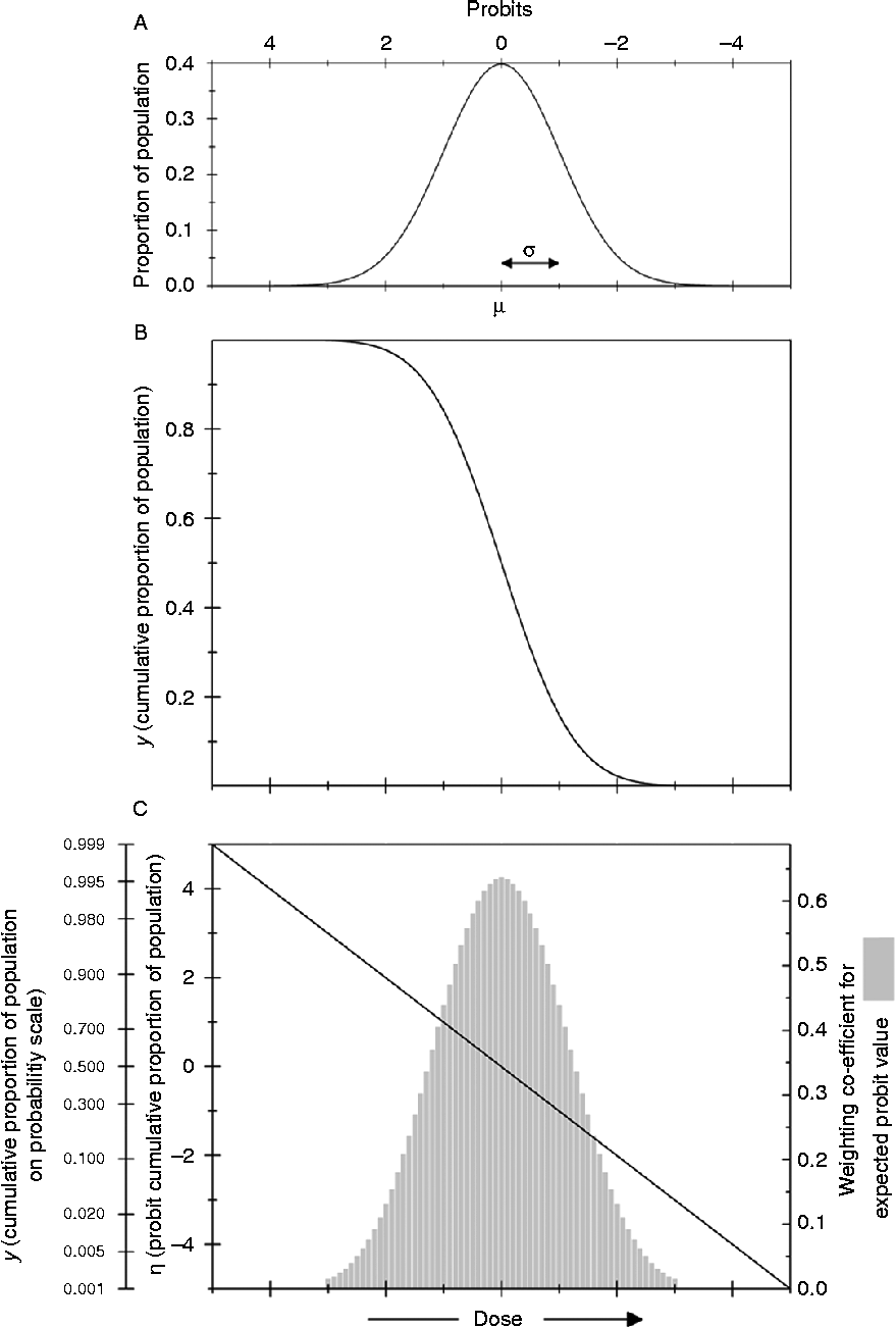
The implementation of the inverse cumulative normal distribution (probit) link function implies that the values of the explanatory variable at which individuals respond follow a normal distribution. Applying the inverse cumulative normal distribution function, Φ^− 1, to μ_i is essentially equivalent to carrying out a ‘probit transformation’ whereby proportions are ‘manually’ converted to probits (Fig. 1) prior to fitting a linear relationship, though in fitting a GLM the transformation is applied within the model rather than to the data. The probit linear predictor, η_i, can theoretically take any value between − ∞ and +∞; however, in probit transformation tables, the range of the probit linear predictor scale is typically given as between − 3.719 (proportion of successes = 0.0001) and +3.719 (proportion of successes = 0.9999). Historically, for computational ease, values were coded by addition of 5 (i.e. to lie between 1.281 and 8.719), making the range entirely positive. Using the former range, scale units may be called probits or normal equivalent deviates (NED); with the positive range, the units are invariably called probits.

Figure 1

The normal distribution and probit analysis. In the case of the seed viability equation in which ‘dose’ is the period of time in storage, there is a normal distribution of seed deaths over time (A) giving rise to a negative cumulative normal distribution where y is the proportion of viable seeds within the population (ability to germinate; B). Transforming y to the linear predictor η using the cumulative normal distribution function, i.e. by plotting germination against time using the probit scale shown at the top of (A), the curve becomes linear (C). Also shown in (A) is the mean (μ) and standard deviation (σ) of the normal distribution and in (C) the probability scale for the proportion of viable seeds in the population and the weighting coefficient for the expected probit value. More weight is given to probit values close to 0.

Derived from the binomial distribution, the variance of a proportion, p, (given by np(1–p), where n is the sample size) depends on the mean (given by np) and hence the process of fitting a probit GLM (equation 6) is weighted, with a higher weighting coefficient (smaller weight) for expected probit values that are closer to 0 NED, the middle of the response range (Fig. 1C). The actual weighting depends on both this weighting coefficient and the number of individuals used to determine the proportion of successes; the weight increases as n increases. Probit analysis therefore requires data on both the number of successes and the number of individuals tested.

To fit a GLM, statistical software uses an iterative process of parameter value setting (with initial parameter values estimated from the observed data), until there is convergence, where further changes in the parameter values do not improve the likelihood of obtaining the observed set of data, given the error associated with those observations (maximum likelihood estimation; McCullagh and Nelder, Reference McCullagh and Nelder1989). This process is exactly equivalent to the least squares algorithm where errors are assumed to follow a normal distribution. In equations (5) and (6), the parameter β₀ is the intercept value on the probit scale and the other parameters, β₁,…,β_p, describe the effect of the p explanatory variables on the probit proportion response. The reciprocals of these multiplicative parameters are then estimates of the standard deviations of the normal distribution of the process being followed in response to each explanatory variable.

For a linear model, the importance of each explanatory variable is assessed by calculating the change in the residual sum of squares when adding or dropping the variable from the model, with statistical significance determined by an F-test as summarized using analysis of variance (ANOVA). For a GLM, the importance of each explanatory variable can be similarly assessed by calculating the change in the residual deviance, equivalent to the difference in the likelihood of the data given the models with and without the explanatory variable of interest. This is summarized in an analysis of deviance, with the statistical significance associated with the inclusion of each explanatory variable determined by a chi-squared test if the errors follow a binomial distribution. If the errors are larger than is expected for a binomial distribution (known as over-dispersion), statistical significance is determined using an approximate F-test (McCullagh and Nelder, Reference McCullagh and Nelder1989).

The pattern of departure of the observed values from a fitted model can be used to evaluate the goodness of fit of that model. For a linear model the errors can be estimated from the fitted model by calculating the raw residuals, r _i =  y _i −  μ_i (where μ_i is the fitted value), which are then standardized by dividing by their standard deviation. Plotting these standardized residuals against the fitted values of the response variable will then show any systematic departure of the observed data from the fitted model. Further plots of the standardized residuals allow visual assessment of the conformity to distributional assumptions. For a GLM, the calculated standardized residuals have to also take into account that the standard deviation of a proportion varies; deviance and Pearson residuals are suggested to provide appropriate correction (Pierce and Schafer, Reference Pierce and Schafer1986; McCullagh and Nelder, Reference McCullagh and Nelder1989) and can then be used similarly for model evaluation.

The use of the term ‘probit analysis’ has been broadened to cover any GLM that assumes a binomial error distribution and an appropriate link function (other commonly used functions are the logit and complementary log-log) that assumes a different distribution for the values of the explanatory variable at which individuals respond. These models may also be known as logit or logistic regression analysis and applied to analyse data from experiments with non-continuous explanatory variables (such as from an experiment with a factorial treatment structure). Where the design of an experiment is more complex, it may be necessary to apply a Generalized Linear Mixed Model (GLMM) analysis (Lee et al., Reference Lee, Nelder and Pawitan2006; Bolker et al., Reference Bolker, Brooks, Clark, Geange, Poulsen, Stevens and White2009).

Time to response models and survival analysis

Where the proportions of seeds responding (germinating) are collected as cumulative counts from a single sample, rather than as counts from independent (separate) samples, at each observation time, then the standard GLM assumption of independent observations is not satisfied and an alternative form of analysis should be used. In an extreme case of such data it might be possible to observe the exact time of response (germination) of each individual seed, providing a set of observations of the time to response. A more likely scenario, however, is that each sample will be observed at regular intervals (e.g. every 12 or 24 h, depending on the overall rate of response) so that the observed data are actually the numbers of seeds responding in each period of time. While the exact time of response for each individual is not known in this scenario, the data do provide information about the distribution of times to response, and should be analysed on this basis, rather than as the cumulative number (or proportion) responding.

With data in the form of either the individual times to response or the number of responses in each successive period of time, then the method of survival analysis, widely used in medical research and industrial applications, would be appropriate. Various models for the distribution of survival times (corresponding to the germination times) for individuals in a population have been proposed and are widely used (Cox and Oakes, Reference Cox and Oakes1984). These models include the exponential distribution, gamma distribution, Weibull distribution, log-normal distribution and log-logistic distribution. In the language of survival analysis, the survivor function represents the probability that the time to response (survival or germination) for an individual will exceed any given time (essentially the complement of the cumulative distribution function), with an associated probability density function given by, for example, one of the distributions identified above. Models are then often expressed in terms of the hazard function, also referred to as the age-specific failure rate. This is effectively the probability of response at any given point in time, given that response has not yet occurred. Associated with this hazard function is the integrated hazard, also referred to as the cumulative hazard as it is an accumulation of the hazard (the probability of response) over time. Formulae for these different functions can be derived for each of the distributions identified above, the exponential distribution providing the simplest form of hazard function with the hazard remaining constant, reflecting the so-called ‘lack of memory’ property of the exponential distribution.

A common issue, particularly in medical trials, is that of right-censored observations – where individuals drop out of the study before reaching the defined endpoint. For seed germination, where a study might be stopped after some pre-defined period of time, this concept relates to seeds that have not germinated by that pre-determined time. Of course, without further experimentation, such as viability testing under ideal conditions, it is impossible to know whether these non-germinated seeds have not yet reached their germination time or are unable to ever germinate. The issue of censoring in seed germination studies is somewhat different to that encountered in other applications of survival analysis, as censoring will generally be related to the maximum observation time. If the proportion of censored observations is large, then choice of the survivor function (underlying distribution of times to response) may have a significant impact on any summary statistics (such as the mean germination time or time to 50% germination) subsequently estimated from the fitted model.

A further form of censoring, extremely common for the data that are collected in germination studies, is interval censoring. As identified above, this is when it is known that the response occurred after one observation time and before a later observation time, so that the data record the number of responses between each pair of successive observation times, but the exact time at which the response occurred is not known. Clearly this introduces more uncertainty into the estimation of model parameters.

Survival models are generally fitted using a maximum likelihood approach, where the likelihood function is made more complicated by the need to consider censored observations. Rather than being able to consider the probability associated with each individual time to response, we have to consider the probability of response times within an interval (for interval censored data) or being greater than the maximum observation time (for right-censored data). Of course, identifying an appropriate survivor function to fit to the data is an important first step. Knowledge of the shapes of survivor functions can be combined with empirical estimates of the hazard at different observation times to aid in this identification. The Kaplan–Meier estimator (Kaplan and Meier, Reference Kaplan and Meier1958), or product limit estimator, provides an estimate of the survivor function as the product of the probabilities of survival (non-germination) across all prior observation times. Here the probability of survival is simply calculated as the number of individuals surviving prior to the observation time as a proportion of the number of individuals just prior to that time. This is probably more easily understood when considering interval censored data: the probability of survival at the end of each interval is the number of survivors at the end of the interval as a proportion of the number of survivors at the start of the interval. The empirical hazard for each time-point can also be calculated in this way and compared with the expected pattern for different distribution models.

Where there are multiple treatments to be considered (e.g. different species or cultivars or temperatures or water potentials, in seed germination studies), a number of approaches have been developed within survival analysis for comparing the survival responses under these different conditions. These include the accelerated life model, in which the time to a particular level of survival in one treatment is a constant multiple of the time in another treatment, and the proportional hazards model, in which the hazard function for one treatment is a constant multiple of the hazard for another treatment. Of course, the form that these relationships take will depend on the particular form of distribution chosen for the survivor function, and, again, plotting of empirical estimates of the survival or hazard functions, as described above, will help in the identification of an appropriate approach to compare treatments. While this approach is usually considered for qualitative treatment sets, the same approach can be extended to cope with quantitative treatment factors, such as dose or temperature.

Where data are only available in terms of the number of seeds that have germinated in successive intervals of time, an alternative analysis approach is to directly model the distribution of times to germination based on these grouped counts. This approach requires the use of a general (non-linear) regression/optimization approach, directly comparing the observed counts in each interval with the predicted counts according to some (statistical) distribution model, and using an optimization process to find the parameter values that most closely match the predicted counts to the observed counts. The modelling process assumes a multinomial distribution for the counts of germination events in the set of observed intervals, and can be fitted using either a generalized least squares approach or a maximum likelihood approach (the preferred approach; see Hunter et al., Reference Hunter, Glasbey and Naylor1984; Brain and Butler, Reference Brain and Butler1988; and others). This approach allows almost any distribution function to be used to describe the observed distribution of germination counts and enables distributions to be fitted simultaneously to responses for multiple treatments by allowing the parameters of the distribution to be expressed as functions of the treatments (e.g. temperature or water potential), something that is much more difficult within the survival analysis approach (but for one approach, see Manso et al., Reference Manso, Fortin, Calama and Pardos2013).

Loss of ability to germinate

Using data from cereal seed storage and by plotting percentage germination on a probability scale (the equivalent of converting percentage values into probits; Fig. 1), it was observed that the distribution of seed deaths over time in storage (in a constant environment) is approximately normal (the distribution may be slightly skewed when there is very rapid loss of viability) (Roberts, Reference Roberts1960). This finding, together with consideration of the effect of moisture content and temperature on the half-viability period (the time for viability to fall to 50%, p ₅₀), led to the first version of the seed viability equation for describing seed survival curves in a given (constant) storage environment.

Expressing the Ellis and Roberts (Reference Ellis and Roberts1980a) improved viability equation as a GLM, the proportion of seeds, y, that have the ability to germinate after a given period of storage is given by

The link function, Φ^− 1, is the inverse of the cumulative normal distribution function; the linear predictor is designated by v (probit viability); and the explanatory variable by p (period of storage under constant conditions). More familiarly, this may be expressed in probits as

The parameters to be estimated through probit analysis are the theoretical viability of the seeds when they are placed into storage, K _i (‘β₀’ in equation 6) and the parameter describing the effect of storage period on germination, − σ^− 1 (‘β₁’ in equation 6). In this model, σ is the standard deviation of the normal distribution of seed deaths in time (Fig. 1A), i.e. the period of time for viability to fall by 1 probit (Fig. 1C). Data are entered as columns of storage period, number of seeds that germinate and number of seeds sown. It does not matter if the number of seeds sown after different periods of storage varies; for example, if seeds are aged in packets and there happens to be a few more seeds in some packets compared with others, it might be better to sow all the seeds from each packet anyway, rather than risk any non-random selection when taking seeds from the packet. Nor does it matter whether the seeds from each packet are sown as one lot (e.g. in one Petri dish) or multiple lots (in multiple Petri dishes), though the total germination across multiple Petri dishes from the same packet should be recorded as a single observation. Where replicate packets are available for a particular treatment, then the data from each packet should be recorded separately (i.e. three replicate packets results in three separate estimates of the proportion germinated for that treatment).

As well as providing estimates for K _i and σ, the probit analysis procedure can generate an estimate (and the standard error of that estimate) of the time for viability to fall to 50% (p ₅₀), or indeed any other ‘lethal dose’. The p ₅₀ is both the mean and median for the normal distribution of times to seed death. Where initial viability is less than 50%, or the final viability is greater than 50%, the p ₅₀ will be estimated from the extrapolation of the fitted model. This will lead to a negative estimate of p ₅₀ in the former case. The viability in probits is 0 when there is 50% germination. Hence,

and p ₅₀=  K _i ×  σ. Estimates of p ₅₀ from probit analysis of seed storage data have been used to compare the longevity of different seed-lots (e.g. Hay et al., Reference Hay, Klin and Probert2006) or of seeds from different species (e.g. Zewdie and Ellis, Reference Zewdie and Ellis1991; Probert et al., Reference Probert, Daws and Hay2009). It should be emphasized that p ₅₀ takes into account possible variation in both K _i and σ between seed-lots; it is not a direct measure of the rate of (probit) viability loss but also reflects the initial quality of the seeds. For broad comparisons of relative seed longevity, across species for example, it may be preferable to control for variation in initial seed quality that may be due to, for example, differences in seed maturity or processing, by only using seed-lots with similar initial germination, as adopted by Probert et al. (Reference Probert, Daws and Hay2009), or to use σ as the measure of relative seed longevity.

In special cases, apparent when the observed survival curve is asymmetric, a proportion of the seeds placed into storage are not part of the ageing population and it may be appropriate to include an additional ‘control viability’ parameter, C _v, for estimation in the probit analysis (Mead and Gray, Reference Mead and Gray1999):

When C _v = 1, all the seeds are part of the ageing population; when C _v< 1, there are two classes of dead seeds, those that were part of the ageing population at p =0 and have already lost viability, which is reflected in low K _i, and those that were not part of the ageing population of seeds but were ‘non-respondents’ for some other reason. For example, in theory, if a consistent proportion of seeds remained dormant throughout a storage experiment, C _v would be < 1. C _v therefore estimates the size of the responding ageing population as a proportion of the total population. This additional parameter has been found to be particularly useful in modelling the survival curves of seeds that have been pre-aged, primed and then returned to storage, where there were significant proportions of seeds that were non-responders (Butler et al., Reference Butler, Hay, Ellis, Smith and Murray2009; Wood and Hay, Reference Wood and Hay2010).

Ellis and Roberts (Reference Ellis and Roberts1980a, Reference Ellis and Robertsb) went on to describe how the value of σ varied depending on the moisture content, m% fresh weight, and temperature, t°C, during storage. Through a series of regression analyses of σ against moisture content and temperature, the following equation was derived:

Combining equations (10) and (11),

Using current statistical software it is possible to determine all the unknown parameters in this equation through a ‘one-step’ analysis of the data from multiple storage environments (Hay et al., Reference Hay, Mead, Manger and Wilson2003; Demir et al., Reference Demir, Kenanoglu, Hay, Mavi and Celikko2011; Crawford et al., Reference Crawford, Hay, Plummer, Probert and Steadman2013): K _i as the GLM β₀ parameter; K _E, C _W, C _H, and C _Q as part of the estimation of the GLM β₁ parameter, − σ^− 1; and C _v as the responding proportion of the population. For example, in GenStat (VSN International, UK) this is done using the FITNONLINEAR directive (Payne et al., Reference Payne, Harding, Murray, Soutar, Baird, Glaser, Welham, Gilmour, Thompson and Webster2011). Data are entered as columns of storage temperature, storage moisture content, storage period, number of seeds that germinate and number of seeds sown. As discussed by Hay et al. (Reference Hay, Mead, Manger and Wilson2003), this one-step approach takes into account all the variability in the data and it is not necessary to have a complete factorial design whereby seeds are stored at all combinations of target moisture contents and temperatures. It is also possible to test statistically whether or not any or all of the parameters vary between seed-lots or, for example, whether the parameters C _H and C _Q differ from the so-called ‘universal values’ (Dickie et al., Reference Dickie, Ellis, Kraak, Ryder and Tompsett1990), as was found using this one-step approach for two ecotypes of Arabidopsis thaliana L. (Hay et al., Reference Hay, Mead, Manger and Wilson2003).

As discussed elsewhere (Pritchard and Dickie, Reference Pritchard, Dickie, Smith, Dickie, Linington, Pritchard and Probert2003), probit-based modelling of seed survival curves is not always favoured. Alternative models that have been considered include the Gompertz equation (Bernal-Lugo and Leopold, Reference Bernal-Lugo and Leopold1998), Avrami kinetics (Walters, Reference Walters1998; Walters et al., Reference Walters, Wheeler and Grotenhuis2005) and others (Hundertmark et al., Reference Hundertmark, Buitink, Leprince and Hincha2011), fitted to germination proportion data. Indeed, there are many equations that describe a sigmoidal curve. In contrast to probit analysis, however, such models do not take into account the binomial errors associated with measuring percentage germination, and therefore may not apply the appropriate weighting to different observations in estimating the model parameters. The binomial error assumption could be combined with these alternative models by identifying appropriately shaped link functions. For example, the asymmetric curve described by the Gompertz equation can be approximated within a binomial GLM by using the complementary log-log link function. Where an appropriate link function can be identified, modifications of the ‘one-step’ analysis approach developed by Hay et al. (Reference Hay, Mead, Manger and Wilson2003) will provide parameter estimates that take full account of the binomial error structure of the germination count data, and the effects on the viability response of different environmental storage treatments.

Seed germination progress curves

As previously identified, the data in germination studies are usually recorded as cumulative proportions of germinated seeds for each sample at successive observation times. Although these data do not satisfy the usual assumption of independence associated with regression analysis against a continuous explanatory variable, cumulative proportions have often been transformed to probits prior to linear regression analysis, or probit analysis applied to the cumulative counts (from which the proportions have been derived). If experiments were designed so that successive observations were made on independent samples of seed, then these analysis approaches would be entirely valid. This would require considerably more seeds than used in current practice, so, for example, in a study looking at the effects of different temperatures on seed germination, a separate sample of seeds would need to be sown at each temperature for each planned observation time (i.e. each Petri dish of seeds would be observed once and then discarded). It would then be possible to follow a probit analysis approach to the fitting of germination progress models, for example, thermal time, hydrotime, hydrothermal time and other threshold-based models.

Bradford (Reference Bradford, Kigel and Galili1995) acknowledged that ‘… proper application of probit analysis requires that the samples at each time point be independent (Finney, Reference Finney1971)’, but concluded that the observed germination data would be the same whether collected from dependent or independent samples, and therefore that the probit analysis approach was valid. However, failure to take into account the non-independence of successive cumulative counts results in an underestimation of the underlying error, such that differences between treatments will be more likely to appear statistically significant (Hunter et al., Reference Hunter, Glasbey and Naylor1984). Although often we do not appear to be directly interested in tests of differences in parameter values between treatments (but rather in identifying the best-fitting model), the simultaneous fitting of models across different environmental conditions does involve the comparison of the (probit) slope and intercept parameters between treatments when modelling these parameters as functions of the environmental conditions, and hence some formal assessment of these differences. Further, assessment of the need to add an extra parameter to the model effectively involves the assessment of whether that extra parameter is different from zero. In addition to the underestimation of the error, there is evidence (Mesgaran et al., Reference Mesgaran, Mashhadi, Alizadeh, Hunt, Young and Cousens2013, online appendix C) that model fitting to cumulative data results in an overestimation of the cumulative germination at any time-point relative to the ‘correct’ model fitting to non-cumulative counts, probably as a result of the cumulative errors associated with the cumulative count data.

The ideal probit analysis fitting process for these germination progress models is described below for a range of different model scenarios, assuming that the data are collected from independent samples at the different observation times (to illustrate the theoretical approach, though the example data used are generally based on cumulative observations). However, given that non-independent cumulative data are more commonly collected, appropriate alternative approaches, based on time-to-response or survival models, are then identified, allowing the application of a wide range of distribution functions for the times to germination (not just the normal distribution). Hunter et al. (Reference Hunter, Glasbey and Naylor1984) appear to be the first to have developed such a model for the distribution of times to germination rather than for the cumulative germination to a particular time-point. Their model is based on assuming that these times followed a normal distribution, possibly after some suitable transformation.

Germination over time

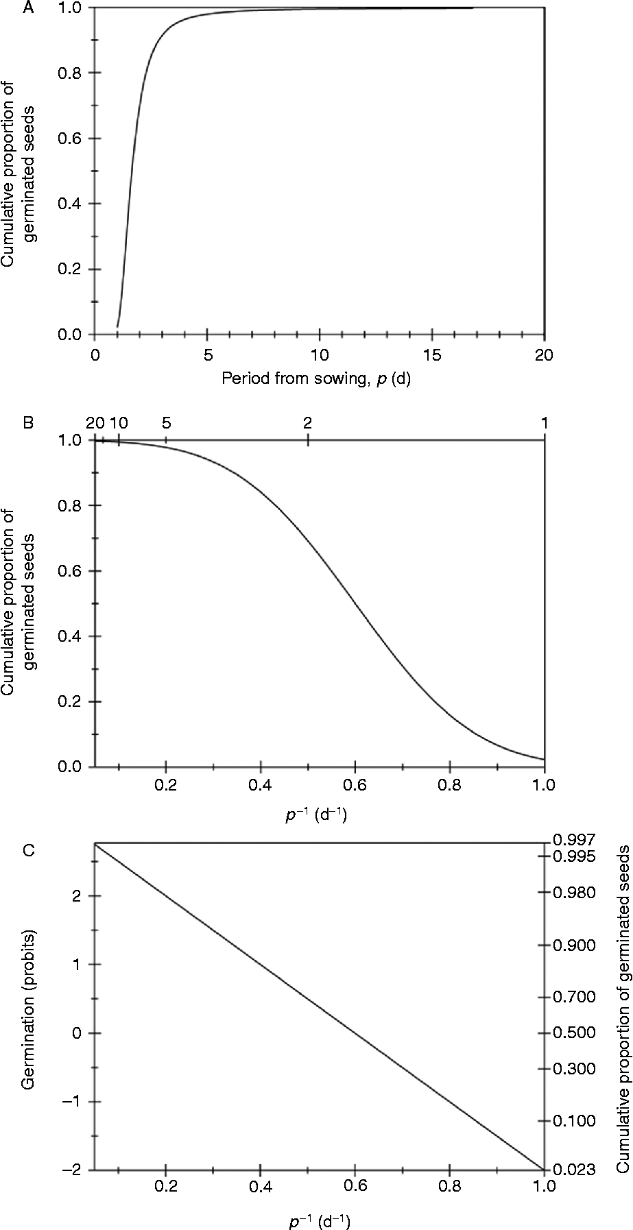
The cumulative germination time course for a population of non-dormant seeds often follows a broadly sigmoidal shape, so that it might be a natural assumption that the times to germination follow a normal distribution (Janssen, Reference Janssen1973) and so could be modelled using the cumulative normal distribution curve. However, the germination progress curves are often not symmetrical, since the rate of increase in cumulative germination slows over time; a variety of other models (e.g. logistic curve, four-parameter Hill function) and/or cumulative statistical distribution curves (e.g. Weibull, log-normal, negative exponential) have therefore been used to describe germination progress (Scott et al., Reference Scott, Jones and Williams1984; Dumur et al., Reference Dumur, Pilbeam and Craigon1990; Roman et al., Reference Roman, Thomas, Murphy and Swanton1999; O'Neill et al., Reference O'Neill, Thomson, Jacobs, Brain, Butler, Turner and Mitakda2004; El-Kassaby et al., Reference El-Kassaby, Moss, Kolotelo and Stoehr2008). This asymmetry has also been accommodated by plotting the germination proportion against the logarithm (Scott and Jones, Reference Scott and Jones1985; Dahal et al., Reference Dahal, Bradford and Jones1990) or reciprocal (Campbell and Sorensen, Reference Campbell and Sorensen1979) of the period of time from sowing, enabling the fitting of a cumulative normal distribution curve with a positive (not shown) or negative (Fig. 2) slope, respectively.

Figure 2

The use of probit analysis to describe germination progress curves. The cumulative proportion of seeds germinating, plotted (A) against period of time from sowing, p; and (B) against p ^− 1 (bottom axis) and p (top axis, reciprocal scale). Note that in (B) the curve has become symmetrical about 50%. Transforming the proportion of seeds that germinate to probit values results in a linear relationship with p ^− 1 (C). Also shown in (C) is the probability scale for the proportion of seeds that germinate.

Where the explanatory variable (e.g. time to germination, logarithm of time to germination, reciprocal of time to germination) is assumed to follow a normal distribution, then a probit analysis approach would be appropriate, with the respective GLMs expressed as

where g is germination as a proportion of the seeds sown; γ is the linear predictor, i.e. germination in probits; β₀ is the maximum germination in probits; and β₁ describes the rate of increase (13a,b) or decrease (13c) in probit germination as the explanatory variable (p, ln(p) or p ^− 1) increases. The reciprocal of time from sowing is often referred to as ‘germination rate’ (GR), although here it will generally be referred to as p ^− 1 (inverse of the period of time from sowing) since it is not a true rate (i.e. number of additional seeds that germinated over a unit of time). Data are entered as before – the explanatory variable, number of seeds that germinate and number of seeds that are sown. Interpretation of the fitted model in terms of the distribution of times to germination for individual seeds is not straightforward for the latter two models. The analysis can estimate the value of the explanatory variable associated with achieving 50% germination; the time associated with achieving 50% germination can easily be obtained from this value, but this is not the mean time to germination, since the time to germination is not normally distributed (the distribution is not even symmetric, as illustrated in Fig. 2 with p ^− 1 as the explanatory variable). Rather, it is correctly referred to as the median germination time. Other percentiles of the germination time distribution can be similarly estimated from the fitted model.

Thermal time

The effect of temperature on seed germination has long been of interest. Seeds of different species germinate over different temperature ranges, as exemplified by experiments using thermal gradient plates (e.g. Ellis et al., Reference Ellis, Hong and Roberts1983; Chejara et al., Reference Chejara, Kristiansen, Whalley, Sindel and Nadolny2008; Zhang et al., Reference Zhang, McGill, Irving, Kemp and Zhou2013). So-called ‘cardinal temperatures’ have been defined as the minimum or base temperature, T _min or T _b, below which no seeds germinate; the maximum or ceiling temperature, T _max or T _c, above which no seeds germinate; and either a single optimum temperature, T _opt, or an optimum temperature range where maximum percentage germination is observed (e.g. Garcia-Huidobro et al., Reference Garcia-Huidobro, Monteith and Squire1982; Ellis et al., Reference Ellis, Covell, Roberts and Summerfield1986; Shafii and Price, Reference Shafii and Price2001; Hardegree, Reference Hardegree2006; Naylor, Reference Naylor2007; Zhang et al., Reference Zhang, McGill, Irving, Kemp and Zhou2013).

At sub-optimal temperatures, between T _b and T _opt, the rate of germination increases with temperature. This has been described in terms of the accumulated thermal time, θ_T(g), above T _b required for a specified percentage, g, of the population to germinate. This can be expressed using the equation

where GR _g (indicating ‘germination rate’) is the reciprocal of the period of time, p, to reach g% germination, T is the constant temperature to which the seeds are exposed and T _b(g) is the base temperature for the germination of the gth percentile of the population (Garcia-Huidobro et al., Reference Garcia-Huidobro, Monteith and Squire1982).

The base temperature, T _b, has typically been determined through linear regression analysis of GR (hereafter referred to as p ^− 1(g); see above) against temperature, for a single value of g% germination (usually 50%) or for a range of values of g (e.g. 10, 20,…, 90). The values of p ^− 1(g) are generally estimated through interpolation of germination progress curves (e.g. Covell et al., Reference Covell, Ellis, Roberts and Summerfield1986). Using a range of values of g, Garcia-Huidobro et al. (Reference Garcia-Huidobro, Monteith and Squire1982) found that T _b varied by a few degrees within a seed-lot of pearl millet. Others, including Covell et al. (Reference Covell, Ellis, Roberts and Summerfield1986), Ellis et al. (Reference Ellis, Covell, Roberts and Summerfield1986, Reference Ellis, Simon and Covell1987), Dahal et al. (Reference Dahal, Bradford and Jones1990) and Crauford et al. (Reference Crauford, Ellis, Summerfield and Menin1996), noting that regression lines for different percentiles appeared to converge, constrained the regression lines to have the same intercept on the temperature (horizontal) axis. While other authors (Garcia-Huidobro et al., Reference Garcia-Huidobro, Monteith and Squire1982; Kebreab and Murdoch, 1999b) report some variation in values of T _b within seed populations, almost all studies of seed germination based on thermal time assume a single value of T _b for the entire seed population, often with verification of this assumption by plotting p ^− 1(g) against temperature for different values of g.

Having determined a constant value of T _b by constraining the regression lines of p ^− 1(g) against temperature, for g= 10, 20, 30,…, 90% germination, Ellis et al. (Reference Ellis, Covell, Roberts and Summerfield1986) found that there was a sigmoidal relationship between cumulative percentage germination and thermal time, p· (T – T _b); they concluded that the amount of thermal time individual seeds needed to accumulate in order to germinate followed a normal distribution. Hence, taking these two assumptions (i) constant T _b and (ii) a normal distribution of thermal time for germination, equation (14) can be expressed as a GLM:

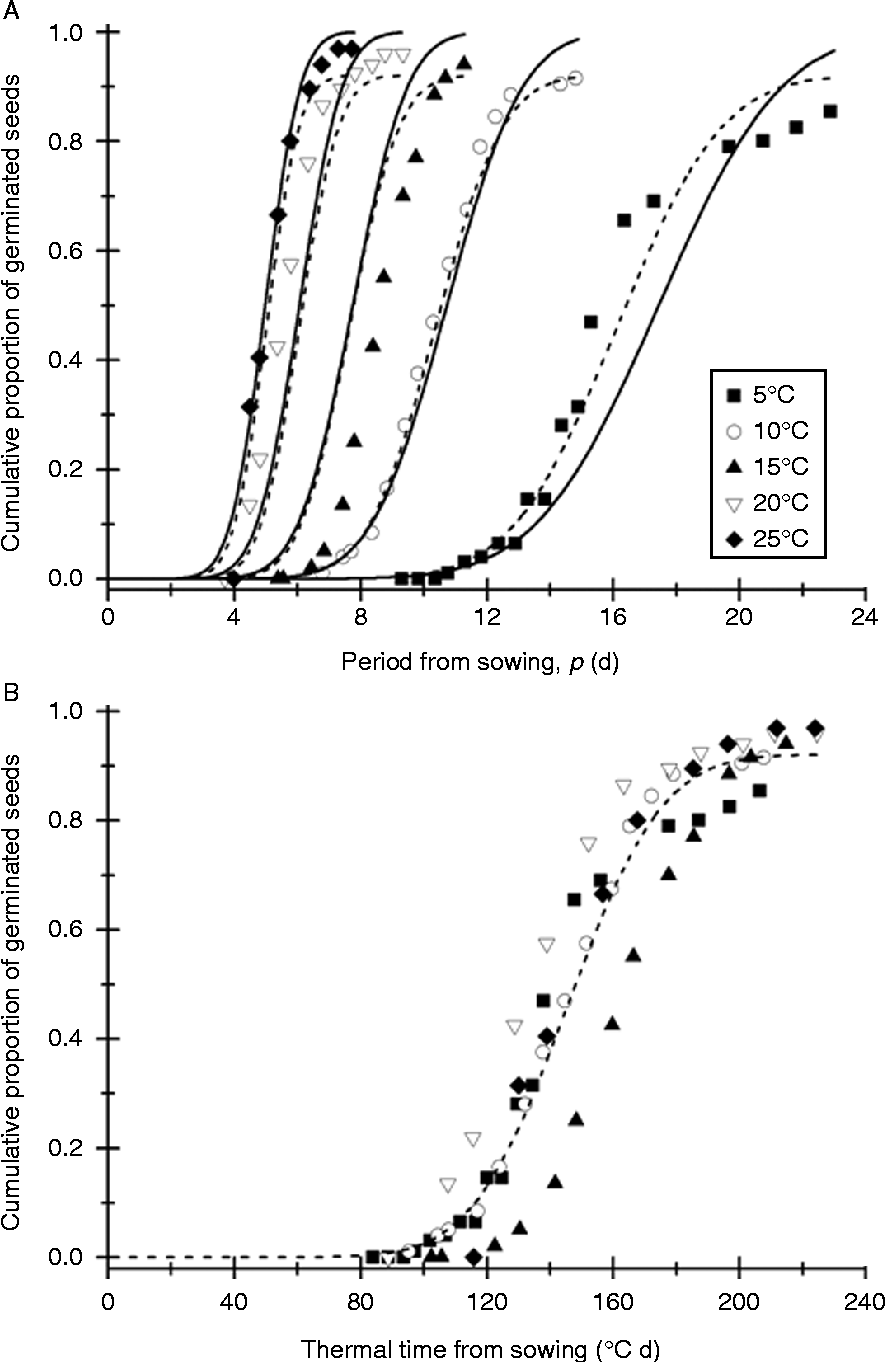
In this model, the parameters to be determined are β₀, the initial germination in probits and β₁ which describes the rate of increase in probit germination as the explanatory variable, in this case, thermal time (above T _b) increases. The reciprocal of β₁ is the standard deviation of the distribution of thermal times to germination. This parameter is known as the thermal time constant, θ_T. In this GLM, T _b is also unknown but can be estimated within the probit analysis. This may not be possible through standard software GLM menus (which require the specification of explanatory variable values); however, it may be possible using statistical software programming languages. For example, in GenStat, as with fitting the combined viability equation (equation 12), this is possible using the FITNONLINEAR directive, as demonstrated (Fig. 3) for germination data for seeds of faba bean (Vicia faba L.) cv. Sutton taken from Ellis et al. (Reference Ellis, Simon and Covell1987). In that paper, the mean T _b (for g= 10, 20, 30, 40, 50, 60, 70, 80 and 90% germination) was estimated (by going up in steps of 0.5°C) as − 3.0°C; the estimate using GenStat to fit equation (15) was − 3.70°C (SE 0.372). Further, there was a significant (P< 0.001) reduction in the residual deviance when a ‘C _v’ (control viability) parameter was also included in the GLM to estimate the maximum level of viability:

Figure 3

Thermal time probit analysis modelling of faba bean germination data taken from figure 1 in Ellis et al. (Reference Ellis, Simon and Covell1987). (A) Approximate raw data for the progress of seed germination over time at the temperatures indicated, showing the fitted germination progress curves using the published thermal time model parameters (solid lines) and the results of using the FITNONLINEAR directive in GenStat to fit the GLM with the inclusion of the C _v parameter (equation 16) (dashed lines). There were significant decreases in the residual deviance when parameters were estimated in the GLM rather than set at the published values (F _3,65= 22.7, P< 0.001) and when the C _v parameter was then included (F _1,64= 13.26, P< 0.001). Parameter estimates: β₀= − 6.13 (SE 0.462), β₁= 0.042 (SE 0.0034), T _b = − 4.03 (SE 0.367) and C _v = 0.921 (SE 0.0204). (B) The same data plotted against thermal time calculated using the fitted model (with C _v).

This equation is perhaps easier to comprehend in toto than equation (14), in which the percentage germination, g, can take any value (0–100). Fitting equation (16) to the data as a GLM is done in a single step; there is no interpolation of germination progress curves to determine the time for germination to reach, for example, 10, 20, 30,…%. Further, this approach does not rely on ‘manual’ setting and adjustment of T _b values and assessment of the residual sum of squares. Most importantly, this method of analysis takes into account all the raw data and the inherent variability (error distribution) in that data.

Hydrotime

Following on from the concept of thermal time above a base temperature, T _b, for germination, described by Garcia-Huidobro et al. (Reference Garcia-Huidobro, Monteith and Squire1982), Gummerson (Reference Gummerson1986) proposed a model describing the effect of water potential on germination. In this ‘hydrotime’ model, the base water potential, ψ_b, was assumed to vary between individual seeds within the population, again following a normal distribution. Gummerson (Reference Gummerson1986) and others have usually defined the hydrotime model, at a single constant temperature, using the equation:

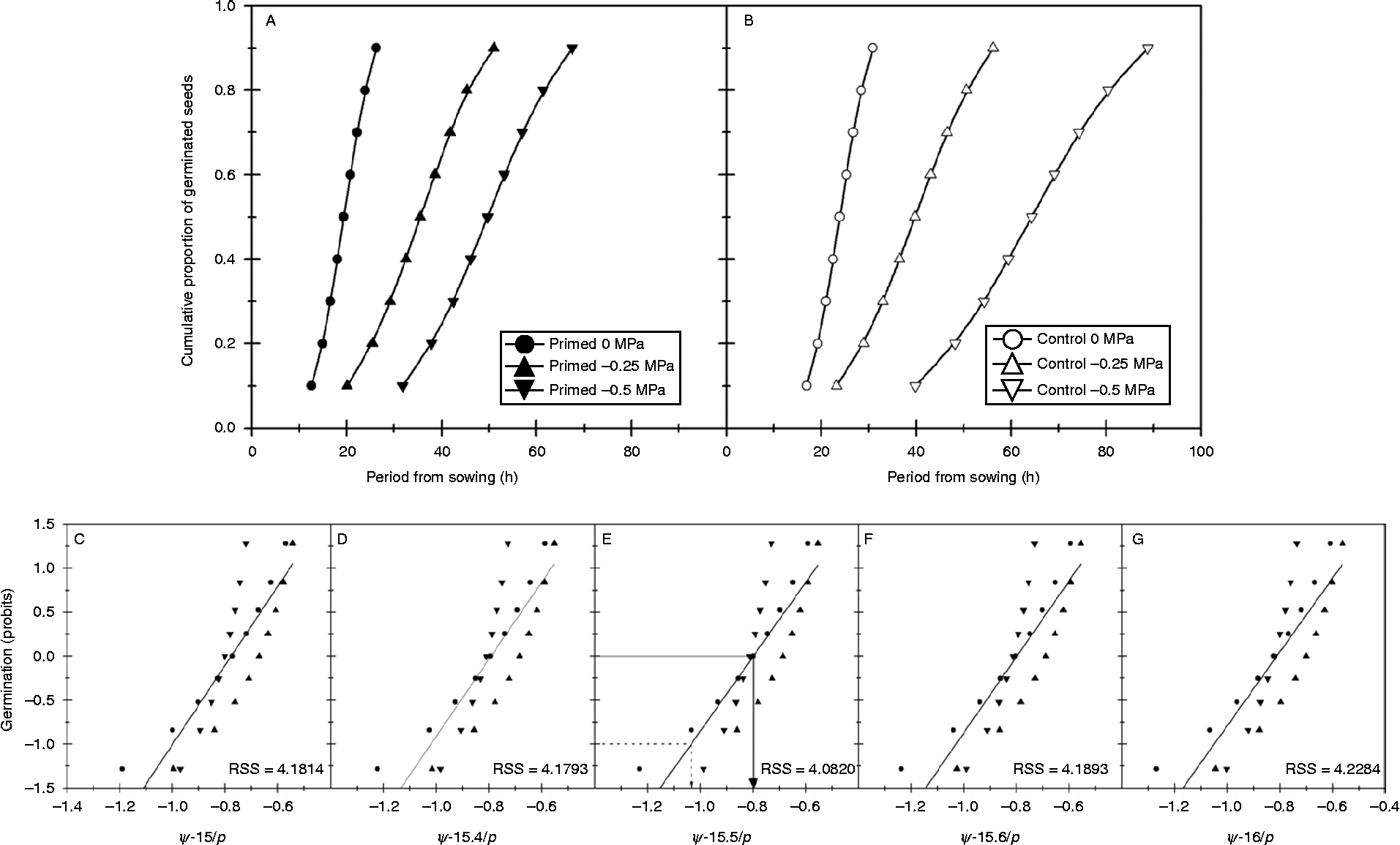
where GR _g is the ‘germination rate’ as before; ψ is water potential and ψ_b(g) is the minimum water potential for % germination, g; and θ_H is the ‘hydrotime constant’, assumed to be the same for all seeds (Bradford, Reference Bradford1990, Reference Bradford2002; Bradford and Still, Reference Bradford and Still2004; Golaszewski and Bochenek, Reference Gołaszewska and Bochenek2008). Since the model assumes that the variation in ψ_b between individual seeds within the population follows a normal distribution, there is a linear relationship between probit germination and ψ_b. A further implication of this equation is that seeds with a value of ψ_b that is less negative than ψ will have a germination rate that is negative, and therefore germination will not occur. This is in contrast to the thermal time model described above, in which T _b is assumed constant for all seeds within the population and where, therefore, it is expected that all seeds will eventually germinate once they have spent enough time at temperatures above T _b (Bradford, Reference Bradford, Kigel and Galili1995). The procedure that has been adopted for determining ψ_b is an adaptation of the method Ellis et al. (Reference Ellis, Simon and Covell1987) used to determine T _b; linear regression analysis is carried out for probit germination against (ψ–θ_H p ^− 1) with the value of θ_H adjusted until the residual sum of squares (RSS) is minimized (Fig. 4C–G). Since it uses probit germination as the dependent variable, this method has been termed ‘repeated probit analyses’ (e.g. Dahal and Bradford, Reference Dahal and Bradford1990). The median base water potential for germination, ψ_b(50) is where probit germination = 0 and the standard deviation of the distribution of ψ_b, σ_ψb, is the inverse of the slope of the linear relationship. For the data for primed lettuce seeds shown in Fig. 4 (from Bradford and Still, Reference Bradford and Still2004), using this method of model fitting, θ_H= 15.5, ψ_b(50) = − 0.8 MPa and σ_ψb= 0.23.

Figure 4

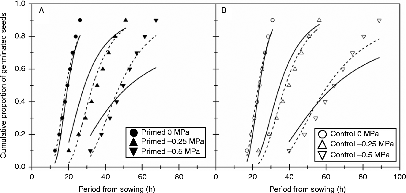
Hydrotime modelling of data given for primed and non-primed (‘control’) seeds of lettuce in Bradford and Still (Reference Bradford and Still2004). The data presented in that publication, plotted in (A) and (B), give the times for germination to reach 10, 20,…, 80 and 90%, rather than raw data following the progress of seed germination (i.e. involves interpolation of germination progress curves). The recommended procedure for hydrotime model fitting involves repeated probit analyses (Ellis et al., Reference Ellis, Simon and Covell1987) whereby linear regression analysis is carried out of probit germination against (ψ – θ_H p ^− 1) with the value of θ_H adjusted until the residual sum of squares (RSS) is minimized ((C)–(G) primed seeds only, regression analysis carried out using Origin 8.1). For these data, the RSS is least when θ_H= 15.5 (to 1 dp; E), ψ_b(50) = − 0.8 MPa (solid line arrow) and σ_ψb= 0.23 (the inverse of the slope or, as shown by the difference between the dashed and solid line arrows, the change in ψ for germination to increase by 1 probit).

The hydrotime model may also be expressed as a GLM (Golaszewski and Bochenek, Reference Gołaszewska and Bochenek2008) and the hydrotime parameters estimated more simply using probit analysis directly. The GLM for the hydrotime model has the form:

Expressing the hydrotime model in this form identifies an implicit assumption that, at constant water potential, it is the reciprocal of time to germination (p ^− 1) that is normally distributed, rather than time to germination (p). This is consistent with one of the approaches suggested above for modelling germination as a function of time where the cumulative germination curves are asymmetric (Fig. 2B–C).

To fit the hydrotime model as a GLM (equation 18), the data are entered as before, as the number of seeds that germinated and the number of seeds sown for the dependent variable, g, and with two explanatory variables, ψ and p ^− 1. The probit analysis will provide estimates for the three unknown parameters in the GLM from which it is possible to calculate the familiar hydrotime parameters: θ_H= − β₂/β₁, ψ_b(50) = − β₀/β₁ and σ_ψb= 1/β₁. This was done for the Bradford and Still (Reference Bradford and Still2004) lettuce seed data, using the ‘Modelling of binomial proportions’ routine in the GLM menu of GenStat 13 and assuming 100 seeds were sown at each water potential. For primed seeds the fitted model gave estimates for β₀, β₁ and β₂ of 3.49 (SE 0.163), 4.39 (SE 0.230) and − 68.7 (SE 3.19), respectively; it follows that θ_H= 15.65; ψ_b(50) = − 0.79 and σ_ψb= 0.23 (Table 1 and Fig. 5). The discrepancy in parameter values, most notably for θ_H, reflects the different weights associated with observations in the different analysis approaches.

Table 1

Results of probit analysis to fit the hydrotime model (equation 18) to the Bradford and Still (Reference Bradford and Still2004) lettuce seed data shown in Fig. 4A, B. Probit analysis was carried out using the ‘Modelling of binomial proportions’ routine in GenStat 13 with a probit link function. For the independent model, the ‘Model to be fitted’ took the form seed-lot*(ψ + p ⁻¹); for the constrained model, the seed-lot factor was not included in the model fitting

* The fit of the models was compared using an approximate F-test; there was a significant increase in residual deviance when the constrained model was fitted compared with the independent model (P< 0.001). However, the best model is clearly one in which an interaction term^† is included (and hence θ_H is allowed to vary). x indicates that the term was not included (β₃) or that it is not possible to calculate the derived parameters.

Figure 5

Using probit analysis to directly fit the hydrotime model to the lettuce seed germination data from Bradford and Still (Reference Bradford and Still2004) shown in Fig. 4A, B. The solid fitted lines show the results of independent fitting of the model for primed and control seeds (equation 18; Table 1). Fits were improved by including an interaction term, i.e. allowing θ _H to vary (equation 19; dashed lines).

By including seed-lot treatments as factors in the analysis, it is also possible to determine whether β₀, β₁ and β₂ differ significantly between those seed-lot treatments by analysis of the residual deviance (in the situation where the data are assumed to be independent). For example, for the lettuce seed data, there was a significant increase in the residual deviance when all three model parameters (β₀, β₁ and β₂) were not allowed to vary between primed and control seeds (P< 0.001; Table 1, Fig. 5). Fitting the hydrotime model to the lettuce data with seed-lot treatment as a factor showed that priming increased the rate of germination (decreased θ_H ( = − β₂/β₁)) and increased the variation between individual seeds in their response to water stress, although there was no change in ψ_b(50) ( = − β₀/β₁). As well as priming, other treatments may alter the hydrotime model parameters; for example, Zuk-Gołaszewska et al. (Reference Zuk-Gołaszewska, Bochenek and Gołaszewski2007) concluded that breaking physical dormancy through scarification significantly decreased θ_H for seeds of red clover, while ψ_b(50) and σ_ψb were relatively unchanged. However, since θ_H is dependent on two of the GLM parameters, β₁ and β₂, and ψ_b(50) and σ_ψb also vary if there is change in β_1, this is not easy to test specifically through a process of allowing individual parameters to vary with treatment (e.g. priming or scarification) in the GLM. The parameter β₀ is an estimate of the maximum germination that could be achieved by the seed-lot. This is not usually estimated when fitting is done by linear regression analysis of probit germination against (ψ – θ_H p ^− 1) for different values of θ_H. Estimates of β₀>3.00 (Table 1) are equivalent to maximum germination greater than 99.87%.

Using probit analysis to fit the GLM described by equation (16) assumes that θ_H is constant for all seeds in the population; this is generally accepted to be the case (Gummerson, Reference Gummerson1986; Bradford, Reference Bradford1990, Reference Bradford, Kigel and Galili1995, Reference Bradford2002; Kebreab and Murdoch, Reference Kebreab and Murdoch1999b). However, the validity of this assumption could be considered by comparing the fit of this standard model (equation 18) with that including an additional interaction term:

Including this interaction term, as well as the seed-lot factor, to analyse the lettuce data (i.e. fitting equation 19 to the primed and control data simultaneously) resulted in further reductions in the residual deviance (Table 1, Fig. 5). Formal model testing would allow the assessment of whether this more complex model provides a better fit to the data, but the implication that θ_H varies within the seed-lots needs careful thought about the mechanistic interpretation of this more complex model. Implementation of the hydrotime model as a GLM thus allows the exploration of a wider range of potential models to describe the observed data, although care is needed in the derivation of the traditional hydrotime model parameters and in the interpretation of the underlying biology for any more complex models so derived.

Hydrothermal time

Gummerson (Reference Gummerson1986) also considered the combined effect of temperature and water potential on the rate of germination of sugar beet seeds, using the thermal time theory of Garcia-Huidobro et al. (Reference Garcia-Huidobro, Monteith and Squire1982) as a starting point (equation 14). Mirroring the form of this thermal time equation, but with water potential replacing temperature, and using thermal time rather than time, Gummerson (Reference Gummerson1986) defined:

where θ_HT is the ‘hydrothermal time’ constant, the accumulated period of time spent at water potentials above the base water potential and temperatures above the base temperature required for germination of the gth percentile of the population. Combining equation (14) and equation (20), the hydrothermal time constant can then be expressed as:

where T and ψ are temperature and water potential, respectively; T _b is the base temperature for g% germination, ψ_b is the base water potential and p _g is the period of time from sowing for g% germination (Gummerson, Reference Gummerson1986; Dahal et al., Reference Dahal, Bradford, Haigh, Côme and Corbineau1993; Dahal and Bradford, Reference Dahal and Bradford1994). In equation (21), θ_HT and T _b are assumed to be constant for all seeds within a seed-lot, while ψ_b is allowed to vary. Gummerson (Reference Gummerson1986) stated that ‘… a normal distribution is the most likely description…’ of the distribution of base water potentials within a seed-lot.

This derivation of hydrothermal time identifies key differences in the underlying assumptions for the thermal time and hydrotime models. In the thermal time model, it is the thermal time to germination that is allowed to vary with the base temperature fixed, while in the hydrotime model the hydrotime to germination is fixed with the base water potential allowed to vary. A comparison of the GLM parameterizations of the thermal time (equation 15) and hydrotime (equation 18) models highlights this difference in how time is included: in the first case probit germination changes linearly with time and in the second linearly with the reciprocal of time. Similarly, equation (20), expressing 1/θ _T as a function of water potential, is different to the equivalent equation for hydrotime (equation 17), in which 1/p _g is expressed as a function of water potential. Finally, combining equations (14) and (20) with the assumption that base water potential follows a normal distribution within a seed-lot, means that the assumption made by some (e.g. Ellis et al., Reference Ellis, Covell, Roberts and Summerfield1986, Reference Ellis, Simon and Covell1987) that thermal time to germination follows a normal distribution, cannot be true. In fact, the implication is that the reciprocal of thermal time to germination follows a normal distribution, supporting observations (e.g. Campbell and Sorenson, Reference Campbell and Sorensen1979; Scott and Jones, Reference Scott and Jones1985; Dahal et al., Reference Dahal, Bradford and Jones1990) that thermal time to germination often follows a skewed (e.g. log-normal, inverse normal) rather than a symmetric (e.g. normal) distribution at a constant water potential.

The hydrothermal time model has been applied widely and, again, the repeated probit analyses method has been the preferred approach to first fit the thermal time and hydrotime models separately, and then the combined hydrothermal time model to estimate the hydrothermal time parameters, θ_HT, T _b, ψ_b(50) and σ_ψb (e.g. Dahal and Bradford, Reference Dahal and Bradford1994; Alvarado and Bradford, Reference Alvarado and Bradford2005; Graziani and Steinmaus, Reference Graziani and Steinmaus2009; Zambrano-Navea et al., Reference Zambrano-Navea, Bastida and Gonzalez-Andujar2013). Rowse and Finch-Savage (Reference Rowse and Finch-Savage2003) used the same, repeated probit analyses method to fit an extended hydrothermal time model that incorporates modifications to the base water potential distribution at supra-optimal temperatures to model the reduction in germination rate observed at these temperatures.

As with the earlier models, the hydrothermal time model may also be fitted as a GLM:

and the hydrothermal time constant, θ_HT, calculated as − β₂/β₁. This parameterization emphasizes that it is the reciprocal of thermal time, (p(T – T _b))^− 1, that is assumed to be normally distributed, and not thermal time. Again, the parameter β₀ is an estimate of the maximum germination which would not otherwise be estimated. Since T _b is unknown, as for the thermal time model, this GLM would have to be fitted through non-linear model fitting. Bloomberg et al. (Reference Bloomberg, Sedcole, Mason and Buchan2009) fitted a hydrothermal time model to germination data for Pinus radiata (D. Don) at sub-optimal temperatures using the ‘nls’ function in the statistical software R, but transformed the percentage germination to probit germination values (i.e. fitted a LM to probit values) rather than fitting a GLM directly. Re-analysing the P. radiata data using the FITNONLINEAR directive in GenStat 13, there were significant improvements (reduction in overall residual deviance) when the model is fitted as a GLM compared with the stepped approach, as determined by setting the values of β₀, β₁ and β₂ as − ψ_b(50)/σ_ψb, 1/σ_ψb and − θ_HT/σ_ψb, respectively, using the values published in Bloomberg et al. (Reference Bloomberg, Sedcole, Mason and Buchan2009) (Table 2). Further improvements were gained by adding a C _v (control viability) parameter to the model to estimate the maximum level of germination, as can be seen from the reduction in overall residual deviance (Table 2) and the fitted curves that, for many combinations of temperature and water potential, are closer to the observed data (Fig. 6).

Table 2

Results of probit analysis to fit the hydrothermaltime model to data for Pinus radiata from Bloomberg et al. (Reference Bloomberg, Sedcole, Mason and Buchan2009). Probit analysis was carried out using the FITNONLINEAR directive in GenStat 13. The first model (‘Bloomberg Model 1’) used the estimates for $$\theta _{HT} $$ , $$\psi _{b}\left (50\right ) $$ and $$\sigma _{ \psi _{b}} $$ to determine the value of the parameters β₀, β₁ and β₂ in the model (these were not allowed to change). There was a significant reduction in the residual deviance when these parameters were allowed to change (P<0.001) and when an interaction term was subsequently included in the model (P<0.01). For each of these three models, there was a further reduction in residual deviance when the control viability (C _v) parameter was included in the model fitting

^A–EResults of model fitting shown in Fig. 6A–E; ^F–J results of model fitting shown in Fig. 6F–J. x indicates that the term was not included (β₃) or that it is not possible to calculate the derived parameters.

Figure 6

Results of GLM fitting of the hydrothermal time model to data for Pinus radiata from Bloomberg et al. (Reference Bloomberg, Sedcole, Mason and Buchan2009) at the water potentials (MPa) shown in the boxes in (A) and (F). Probit analysis was carried out using the FITNONLINEAR directive in GenStat 13 with model parameters either (A–E), set to those determined by Bloomberg et al. (Reference Bloomberg, Sedcole, Mason and Buchan2009; model 1) or (F–J) allowed to vary while also estimating the control viability parameter (Table 2). The standardized residuals shown in (E) and (J) are those generated by GenStat for each corresponding model.

Bloomberg et al. (Reference Bloomberg, Sedcole, Mason and Buchan2009) and Watt et al. (Reference Watt, Xu and Bloomberg2010) emphasized the importance of model criticism and improvement to enhance our understanding of the underlying physiological processes in seeds. Another advantage of fitting the hydrothermal time model as a GLM is that standardized residuals can be automatically generated. The plot of these standardized residuals from the GLM fitted using the P. radiata parameters (model 1) determined by Bloomberg et al. (Reference Bloomberg, Sedcole, Mason and Buchan2009) also shows evidence of curvature (Fig. 6E). This curvature in the residual plot was much less apparent when the hydrothermal time model was fitted as a GLM with parameters allowed to vary (Fig. 6J), although when the residuals are plotted for each treatment combination (temperature ×  water potential), there is still evidence of systematic deviation between observed and fitted values which varies between treatments (as can also be seen in Fig. 6F–I). Curvature in residual plots may result from changes in seed germinability during the germination time course, with a consequent change in hydrothermal time model parameters. Bloomberg et al. (Reference Bloomberg, Sedcole, Mason and Buchan2009) modified the model for P. radiata to take into account an upward shift in ψ_b with increasing time to germination. Similarly, Kebreab and Murdoch (Reference Kebreab and Murdoch1999b) found that there were interactions between temperature and ψ such that ψ_b(50) varied depending on temperature and T _b varied depending on ψ.

Other ‘threshold models’

The thermal time, hydrotime and hydrothermal time models are examples of what have been termed ‘threshold models’, described by Bradford (Reference Bradford2005) as being ‘… based on the concept that the magnitude or speed of a biological response is proportional to the difference between the level of a signal input and the threshold sensitivity for that input’. For these models this description is perhaps too simplistic as there are two threshold components: the base level of the input (i.e. base temperature or base water potential) above which germination processes within a seed can commence, and the amount of accumulated time (e.g. thermal-, hydro- or hydrothermal time) above these base levels required for germination of that seed to be completed. Thus, if the signal input for a seed is below the base level, the germination process will not commence; if the base level varies within a population, such as is assumed in the hydrotime model, then the proportion of seeds within a seed-lot that will germinate will also vary. Further, as the signal level increases above the base level, the progress towards germination is accelerated. It is worth reiterating that in the thermal time model it is the accumulated thermal time (above a fixed threshold, T _b) required to complete germination that varies within a seed-lot, while in the hydrotime model the accumulated hydrotime required for germination is fixed, but the base water potential varies within the population, as a function of germination percentile (g).

Threshold models have also been used to describe the effects of other variables that either slow the rate of germination and/or reduce the final proportion of seeds that germinate or accelerate the rate of germination and/or increase the proportion of seeds that germinate, where the thresholds (base level and/or accumulated time) are assumed to follow a normal distribution. For example, instead of water stress, Bradford et al. (Reference Bradford, Tarquis and Duran1993) considered the effect of experimental storage on the progress of seed germination for lettuce seeds, thereby combining the normal distribution of seed deaths over time as incorporated in the seed viability equation (Ellis and Roberts, Reference Ellis and Roberts1980a) with the normal distribution of seed germination over p ^− 1. The GLM for this model would therefore take the form

where p _ES refers to the period of time in experimental storage and p _GT refers to the period of time in the germination test. Here p _ES is the signal input to the threshold model with each seed having a base storage period (assumed to follow a normal distribution) after which they no longer have the ability to germinate. Where p _ES is less than the base storage period for a seed, the time to germination, p _GT, will decrease as the difference between the signal input, p _ES, and the base storage period increases. Hence, both β₁ and β₂ should have negative estimates, so that the relationships between the GLM parameters and the conventional threshold model parameters (as identified above for the hydrotime model) indicate that θ_age (the ageing time constant) should take negative values (also inferred by equation 4 in Bradford et al., Reference Bradford, Tarquis and Duran1993).

Using probit analysis in statistical software, the germination response to alternative/multiple explanatory variables, where the response to each variable is expected to follow a normal distribution (either with or without transformation), can be as easily evaluated as a simple or multiple linear regression model; for example, to model the germination response to three explanatory variables [p ^− 1, ψ (as for the hydrotime model) and log(abscisic acid concentration)], as described by Ni and Bradford (Reference Ni and Bradford1992). Explanatory variables with a potentially positive effect on the germination of dormant seeds, which could likewise be incorporated into the probit GLM, include, as continuous variables, (log) gibberellic acid concentration (Ni and Bradford, Reference Ni and Bradford1993), after-ripening period (Gianinetti and Cohn, Reference Gianinetti and Cohn2007; Chantre et al., Reference Chantre, Batlla, Sabbatini and Orioli2009) and after-ripening thermal time (Bazin et al., Reference Bazin, Batlla, Dussert, El-Maarouf-Bouteau and Bailly2011), or as qualitative treatments, exposure to heat or smoke relative to an untreated control (Thomas et al., Reference Thomas, Morris, Auld and Haigh2010). Kebreab and Murdoch (Reference Kebreab and Murdoch1999a) considered the effects of loss of primary dormancy, induction of secondary dormancy and loss of viability for seeds of Orabanche aegyptiaca Pers., O. cernua Loefl. and O. crenata Forsk., but this model is not a typical threshold model as it does not include the accumulated period of time required to achieve different levels of germination. In constructing models with more explanatory variables, it may be necessary to consider interacting effects where such interactions have a justifiable biological interpretation. It should also be noted that more data are of course required in order to fit the increased number of parameters required by these models. Experiments designed with a complete factorial treatment structure will ensure that these interaction effects can be fully estimated.

Survival analysis methods and analysing the distributions of times to response

As identified above, it is generally not appropriate to analyse the cumulative germination curve data collected in germination studies using probit analysis (within the GLM framework) because the observed germination counts at successive time-points are not independent. While alternative analysis methods, including the concept of survival analysis and the fitting of statistical distribution functions to observations of times to germination, have been explored (e.g. Scott et al., Reference Scott, Jones and Williams1984), these methods have not been applied widely or routinely in seed germination studies (McNair et al., Reference McNair, Sunkara and Frobish2012; Manso et al., Reference Manso, Fortin, Calama and Pardos2013; Ritz et al., Reference Ritz, Pipper and Streibig2013). This may be, in part, due to the nomenclature used to describe these models: germination studies are concerned with the time to evidence of life, not with the time to death (or failure), so the idea of using survival analysis may not seem compatible. Further, studies tend to be focused on recording the number of seeds that have germinated (by a particular time), rather than on the actual times of germination for individual seeds. This again suggests that these methods would not be appropriate, since they appear to be concerned with analysis of data in the form of times. Conversely, survival analysis methods are not appropriate for analysing data from seed survival studies as it is never known when each individual seed dies (Hay et al., Reference Hay, Smith, Ellis and Butler2010) and assessment of viability after periods of storage can only be made through destructive testing (i.e. a germination test) of independent samples of multiple seeds.

More recently, there have been several publications concerned with the application of survival analysis approaches to seed germination data, as reviewed by McNair et al. (Reference McNair, Sunkara and Frobish2012). Onofri et al. (Reference Onofri, Gresta and Tei2010) considered a range of Accelerated Failure Time (AFT) models (similar to the accelerated life models described briefly earlier) to describe germination responses for four different weed species, based on the initial calculation of a non-parametric Kaplan–Meier estimator of the probability of germination at any point in time. This is calculated as a function of the number of seeds that have germinated in each time interval prior to that point in time, and the number of seeds that were available to germinate at the end of the preceding interval (Cox and Oakes, Reference Cox and Oakes1984). The AFT approach allows consideration of a range of statistical distribution functions for the times to germination of seeds in a seed-lot, including the exponential, Weibull, log-normal and log-logistic, and allows comparison of the responses for different seed-lots through estimation of an ‘acceleration factor’ that summarizes the relative germination rates of the seed-lots, but assumes a common shape of response (i.e. a common form of statistical distribution). Other survival analysis approaches include the semi-parametric Cox proportional hazards model and the non-parametric actuarial life table method (Cox and Oakes, Reference Cox and Oakes1984). While these methods can provide a good description of observed germination responses, how well they can be used in a predictive capacity for data sets collected across a wide range of environmental conditions, as in the threshold models described above, is not clear. However, Manso et al. (Reference Manso, Fortin, Calama and Pardos2013) demonstrated one approach where the hazard function is modelled as the product of non-linear functions of a set of potential explanatory variables, although it is not immediately clear how this then relates to the existing thermal, hydro- and hydrothermal-time models. As already identified, another issue for the application of survival analysis models to seed germination data is that conventional survival analyses will include censored observations for individuals who have survived to the end of the study period. With seed germination studies, as mentioned previously, it is often unknown whether seeds that have not germinated at the end of the study are still viable, and so it is difficult to know how to include these seeds in the data analysis.

The alternative approach to analysing time to response data is to model the distribution of times directly, based on the numbers of seeds germinating in a series of observation intervals. An initial development of such an approach was described by Hunter et al. (Reference Hunter, Glasbey and Naylor1984) based on the assumption that the times to germination followed a normal distribution, possibly after some transformation of the time variable, and including a further parameter to estimate the proportion of the seed-lot that was viable (with the further assumption that the non-viable seeds were not part of the normal distribution of times to germination). A similar approach was applied by O'Neill et al. (Reference O'Neill, Thomson, Jacobs, Brain, Butler, Turner and Mitakda2004) with a focus on using the inverse normal distribution to describe times to germination for perennial ryegrass. In both cases the approach uses a maximum likelihood method to fit the chosen distribution function to the observed germination counts in each interval, essentially by predicting the cumulative germination count at the start and end of each interval and thus obtaining the predicted count for that interval.

Hence, the hydrothermal time model could be implemented with the common assumption that the base water potentials within a seed-lot follow a normal distribution, that germination progress is a function of accumulated hydrothermal time above the base water potential and base temperature, and, as a consequence of the assumption regarding the distribution of base water potentials within a seed-lot, that germination events in thermal time follow an inverse normal distribution. Here the data would be arranged as the number of seeds germinating in each time interval for each of a number of combinations of constant temperatures and water potentials. The maximum likelihood estimation process starts with initial estimates of all of the model parameters and then uses an iterative optimization process to search the parameter space for the combination of parameters that produces predictions that most closely match the observed responses in each time interval for each combination of treatments. An implementation of this approach (available from the second author), for the modified version of the hydrothermal time model proposed by Rowse and Finch-Savage (Reference Rowse and Finch-Savage2003), using the generalized regression facilities in GenStat (VSN International), includes expressions to calculate the base water potentials for the percentile of the seed-lot to have germinated at the start and end of each time interval, based on the assumption that these values follow a normal distribution, to estimate the overall proportion viability of the seed-lot (assumed to be constant across all treatment combinations) and to calculate the (constant) base temperature and hydrothermal time constant, and hence predict the number of seeds that should germinate in each time interval.

The major benefit of this approach is in the flexibility it allows in the choice of models to describe observed germination responses. Mesgaran et al. (Reference Mesgaran, Mashhadi, Alizadeh, Hunt, Young and Cousens2013) consider a range of statistical distribution functions to describe the distribution of base water potentials within a seed-lot, and the consequent cumulative distribution functions for percentage germination as a function of time and water potential. The proposed models include a number of the distributions identified earlier as being considered as possible models for the distribution of failure times within the survival analysis approach – the Weibull distribution, log-normal distribution, log-logistic distribution and gamma distribution – as well as the inverse normal distribution. While they acknowledge the need to use a maximum likelihood approach to fit these models to their observed data, and the lack of independence between germination counts at consecutive observation times, their results appear still to be based on fitting the cumulative distribution functions to the observed cumulative germination data, despite an acknowledgement and demonstration (in their online supplementary material) of the bias in the parameter estimates and underestimation of the standard errors associated with these biased parameter estimates. An earlier study (Watt et al., Reference Watt, Xu and Bloomberg2010) compared the use of normal and Weibull models for the distributions of base water potentials within a seed-lot in fitting the hydrothermal time model to germination data for two species [P. radiata and Buddleja davidii (Franch.)]. Again, however, despite using a non-linear regression approach, they fit cumulative distribution functions to the cumulative germination counts and so are likely to be introducing the same bias and underestimation of errors as are identified above.

Watt et al. (Reference Watt, Xu and Bloomberg2010, Reference Watt, Bloomberg and Finch-Savage2011) and Mesgaran et al. (Reference Mesgaran, Mashhadi, Alizadeh, Hunt, Young and Cousens2013) suggest that some alternative to the assumption that base water potentials follow a normal distribution provides a better fit to the observed (cumulative) germination data, suggesting either the Weibull or the log-logistic distribution. Both distributions have skewed probability density functions, which are not too dissimilar in shape to the probability density function for the inverse normal distribution. Therefore the adoption of these alternative forms of distribution for the base water potentials within a seed-lot in a hydrothermal time model might overcome the contradiction caused by the assumptions made by Gummerson (Reference Gummerson1986) and others in the original development of the hydrothermal time model, about the distributions of the thermal time to germination and base water potentials.

A commonly stated barrier (e.g. Mesgaran et al., Reference Mesgaran, Mashhadi, Alizadeh, Hunt, Young and Cousens2013) to the fitting of models to non-cumulative germination counts rather than cumulative germination counts is the inaccessibility of approaches to fit such models within modern computer packages. Yet such an approach was implemented by Hunter et al. (Reference Hunter, Glasbey and Naylor1984) nearly 30 years ago and O'Neill et al. (Reference O'Neill, Thomson, Jacobs, Brain, Butler, Turner and Mitakda2004) described the implementation of such an approach within the commercially available statistical computing package GenStat nearly 10 years ago, based on the development of the GenStat function CUMDIST by Brain and Butler (Reference Brain and Butler1988). Recent papers (e.g. Watt et al., Reference Watt, Xu and Bloomberg2010, Reference Watt, Bloomberg and Finch-Savage2011; Mesgaran et al., Reference Mesgaran, Mashhadi, Alizadeh, Hunt, Young and Cousens2013) describe the use of standard non-linear regression modelling routines to fit these cumulative models, usually requiring the specification of the form of the model using a number of expressions. The extension of this approach to define a model for the difference between two cumulative counts (i.e. at the start and end of each observed time period) should be straightforward using such non-linear regression modelling routines, as described above for the Rowse and Finch-Savage (Reference Rowse and Finch-Savage2003) model.

Having adopted this more general modelling approach to the analysis of germination progress curves, the development of more complex models should be possible, to incorporate an even wider range of stimuli. This more general approach allows access to a much wider range of model forms for the distribution of base water potentials within the existing hydrothermal time model framework. This modelling approach could also allow the redevelopment of a hydrothermal time model in which the impacts of temperature and water potential are not so closely linked, possibly also allowing the formal inclusion of some form of interaction between the effects of temperature and water potential, should that be appropriate. Of course, these further developments should be firmly grounded in a biological (mechanistic) understanding of the processes involved, rather than just based on the best fitting model from a statistical perspective, but this more general modelling approach does then allow the comparison of models with a range of different assumptions and structures.