Grappling with Prediction: Progress in Meteorology from 1914 – 1945

Meteorology is for many reasons a fruitful field to interrogate if one is interested in epistemological questions about modeling. Over the course of its emergence as a discipline it presents a confluence of multiple traditions that had to contend with how best to communicate and cohabitate (Galison Reference Galison1997, chap. 9). It presents a marked historical shift from strict mathematization to patchwork modeling. And finally, many crucially important tensions – statistics versus dynamics, prediction versus understanding, and so on – played out in a most acute fashion (Dahan Dalmedico Reference Dahan Dalmedico2001, 396). Meteorology can also offer a certain generality in some of the insights it generates: the role of models based on fluid dynamics in meteorology tie in with hydrology, glaciology, oceanography, aeronautics, astronomy, and more besides (Nebeker Reference Nebeker1995, 185; also Star and Griesemer Reference Star and Griesemer1989). Alongside this general epistemological promise, however, lies a very particular history. Having received a boost in the nineteenth century from fields ranging from agriculture to commerce to public health, meteorology was propelled by war into even greater prominence over the first half of the twentieth century. In 1919, physicist Robert Millikan claimed World War I to be the first major conflict in which a meteorological section proved indispensable (Millikan Reference Millikan1919; see also Nebeker Reference Nebeker1995, 84).Footnote ⁸ Important developments also came during the interwar period, with the profession continuing to grow as fresh forecast demands came from land, sea, and air travel concerns, the insurance industry, and agencies of government concerned with wildfire control and the alleviation of drought.Footnote ⁹ Yet it was undeniably World War II that fueled the most vigorous and important expansion in the first half of the century. For the effective timing of operations such as Overlord, accurate forecasts played a quite crucial strategic and logistical role. Additionally, certain contingencies of war – most obviously a compressed timeframe in which to train the new cohorts of forecasters – had a tangible impact on pedagogical practice that would persist well beyond the end of conflict in 1945. Concretely speaking, and even in the absence of any one “master algorithm” that could demonstrably and consistently outperform “subjective” forecasters, the need for quick apprehension made more algorithmic approaches very appealing indeed. World War II also pressured meteorologists to increase both the detail and the range of their forecasts. With respect to detail there was a clear improvement; with respect to temporal range the results were rather mixed. As Nebeker has shown, until 1940 the weather services of both the United Kingdom and the United States did not venture a forecast beyond two or three days. Under pressure from the military, this was rolled out to five days, but while these longer-range forecasts were reliable enough for the first day they were rather less so thereafter. One analysis compared the results from actual five-day forecasts to a pseudo-forecast in which it was simply stipulated that the final four days would always resemble the first. The results of this pseudo-forecast were no worse than the actual one (Stagg Reference Stagg1971, 32).Footnote ¹⁰ Yet despite these almost embarrassing difficulties in deriving sharper forecasts beyond a certain range – here hardly any progress had been made since the turn of the century – the immediate postwar period in meteorology was very much buoyed by the war. Militarization had brought an increase in trained personnel, a greater stock of experience, greater financial resources, an improved data network, and several novel pedagogical approaches.Footnote ¹¹ This in turn served to create conditions of possibility for new institutional formations, the most useful of which for our argument is the Meteorology Project at the Institute for Advanced Study in Princeton (IAS).Footnote ¹²

The Princeton Meteorology Project, 1946–1956

The figure routinely treated as the central intellectual and organizational force behind this project is John von Neumann. Certainly at the outset of the program in 1946, von Neumann played a crucial role in securing both an institutional setting and initial funding from the Office of Naval Research. And for the first eight years of the project, von Neumann made significant intellectual contributions and proved to be a crucial interface between various civilian and military agencies that came to be enlisted. Yet as Kristine Harper has shown, there are clear grounds for refusing to view the Princeton project as a product solely of von Neumann's genius (Harper Reference Harper2003). Even in the very earliest days, Carl-Gustav Rossby had helped enormously with drafting proposals for funding and with staffing. A little later, Jule Charney, who had visited the project in March 1947 and took over as Project Director in the summer of 1948, reoriented the project towards a far higher degree of intellectual coherence.Footnote ¹³ Under Charney's direction, the more coherent project of the late 1940s and early 1950s brought several important results. Prewar meteorological forecasts had run into the substantial problem of taking far longer to compute than the period they were intended to cover, a drawback that was quite convincingly overcome under Charney.Footnote ¹⁴ By 1950, the Princeton Project managed to keep pace with the unfolding weather (Charney et al. Reference Charney, Fjørtoft and von Neumann1950). By 1953, a 24-hour advance forecast covering the whole of the United States could be generated by a process whose many tricky stages (gathering and preparing data, computing, interpreting, and printing results) could be executed in less than 12 hours.

For the purpose of our argument, what mattered just as much as these banner accomplishments of the program were the use of tools and the ontological view that emerged with it. From 1944 onwards, von Neumann had also been involved in work at the Moore School of Engineering at the University of Pennsylvania that resulted first in the construction of the ENIAC machine and then later in planning the more versatile EDVAC. In the beginning, von Neumann thought of these computers as tools that could replace certain otherwise intensive experiments in physics. Yet very quickly (and, it should be said, without much in the way of either background or training) von Neumann came to see meteorology – thereby partly reconfiguring it – as the exemplary proving ground for these new machines (Nebeker Reference Nebeker1995, 135–137).Footnote ¹⁵ The weather need not be felt, intuited, or interpreted; it could instead be calculated. Both von Neumann and Charney became extremely optimistic about what the computer could do in meteorology, and held that several thorny and long-standing modeling problems – problems arising from instability, approximation, and error – were not problems in principle.Footnote ¹⁶ Rather, as computational power went up, data input could also go up while grid spacing and time step intervals went down. Sources of noise and error, it seemed to them, could be screened off to the point that meteorology could not only represent but ultimately intervene as well – to “do something about the weather,” as a New York Times article had put it on 11 January 1946.Footnote ¹⁷ Armed with enough computational muscle, it became conceivable to certain project members that the weather could be computed for a sufficiently forward period that planes could be sent to manipulate or divert it with smoke screens, cloud seeding, and even atomic bombs.Footnote ¹⁸ For this plan to be realized, a system of great complexity would have to be in place, with detectors covering large swathes of the planet and a central computer serving as the central nervous system and computing in a manner akin to Laplace's demon (Charney Reference Charney1948–1949; Aspray Reference Aspray1990; Aubin and Dahan Dalmedico Reference Aubin and Dalmedico2002, esp. 300–302). Today, as we know, precisely such a detection system exists with a prediction horizon of some 2 weeks. At mid-twentieth century, however, this was very much in the making.

Thanks to von Neumann, this grand vision of what large systems might achieve certainly caught on. Between the mid-1940s and early 1960s, when Edward Lorenz carried out his simulation work, a substantial transformation occurred. Alongside his meteorological and computational endeavors, by 1946 von Neumann was also busy touting various arguments to promote large-scale computing (Goldstine and von Neumann Reference Goldstine and von Neumann1946). His arguments were intended to serve several ends, one of which was responding to a form of skepticism held most notably by Howard Aiken, designer of the Harvard Mark 1. For Aiken, the computer was useful for such tasks as calculating tables of complex functions that could then be checked by hand. For anything more glamorous than that, he felt, the time needed to program the machine would often be orders of magnitude greater than the computation time – and thus utterly impractical. Von Neumann devoted enormous effort to overcoming this skepticism, notably in a jointly authored treatise with Herman Goldstine that explicitly went after the question of programming large-scale digital computers and introducing the technique of flowcharting.Footnote ¹⁹ The reasons behind this are not difficult to fathom: With Charney and others an entire program had been built around the premise that a certain style of work both could and should be run on computers (Aspray Reference Aspray1990, esp. chaps. 5 and 6).

Von Neumann's way of seeing the computer, while triumphant in the end, was very far from obvious to many scientists after the war. As evidence for this claim, the proceedings of a 1947 conference at Harvard on “large-scale digital calculating machinery” make for interesting reading. The closing remarks of Alan Waterman, of the Office of Naval Research, carefully used the evocative image of “new vistas” to be opened up by “these impressive machines.” Before an audience of some 300 delegates, he held forth on the sore need for training programs and institution building in computing, and insisted that all manner of then-intractable problems would readily yield to a sufficiently committed computing program (Proceedings of a Symposium on Large-Scale Digital Calculating Machinery 1948, 298–302).Footnote ²⁰ In the immediate postwar years Waterman's pedagogical call would be answered by such programs as the “Watson Laboratory Three Week Course on Computing,” taught from 1947 onwards by Eric Hankam at a small townhouse belonging to Columbia University on West 116 Street.

If one jumps forward to the late 1950s and early 1960s, the dream of von Neumann and Waterman was well on the way to realization, and computing on a far larger scale had become part and parcel of workaday research practice in some branches of science. By 1957 there were so many people interested in taking Hankam's course that IBM relieved the Watson Lab of its duties and started to establish a network of instruction centers across the United States. In Europe, a 1964 conference at CERN made reference to “typical” computer-assisted experiments in physics whose programming required “several man months.”Footnote ²¹ The landscape of computing had changed immensely over two decades, and the vision and style of computing embodied by von Neumann had plenty to do with this. Yet while the ambitious vision of “big computing” proved hugely successful in many domains of application, other domains were to face difficult times. Ironically, one of the sites where cracks would appear was within meteorology itself. The meteorological project at the IAS, for example, was clearly struggling by the mid-1950s. Appointed by Eisenhower to the Atomic Energy Commission in 1954, von Neumann's personal involvement in meteorology would wane until his death from pancreatic cancer in 1957. Charney and Norman Phillips, the two remaining figureheads of the project, both accepted positions at MIT in 1956. With no permanent staff left, and a growing sense at the IAS that it was not the place for applied research, the meteorological program was terminated in 1956. Much had been done in ten years both to push meteorology towards “big science” and to legitimate new techniques in numerical meteorology and computer modeling, techniques that inspired several research groups elsewhere. Yet it would soon become clear that while these very techniques offered immense promise and new direction, they also contained the potential to fray the deterministic fabric in which von Neumann first wrapped them.Footnote ²²

This presents an ideal moment to introduce the work of Edward Lorenz. The basic outlines of the Lorenz story are widely known; indeed readers could be forgiven for thinking rather too well known. Lorenz famously stands as a “founding father” of chaos, indeed the first figure portrayed in James Gleick's extremely successful popular work Chaos. This iconic status is due in part to his association with an equally iconic notion, that of butterflies in one location causing tornadoes in another.Footnote ²³ Since the publication of his 1963 paper “Deterministic Periodic Flow,” this “butterfly effect” has figured not only in technical contributions to (and popular expositions of) chaos, but also at least nominally in the popular domains of film, music, theater, and literature.Footnote ²⁴ We urge a cautious stance towards this iconography, and further urge that the gap between the original details and context of his work on the one hand, and popular framings thereof on the other, provide grounds for the story to be rigorously revisited.Footnote ²⁵ From the outset, it should be said that while Lorenz was certainly one of the earlier movers to address the role of error in connection with the phenomenon later called “chaos,” he should not be considered the only mover. By the time of Lorenz's Reference Lorenz1963 paper, Philip Thompson had already provided a strictly meteorological study probing the effect of error in predicting atmospheric flow (Thompson Reference Thompson1957; Nebeker Reference Nebeker1995, esp. 189–190). Then in other areas of science, by 1963 significant results on “chaos” were either already published or at least very shortly forthcoming from Stephen Smale and Ralph Abraham in Berkeley, Yoshisuke Ueda in Kyoto, and Christian Mira in Toulouse.Footnote ²⁶ Lorenz thus figures in this account not in the role of solitary genius – we are sure he would have balked at such an idea – but as one whose work provides both a thematic connection between the IAS and the DSC and independently very stimulating material for our particular discussion of error and modeling technique. This, and this alone, explains his inclusion here.

Lorenz: Missing Precision and Gaining Chaos

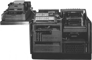
In the early 1960s Lorenz was working at MIT on a Royal McBee LGP-30 (fig. 1). Designed by Stan Frankel and released to market in the mid-1950s, this was by all accounts a cumbersome and slow digital machine, approximately the same size as an office desk, nigh-impossible to boot, and somewhat neglected by chroniclers of the history of computing.Footnote ²⁷ In a 2005 interview, Lorenz could not recall the precise circumstances that led to him having the machine at his disposal, noting simply that “the department gave it to me. . .one day it was there.” What he could recall, however, was the joy of being in control of the modeling process from start to finish.Footnote ²⁸ He was using this machine to investigate finite systems of deterministic ordinary differential equations that were designed to represent forced dissipative hydrodynamical systems. We flag for critical attention what might be meant by “represent” here, for by the time Lorenz's Reference Lorenz1963 paper was published we see a highly simplified model he had adapted of finite amplitude convection in the atmosphere.Footnote ²⁹ Of the multiple configurations of convection that can evolve as air is warmed by the earth's surface, the most simple is a horizontal roll with warm air rising on one side and cool air falling on the other. Lorenz's aim was to model a two-dimensional slice of such a roll, for which some technicalities will be useful. The published convection model went as follows:

Where:

1. 1. The dots on the left hand side signify derivatives with respect to dimensionless time (τ = π²H ⁻² (1 + a ²) kt),

2. 2. X is proportional to the intensity of the convective motion,

3. 3. Y is proportional to the temperature difference between ascending and descending currents,

4. 4. Z is an index of the shape of the vertical profile of the temperature distribution,

5. 5. σ = k ⁻¹v is the Prandtl number,Footnote ³⁰

6. 6. r = R_c ⁻¹R_a, where R_a is the Rayleigh number and R_c a certain critical value of R_a,Footnote ³¹

7. 7. b = 4(1 + a ²)⁻¹.

Fig. 1.

The Royal McBee LGP-30. The approximate dimensions of this “desk” machine, not including the typewriter shelf to the left, are 26 inches deep by 33 inches high by 44 inches long. Immediately above the cooling unit and the digital display unit (marked in the middle of the machine) is the control panel. At top right is the memory drum, and below that lies the power supply: 1,500 watts were needed for operation. Courtesy of the Computer History Museum, Mountain View, California.

Although this is a system of wholly canonical interlocking differential equations, approaching them with pencil and paper would be an execrable business. This is where the Royal McBee had earlier come in. Even if a closed form solution was practically out of reach, numerical integration was not, provided that suitable values had been assigned to the constants. Having set σ = 10, a ² = 0.5 (thus b = 8/3), and r = 28 as plausible empirical values (and with time increment Δτ = 0.01), Lorenz discovered upon running this simulation that it settled down quickly, with X, Y, and Z all taking values within clear limits.

However, if one probed within those limits things were rather less clear: arguably this is our first moment of “seeing differently.” The value of X might oscillate for a given period around positive values, then switch and wander around several negative values, with no discernible pattern governing this “switching” behavior. Similar effects occurred with Y and Z. Lorenz's investigations would quickly furnish even deeper mysteries. At some point before the 1963 paper – Lorenz himself dated the event to the winter of 1961 – he took a shortcut that has subsequently become legend. One particular sequence in a numerical integration grabbed his attention, so rather than re-run the entire experiment he started directly at this point of interest by manually putting in the value from the previous run. Very quickly, and against expectation, this second run diverged from the original, and within a small timeframe bore no resemblance whatsoever to its predecessor.Footnote ³² Lorenz's first intuition was to blame some form of hardware fault, such as a faulty wire or broken vacuum tube, the Royal McBee being prone to breakdown on at least a weekly basis.Footnote ³³ However, after checking out all possible problems and still finding no explanation, Lorenz retraced his steps for this second sequence. The one difference he could find between the initial conditions of the original run and the diverging second run came at a fourth decimal place: he had put in 0.506 for his replication where the original was a more exact 0.506127. This minute difference is what had driven the system off course.

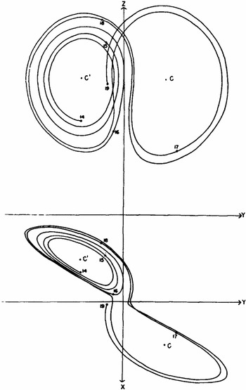
To elaborate the further significance of this experiment, we first note that by the time of his publication Lorenz had charted the three variables of his model through phase space (see fig. 2). Where the X, Y, and Z of the model provide three dimensions through which a trajectory can be traced, Lorenz's model produced a two-looped structure in phase space (a “strange attractor”) that any trajectory will be pulled around regardless of its starting point.Footnote ³⁴ If it were possible to see figure 2 evolving in real-time, one would observe a given trajectory wander around one wing of the structure until it “strays” to a certain point and is thrown towards the other wing. To see the phenomenon of sensitivity to initial conditions (the aforementioned “Butterfly effect”), one could set two trajectories in motion from near-identical points of phase space and, after a suitable passage of time, see them diverge from one another.Footnote ³⁵ Further interesting properties are these: (1) trajectories do not typically repeat, such that there is no overlap whatsoever; (2) the number of turns a trajectory takes around one wing before switching to the other is patternless; and yet (3) the attractor – definable as the set to which a dynamical system evolves after a certain time – has very clear boundaries on a larger scale. Though there is little chance of formulating any globally acceptable definition of “chaos,” this system provides at least one working answer: at the macro-scale, predictability and order; while at the micro-scale, disorder and unpredictability caused by sensitivity to initial conditions.Footnote ³⁶ There is also a sketch using phase space that can motivate a similar idea. Crudely, attractors come about through shrinkage of phase space, while sensitivity to initial conditions involves a spreading apart. What makes the Lorenz system “special” is that we see both at the same time.

Fig. 2.

The Lorenz Attractor. This visualization of Lorenz's three-equation model shows how a trajectory through phase space evolves over time in a complex and non-repeating pattern (Lorenz Reference Lorenz1963, 137). © 2009 American Meteorological Society (AMS)

Moving from a mathematical to a more intuitive or physical sense of the difference between the two runs, a reasonable representation would be adding or omitting a small puff of wind in a real system (or, should one prefer, by adding or omitting the flap of a butterfly's wings). On certain earlier views, small differences in initial conditions would make for correspondingly small differences in output. Sensitivity to initial conditions modified this in a fundamental way: after Lorenz, completely controlling for any divergence in different runs of the model would require the initial conditions of the two runs to be specified with infinite precision – that is, with a precision of which no computer is capable. And if one were attempting to see with certainty the goodness of fit between a model and real world data, then controlling the divergence would require the data to be perfectly precise and noise free – a precision which not even von Neumann or Charney would argue for. Lorenz saw this very clearly in his paper:

Lorenz's result has occasioned no small measure of hyperbole concerning the wholesale death of prediction. Re-reading his original text, we can see that rather more care and nuance are needed. Two states differing by imperceptible amounts may diverge, he claimed. Acceptable prediction may be impossible in the distant future. Thus Lorenz's result does not rule out predictive success in meteorology in general; the force of the argument is more to the effect that the weather cannot be indefinitely predictable.Footnote ³⁷ Putting it another way, predictive success in meteorology will not, given Lorenz's result, look anything like predictive success in a discipline like astronomy (Nebeker Reference Nebeker1995, 192). Yet practically speaking, Lorenz's result only modestly dents dreams of prediction. Meteorological forecast over certain timeframes has, after all, become demonstrably more accurate in the years since Lorenz's result – without complete control over divergence and an apodictic grip on model-data mapping. Nor, more importantly, do we even need grand debates around the death of prediction to distill what is vital for us in Lorenz's intervention. We need only see an epistemological can-of-worms with respect to the stability of models. These cans of worms may frighten one away or they may be taken as an intriguing challenge. In its journey from obscure meteorological journal article to mass consciousness, one group that opted to take on the challenge of Lorenz's model was the DSC.

Kitchen Experiments and the Dynamical Systems Collective (DSC)

The DSC was based at the relatively new campus of UC Santa Cruz between the late 1970s and early 1980s.Footnote ³⁸ Although a broader entourage waxed and waned, the core of the group consisted of four figures: James Crutchfield, Doyne Farmer, Norman Packard, and Robert Shaw. Here we devote most of our attention to work authored by Shaw, but on occasion we shall still use the epithet of the DSC. The reasons for this are not contentious, since the influence of the rest of the group is clearly visible through Shaw's citation practice. Established physicists occasionally win a reference in his work, but the lion's share goes to his PhD colleagues and fellow travelers. The term “collective,” that is to say, was no accident. While the academic credit cycle required that specific names be attached to specific texts, we have the sense that in day-to-day laboratory life it was not always so clear where one person's contribution stopped and another's started.

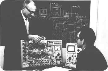
In 1977 Shaw was given the task by his advisor of implementing Lorenz's three-equation model on a Systron Donner machine.Footnote ³⁹ Far from the now familiar set-up of self-contained keyboard and screen, these analog machines presented a façade of patch-panels, coefficient potentiometers, and overload indicators. A vitally important feature of these machines (and, we note, a traditional ground for criticizing them) is that they were frequently “special purpose.” Different models and different systems, that is, could only be made to run by configuring and then reconfiguring various inductors, capacitors, reed relays, trunk lines, variable diodes, and sundry other widgets. With digital computers there is at least some sense in which the computer contains the model or simulates the model. With analog machines, by contrast, the computer to all intents and purposes is the model, working via measured physical quantities rather than counts of discrete units. Thus, “numerical computation” in the sense of von Neumann is sidestepped by the flows of electrons through metal wires.Footnote ⁴⁰

A less esoteric picture of these machines, and one that sheds rather more light on the question of their use, can be constructed from two sources. First, we provide figure 3, which is a detail from the cover of a Systron Donner pamphlet first put out in 1968, showing what the machines physically looked like (not to mention inserting an intriguing presumption as to who the end users might have been). Secondly, we wish to reintroduce Yoshisuke Ueda. His name was briefly mentioned above as one doing important work on chaos in the early 1960s. On the question of using an analog computer, Ueda provides a concreteness that, while certainly not generalizable in every detail, lays bare the extent of tinkering required. Discussing the analog machine built by his colleague Minoru Abe, and which Ueda used in his investigations of mixed van der Pol and Duffing equations, he describes what was then business as usual:

While this is a lovely quote as regards tinkering, we should mention that Ueda certainly did not miss the analog machine once digital resources became available. Describing analog computing as “extremely cumbersome,” “infernally long,” and “not reliable,” he goes on to note: “What more or less saved us was the new digital computer KDC-1, which had just come out” (ibid., 59–61). We will show in due course that at least on some occasions there were reasons to demur from such judgment, but for now we want to insist on the extent to which the practice of the DSC represents a mode of computational tinkering: far more “grubby engineering” than “elegant physics”; far more “hacking” than “planning” (Turner Reference Turner2006, 133). They were not passive end users of black boxes, but rather chopping and tweaking in a way almost as easy to associate with radio amateurs or electronic musicians as with “serious” computing professionals.Footnote ⁴¹ As Heinz Pagels wrote with a telling deployment of scare quotes: “I recall visiting their ‘lab’ back in 1981 and thinking that most of their equipment came out of the local hardware store. They had a hard time convincing their colleagues that they were doing something important” (Pagels Reference Pagels1988, 81).

Fig. 3.

Depiction of a Systron Donner analog computer. With analog machines, computations are performed using such properties as electrical resistance and voltage. Courtesy of the Computer History Museum, Mountain View, California.

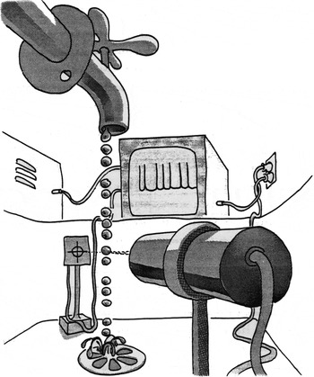
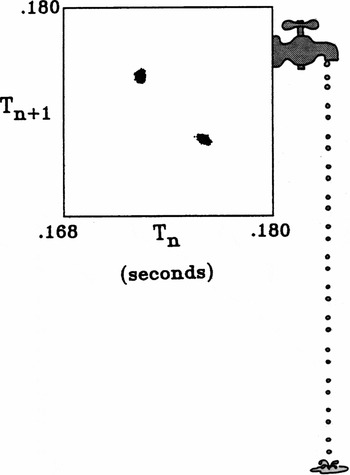
There are several levels to attend to in this episode. The way that their “lab” deformed the usual set-up of equipment, we find, came hand in hand with further deformations, from the very format of presenting results through to deformations at the conceptual level. To bring this out more fully, we now move to a close reading of Shaw's intriguing 1984 monograph, “The Dripping Faucet as a Model Chaotic System.” Stylistically, the piece is a model of clarity, the text composed in a crisply distilled manner familiar from the high-end scientific journal. Yet this is not work intended for any such arena. Alongside exposition of experimental results one finds both philosophical speculation and sometimes vigorous critique of the scientific establishment. The very look and feel of the piece deliberately eschews any standard way of doing things: the font is clearly straight from a typewriter, many equations and even textual corrections were put in by hand, and the reader is helped along throughout by the cartoons of Chris Shaw, Robert's brother. Figure 4 presents one of the more important cartoons for our purposes, illustrating an experimental apparatus in which a photocell signal reads off the time intervals between successive drops of water.

Fig. 4.

The Dripping Faucet System. Drops falling from the faucet at top left break a light beam, which produces pulses in a photocell signal. The pulses in turn operate a timer with a resolution of 4 microseconds that produces the basic data: time intervals between drops (Shaw Reference Shaw1984, 3). © 2009 Aerial Press

Even without any oddities of presentation, it may seem that the very choice of problem is rather bizarre – especially coming at a time when physics experiments are imagined to offer windows onto minute length scales via mile-long accelerators. Part of the task we face is to show why this conclusion can be resisted for an experiment described by its own author as “well worth performing in the privacy of one's own kitchen” (Shaw Reference Shaw1984, 2).

We begin by paraphrasing Shaw. He notes that for a classically trained physicist, modeling the dripping faucet might involve (1) writing down the equations of motion; (2) writing down the coupled differential equations describing fluid flow and the forces of surface tension; and then (3) solving them with appropriate boundary conditions (ibid., 4). Even for a simple system, however, this is an approach of forbidding difficulty.Footnote ⁴² Shaw's response to this was striking: “Another. . .approach is to. . .forget the physics entirely, and view the system as a black box producing a stream of numbers t_1, t_2, t_3, . . .in this case the drop intervals” (ibid., 5).Footnote ⁴³

The structure embedded in this stream of numbers turned out to be far from banal, but innovative work was needed to draw out what the unaided eye or ear could all too easily miss. In order to visualize the single dimension of data coming out of the black box, Shaw introduced the so-called “time versus time” map in which T_n was plotted on the x-axis and T_n+1 on the y-axis.Footnote ⁴⁴ The easiest example for building intuition is for low rates of flow that have a strict periodicity – in simple terms, drops falling with identical intervals between them. The time-versus-time map corresponding to this would cluster around a single point in two-dimensional space. As the flow rate was increased, however, Shaw began to note variations in the drop interval, which continued up until a period doubling bifurcation. At this point two drops had to fall before the system behavior repeated itself; the time-versus-time map for this scenario is given as figure 5.

Fig. 5.

A time-versus-time map for the period 2 regime of the dripping faucet. Period doubling is the best known “route to chaos”: first comes period doubling (in this case, two drops before the system behavior repeats itself), then quadrupling (four drops before repetition), and so on until the onset of chaos (Shaw Reference Shaw1984, 8). © 2009 Aerial Press

The notion of bifurcation is an important one to grasp, and can be glossed as the sudden appearance of qualitatively different behavior in a nonlinear system as some parameter is varied. The dripping faucet system, while simple, was nonlinear exactly insofar as the detachment of the drop at T_n+1 was influenced by an interaction with the drop at T_n. And if one drives such nonlinear systems harder and harder – for Shaw that simply meant opening the faucet more and more – such bifurcations recur, with richer and richer structure coming into view until one sees the onset of chaos.

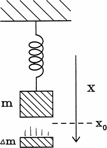
With at least a working idea of the experimental system and the data it produced, we now turn to consider the model that Shaw proposed to mirror his data – implemented, once again, on an analog computer. To obtain a mental picture, one can imagine an individual water drop to be represented by a mass that grows linearly in time (see fig. 6). This stretches a spring (equivalent to surface tension in the real system), and when the spring is stretched to a specified length the mass drops off suddenly by an amount dependent on the speed of the mass at critical distance (equivalent to a drop detaching). This gives the following: “A driven nonlinear oscillator, the nonlinearity arising from the sudden change of mass, and with position, velocity, and mass providing the three variables required for the occurrence of chaotic behavior in a system evolving in continuous time” (ibid., 15).

Fig. 6.

Shaw's model of a water drop at low flow rate. A spring bearing a mass (m) is stretched linearly until at a certain distance the mass “falls off” by Δm as a drop detaches (Shaw Reference Shaw1984, 15). © 2009 Aerial Press

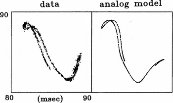
Given the evident simplicity of the model – Shaw himself termed it “naïve” – the correspondence obtained between streams of system data and model output was striking. As can be seen for a higher flow rate, displayed for instance in figure 7, the real system data proved a little noisier – a matter we shall return to in our section on the plasticity of error. Still, in spite of the noise both the structural richness and tight correspondence between system and model – especially when imagined against the undifferentiated mess that a genuinely random system would produce – is quite unmistakable.

Fig. 7.

A time-versus-time map comparing dripping faucet system data with the “naïve” analog model (Shaw Reference Shaw1984, 16). © 2009 Aerial Press

To conclude this section, we enter a brief note for those who may have read our first paper in this issue. There it was clear that Forrester was not hugely concerned with model-data correspondence, just so long as the overall behavior of the model was appropriately realistic. Here, by contrast, not only is model-data agreement (if not forecasting) a live consideration, but it also functions as a springboard to further questions about chaotic systems. Shaw, that is to say, aimed at far more than producing a model that could ape key features of faucet data streams at certain parameter values. He wanted instead to use his low level system to then transition into the topic of “modeling in general.” As Shaw put it in a rather apologetic passage, “I hope the reader can forgive the loose tone of some of [the] discussion, and that if it is not science, it is at least entertainment. Perhaps, though, contemplation of a dripping faucet can supply a few rungs in the ladder of metaphor which must be built to understand modeling in a larger sense” (ibid., 97; our emphasis). In our next section, we will endeavor to unpack just what Shaw had in mind here.

From Kitchen Experiment to Models in General

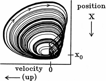
One way of moving from the faucet to models more generally is quite immediate: the dripping faucet model shared important structural features with a broader class of models. As Shaw himself made plain, one of the comforting features of “the nonlinear jungle. . .[is that] certain landscapes tend to reappear. In the dripping faucet system we have recognized forms and bifurcation sequences common to [other] low-dimension models” (ibid., 14). One good instance of this is the presence of the Rössler attractor (named after German biochemist Otto Rössler) in its so-called “funnel” regime. The attractor was first derived theoretically and then later used to model chemical kinetics (Rössler Reference Rössler1976; Rössler Reference Rössler1979). To tie this to the dripping faucet system, we first note a small model-to-data translation problem: the analog model of the faucet introduced continuous variables that were not shared by the particular experimental set-up. This addition proved useful, however, exactly insofar as it helped to visualize the overall geometry of the attractor describing faucet system motion. In what will hopefully function as a “eureka” moment, this attractor turns out to bear exactly the same geometry as Rössler's, despite coming out of a totally different experimental context in which a wholly different set of equations were used (see fig. 8).

Fig. 8.

The Rössler Attractor. Rössler's original paper makes plain a certain family resemblance between his structure and the Lorenz attractor given as Figure 2 above. In particular, it shares the same tracing of trajectories over finite values but with chaotic oscillation (Shaw Reference Shaw1984, 17). © 2009 Aerial Press

This is already a powerful result, and Shaw gave several more to consider. The faucet system could also provide a more general lesson about modeling insofar as it presented limits on predictability. Shaw's rendering of prediction loss for the faucet, drawing on earlier work by Claude Shannon, was in terms of a loss of information. This rendering required a little re-interpretation of Shannon's work. Originally, Shannon had modeled information loss in a communication system consisting of a transmitter and a receiver that were connected to each other by a channel. To serve Shaw's purpose in dynamical systems, however, the word “system” was reconstrued as any body of information transmitted through time by dynamical variables. Thus, Shaw thought not of a transmitter but the past state of a system; not of a receiver but the future state of a system; and not of a channel but the system dynamics that connects past to future (Shaw Reference Shaw1984, 37).

Earlier we promised to show that Shaw's kitchen experiment is far from a bizarre choice of problem, and are now in a position to give our strongest reply. A charitable elaboration of Shaw's faucet work, we argue, in all its anti-glamor and with all its “special case,” “low-tech,” and “obsolete” equipment, forces one to face head-on the following crucial questions about modeling chaotic systems in general: “Given a stream of data, how much can we infer about the system that produced it? What sort of measurements should we make to optimize the predictability of a system? Do we use the same criteria to best determine the past states of a system?” (ibid., 68).

The answer Shaw gave to these questions is that one must constantly walk on a razor's edge, measuring and compiling data for histograms that are at once wide enough to get “nice” numbers, yet narrow enough to get “out of the noise” and capture as much of the deterministic dynamics as possible. In terms of what one might hope for even with a very simple chaotic system, Shaw's view was less than encouraging: “Data records taken so far, typically of length of four to eight thousand drop intervals, are in fact only marginally able to satisfy both these conditions simultaneously, even for the simple attractor used as the main example. Also, the noise level below which no causal structure exists is to an extent an assumption, a judgment on the part of the experimenter” (ibid., 84).

With Lorenz and the DSC, the dream of what might be called “ultimate predictive modeling” receives a heavy blow. Our first paper showed that Forrester was simply too pragmatic to be tempted by the picture in which a large enough brain could hope to produce the “right” model – “right” being construed along the lines of “maximally faithful to past and future experimental data.” Instead, he wished for his students to start out with a model that could reveal qualitatively interesting behavior and then iteratively improve it in a way that was heavily dependent on the task at hand. The work of Lorenz and the DSC sets up a stronger conclusion than this:

With chaotic systems, then, one might not even know when the optimum model of chaotic systems has been attained, in the sense of knowing sharply when the limit to predictability has been reached.

Styles of Modeling and Technological Use

So much for the fine grained details of actual models; we now turn to the part of our argument addressing the idea of an “adequate” technology with which to model in the first place. We begin by digging into some purported differences between analog and digital computing. In certain circles it has become fashionable to view analog computing as a thankfully redundant pastime quite justifiably overthrown in the war with digital (for a survey of and critical response to such views, see Owens Reference Owens1996). This could lead in the first instance to a rather strange picture of the DSC, simultaneously forward-looking with respect to its intellectual agenda and yet backward-looking in its membership in an “old” computer regime.Footnote ⁴⁵ One resolution of this oddity could be simply to explain it away. That the DSC was using analog apparatus so late in the day might, on such a view, reflect such contingencies as the group's fringe status and consequent inability to pull in funding that could have made for more sophisticated (read: digital) experimentation. We find that this strategy of explaining away will carry us at least a short distance. After all, the DSC made explicit reference both to failed NSF funding applications and to the pleasingly low cost of analog machines. Moreover, the use of analog machines was not programmatically exclusive. When the opportunity to use a donated digital machine presented itself, the DSC certainly did not turn away in horror, and at least one author has sketched DSC member Doyne Farmer as constantly on the lookout for free computer time – one presumes on digital machines (Gleick Reference Gleick1987, 241–272).

However, we feel that approaching this oddity exclusively in the mode of explaining away is not satisfactory. To begin with, this approach risks smuggling certain notions of “typicality” through the back door. When reading accounts of how the analog / digital “dialectic” played out, it is common to see examples such as wartime ballistics used as a typical reference frame that sets the rules for sound practice thereafter. One classic victim of this narration is the differential analyzer, a wheel-and-disc analog machine conceived in the later decades of the nineteenth century and realized by Vannevar Bush and H. W. Nieman, both at MIT, between the late 1920s and early 1930s. Over the course of World War II, two of these analyzers were used to compile ballistics tables at the Aberdeen Proving Ground.Footnote ⁴⁶ Herman Goldstine, a Professor-turned-Lieutenant at Aberdeen (and later co-director of the ENIAC project), arrived at a rather dim view, noting that the best analog machines were only “about 50 times faster than a human with a desk machine. None of these [machines]. . .were sufficient for Aberdeen's needs” (Edwards Reference Edwards1996, 49; our parenthetical addition). However, even if one allows that computing ballistics tables using analog technology was tedious and difficult, and that the attempt to install digital computing for ballistics tables was technologically dictated,Footnote ⁴⁷ tweak both the context and style of work and things rapidly look very different. Here is an insight from Doyne Farmer:

From a dynamical systems viewpoint, then, the analog machine at Santa Cruz turned out to be suited to its purpose in quite fundamental respects – a certain form of technology lent itself admirably to a certain style of computing. The analog computer made the adjustment and exploration of parameters a matter of simply tweaking knobs “on the fly” and then intuitively “zoning in” on regions of interest, thus opening up an avenue of quick and real time virtual experimentation.Footnote ⁴⁹ Shaw made perhaps an even stronger claim, namely that his hybrid program of research called for machines of corresponding hybridity. The sentiment ran deep enough to be explicitly mentioned in print:

Here, analog technology is endorsed out of an interesting mix of practical virtue (notably speed) and epistemological virtue (utility in modeling systems where qualitative understanding is lacking). The choice of technology hinged on the type of model Shaw wanted to build and use to generate a particular type of experimental knowledge. Of course in some sense it must be conceded that these analog machines offer less than the von Neumann gold standard of precision.Footnote ⁵¹ And yet it seems quite irresistible to argue for alternative standards being built here, in which the very meaning of “appropriate” technology morphs as a function of the epistemological task at hand. We thus suggest a need for considerable caution in recycling any opposition of imprecise and error-ridden analog to obviously better digital.Footnote ⁵² In the face of differing styles of computing and modeling – that is to say in the face of orthogonal modes of practice – this way of thinking quickly loses traction. And in the face of orthogonal modes of practice, orthogonal ways of thinking epistemologically follow. With that we turn to consider what might be said about the notion of error in light of our cases above.

Stability and the Plasticity of Error

Over the longer history of chaos, retaining pre-conceived notions of stability has played a thorny and complicating role.Footnote ⁵³ Arguably the first case where difficulties arose came with Poincaré's late nineteenth-century work on celestial mechanics, which many scholars have taken to provide the first ever glimpse of chaos. As part of the 60th birthday celebrations for King Oskar II of Sweden, a prize was announced that would go to whoever showed the solar system – as modeled by Newton's equations – to be dynamically stable. Put another way, the prize would go to whoever could solve the three-body problem. Famously, Poincaré did not solve the problem but nevertheless took the prize for his attempt, finally published in 1890 after a few rounds of editorial jitters and much behind-the-scenes intrigue. The paper showed that in fact three bodies would trace different paths after starting from only slightly different initial conditions – essentially a discovery close to the one that we attributed here to Lorenz. This is not mere carelessness on our part. Rather, the care needed is in making any priority claim for Poincaré, for even if chaos had been glimpsed as a phenomenon it was certainly not recognized as such. Poincaré's commitment to the idea of a stable solar system would persist, arguably in spite of his own work rather than because of it (Poincaré Reference Poincaré1890; Galison Reference Galison2003).

Poincaré would not be the last in the history of chaos to encounter these bizarre moments of system instability. In the summer of 1953, after a year of planning, Enrico Fermi, John Pasta, and Stanisław Ulam used the MANIAC computer at Los Alamos to investigate a one-dimensional system of 64 particles in which the connections between neighbor particles were nonlinear.Footnote ⁵⁴ Their expectation was that after a certain time the system would display first “mixing” and then “thermalization,” essentially a settling down behavior in which the influence of the initial modes of vibration in the system would cease to be visible. And at least in the beginning they got what they wanted – the initial simulations on MANIAC conformed very well to intuition. However, on one occasion the simulation was left to run longer than intended, at which point a deep curiosity came into view. Rather than progressing smoothly towards a steadier and steadier state caused by the gradual sharing of energy, the system would suddenly reassemble itself into a state similar to the initial conditions. The system was then left a little longer and showed more behavior in the vein of jumping around than in settling down. From this, the authors concluded, “the existence of quasi-states may be conjectured,” but no deeply satisfying framing would be found before Fermi's death the following year (Fermi et al. Reference Fermi, Pasta, Ulam, Edoardo, Anderson, Persico, Segrè and Wattenberg1965).

Where Poincaré wanted stability, one might say, Fermi and coworkers wanted smoothness. On the other side of the coin for all the actors lay error, in the near-etymological sense of “wandering away” from that which is right. This aversion to the unstable, the jumpy, and the wandering was also importantly shared by von Neumann. We have written above of his efforts to intertwine meteorology with large scale computing; to these two activities we may also add a third salient thread of his contributions to numerical analysis. The most germane paper to consider here is “Numerical Inverting of Matrices of High Order,” co-authored with Herman Goldstine in 1947. Here, and very much consistent with his thinking about meteorology, securing stability was again set up as an overriding aim. The question of rounding limitation in computing was parsed in the paper as an inherently bad thing – an objective deficiency, an evident obstacle in coming to know, and precisely what one should seek to screen off and manage. The epistemic force of this aversion has not dissipated in more recent times. In 1993, for example, Jean-François Colonna conducted an experiment in which five algebraically equivalent formulae for Verhulst dynamics produced different results – errors, even for innocuous parameter values – because of limited floating point accuracy on different digital computers. When Colonna, as a consequence of this finding, spoke of the “subjectivity of computers,” it is hard to imagine this having any particularly positive connotation. This suspicion is confirmed by his concluding remarks: “Today, when both fundamental and applied research relies so heavily on computers, it is essential that users (engineers, scientists and students) should be perfectly aware of the dangers, and that efforts should be made to find real solutions to this very real problem, if such solutions exist” (Colonna Reference Colonna1993, 18).

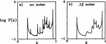
Against this historically rather strong aversion, we urge that our conclusions about practice and the notion of “adequate” technology – essentially that any such adequacy be always read against the task at hand rather than any absolute standard – feed through here to produce an epistemological conclusion regarding the status of error. In the Lorenz study, rounding limitation almost accidentally became the cause of massive illumination. Through what could be described as error, Lorenz saw that vanishingly minute differences between two systems of a completely deterministic stripe can nevertheless result in exponentially diverging trajectories. This, we think, gives rounding error a different and indeed intellectually illuminating resonance.Footnote ⁵⁵ The argument can be extended further with a consideration of the DSC's analog machine. Again, in tandem with a certain style of modeling deployed for a specific task, we find there is no compulsion to accept any picture concerning the “redundancy” of an “error-ridden machine.” The notion of error and precision have instead to be relaxed and seen as somewhat plastic for this particular context of chaos experiments. If we absolutely insist on rigidly sticking to the notions, then – we think rather perversely – it is precisely the error and imprecision of the analog computer that does such sterling work for the Santa Cruzans. This much is very well captured by Gleick: “Shaw. . .would set the [system's] initial conditions, push the go button and off the attractor would go. Then he would set the same initial conditions again – as close as physically possible – and the orbit would sail merrily away from its previous course, yet end up on the same attractor” (Gleick Reference Gleick1987, 246–247). Gleick is discussing the DSC implementation of the Lorenz model here, but advantageous use of imprecision also played a role in the faucet experiment. There, one possible model considered for the system data was the parabolic map with noise added, x´ = rx (1 – x) + ζ, where ζ is a random variable of small width (Shaw Reference Shaw1984, 55). We begin by referring the reader to figure 9, which shows two invariant distributions P(x) for this map, with r set to 3.7.

Fig. 9.

Invariant distribution with and without noise added. This gives a map of the values and probabilities that a given event may have (Shaw Reference Shaw1984, 55). © 2009 Aerial Press

In explaining how the two graphs were drawn, Shaw made the following crucial remark: “Here the ‘noise’ uncertainty is modeled for convenience by a simple truncation of the accuracy of the computation. . .The experience of Crutchfield and Packard and others has been that the outcome of numerical experiments such as this is usually unaffected whether one takes ζ to be of Gaussian, uniform or other form. Only the effective width of ζ is important” (Shaw Reference Shaw1984, 56).

In building this particular model, then, the inaccuracy of the computer was deliberately used as a tool for capturing some of the sensitivity in the actual system. All this serves to make plain some substantial transformations of the same phenomenon when ported to different cantons. When Paul Edwards looked back to the time of von Neumann and told us that World War II “nearly drowned in the noise of its own technology,” the negative connotation of noise and imprecision could not be clearer, and, as we have shown, von Neumann did all he could to screen this off (Edwards Reference Edwards1996, 210). Noise and error in this context are bywords for deficiency, for something going wrong that will impede scientific progress. With Lorenz's work on sensitivity to initial conditions, the connotation of imprecision changes, and the story cannot be articulated without some reference to the pseudo-serendipitous moment made possible by an “imperfect” computer.Footnote ⁵⁶ Switch once more to the dripping faucets of Santa Cruz, and again the connotation of noise mutates. On occasion they positively wanted noise rattling around their models, and deliberately used it as a tool. In this ecology, round-off error is not that which must be eliminated, but rather that which is knowingly used in fruitful research.Footnote ⁵⁷

Series Conclusion

In drawing this two-part work to a close, we wish to summarize what the main points of continuity and difference are in following our discussion all the way from Forrester through to the Dynamical Systems Collective. With respect to continuity, the actors in our two papers share an interest in doing something at times quite orthogonal to the practice of modeling for prediction and forecast. In all the cases we have examined, it was important to have models that imbued the user with understanding of certain systems, teaching them how to see differently. New epistemological possibilities came hand in hand with new practices of computing and modeling. It is not enough simply to postulate a facilitation of certain kinds of work by certain kinds of pedagogy or technology; what we have done instead is to begin to provide an articulation of how and why this occurs.

Yet all is not commonality and red thread. We close, then, by recapitulating what is distinctive about this paper with respect to its predecessor. First, there is a notable distinctness in the behavior of the systems treated in our respective papers, a distinctness that brought with it crucial implications for how the models were built, used, and thus may be analyzed by the historian or philosopher of science. We recall that Forrester's model-building process was necessarily iterative. Intermediate models had to be studied and tested for plausibility and robustness before moving on to scenarios where expectation and intuition were not so clear. His was an approach of edging ahead, of building more sophisticated models off the back of their less sophisticated forebears until a suitable structure – suitable in the sense of providing instructive behavior – eventually emerged. With chaos, things are different. Even in the very easiest cases – such as the well-known logistic equation for population growth – and certainly for the convection and dripping faucet models examined here, suddenly upping the value of a parameter can at one moment make no qualitative difference and at another moment drive the system into a totally new regime of behavior. One does not see actors piling iteration upon iteration, or constantly adding new modules to ever-complexifying models. This is not to say that either Lorenz or Shaw had “golden models” from the outset: that would be quite fatuous. Yet their models were still pared down to a point of great simplicity compared to Forrester's, with structure coming into and fading out of view via the adjustment of specific parameters. Lorenz was to some qualified degree “lucky” to derive this behavior from his model, but with the systematic study of information loss by the DSC it was quite crucial to be able to scan blindly over different parameter values and “interrogate” or “zone in” on regions of interest; a process far less to do with weltbild and more to do fingerspitzengefühl, as Kaiser would have it (Kaiser Reference Kaiser2005, 8). This orientation towards fine-grained parametric detail does not obtain in Industrial Dynamics.Footnote ⁵⁸ Modeling the faucet was less about overall robustness in modeling a scenario and more about probing particular sensitivities in a simulation. It was absolutely crucial to be able to tweak knobs with settings, but ironically not because this brought with it any guarantee of precision. With certain pre-ordained and overly rigid notions of error in mind, this last remark may sound paradoxical. We hope to have shown it need not be. With Bachelard, we claim that “each interesting problem, each experiment” – and to this list we venture to add “each model” – “requires a philosophical reflection of its own” (Rheinberger Reference Rheinberger2005, 317).Footnote ⁵⁹ This is a pluralism that seems unexceptional when applied from the present to the more distant past, yet for it to appear so required much work. C. S. Lewis is a fitting figure to conclude with. In The Discarded Image one finds a masterful and sympathetic rendering of the medieval model of the cosmos. Indeed, so great is the sympathy that the author himself seems almost worried by it:

As for Lewis in his vertical jump to the Medieval from the Modern, so for us in our horizontal jump across different but near-contemporary sites of model making. We offer no metric for “right” and “wrong” modeling here, and nor do we think this to be useful. The plasticity of error in chaos experiments rules out any easy narrative pitting error against truth, and what emerges as epistemologically important or technologically adequate depends heavily on difference in styles of computing and modeling. This we also see as not only pardonable but inevitable. Does this leave anything beyond a vanishing particularism? We believe so. What we have established in our papers is a set of useful concepts – structure versus parameters; robustness versus predictability; problems of complexity versus problems of sensitivity; iterative construction versus continual interactivity; heuristic, pedagogical, and exploratory modes of use; result versus behavior – all of which we think to be essential to understand in developing further critical thinking about the history and philosophy of computer simulation.