1. Introduction
Cross-flow instability is a primary mechanism for the breakdown of the laminar flow and onset of transition in three-dimensional swept wing boundary layers. The disturbance is inflectional and is therefore susceptible to the inviscid instabilities examined by Gregory, Stuart & Walker (Reference Gregory, Stuart and Walker1955). Taking the form of stationary co-rotating vortices (and travelling disturbances), cross-flow has been observed on rotating discs and cones by Kohama (Reference Kohama1984) and Malik (Reference Malik1986), amongst many others.
Many experimental and theoretical investigations have been undertaken concerning the various stages of the cross-flow vortex development on swept wings. Using a swept wing model with an imposed pressure gradient, Müller & Bippes (Reference Müller and Bippes1988) observed both stationary cross-flow vortices and travelling wave disturbances prior to the onset of nonlinear saturation. Kohama, Saric & Hoos (Reference Kohama, Saric and Hoos1991) identified a high-frequency secondary instability before the onset of transition. Linear and nonlinear theoretical investigations of three-dimensional boundary layers were carried out by Meyer & Kleiser (Reference Meyer and Kleiser1988) using direct numerical simulations of the Navier–Stokes equations, while Fischer & Dallmann (Reference Fischer and Dallmann1991) applied a secondary instability analysis. Malik, Li & Chang (Reference Malik, Li and Chang1994) conducted an investigation of the linear, nonlinear and secondary instability stages of the cross-flow evolution and the laminar–turbulent transition mechanisms in the swept Hiemenz flow. Their analysis was based on a system of nonlinear parabolized stability equations (NPSEs). Both the stationary and travelling cross-flow disturbances were examined. Detailed descriptions of the vortex development, inflectional velocity profiles and the generation of the so-called half-mushroom structures were discussed. A high-frequency secondary instability was observed prior to the onset of transition, agreeing with the earlier experiments on a swept cylinder by Poll (Reference Poll1985) and swept wing by Kohama et al. (Reference Kohama, Saric and Hoos1991). Similarly, in the rotating-disc boundary layer, theoretical and experimental observations of a high-frequency secondary instability have been identified by Kohama (Reference Kohama1984) and Balachandar, Streett & Malik (Reference Balachandar, Streett and Malik1992), respectively. Further investigations concerning the development and control of secondary instabilities have been undertaken by Janke & Balakumar (Reference Janke and Balakumar2000), Koch (Reference Koch2000), Wassermann & Kloker (Reference Wassermann and Kloker2003), Bonfigli & Kloker (Reference Bonfigli and Kloker2007), Friederich & Kloker (Reference Friederich and Kloker2012) and Obrist, Henniger & Kleiser (Reference Obrist, Henniger and Kleiser2012).
Transition prediction in swept wing configurations is generally based on the
 $\text{e}^{N}$
methods that relate the onset of transition with the logarithmic amplitude ratio
 $N$
of the most unstable linear disturbance. Although this approach has many benefits and is implemented by both the academic and industrial communities, it is based only on linear stability analysis and does not take into account the nonlinear effects, secondary instability or the initial amplitude of the disturbance within the boundary layer. Experimental measurements by Reibert et al. (Reference Reibert, Saric, Carillo and Chapman1996) demonstrate that, in order to predict transition accurately, it is necessary both to consider the initial flow properties of the boundary layer disturbance and to include the nonlinear development of the primary instability. Using NPSE methods, Malik et al. (Reference Malik, Li, Choudhari and Chang1999) generated a velocity profile for secondary instability analysis and found that the development of the stationary vortex agreed with the earlier experimental studies. The growth and frequency of the secondary instability prior to transition was consistent with the respective findings of Kohama et al. (Reference Kohama, Saric and Hoos1991) and Kohama, Onodera & Egami (Reference Kohama, Onodera, Egami, Duck and Hall1996). Malik et al. (Reference Malik, Li, Choudhari and Chang1999) describe an
 $N$
factor transition prediction method based on the secondary instability analysis that may be more efficient than a scheme that is reliant on the linear analysis
Environmental factors can filter into the boundary layer near a solid surface, seeding steady and unsteady fluctuations of the basic state. This process is known as boundary layer receptivity (Morkovin Reference Morkovin and Wells1969) and characterizes the initial stages of the breakdown of the laminar flow. External causes for receptivity can be attributed to the flow interacting with free-stream acoustics, turbulence, vortices and wall deformations, including surface curvature, discontinuities and roughness (Saric, Reed & Kerschen Reference Saric, Reed and Kerschen2002). Receptivity of the boundary layer establishes the initial conditions for the amplitude, frequency and phase of the disturbance within the flow.
If the initial amplitude of the perturbation remains relatively weak, the path to transition is driven by the excitation and development of a primary modal instability: Tollmien–Schlichting (TS) waves on a flat-plate geometry and cross-flow on swept surfaces. Modal growth of the initially small-amplitude disturbance can be computed using linear stability theory, but as the magnitude of the TS wave or cross-flow instability grows, nonlinear processes are amplified through modal interaction with the higher-order harmonics. This in turn can lead to the generation of secondary instabilities and transition (Herbert Reference Herbert1988; Saric, Reed & White Reference Saric, Reed and White2003).
For the current investigation, our interest concerns the receptivity of cross-flow disturbances within the swept Hiemenz boundary layer that develops through both the linear and nonlinear stages of the laminar–turbulent transition process. Cross-flow disturbances are excited using two wall forcing schemes: a periodic suction and blowing strip, and a band of periodic holes with constant suction or blowing. The form of cross-flow generated by the wall forcing is then characterized by several initial flow properties, including the Reynolds number, spanwise periodicity and time–frequency. Further, the shape, location and size of the forcing influence the amplitude of the disturbance and can significantly affect the onset of transition. When the initial amplitude of the disturbance is relatively weak, linear stability theory is implemented to compute receptivity. Given this assumption, it is sufficient to decompose perturbations in the form
 $$\begin{eqnarray}q(\boldsymbol{x},t)=A_{c}\tilde{q}(\boldsymbol{x},t),\end{eqnarray}$$
where
 $\tilde{q}$
specifies the linear growth and the spatial–temporal evolution of the instability, while
 $A_{c}$
is a constant defined as the initial or receptivity amplitude of the disturbance. When wall roughness is responsible for the excitation of perturbations, the size of
 $A_{c}$
has been shown by Streett (Reference Streett1998) and Mughal (Reference Mughal2012) to vary significantly with the shape, height and localized distribution of the surface imperfection. If the initial size of the perturbation is relatively small, the linear stages of the disturbance development can continue far downstream of the prescribed wall forcing. However, as the magnitude of the initial forcing and amplitude
 $A_{c}$
increase, the appearance of nonlinear effects and transition are promoted.
Theoretical investigations concerning the receptivity of three-dimensional boundary layers to wall roughness have been undertaken by Federov (Reference Federov1988), Choudhari (Reference Choudhari1993, Reference Choudhari1994), Crouch (Reference Crouch1993) and Ng & Crouch (Reference Ng and Crouch1999). Receptivity to wall roughness on a curved aerofoil in a compressible flow was investigated by Collis & Lele (Reference Collis and Lele1999) by solving the linearized Navier–Stokes equations. Wassermann & Kloker (Reference Wassermann and Kloker2002) developed a vorticity formulation to examine the effects of nonlinearity in the incompressible flow over a swept flat plate. Studies by Schrader, Brandt & Henningson (Reference Schrader, Brandt and Henningson2009) and Schrader, Amin & Brandt (Reference Schrader, Amin and Brandt2010) considered the receptivity of the flow over a swept flat plate to free-stream turbulence and wall roughness. Spalart (Reference Spalart, Arnal and Michel1990) generated cross-flow vortex structures using disturbance inputs at the attachment line that characterized random noise, waves and wavepackets. Further studies concerning receptivity have been undertaken by Hunt & Saric (Reference Hunt and Saric2011), Tempelmann, Hanifi & Henningson (Reference Tempelmann, Hanifi and Henningson2012a ), Tempelmann et al. (Reference Tempelmann, Schrader, Hanifi, Brandt and Henningson2012b ), Hosseini et al. (Reference Hosseini, Tempelmann, Hanifi and Henningson2013) and Lovig, Downs & White (Reference Lovig, Downs and White2014).
A vorticity formulation developed by Davies & Carpenter (Reference Davies and Carpenter2001) is utilized and is extended to include the effects of nonlinearity on cross-flow receptivity in the swept Hiemenz flow. Using the results of both the linear and nonlinear receptivity studies, relationships are sought that characterize the following flow properties.
-
(i) The effect of nonlinearity on the size of the disturbance, both locally about the centre of forcing and during the modal development of the cross-flow instability.
-
(ii) The onset of nonlinear saturation, where the linear and nonlinear disturbance computations are significantly different.
-
(iii) The location at which the primary Fourier harmonic of the chordwise velocity disturbance first attains a stationary point or maximum.
-
(iv) The size of the physical disturbance about this location.
Details of the nonlinear extensions to the vorticity system of equations are included in the following section along with a description of the basic state. The numerical methods and computational parameter settings used to accurately and successfully generate cross-flow are defined in § 3. Definitions for the amplitude of the cross-flow disturbance, the onset of nonlinear saturation and the chord location at which the primary Fourier harmonic of the chordwise velocity attains a stationary point or maximum are given in § 4. In § 5 the receptivity of cross-flow to various initial forcing distributions is discussed; and final remarks are given in § 6.
2. Formulation
2.1. Swept Hiemenz flow
Consider an incompressible viscous fluid in a Cartesian coordinate system
 $\boldsymbol{x}^{\ast }=\{x^{\ast },y^{\ast },z^{\ast }\}$
relative to a swept plate, where
 $x^{\ast }$
and
 $y^{\ast }$
respectively denote the chordwise and spanwise flow directions. The
 $z^{\ast }$
axis specifies the direction normal to the wall. Uniform flow fields
 $U_{\infty }(x)=mx^{\ast }$
and
 $V_{\infty }$
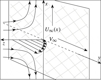
are directed along the chordwise and spanwise axis, engineering the swept Hiemenz flow that impinges on an inclined plate. (Refer to figure 1 for an illustration of the described flow.) The flow is symmetric about the attachment line
 $x^{\ast }=0$
, and for given conditions is susceptible to the disturbances investigated by Hall, Malik & Poll (Reference Hall, Malik and Poll1984) and Spalart (Reference Spalart1988). Further along the chord, the flow is unstable to cross-flow vortices, which have been studied for their linear and nonlinear stability characteristics by Malik et al. (Reference Malik, Li and Chang1994), amongst others.
Illustration of the swept Hiemenz flow, depicting the streamlines in the chordwise
 $x$
direction and sweep velocity along the spanwise
 $y$
direction.

Units of length are scaled on the typical thickness parameter
 ${\it\delta}=\sqrt{{\it\nu}/m}$
for
 ${\it\nu}$
the kinematic viscosity of the fluid. The corresponding velocity components are dimensionalized using the spanwise flow field
 $V_{\infty }$
. Hence, the non-dimensional coordinate system and the undisturbed velocity are defined as
 $$\begin{eqnarray}\boldsymbol{x}=\boldsymbol{x}^{\ast }/{\it\delta}\quad \text{and}\quad \boldsymbol{U}_{B}=\boldsymbol{U}^{\ast }/V_{\infty }.\end{eqnarray}$$
Given the stream function
 $$\begin{eqnarray}{\it\phi}=x^{\ast }\sqrt{m{\it\nu}}\,f(z)\end{eqnarray}$$
and the boundary conditions
 $$\begin{eqnarray}\boldsymbol{U}^{\ast }=0\quad \text{on}~z^{\ast }=0\end{eqnarray}$$
and
 $$\begin{eqnarray}U^{\ast }\rightarrow U_{\infty },\quad V^{\ast }\rightarrow V_{\infty }\quad \text{as}~z^{\ast }\rightarrow \infty ,\end{eqnarray}$$
solutions to the Navier–Stokes equations are given by the undisturbed velocity profiles:
 $$\begin{eqnarray}U_{B}=\frac{x}{\mathit{Re}}\,f^{\prime }(z),\quad V_{B}=g(z),\quad W_{B}=-\frac{1}{\mathit{Re}}\,f(z).\end{eqnarray}$$
The wall-normal functions
 $f$
and
 $g$
are computed by solving the system of ordinary differential equations
 $$\begin{eqnarray}f^{\prime \prime \prime }+f\,f^{\prime \prime }+(1-f^{\prime 2})=0,\quad g^{\prime \prime }+fg^{\prime }=0,\end{eqnarray}$$
where the prime denotes differentiation with respect to
 $z$
. The Reynolds number of the flow system is defined as
 $$\begin{eqnarray}\mathit{Re}=\frac{V_{\infty }{\it\delta}}{{\it\nu}},\end{eqnarray}$$
where the streamline angle
 ${\it\theta}$
is given by
 $$\begin{eqnarray}\tan {\it\theta}=\frac{V_{\infty }}{U_{\infty }(x)}\equiv \frac{\mathit{Re}}{x}.\end{eqnarray}$$
2.2. Governing disturbance equations
The nonlinear disturbance development and receptivity of the cross-flow instability are investigated using a vorticity form of the Navier–Stokes equations. The total velocity and vorticity fields are decomposed as the sum of their undisturbed state (2.5) and perturbed parts,
 $$\begin{eqnarray}\boldsymbol{U}=\boldsymbol{U}_{B}+\boldsymbol{u}\quad \text{and}\quad {\it\bf\Omega}={\it\bf\Omega}_{B}+{\bf\omega},\end{eqnarray}$$
where the perturbation fields are denoted as
 $$\begin{eqnarray}\boldsymbol{u}=\{u,v,w\}\quad \text{and}\quad {\bf\omega}=\{{\it\omega}_{x},{\it\omega}_{y},{\it\omega}_{z}\}.\end{eqnarray}$$
The system of governing equations for the swept Hiemenz flow are composed of the vorticity transport equation and the Poisson relationship:
 $$\begin{eqnarray}\displaystyle & \displaystyle \frac{\partial {\bf\omega}}{\partial t}+\boldsymbol{{\rm\nabla}}\wedge \boldsymbol{N}=\frac{1}{\mathit{Re}}{\rm\nabla}^{2}{\bf\omega}, & \displaystyle\end{eqnarray}$$
 $$\begin{eqnarray}\displaystyle & \displaystyle {\rm\nabla}^{2}\boldsymbol{u}+\boldsymbol{{\rm\nabla}}\wedge {\bf\omega}=0, & \displaystyle\end{eqnarray}$$
 $\boldsymbol{N}={\it\bf\Omega}_{B}\wedge \boldsymbol{u}+{\bf\omega}\wedge \boldsymbol{U}_{B}+{\bf\omega}\wedge \boldsymbol{u}$
. Perturbations are then divided into two subsets: principal
 $\{{\it\omega}_{x},{\it\omega}_{y},w\}$
and secondary variables
 $\{u,v,{\it\omega}_{z}\}$
. The three principal variables are given as solutions of the
 $x$
and
 $y$
forms of (2.11a
) coupled with the
 $z$
component of (2.11b
). The remaining secondary variables are defined explicitly in terms of the principal fields by rearranging the definitions for vorticity and the solenoidal condition:
 $$\begin{eqnarray}{\bf\omega}=\boldsymbol{{\rm\nabla}}\wedge \boldsymbol{u}\quad \text{and}\quad \boldsymbol{{\rm\nabla}}\boldsymbol{\cdot }{\bf\omega}=0.\end{eqnarray}$$
Disturbances are assumed to be periodic along the spanwise
 $y$
direction. Hence, perturbation fields are represented using a Fourier series as
 $$\begin{eqnarray}q(\boldsymbol{x},t)=\mathop{\sum }_{k=-\infty }^{\infty }q_{k}(x,z,t)\,\text{e}^{\text{i}k{\it\beta}y},\end{eqnarray}$$
where
 ${\it\beta}$
is the spanwise wavenumber of the perturbation. Here
 $k$
corresponds to the
 $k$
th harmonic of the spanwise Fourier series. To simplify the problem and ease computational time restraints, it is sufficient to truncate the order of the Fourier series to only a finite number of modes,
 $$\begin{eqnarray}q(\boldsymbol{x},t)=\mathop{\sum }_{k=-N_{y}}^{N_{y}-1}q_{k}(x,z,t)\,\text{e}^{\text{i}k{\it\beta}y},\end{eqnarray}$$
where
 $N_{y}$
is an integer representing half the number of modes in the series.
2.3. Excitation of the undisturbed flow
Steady perturbations are established by forcing the undisturbed flow using suction or blowing imposed at the plate surface:
 $$\begin{eqnarray}u=v=0\quad \text{and}\quad w=w_{w}(x,y,t)\quad \text{on}~z=0.\end{eqnarray}$$
The function
 $w_{w}$
is chosen to be periodic both along the spanwise direction and in time, so as to excite the desired stationary or travelling cross-flow disturbance
 $$\begin{eqnarray}w_{w}=\mathop{\sum }_{k=-N_{y}}^{N_{y}-1}w_{w,k}h(x)\,\text{e}^{\text{i}(k{\it\beta}y-ft)},\end{eqnarray}$$
where
 $f$
is the temporal frequency,
 $w_{w,k}$
specifies the magnitude of the
 $k$
th Fourier mode and the chord distribution
 $h=h(x)$
is defined as a normalized Gaussian function
 $$\begin{eqnarray}h(x)=\frac{1}{\sqrt{2{\rm\pi}}}\,\text{e}^{-(x-x_{f})^{2}/2}.\end{eqnarray}$$
Here
 $x_{f}$
is the chord centre of the wall forcing.
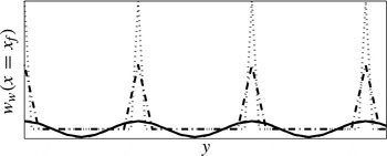
Suction and blowing are generated using two simple forcing models that are illustrated in figure 2 and characterized by the Fourier amplitudes:
 $$\begin{eqnarray}\text{I}\qquad w_{w,1}=c\quad \text{and}\quad w_{w,k}=0\quad \forall k\neq 1\end{eqnarray}$$
and
 $$\begin{eqnarray}\hspace{-55.20007pt}\text{II}\hspace{51.60004pt}w_{w,k}=c\quad \forall k.\end{eqnarray}$$
Scheme
 $\text{I}$
(solid and dashed lines, respectively, correspond to
 $N_{y}=4$
and 8 in figure 2) represents a periodic suction and blowing strip, where the sign of
 $c$
has no effect on the response of the cross-flow disturbance. Only the primary mode is initially excited, but through the processes of nonlinear interaction the growth of the higher-order harmonics is stimulated. All modes are forced equally by method
 $\text{II}$
(chain and dotted lines denote cases
 $N_{y}=4$
and 8 in figure 2), which in the physical plane approximately represents a band of small point-like periodic holes prescribed with either wall suction (negative
 $c$
) or blowing only (positive
 $c$
). As the value of
 $N_{y}\rightarrow \infty$
, the physical shape of the wall forcing will tend towards a Dirac-delta type function along the spanwise direction. Obviously, for finite
 $N_{y}$
, there will then be some inconsistencies between the disturbance amplitudes of solutions for different
 $N_{y}$
(which we will investigate further in subsequent sections). The size of the amplitude
 $c$
then imposes conditions on the receptivity analysis. For relatively small forcing amplitudes, the disturbance will remain linear for the early stages of the flow development. However, as the magnitude of
 $c$
increases, the effects of nonlinearity will become significant and affect both the initial size of the disturbance and the downstream development of the flow system.
Physical spanwise shape of wall forcing at
 $x=x_{f}$
. Method
 $\text{I}$
represented as solid
 $(Y_{N}=4)$
and dashed lines (8), while chain (4) and dotted (8) correspond to method
 $\text{II}$
with blowing
 $c$
positive.

Although the two wall schemes are crude representations of wall suction and blowing, and possibly physically unrealistic, they provide a simple means of testing the vorticity formulation and analysing the receptivity and development of cross-flow disturbances to varying forms of forcing. Implementation of more complex and physically realistic suction holes can then be modelled (on Spalart Reference Spalart, Arnal and Michel1990, Reference Spalart, So, Speziale and Launder1993) by modifying the relative sizes of the Fourier harmonics
 $w_{w,k}$
.
The no-slip condition (2.15) is included in the vorticity formulation by deriving two integral constraints for the principal vorticity variables
 $\{{\it\omega}_{x},{\it\omega}_{y}\}$
. This is achieved by rearranging the secondary variable definitions (2.12) for
 $u~(\equiv 0)$
and
 $v~(\equiv 0)$
as
 $$\begin{eqnarray}\int _{0}^{\infty }{\it\omega}_{x}\,\text{d}z=\int _{0}^{\infty }\frac{\partial w}{\partial x}\,\text{d}z\end{eqnarray}$$
and
 $$\begin{eqnarray}\int _{0}^{\infty }{\it\omega}_{y}\,\text{d}z=\int _{0}^{\infty }\frac{\partial w}{\partial y}\,\text{d}z.\end{eqnarray}$$
These two integral constraints replace the no-slip conditions (2.15a,b
) along the
 $x$
and
 $y$
directions. When coupled with the wall-normal
 $z$
condition (2.15c
), they provide the necessary set of boundary wall constraints on the above system of governing equations. Null conditions are imposed on perturbations at the upstream boundary, whilst at the opposite end of the spatial domain a wave-like condition is implemented that allows disturbances to propagate through the computational box without causing spurious reflection effects. Boundary conditions in the far-field limit are imposed on disturbance fields by ensuring that the three principal perturbation fields
 $\{{\it\omega}_{x},{\it\omega}_{y},w\}$
tend to zero as
 $z\rightarrow \infty$
(further details are included in Davies & Carpenter (Reference Davies and Carpenter2001)).
3. Numerical methods
3.1. Discretization
The numerical methods adopted for the discretization of the vorticity formulation are described as follows. Chordwise derivatives are represented using a fourth-order centred compact finite difference approximation, while a Fourier expansion (outlined above in § 2.2) is implemented along the spanwise direction. Along the wall-normal axis, a change in variable is implemented,
 $$\begin{eqnarray}{\it\xi}=\frac{L}{L+z},\end{eqnarray}$$
to map points from the semi-infinite physical plane
 $z\in [0,\infty )$
onto a finite computational box
 ${\it\xi}\in (0,1]$
. The mapping parameter
 $L=4$
prescribes the distribution of points along the wall-normal direction and was carefully chosen to ensure that the resolution of the disturbance structure (cross-flow and possible secondary instabilities) within and about the edge of the boundary layer is accurately resolved. Disturbances are then expanded in terms of Chebyshev polynomials
 $$\begin{eqnarray}q_{k}(x,z,t)=\mathop{\sum }_{j=1}^{N_{z}}q_{k,j}(x,t)T_{j}({\it\xi}),\end{eqnarray}$$
where
 $T_{j}$
is the
 $j$
th Chebyshev polynomial. Here
 $N_{z}$
is the order of the series truncation, and
 $j$
is an odd and even integer for the principal and secondary variables, respectively. (Subscript
 $k$
refers to the value of the harmonic in the Fourier series.) The system of governing equations (2.11) is then integrated twice with respect to the mapped variable
 ${\it\xi}$
, generating a simple set of banded matrix representations for the wall-normal variation. Finally, the time marching is treated using a combination of a predictor–corrector scheme and semi-implicit methods.
3.2. Computational parameter settings
Steady periodic cross-flow instability was generated by carefully selecting the following discretization parameters:
-
(i) number of wall-normal Chebyshev polynomials
 $N_{z}$
;
-
(ii) time step
${\rm\Delta}t$
; -
(iii) chord grid step
${\rm\Delta}x$
; -
(iv) chord domain size
$N_{x}$
; and -
(v) number of spanwise Fourier modes
$N_{y}$
.


As our investigation concerns the initial response of disturbances to periodic forcing, the above parameters were not constrained by the need to fully capture small-scale structures that could evolve following the development of nonlinear flow characteristics. Thus, well-resolved and numerically stable results (up to the chord location at which small-scale effects first appear) were successfully obtained by prescribing step sizes
 ${\rm\Delta}t=0.01$
and
 ${\rm\Delta}x=0.5$
. Further, it was deemed sufficient to set the number of Chebyshev polynomials
 $N_{z}=48$
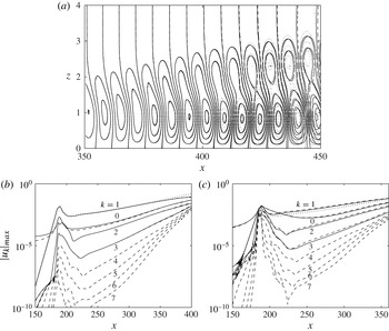
. Figure 3(a) illustrates the effectiveness of this parameter selection by comparing contours of the chordwise primary Fourier harmonic
 $u_{1}$
in the
 $(x,z)$
plane, which were established using the forcing method
 $\text{I}$
. The suction and blowing forcing was prescribed a zero frequency (
 ${\it\omega}=0$
), so that stationary cross-flow instabilities could develop, while the spanwise wavenumber
 ${\it\beta}=0.4$
and the Reynolds number
 $\mathit{Re}=500$
. The Gaussian distribution along the chord direction was centred about the position
 $x_{f}=186$
with an amplitude
 $c=0.01$
. The disturbance evolution is depicted over a short chordwise region, upstream of the onset of full nonlinear flow development. Solid lines display contours of the solution generated using the above parameter settings, while the dashed and dotted lines, respectively, denote solutions for the settings
 $\{{\rm\Delta}x,N_{z}\}=\{0.25,48\}$
and
 $\{0.5,64\}$
. All three sets of contour lines are indistinguishable up to the chordwise location
 $x=400$
, which, as we will observe in the subsequent discussion on receptivity, is downstream of the region of interest for this particular problem.
(a) Contours of the primary
 $u_{1}$
velocity Fourier harmonic for
 $\{{\rm\Delta}x,N_{z}\}=\{0.5,48\}$
(solid),
 $\{0.25,48\}$
(dashed) and
 $\{0.5,64\}$
(dotted). (b,c) Maximum amplitudes of the
 $N_{y}$
Fourier
 $u_{k}$
velocity fields for forcing methods (a)
 $\text{I}$
and (b)
 $\text{II}$
and amplitude of forcing
 $c=0.01$
. The Reynolds number
 $\mathit{Re}=500$
, spanwise wavenumber
 ${\it\beta}=0.4$
and centre of forcing
 $x_{f}=186$
. Solid lines indicate results generated using
 $N_{y}=4$
and dashed correspond to
 $N_{y}=8$
modes. (Dotted lines illustrate the linear-only results.)

The length of the chordwise domain was varied inversely proportional with the initial amplitude
 $c$
of the suction and/or blowing forcing. This ensured that disturbances of varying initial magnitude had sufficient chord length to develop. For the largest values of
 $c~({\sim}0.05)$
considered, the size of
 $N_{x}$
was limited to approximately
 $400{\it\delta}$
chord units beyond the forcing location
 $x_{f}$
, which was increased to
 $800{\it\delta}$
chord units for the smallest values of
 $c$
.
The final parameter necessary to generate successful and reliable nonlinear simulation results was the number of spanwise Fourier modes
 $N_{y}$
. Figure 3 also compares the maximum amplitudes of the Fourier
 $u_{k}$
velocity perturbations for
 $N_{y}=4$
(solid lines) and 8 (dashed) modes. Linear-only results are included and plotted using dotted lines for the purposes of comparing with the solutions of the nonlinear investigation. The flow specifications are as given above
 $\{{\it\omega},{\it\beta},\mathit{Re}\}=\{0,0.4,500\}$
for
 $\{x_{f},c\}=\{186,0.01\}$
. Steady disturbance amplitudes generated by method
 $\text{I}$
are depicted in figure 3(b), while figure 3(c) illustrates results driven by forcing scheme
 $\text{II}$
. Disturbances excited by
 $\text{I}$
for
 $N_{z}=4$
and 8 exhibit very minor variations that are barely noticeable on the given plot resolution. The two primary Fourier velocity components,
 $|u_{1}|_{max}$
, are identical over the chord length considered, and deviations from the linear result only emerge for
 $x>300$
.
Results generated using the second forcing method do not display such consistent behaviour, as there are relatively large differences between the two nonlinear and linear-only simulation results that appear almost immediately about the origin of forcing. There are also small discrepancies between the magnitudes of the two nonlinear calculations. Although these differences are marginal, they may be augmented as the amplitude
 $c$
of the initial forcing is increased to larger values. This behaviour is to be expected for method
 $\text{II}$
, as it is clearly illustrated in figure 2 that the physical representation of the point-like forcing can vary quite significantly for variable
 $N_{y}$
. Further nonlinear simulations were generated for larger
 $N_{y}$
Fourier modes, with results (discussed in subsequent sections regarding receptivity and nonlinear flow development) suggesting that additional harmonics have a relatively small effect on the size and evolution of the disturbance.
For the greater part of this investigation, it was decided that
 $N_{y}=4$
Fourier modes would be sufficient to study the general effects of nonlinearity on the receptivity and development of cross-flow. The primary reason behind the choice of
 $N_{y}$
was to save on both computational resources and time expenditure. Further it was suggested by Malik et al. (Reference Malik, Li and Chang1994) that the nonlinear characteristics of the cross-flow vortex could be modelled successfully using only the primary Fourier mode and its zeroth- and second-order harmonics. Although computations generated by method
 $\text{II}$
would inevitably vary for additional Fourier harmonics (as the physical representations of the wall forcing are different for variable
 $N_{y}$
), differences in disturbance amplitude and flow characteristics were relatively minimal, even for relatively large initial forcing sizes
 $c$
. Further discussion of the effect of increasing
 $N_{y}$
is included below, with results documented later in tables 1 and 2.
4. Disturbance definitions
In parabolized stability equation (PSE) analysis, linear cross-flow disturbances are assumed to take the form
 $$\begin{eqnarray}q(\boldsymbol{x},t)=A_{c}\tilde{q}(x,z)\exp \left\{\int _{x_{0}}^{x}{\it\alpha}(x^{\prime })\,\text{d}x^{\prime }+\text{i}({\it\beta}y-{\it\omega}t)\right\},\end{eqnarray}$$
where
 ${\it\alpha}$
is the chord wavenumber of the perturbation and
 $x_{0}$
corresponds to the location for neutral stability. Here
 $\tilde{q}$
is a shape function that varies slowly along the chord direction and is normalized about
 $x_{0}$
. The magnitude of the disturbance is represented by the real constant
 $A_{c}$
, which is described herein as the receptivity amplitude, for subscript
 $c$
the size of the initial forcing. For a linear-only analysis, the magnitude of
 $A_{c}$
is directly proportional to the size of
 $c$
as
 $$\begin{eqnarray}A_{c}=cA_{1},\end{eqnarray}$$
where
 $A_{1}$
is the amplitude of a cross-flow disturbance associated with
 $c=1$
. For the current investigation, it is convenient to assume that linear disturbances are also of the form (4.1), as it provides an effective means of extracting the wavenumber, growth rate and disturbance amplitude from the vorticity formulation computations.
4.1. Receptivity amplitude
By neglecting the slow chordwise variation of the shape function, setting
 $\tilde{q}(x,z)\approx \tilde{q}(z)$
, the definition for linear cross-flow can be simplified to the form
 $$\begin{eqnarray}q(\boldsymbol{x},t)=A_{c}\tilde{q}(z)\exp \left\{\int _{x_{0}}^{x}{\it\alpha}(x^{\prime })\text{d}x^{\prime }+\text{i}({\it\beta}y-{\it\omega}t)\right\},\end{eqnarray}$$
where we assume
 $|\tilde{q}|=1$
. Further, introducing a normalization factor, (2.8), and replacing the function
 $q$
with the primary Fourier chordwise perturbation field
 $u_{1}$
, we set
 $$\begin{eqnarray}M(x)=\max _{z}|u_{1}(x,z)|\,\frac{\mathit{Re}}{x}.\end{eqnarray}$$
A definition for the absolute value of the receptivity amplitude is then given as
 $$\begin{eqnarray}A_{c}=\frac{\displaystyle M(x)\frac{x}{\mathit{Re}}}{\displaystyle \left|\exp \left\{\int _{x_{0}}^{x}{\it\alpha}(x)\text{d}x\right\}\right|}.\end{eqnarray}$$
For a prescribed set of initial flow conditions,
 $\{{\it\omega},{\it\beta},\mathit{Re}\}$
, the exponential denominator is a fixed
 $x$
-dependent function that is not related to the choice of wall forcing. Thus, once the field
 $u_{1}$
is generated, the receptivity amplitude
 $A_{c}$
of the disturbance can be calculated. Though this expression is only applicable to linear cross-flow disturbances, we will also apply it to solutions of the nonlinear investigation, as it provides a means of comparing the two sets of results.
4.2. Saturation
The location at which the growth rate of the nonlinear disturbance first differs significantly from that given by the linear calculation is known as saturation. The interaction of the primary mode with the higher-order harmonics has become sufficiently large to impact on the disturbance evolution and the growth of the system. In an attempt to quantify nonlinear saturation, we define
 $$\begin{eqnarray}K_{\ast }(x)=\frac{M_{x}}{M},\end{eqnarray}$$
where the subscript
 $x$
refers to the chordwise derivative, while the subscript for
 $K$
is either
 $L$
for linear analysis or
 $NL$
for the corresponding nonlinear theory computations. The appearance of nonlinear saturation is then defined here as satisfying the expression
 $$\begin{eqnarray}F(x)\equiv \bigg|\frac{K_{NL}-K_{L}}{K_{L}}\bigg|\times 100\,\%>1\,\%,\end{eqnarray}$$
which was decided upon (following the analysis given in subsequent sections) as being a sufficiently large percentage difference to delineate between the linear and nonlinear results. Further, it was assumed that the linear disturbance function
 $K_{L}$
is non-zero and at the very least represents a convectively growing disturbance.
4.3. Stationary point
Finally, we introduce a definition that characterizes the chordwise location at which the absolute value of
 $M$
first attains a stationary point or peak value,
 $$\begin{eqnarray}M_{x}=K_{NL}=0\quad \text{and}\quad F(x)=100\,\%,\end{eqnarray}$$
which coincides with
 $M$
typically having a magnitude of approximately one-tenth of the spanwise free-stream velocity
 $V_{\infty }$
. Further, this location approximately coincides with the appearance of small-scale structures that arise with the emergence of nonlinear flow development.
5. Results
5.1. Disturbance development and growth
A steady stationary cross-flow disturbance was generated for approximately the strongest growing spanwise wavenumber
 ${\it\beta}=0.4$
, while the Reynolds number of the flow,
 $\mathit{Re}=500$
, is chosen, as it is smaller than the critical value for the attachment-line instability
 $(\mathit{Re}\sim 583)$
and allows easier comparison with solutions of earlier investigations (Malik et al.
Reference Malik, Li and Chang1994). Forcing scheme
 $\text{I}$
was centred about the chordwise location
 $x_{f}=186$
with amplitude
 $c=0.01$
. The periodic suction and blowing strip was then switched on at time
 $t=0$
, triggering the excitation of disturbances within the boundary layer. Downstream of the forcing a cross-flow instability evolves along the chordwise direction.
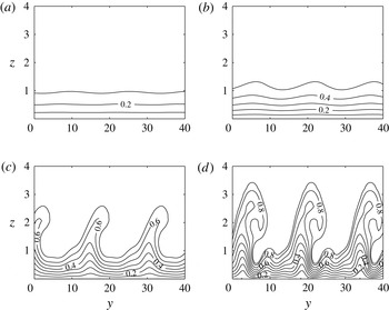
Figure 4 depicts cross-sectional cuts of the total
 $U$
velocity in the
 $(y,z)$
plane, plotted using labelled line contours at four successive positions along the chordwise direction:
 $x=200$
, 300, 400 and 450. The flow dynamics is plotted over two spanwise wavelengths, where the
 $z$
axis is stretched for visualization purposes. Contours are plotted from a value of 0 at the wall through to a maximum magnitude of approximately 0.9 in the far field. Cross-flow vortices are observed to evolve into the shapes described by Malik et al. (Reference Malik, Li and Chang1994) as half-mushroom structures. About
 $x=200$
the boundary layer thickness remains relatively constant along the length of the spanwise direction, as there are only small variations in the total velocity. However, at larger chord positions, the nonlinear effects emerge and the disturbance rolls into vortices, creating regions of low and high velocity. This in turn results in significant variations in the boundary layer thickness along the span. The evolution of the cross-flow vortex is comparable with that described by Malik et al. (Reference Malik, Li and Chang1994), even though only four spanwise Fourier modes are used herein to generate the disturbance.
Total chordwise velocity in the
 $(y,z)$
plane at
 $x=200$
, 300, 400 and 450, for
 ${\it\beta}=0.4$
and
 $\mathit{Re}=500$
.

(a) Disturbance growth rate for
 ${\it\beta}=0.4$
and
 $\mathit{Re}=500$
. Nonlinear primary mode with
 $c=0.03$
(solid line), 0.01 (dashed) and 0.001 (chain). The dotted curve corresponds to a linear-only disturbance. (b) Saturation prediction for the disturbances given in (a) with the formula based on that defined in (4.6b
).

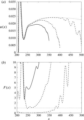
Figure 5(a) displays the growth rates of several linear and nonlinear disturbances calculated using the formula
 $$\begin{eqnarray}{\it\alpha}=\frac{1}{u_{1}}\frac{\partial u_{1}}{\partial x},\end{eqnarray}$$
where
 $u_{1}$
is the primary Fourier velocity component in the chordwise direction. The dotted line depicts the growth rate of the linear-only simulation, while the solid, dashed and chain lines represent the growth rates of the nonlinear primary mode, where the initial forcing
 $c=0.03$
, 0.01 and 0.001, respectively. In all four cases the periodic suction and blowing strip is centred about
 $x_{f}=186$
. In the chord region immediately downstream of the wall forcing, a short transient stage is observed, which is attributed to several perturbations initially competing to influence the response of the flow. However, the stationary cross-flow disturbance is eventually observed and the growth rates follow a set path. The linear growth rate behaves in a manner consistent with the observations of earlier studies on non-parallel linear effects. The growth rate attains a maximum value of approximately 0.25 near
 $x=350$
and slowly decreases thereafter. The development of the three nonlinear growth rates also follows a similar evolutionary path. However, as
 $c$
increases, the growth rate is found to saturate and deviate from the linear solution at varying chord locations. This is observed about the chord positions
 $x=250$
and 370 for the respective forcing amplitudes
 $c=0.01$
(dashed) and 0.001 (chain). These chord locations are also consistent with the calculations of the function
 $F$
, (4.6b
), displayed here in figure 5(b). Line types match those given for the above nonlinear solutions, while the horizontal dotted line now represents the suggested
 $F=1\,\%$
difference for the onset of nonlinear saturation. For the largest forcing amplitude,
 $c=0.03$
, significant differences between the linear and nonlinear growth rates appear directly about the centre of excitation with a minimum value for
 $F\approx 3\,\%$
. This would suggest that this represents a rather large-magnitude suction and blowing wall forcing. Thus, for greater initial forcing amplitudes, the linear stages of the disturbance development may be bypassed altogether.
5.2. Absolute perturbation velocity
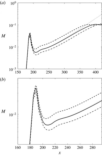
Figure 6 displays the maximum amplitude of the primary Fourier component of the
 $\bar{u}$
velocity against the chordwise
 $x$
direction, where (4.4) for
 $M$
has been utilized to simplify notation and illustrate solutions. The first plot shows results over an extended chord range, from upstream of the periodic forcing through to the location at which the disturbance first attains a stationary or peak point (as outlined in § 4.3). The second illustration presents results centred about the location of the periodic wall forcing. A semi-logarithmic scaling has been applied along the vertical axis to assist visualization and interpretation.
Maximum amplitudes
 $M$
for forcing schemes
 $\text{I}_{c=0.01}$
(solid),
 $\text{II}_{c=0.01}$
(dashed) and
 $\text{II}_{c=-0.01}$
(chain). The Reynolds number of the flow
 $\mathit{Re}=500$
, the spanwise wavenumber
 ${\it\beta}=0.4$
and centre of forcing
 $x_{f}=186$
. The dotted line represents the linear-only solution. (a) Extended chord range. (b) Localized about the centre of forcing.

The solid line depicts the disturbance solution established by forcing method
 $\text{I}$
for
 $c=0.01$
, where only the primary disturbance is excited. However, through the nonlinear processes the higher-order harmonics are generated and forced to grow proportionally with the primary mode. The nonlinear solution exhibits very small variations to the response of the linear computation (drawn using a dotted line). Comparing the perturbation development over an elongated chordwise frame (figure 6
a) would suggest that significant variations in magnitude appear only for
 $x>300$
. Indeed, the localized view of the perturbation in figure 6(b) indicates that the amplitude change about the wall forcing is relatively insignificant. This suggests that, in this instance, the nonlinear effects have very little impact on the receptivity of the disturbance and only appear through the modal interaction of the downstream development of the cross-flow vortex.
Dashed and chain lines depict simulation results driven by scheme
 $\text{II}$
where
 $c=0.01$
(blowing only) and
 $c=-0.01$
(suction), respectively. In these particular cases, all Fourier modes are now excited equally, but the higher-order harmonics are quickly forced to grow relative to the primary perturbation. The amplitude of the primary velocity component seeded using the wall forcing method
 $\text{II}$
displays a considerable variation from the linear-only simulation, both about the origin of the forcing and during the downstream development of the disturbance. Blowing increases the size of the disturbance, whilst suction shows a comparable reduction in the perturbation magnitude. Hence, the effects of nonlinearity are now very relevant to the receptivity process, as well as in the cross-flow evolution. These observations agree with the original findings of Choudhari & Duck (Reference Choudhari, Duck, Duck and Hall1996), who first noticed that the onset of nonlinearity could initially emerge in the receptivity stages of the flow development, very much before the subsequent appearance of nonlinear processes in the cross-flow disturbance.
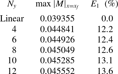
The effect of nonlinearity on the receptivity at the point of forcing
 $x_{f}$
is presented in table 1. The relative amplitudes of the primary mode
 $u_{1}$
are compared for varying Fourier harmonics
 $N_{y}$
, where results correspond to those disturbances generated using the blowing only forcing (method
 $\text{II}$
) for
 $c=0.01$
. Nonlinearity has increased the relative size of the perturbation about
 $x_{f}$
, but the percentage difference between the
 $N_{y}=4$
and 12 mode cases is very small, suggesting that our earlier assumption of four spanwise modes may be adequate for investigating cross-flow receptivity. Nevertheless, nonlinearity has had an effect on the local receptivity and size of the disturbance about the centre of wall forcing. However, in subsequent analysis we will observe that nonlinearity has an even greater impact on the effective receptivity amplitude of the developing cross-flow instability.
Comparing maximum amplitudes of the primary Fourier harmonic
 $u_{1}$
at the origin of forcing
 $x_{f}$
for disturbances with mode numbers
 $N_{y}=4,6,\dots ,12$
. Disturbances are generated using forcing scheme
 $\text{II}$
and
 $c=0.01$
. The parameter
 $E_{1}$
specifies the relative differences between the linear and nonlinear solutions.

The absolute maxima of the three disturbances attain a stationary point or peak magnitude about a value of 0.1, near the chord locations
 $x=370$
, 390 and 410 for forcing schemes
 $\text{II}_{c=0.01},\text{I}_{c=0.01}$
and
 $\text{II}_{c=-0.01}$
, respectively. Downstream of the stationary point, the maximum value of the primary mode is found to fluctuate about this amplitude. Small-scale structures are then observed to develop, but owing to the prescribed discretization (discussed earlier) are not captured to any degree of certainty. However, as the current investigation only concerns the effects of nonlinearity on receptivity and the early stages of disturbance evolution, any resolution errors beyond this stationary point can be safely ignored.
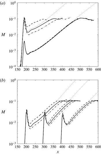
Additional plots of maximum disturbance amplitudes
 $M$
are presented in figure 7. The line types are the same as those given in figure 6. The first illustration (figure 7
a) depicts the effect of varying the forcing amplitude
 $c$
on the receptivity of the disturbance. Two forcing amplitudes are considered:
 $c=0.03$
in the upper half of the plot and
 $c=0.001$
in the lower half. There are no discernible differences between the perturbation amplitudes generated using the smaller forcing (at least for
 $x<400$
). However, those disturbances excited by the larger forcing amplitude are observed to display significant deviations from the linear-only response. This also includes the cross-flow disturbance established by wall forcing method
 $\text{I}$
, which now displays distinct variations in magnitude. Further, the size of
 $M$
, for the suction and blowing strip and blowing-only forcing, is greater about the centre of wall excitation than the amplitude observed downstream at the stationary point. The nonlinear effects have greatly influenced both the form of the local wall forcing and the magnitude of the developing disturbance. These observations agree with the earlier analysis on the system growth and the onset of saturation for the disturbances generated with initial amplitude
 $c=0.03$
. This would then suggest that these particular cases represent rather strong and probably physically unrealistic suction and blowing amplitude distributions.
Maximum amplitudes
 $M$
, where solid lines depict results due to forcing
 $\text{I}$
, dashed forcing
 $\text{II}_{\text{b}}$
, chain forcing
 $\text{II}_{\text{s}}$
and dotted the linear-only solution. The Reynolds number
 $\mathit{Re}=500$
and the spanwise wavenumber
 ${\it\beta}=0.4$
. (a) Centre of excitation
 $x_{f}=186$
and forcing amplitude
 $c=0.03$
(upper lines) and
 $c=0.001$
(lower lines). (b) Forcing amplitude
 $c=0.01$
and centre of excitation
 $x_{f}=200$
, 300 and 400.

The chord centre of the periodic forcing is varied in figure 7(b) to illustrate the effect of the disturbance distribution on the boundary layer receptivity. Again, the line types correspond to those forcing methods described above, where
 $c=\pm 0.01$
and
 $x_{f}=200$
, 300 and 400. The general receptivity characteristics at each selected chord location are again similar to that described above. Method
 $\text{I}$
has a marginal effect on the initial amplitude of the perturbation, whilst blowing and suction driven by forcing scheme
 $\text{II}$
again significantly augments and reduces the receptivity amplitude of the disturbance. As the centre of forcing
 $x_{f}$
passes downstream along the chord direction, the initial amplitude of the perturbation decreases and the location of the so-called downstream stationary point increases. This behaviour may be expected, as it is well known that the largest linear receptivity amplitudes are observed about neutrally stable conditions for cross-flow (
 $x_{0}\sim 186$
for stationary disturbances (Streett Reference Streett1998; Mughal Reference Mughal2012)). Hence, in figure 7(b), the effect of nonlinearity is greatest at
 $x_{f}=200$
, and as
 $x_{f}$
is increased to larger chord positions the nonlinear effects on the receptivity amplitude diminish and the gap between the dashed (blowing) and dotted lines (suction) reduces.


5.3. Amplitudes
The formula for the amplitude
 $A_{c}$
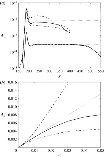
of the cross-flow instability, (4.5), is applied to both the linear and nonlinear perturbations in figure 7(a), which generates the plots shown in figure 8(a). Though the assumed PSE form of cross-flow is not particularly relevant or applicable to the nonlinear stages of the evolution process, it does provide a simple means of comparing the relative sizes of the primary mode of the linear and nonlinear solutions, especially in the chordwise region immediately downstream of the forcing. The two dotted lines depict the amplitudes given for the linear-only perturbations. Downstream of the periodic forcing, the linear receptivity amplitudes are relatively constant over the chord length considered and their respective values are related through the size of the initial forcing
 $c$
:
 $A_{1}=0.26$
,
 $A_{0.03}=0.0078$
and
 $A_{0.0001}=0.00026$
. The remaining line types depict the disturbance amplitudes given by the nonlinear solutions. The perturbations generated using the smaller initial forcing are almost identical over the chord length shown and only display significant variations from the linear result for
 $x>450$
. Downstream of this location, the amplitudes decrease rapidly, which agrees with the above observations, which are discussed and depicted in figure 7(a).
On the other hand, the amplitudes given for the larger initial forcing are shown to vary greatly. For instance, the perturbation established using the wall blowing method
 $\text{II}$
(dashed line) has a magnitude about
 $x=250$
that is approximately double that given by the corresponding linear disturbance, while the equivalent result for the suction-only forcing (chain line) is about half the size of the linear solution. As the cross-flow instability evolves and passes into the nonlinear development stages, the magnitude of the disturbance reduces and eventually all nonlinear amplitudes are smaller than the observed linear solution. This behaviour is due to the nonlinear interaction of the primary Fourier mode with its higher-order harmonics. Results for the larger initial forcing are cut off at
 $x=400$
, as this coincides with the onset of small-scale structures, which are beyond the resolution of the prescribed discretization.
Repeating the calculations given in figure 8(a) for
 $x_{f}=186$
and
 $c$
in the range 0.00001 to 0.05, the four lines or curves in figure 8(b) are generated that depict the relative sizes of
 $A_{c}$
against
 $c$
for solutions of the different forcing methods. The linear receptivity amplitudes, which are relatively constant over the chord length shown in figure 8(a), are given by the straight line
 $A_{c}=0.26c$
. The corresponding nonlinear amplitudes are selected at the chord location
 $x=250$
, which is chosen to give a meaningful representation of the receptivity and initial size of the disturbance. The results established by scheme
 $\text{II}$
are found to be reflected about the linear receptivity line, with suction (chain) having the expected stabilizing effect on receptivity amplitudes and blowing (dashed) destabilizing. The third nonlinear curve (method
 $\text{I}$
– solid) also shows a marked drop in the receptivity amplitude as
 $c$
increases, though it is not as exaggerated as that given for the suction-only case.
5.4. Stationary point and semi-logarithmic relationship
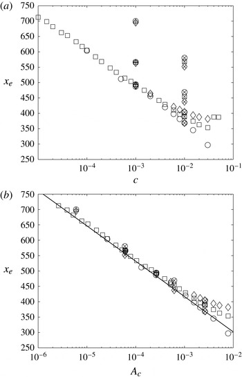
Figure 9 depicts the locations
 $x_{e}$
at which the flow parameter
 $M$
attains a stationary point against both the size of the initial forcing
 $c$
and the initial disturbance amplitude
 $A_{c}$
given by the linear-only analysis. A semi-logarithmic scaling has been used along the horizontal axis in both illustrations to aid visualization. The three nonlinear results are specified using the following symbols: ▫, method
 $\text{I}$
; ○, method
 $\text{II}$
, blowing; and ♢, method
 $\text{II}$
, suction. Open markers correspond to disturbances excited about
 $x_{f}=186$
, while symbols with a
 $\times$
and
 $+$
at the centre are associated with the wall forcing prescribed at
 $x_{f}=200$
, 300 and 400, with
 $c=0.01$
and 0.001, respectively. In figure 9(a) the calculations associated with the wall forcing centred about
 $x_{f}=186$
(open markers) are found to lie along the
 $(c,x_{e})$
diagonal. This is particularly true for those results computed for
 $c\leqslant 10^{-2}$
. However, for those disturbances excited at larger values of
 $x_{f}$
, the stationary points are shifted along the vertical axis, with the markers furthest from the diagonal representing the cases
 $x_{f}=400$
. The relative distances in
 $x_{e}$
between the results of cases
 $x_{f}=200$
and 300 are smaller than that found between
 $x_{f}=300$
and 400 because receptivity is strongest about the critical conditions for cross-flow instability
 $(x_{0}\sim 186)$
. The primary Fourier mode will attain the stationary point quicker for wall forcing located near this region. As the origin
 $x_{f}$
of the suction and blowing distribution is shifted downstream, the initial perturbation amplitude decreases and the location for the stationary point increases. The illustration then suggests that additional results for variable
 $x_{f}$
,
 $c$
and wall distributions
 $h(x)$
would also be scattered throughout the
 $(c,x_{e})$
plane.
The chord location at which the parameter
 $M$
attains a stationary point
 $x_{e}$
, plotted against (a) the amplitude of forcing
 $c$
and (b) the receptivity amplitude
 $A_{c}$
of the linear disturbance. Markers represent solutions given by the wall forcing methods: ▫, method
 $\text{I}$
; ○, method
 $\text{II}$
, blowing; and ♢, method
 $\text{II}$
, suction. Open markers correspond to disturbances excited about
 $x_{f}=186$
, while markers with a
 $\times$
and
 $+$
at the centre are associated with the wall forcing prescribed at
 $x_{f}=200$
, 300 and 400, with
 $c=0.01$
and 0.001, respectively. The solid line depicts the location at which the associated linear result attains a size of 0.1.

All positions
 $x_{e}$
are plotted against the linear receptivity amplitude
 $A_{c}$
in figure 9(b), where markers are as before. The solid line depicts the location at which the normalized linear calculation attains an amplitude of 0.1, which is consistent with the relative sizes of the nonlinear results at
 $x_{e}$
. Interestingly, all nonlinear results are located within a very small bandwidth about the solid line, including those generated using alternative forcing locations, initial amplitudes and methods. The plot suggests that, for a linear receptivity amplitude
 $A_{c}<10^{-3}$
, the chord position
 $x_{e}$
is located on the diagonal line given by the linear solution. As
 $A_{c}$
is raised to larger values, the range of
 $x_{e}$
increases quite significantly, with chord variations of the order of 100 for
 $A_{c}=10^{-2}$
. However, it may still be possible to give a crude approximation for the location for
 $x_{e}$
using a line of best fit or the linear-only calculation. A suitable fit for the linear result and nonlinear computations with
 $A_{c}\leqslant 10^{-3}$
is of the form
 $$\begin{eqnarray}A_{c}\equiv cA_{1}={\it\lambda}\,\text{e}^{{\it\gamma}x_{e}},\end{eqnarray}$$
where, after careful calculation, the constants
 ${\it\lambda}$
and
 ${\it\gamma}$
are respectively defined as 4.2 and
 $-0.02$
. For all problems considered herein, the amplitude results with the initial conditions
 $({\it\omega},{\it\beta},\mathit{Re})=(0,0.4,500)$
are located about this semi-logarithmic relationship.
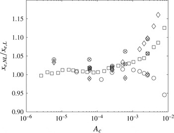
Figure 10 depicts the ratio of the stationary points for the nonlinear disturbances,
 $x_{e,NL}$
, and the associated linear result,
 $x_{e,L}$
. The ratio is plotted against the linear receptivity amplitude
 $A_{c}$
that is again drawn on a logarithmic axis. Markers are again as given in figure 9. For disturbances with receptivity amplitudes
 $A_{c}\leqslant 10^{-3}$
, the differences between the calculations of the linear and nonlinear solutions is at most 5 %. Thus, if the linear receptivity analysis indicates that the normalized disturbance magnitude attains a size of 0.1 about
 $x_{e,L}=500$
, then a nonlinear simulation would give
 $x_{e,NL}\in [475,525]$
. Hence, the simpler linear receptivity model may be used to estimate the location of disturbance processes in the more complex and time-expensive nonlinear analysis. In reference to the disturbance illustrated in figure 4 above, the position of the stationary point coincides with the cross-sectional velocity illustration that is depicted in 4(c), which is marginally upstream of the location at which the cross-flow instability has fully rolled into a vortex structure. Similar forms are observed about
 $x_{e}$
for other solutions, suggesting that the stationary point appears upstream of the location described by Malik et al. (Reference Malik, Li and Chang1994) and others as corresponding to full saturation.
Ratio of the location at which the nonlinear and linear
 $M$
computations attain a stationary point or amplitude 0.1. Markers are as given in figure 9.

In previous sections it was decided that
 $N_{y}=4$
Fourier modes was sufficient to investigate the receptivity and development of cross-flow disturbances in the swept Hiemenz boundary layer. This decision was primarily based on the computational and time cost of simulating many disturbances based on larger values of
 $N_{y}$
. However, as remarked upon above, disturbances to suction and blowing forcing scheme
 $\text{II}$
could possibly vary as
 $N_{y}$
is increased to larger values, causing the physical shape of forcing to asymptote towards a Dirac delta source. Hence, the results generated by forcing method
 $\text{II}$
may be inaccurate, particularly for large initial forcing amplitudes
 $c$
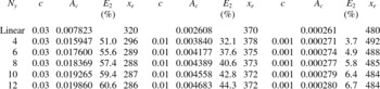
. Table 2 compares linear results with nonlinear calculations with varying orders of Fourier modes for the blowing-only forcing (positive
 $c$
). The initial receptivity amplitude of the disturbance,
 $A_{c}$
, the relative difference with the linear solution,
 $E_{2}$
, and the location at which the primary disturbance first attains a stationary point,
 $x_{e}$
, are documented. Following on from earlier observations, the chord location
 $x_{e}$
for the linear disturbance is given as the position at which the parameter
 $M$
attains a value of 0.1. Firstly, we note that the relative differences in the amplitude of the disturbance or effective receptivity are far greater than those percentage variations given for the local receptivity in table 1. For the smallest initial forcing,
 $c=0.001$
, the percentage differences
 $E_{2}$
for the
 $N_{y}=4$
and 12 mode cases are relatively similar, with values approximately given as
 $E_{2}=3.7\,\%$
and
 $6.7\,\%$
, respectively. Further, the variation in the location of the stationary point
 $x_{e}$
is very small, with linear predictions giving a very good estimate. This is also true of results given at the larger forcing,
 $c=0.03$
, with values for
 $x_{e}$
again consistent for all
 $N_{y}$
cases considered. Although the relative percentage variation,
 $E_{2}$
, is now much greater for all of the nonlinear simulations, the increase in receptivity amplitude from the
 $N_{y}=4$
to the 12 mode case is no more than 16 % (based on relative differences between these two particular solutions). Thus, as a first prediction of the effects of nonlinearity on the receptivity of the cross-flow development,
 $N_{y}=4$
Fourier modes appears to give a reasonable estimate of results even at very large initial suction and blowing forcing amplitudes.
Results of the initial receptivity amplitude
 $A_{c}$
, relative variation of the nonlinear amplitude with the matching linear result,
 $E_{2}=((A_{c,NL}-A_{c,L})/A_{c,NL})\times 100\,\%$
, and stationary point position
 $x_{e}$
, for
 $N_{y}=4,6,\dots ,12$
.

All of the results described above correspond to stationary-only disturbances with the Reynolds number of the flow
 $\mathit{Re}=500$
. Extending the above analysis to alternative values of
 $\mathit{Re}$
, and a travelling cross-flow disturbance, for
 ${\it\omega}=0.0375$
and dimensional frequency
 $f=20\times 10^{-6}~\text{Hz}$
, we can extract similar flow properties using the methods described above. The chordwise location for the onset of the cross-flow instability shifts upstream with decreasing Reynolds number, and is observed to emerge for stationary disturbances about
 $x_{0}=137$
, 160 and 186 for
 $\mathit{Re}=300$
, 400 and 500, respectively. The value of
 $M$
at the location at which the primary disturbance attains a stationary point,
 $x_{e}$
, is found to decrease with Reynolds number, with magnitudes typically approximately 0.09, 0.095 and 0.1 for the three Reynolds numbers considered. Semi-logarithmic plots are again constructed and depicted in figure 11 by plotting the location for
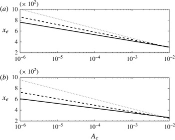
 $x_{e}$
against the linear receptivity amplitude
 $A_{c}$
. Clearly the value for
 $x_{e}$
increases to larger values as the Reynolds number decreases, meaning that transition will generally set in further downstream. Additionally, the investigated travelling wave disturbance is more unstable than the stationary mode, as the position of the stationary point (and onset of small-scale structures) appears earlier.
Chord location at which the primary disturbance attains a stationary point plotted against the linear receptivity amplitude
 $A_{c}$
: (a) stationary disturbances; (b) travelling wave for
 ${\it\omega}=0.0375$
. Dotted lines correspond to
 $\mathit{Re}=300$
, dashed
 $\mathit{Re}=400$
and solid
 $\mathit{Re}=500$
.

5.5. Receptivity of the physical perturbation
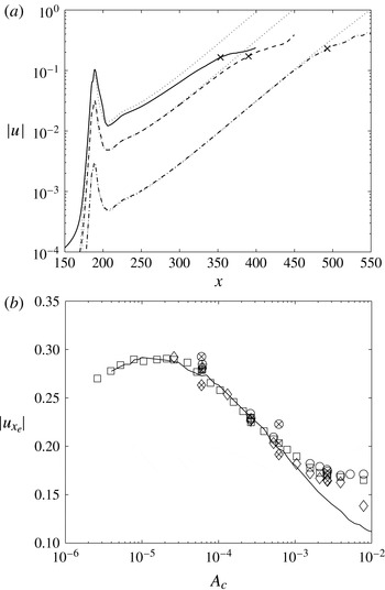
The analysis in the preceding sections documents the flow dynamics and receptivity characteristics of the primary Fourier velocity component. Initial receptivity amplitudes and the chord location at which the primary mode attains a stationary state are shown to be proportional on a linear semi-logarithmic mapping. However, from a physical perspective, it would be preferable to describe the flow properties of the real disturbance and its relationship (if any) to the receptivity amplitude. Figure 12(a) displays the disturbance response of the absolute value of three
 $u$
velocities as a function of
 $x$
. Solid, dashed and chain lines correspond to the nonlinear flow solutions excited by forcing scheme
 $\text{I}$
for the respective amplitudes
 $c=0.03$
, 0.01 and 0.001. The dotted lines depict the corresponding linear-only disturbance computations, while the three cross symbols specify the chord locations at which the associated primary disturbance
 $u_{1}$
first attains a stationary point
 $x_{e}$
. For these three illustrated cases, the position
 $x_{e}$
is observed when the absolute amplitude of the physical perturbation is
 $|u|=$
0.165, 0.17 and 0.23, respectively. (Note that the results have not been normalized on the factor
 $\mathit{Re}/x$
.)
(a) Absolute amplitude of the
 $u$
velocity perturbation against the chord direction
 $x$
. Nonlinear disturbances are excited about
 $x=186$
for initial forcing amplitudes
 $c=0.03$
(solid), 0.01 (dashed) and 0.001 (chain). (b) Magnitude of
 $u$
velocity component at
 $x_{e}$
plotted against the linear receptivity amplitude
 $A_{c}$
for all results given in figure 10.

Figure 12(b) displays the computed values of
 $|u|$
at
 $x=x_{e}$
for all results shown in figure 9. The marker specifications are as before, and a logarithmic scaling is implemented along the horizontal axis that again represents the linear receptivity amplitude
 $A_{c}$
. Behaviour similar to that depicted in figure 9(b) is again observed. The magnitude of the nonlinear
 $\bar{u}$
velocity perturbations is found to lie about the solid curve that represents the size of the linear
 $u$
velocity at the position
 $x_{e}$
. In particular, for
 $A_{c}\leqslant 10^{-3}$
, the results may be estimated by the curve given by the linear analysis that passes through all nonlinear results. Further, the absolute size of the disturbance
 $|u|$
, at the chord location
 $x_{e}$
, is observed to attain a maximum of 30 % of the free-stream velocity
 $V_{\infty }$
for a linear receptivity amplitude
 $A_{c}\sim 10^{-5}$
.
6. Final remarks
An investigation has been carried out on the effects of nonlinearity on the receptivity of cross-flow in the swept Hiemenz boundary layer. A nonlinear vorticity formulation has been developed, extending the scheme of Davies & Carpenter (Reference Davies and Carpenter2001) that was limited to linear disturbance development. Periodic forcing is prescribed in time and along the spanwise direction, using artificial suction and blowing strips or as bands of small holes. The effects of varying the origin and size of wall forcing are considered, as well as the effect of flow Reynolds number. Evolution of the cross-flow vortex is described and shown to exhibit flow characteristics consistent with that depicted in earlier investigations, even though only four spanwise Fourier modes are used to generate the nonlinear results. The analysis shows that solutions generated for larger modal numbers have a relatively small impact on both the local and effective receptivity of the cross-flow instability.
Suction and blowing distributed as periodic holes are shown to have a relatively large effect on the boundary layer receptivity. This is particularly true for those disturbances generated using large forcing magnitudes and centred near the chord location for critical cross-flow instability. The absolute maximum of the primary chordwise velocity perturbation, when normalized on
 $\mathit{Re}/x\equiv V_{\infty }/U_{\infty }$
, is observed to attain a stationary position for an amplitude near 0.1 and is shown to be linearly proportional (on a logarithmic scaling) with the initial receptivity amplitude given by the linear analysis. This is especially true of disturbances with values
 $A_{c}<10^{-3}$
and all wall forcing types considered. (Extensions to wall roughness may be possible by modifying the no-slip condition and deriving similar relationships for receptivity and stationary points.) This would suggest that some nonlinear flow dynamics of the cross-flow vortex development may be estimated directly from the linear receptivity analysis. In terms of the size of suction and blowing wall forcing, a disturbance with initial amplitude
 $A_{c}=10^{-3}$
that is generated by a Gaussian-shaped wall distribution about
 $x=186$
corresponds to an initial forcing magnitude of size
 $c=0.004$
or dimensionally
 $0.004V_{\infty }$
.
The logarithmic law relationship relating
 $x_{e}$
and
 $A_{c}$
is similar to the analysis based on the
 $n$
-factor method for transition. Assuming that
 $A_{c}$
is the initial size of the disturbance, then the amplitude at
 $x_{e}$
is given as
 $0.1x_{e}/\mathit{Re}$
, which gives the following formula for the
 $n$
-factor:
 $$\begin{eqnarray}n=\ln \biggl(\frac{x_{e}}{10A_{c}\mathit{Re}}\biggr).\end{eqnarray}$$
However, as
 $x_{e}$
is located upstream of the onset of full cross-flow saturation, this formula will slightly underestimate the predicted value of the
 $n$
-factor at transition.
Acknowledgements
We thank the referees for many helpful suggestions concerning the presentation and improvement of our results. This work was carried out with the support of EPSRC through LFC-UK: Development of Underpinning Technology for Laminar Flow Control.