It is an old saw that “networks matter” to both individual political decision making and macro political outcomes. While there are various conceptualizations and operationalizations of what “is” network, nearly all useful notions highlight the importance of communication through networks, regardless of whether one considers formal network structures (such as chains of command, committee structures and explicit communications networks such as social media) or less formal and more amorphous ones. In general, communication is a sequential process; some agents observe the actions and/or messages of others prior to making their own decisions. The strategic effects of network structure can be subtle and complicated when agents are aware of other agents’ abilities to observe prior decisions, and take this possibility into account when making their own decisions. And the vast heterogeneity of structures that might characterize even relatively small networks adds an additional layer of complexity to network analysis.
Network analysis has played a role in understanding various political phenomena, including legislator behavior,Footnote 1 judicial decision making,Footnote 2 public policy formationFootnote 3 and mass political behavior.Footnote 4 Unsurprisingly, the general development of social-scientific network analysis from both empirical and theoretical perspectives has attracted increasing interest as well.Footnote 5 Two of the main challenges confronted by network analysis are (1) the strategic effects of the network on the embedded agents’ behavior and (2) the aforementioned wide variety of possible network structures.
Scholars have acknowledged and tackled each of these challenges. In particular, Jackson (Reference Jackson2008) offers a very recent and comprehensive accounting of the state of the field in terms of both the basics of network theory and the theoretical underpinnings of strategic interactions in networks. In this article, we continue developing the theory of strategic interaction within networks (as opposed to the theory of their strategic formation) and focus on the effects of fine-grained details of network structure (that is, the network structure, per se, as opposed to convenient, but imperfect, summary statistics of its structure) on both individual strategic behavior and aggregate policy outcomes.
Our interest in this article is incentive compatibility within communication networks. That is, our primary focus is on what kinds of networks––in terms of (1) the preferences and decision-making powers of the agents in the network and (2) the structure of the network, and the positions of the various agents within the network––support the truthful communication of policy-relevant information between the agents. We adopt an abstract approach in this article: we do not utilize a specific application as a running example. Thus, before continuing to a more fine-grained discussion of our model, it is important to provide a motivatation for this focus in terms of political phenomena. In our view, incentive-compatible networks are more “stable” than networks that, for whatever reason, create an incentive for one or more agents to lie or obfuscate. After all, truthful communication (that is, larger numbers of agents being truthful with each other) will, ceteris paribus, support more accurate individual decision making in decentralized environments. Thus, on the margin, individuals should prefer to participate in truthful/incentive-compatible networks. This point suggests the distinct possibility of a selection effect at play when scholars and practitioners attempt to estimate the “effects” of various aspects of networks––for example, network structure, agents’ locations within a given structure or the diversity of agent preferences within the network––on (for example) individual and collective decision making. To the degree that this is true––which is beyond the scope of this article––the results reported here, and the logic upon which they are founded, are relevant to each of the topics listed earlier in which networks have been (and are) being studied. Starting from that point, we now discuss the specifics of our theoretical approach.
Small Networks
We focus in this article on (very) small networks. This focus is motivated by two seemingly contradictory realities. First, there are simply “too many” large network structures to analyze using the detailed, non-cooperative game theoretic techniques that we employ here. Second, small networks can in some sense be thought of as exhibiting “more extreme” variation in their structures. Specifically, while it is well known that changing a single link in any network can have surprisingly large effects, such sensitivity is almost tautological when considering small networks. These two realities (along with the fact that many big networks are really just networks of smaller networks) combine to suggest that understanding strategic decision making in small networks may provide sizable insight into such phenomena in larger networks.
Within small network settings, we examine decision making in what can be described as “distributed incomplete information environments.” Specifically, we suppose that each agent in the network has some private information about a policy-relevant variable—information that we presume is instrumentally valuable to every agent, though not necessarily equally valuable to all agents. Leaving the network aside for the moment, each player's private information can then be used when choosing his or her own individual (policy) decision.Footnote 6
The network structure comes into the picture by allowing some agents to observe other agents’ policy choices prior to making their own decisions. The network structure is assumed to be known to the agents, so that the possibility that other agents may use one's own policy decision in forming their individual policy choices can alter the incentive to truthfully set policy (that is, choose the player's most-preferred policy given his or her information).
Intuitively, the primary determinant of whether the network will induce such preferences is the degree to which the agents who might observe one's own policy decision prior to making their own have policy preferences that are (sufficiently) different from one's own. After all, if the individuals who will observe your choice have the same interests as you, the possibility of informing their decisions with your own amplifies the incentive to truthfully respond to one's own private information so as to convey this information to those making their decisions later. Thus in a nutshell, the most interesting results arise when there is preference divergence between the various agents.
Of course, preference divergence between actors within a network is an empirical regularity in many political environments (for example, consider the preference landscapes of most real-world legislatures, courts and electorates) and represents a key (and often fatal) challenge to achieving full information aggregation.Footnote 7 Small networks are a particularly important setting for the consideration of information aggregation: in many environments, the ex ante marginal social value of additional information is decreasing (that is, social ex ante payoff is an increasing, but concave, function of the number of “signals”).
With this motivation and context provided, we are now in a position to present our model of choice and signaling. We use this model to analyze the effects of network structure on information aggregation in groups with heterogeneous preferences. Our main theoretical innovation in this regard is that we allow for “credible” (or “non-cheap talk”) signaling in the sense that messages are conveyed through action choices that can have per se policy impacts. The basic theoretical framework is borrowed from Galeotti, Ghiglino and Squintani (Reference Galeotti, Ghiglino and Squintani2013).Footnote 8 As will become clear in the presentation of the model, this framework presumes that agents have “coarse” information, which makes the equilibrium analysis straightforward.Footnote 9
We present the basics of the model and then consider the canonical case of two agents. This analysis elucidates the moving parts of the theory and provides insights into the effects of the network on individual incentives. We then turn to the case of three-agent networks. This analysis highlights the importance of sequence in determining the possibility of information aggregation in equilibrium in this type of setting. In particular, it matters not only who observes your choice, but also who observes the choices of those who observe the choices of those who observe your choice.Footnote 10
After discussing the two- and three-agent network settings, we turn to consider some of the implications of the findings for both empirical work on networks and the design of incentive-compatible networks. From an empirical standpoint, our results highlight the importance of collecting and conditioning on rather fine-grained information when examining the impact of preferences, power and network structure on both individual and aggregate decision making. In particular, we provide an example that demonstrates the importance of the order of decision making in determining whether individual incentives are truthful. Relatedly, and from a design standpoint, we partially characterize a fundamental tension presented by the trade-off between (1) the potential informational efficiency of later decision makers utilizing earlier decision makers’ information and (2) the possibility that the knowledge that later decision makers are observing earlier decisions will undermine earlier decision makers’ incentives to be truthful when making their own policy decisions. We then offer a few concluding thoughts and suggestions for future research.
The Model
Let N denote a set of n individuals, X = R denote a policy space and Θ = [0,1] denote a state space. Each individual i∈N is initially (or formally) endowed with policy-making authority αI ≥ 0, which measures the degree of unilateral decision-making autonomy possessed by player i∈N, and the profile of these authorities is denoted by α = {αi}i ∈N. The state of nature, θ∈Θ, is determined according to a distribution characterized by cumulative distribution function F:[0,1]→[0,1]. Upon realization of θ according to F, each individual i∈N receives a conditionally independent (and private) signal si∈{0,1} according to the following probability mass function:
 $$ {\rm{Pr}}[{{s}_i}\, = \,x|\theta ]\, = \,\left\{ {\matrix{ {{\rm{1}}\,{\rm{ - }}\,\theta } & {{\rm{if}}\,\,x\, = \,0,} \cr \theta & {{\rm{if}}\,\,x\, = \,1. }}}\right. $$
Letting gi(·|si) denote the probability density function of i's posterior probability distribution function of θ, given si∈{0,1}, this belief is given by:
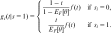 $${{g}_i}(t|s\, = \,{\rm{1}})\, = \,\left\{ {\matrix{ \displaystyle {\frac{{1\,{\rm{ - }}\,t}}{{1\,{\rm{ - }}\,{{E}_F}[\theta ]}}f(t)} & {{\rm{if}}\,\,{{s}_i}\, = \,0,} \cr { \displaystyle \frac{t}{{{{E}_F}[\theta ]}}f(t)} & {{\rm{if}}\,\,{{s}_i}\, = \,{\rm{1}. }}}}\right. $$
If F is the cumulative distribution function for the Uniform [0,1] distribution, then:
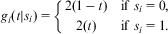 $$ {{g}_i}(t|{{s}_i})\, = \,\left\{ {\matrix{ {{\rm{2}}({\rm{1}}\,{\rm{ - }}\,t)} & {{\rm{if}}\,\,{{s}_i}\, = \,{\rm{0}},} \cr {{\rm{2}}(t)} & {{\rm{if}}\,\,{{s}_i}\, = \,{\rm{1}}.}}} \right. $$
Note that the uniform distribution is a useful baseline, as it maximizes the ex ante informativeness of each player's signal. In other words, this is the case in which information aggregation is most important to all players from an ex ante perspective.Footnote 11 Due to both this and the substantial analytical tractability that this assumption provides, we assume throughout this article that F is the uniform distribution. We are now in a position to define and discuss the individuals’ policy payoffs.
Payoffs
Each player i∈N chooses policy yi∈R; the vector of these decisions is denoted by y = (y 1,…,yn), and has a payoff function of the following form:
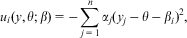 $$ {{u}_i}(y,\theta ;\beta )\, = \,{\rm{ - }}\mathop{\sum}\limits_{j\, = \,1}^n {{\alpha }_j}{{({{y}_j}\,{\rm{ - }}\,\theta \,{\rm{ - }}\,{{\beta }_i})}^{\rm{2}}}, $$
where βi∈R denotes the policy preference (or, perhaps, bias) of player i and β ≡ {βi}i ∈N denotes the profiles of all biases. We assume throughout that these biases are common knowledge to all of the players. Note that the autonomy of each player j factors into the payoffs of every player (including j) by determining the importance of j's decision. Thus, setting αj = 0 is equivalent to eliminating j's decision-making authority, but not necessarily the possibility that his or her choice of “policy” will be informative to other players who observe j's choice.
We pause for a moment to discuss the terming of αi as player i's “authority.” Our intention is to capture the idea that the decision of agent i “matters more” to all agents for larger values of αi. Of course, authority––like “power”––is a famously nebulous concept, and this conception is distinct from, for example, the notion of discretionary authority used in “delegation interval models,”Footnote 12 in which the measure of “authority” is the range of policies from which the agent in question can choose. For reasons of both focus and space, we are uninterested in the microstructure of policy making or authority: our interest is directed at the incentive to manipulate the beliefs of another decision maker. In this sense, the weight of that player's decision in one's own payoff function is essentially “all that matters.” Accordingly, we note that the term “authority” can be interpreted as merely a placeholder to refer to whatever empirical referent may more precisely describe whatever it is in a given context that makes one agent's decision matter more than another's. Of course, while our framework is general and “authority” is properly interpreted in generic terms, our framework does impose an important restriction: all agents assign identical weight to any given agent i's decision. One could generalize this, but we leave this extension for future work. We now proceed to define and describe the network structures at the heart of the article's analysis.
Networks
A network is a (directed) graph, G = (N, E), where N is the aforementioned set of n individuals and E is a set of M edges, E = {e 1,…,eM}, where e = (i, j) with i representing the “sender” of edge e and j representing the “receiver” of edge e. In other words, j observes the decision of i (yi) prior to choosing his or her own decision (yj). The network is common knowledge to all players.
In this article, we restrict attention to acyclic networks. This means that E contains no cycles: if e = (i, j)∈E is an edge in the network, there is no path of edges in E beginning with j and ending with i.Footnote 13 This assumption implies that when a player i observes another player j's decision, he or she knows that the observed decision is not conditioned in any way on i's own private information. Relaxing this assumption is possible but involves making additional assumptions about players’ abilities to revisit and revise their policy decision. Allowing revision greatly increases the complexity of strategic behavior. Eliminating revision and forcing choice at the first (agent-specific) available opportunity for each player is equivalent to presuming the network is acyclic. Accordingly, we simply assume that the network is acyclic and that each player makes a single and final choice at his or her first opportunity. Because we have assumed that N is finite and the network is acyclic, the set of edges implies an essentially unique game form in terms of the timing of decisions. In particular, fixing the set of edges, E, we denote the set of players whose decisions are directly observed by any given player i through E by σE(i).
With this notation in hand, we denote an instance of our setting by γ = (G, α, β, F), where G is the network (which also identifies the set of n individuals, N), and α and β represent the profiles of the individual's policy-making authorities (α) and biases (β),Footnote 14 and F is the cumulative distribution function of the state of nature, θ. To be clear, we assume throughout that the structure of the game (γ) is common knowledge among all of the individuals in N. We now turn to the discussion of policy decisions and preferences in this setting.
Policy and Preferences
One can distinguish between the two possible signals as failures (si = 0) and successes (si = 1). A success in this context can be thought of simply as a (coarse) indication that the state of nature is more than likely above its ex ante expected value and, conversely, a failure indicates that the state of nature is more than likely below its ex ante expected value.Footnote 15
Taking a decision-theoretic stance for a moment,Footnote 16 a player's posterior beliefs about θ after m trials and k successes (that is, k occurrences of s = 1 and m − k occurrences of s = 0) are characterized by a Beta (k+1, m − k+1) distribution, so that:
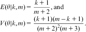 $$ \matrix{ E(\theta |k,m)\, = \displaystyle \,\frac{{k\, + \,{\rm{1}}}}{{m\, + \,{\rm{2}}}},{\rm{and}} \cr \ \ \ \ \ \ \ \ \ \ V(\theta |k,m)\, = \displaystyle \,\frac{{(k\, + \,1)(m\,{\rm{ - }}\,k\, + \,{\rm{1}})}}{{{{{(m\, + \,{\rm{2}})}}^{\rm{2}}} (m\, + \,{\rm{3}})}}. \cr} $$
Accordingly, the optimal policy choice for a policy maker, given (truthful) revelation of k successes and m − k failures, is:
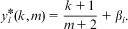 $$y_{i}^{\ast} (k,m)\, = \,\frac{{k\, + \,{\rm{1}}}}{{m\, + \,{\rm{2}}}}\, + \,{{\beta }_i}.$$
Equation 2 is used throughout our analysis. In words, a decision maker setting policy on his or her own should set it increasingly “higher” as the proportion of successes he or she is aware of increases. Furthermore, the individual decision maker's policy bias is reflected in his or her optimal policy decision simply as a linear shift equal to the bias: a positive bias (βI > 0) leads the player to choose a “higher than expected” policy ( $$$ y_{i}^{\ast} (k,m)\, \gt \,E(\theta |k,m) $$$
) and, conversely, a negative bias leads the player to choose a policy that is lower than expected.
Strategies and Beliefs
Before presenting the results, we first consider the formal definition of the game. In particular, the issue of belief formation is fundamental in this setting. Our equilibrium concept is perfect Bayesian equilibrium (PBE).
Information Sets
The set of information sets for player i∈N is denoted by  $$$ {{{\cal I}}_i} $$$
. In particular, for any network E, each player i∈N observes si as well as the decision yj for each player
 $$$ j \in {{\sigma }_E}(i) $$$
. Thus,
 $${{{\cal I}}_i}\, = \,\{ 0,1\} \,\times \,{{X}^{\left| {{{\sigma }_E}(i)} \right|}} .$$
Strategies
A (pure) strategy for player i∈N (xi) is simply a mapping from  $$$ {{{\cal I}}_i} $$$
to X:
 $$ {{x}_i}:{{{\cal I}}_i} \rightarrow R, $$
which describes the policy that player i chooses in each of his or her information sets.
Beliefs
In a PBE, players’ beliefs are correct on the equilibrium path of play. This consistency requirement is built into the calculations presented later in the text. The only tricky part of belief specification in these games involves off-the-path beliefs: namely, what should any player i∈N infer about the signals observed by another player j∈N when player j chooses a policy yj that is not sequentially rational, given the information structure of the game and player j's (commonly known) preference bias, βj.
For any player i∈N and network E, let μE(i) denote the maximum number of signals that i can infer, given E. This quantity can be defined as follows. For each i∈N, let AE(i) denote the “antecedent” players whose actions are observed by any player(s) whose actions are observed by any players whose actions are observed by … any player whose action is observed by i. Then,
 $$ {{\mu }_E}(i) = |{{A}_E}(i)| + {\rm{1}}. $$
Given the network E, a belief for player i at any information set  $$$ I \in {\cal I}(i) $$$
is essentially a probability distribution over {0,…,μE(i)}.Footnote 17 In a separating equilibrium, such a belief will be degenerate at any information set reached with positive probability (that is, on the equilibrium path of play). At all other information sets, however, the beliefs are essentially unrestricted.
A key point in defining beliefs in this framework is that, for each player i∈N, μE(i) is common knowledge to all players. Accordingly, and given the supposition that all players other than i and j are using pure strategies, player i need only infer something about what player j knows that player i does not. There is at least one such “thing,” namely the realization of j's signal, sj, but there may be more, depending on whether i can observe (directly or indirectly) all policy decisions that j had observed (again, directly or indirectly). Let δE(j,i) denote the set of players whose signals can be inferred by i only through j's policy choice, yj.Footnote 18 Then, letting ki denote the number of successes inferred or observed by i from his or her own signal and the observed choices (if any) by all players other than j, a deviation by j in terms of yj can affect i's beliefs only by altering them within the range  $$$ \{ {{k}_i}, \ldots, {{k}_i} + \left| {{{\delta }_E}(j,i)} \right|\} $$$
. Thus, the relevant beliefs of player i about the information that player j observes/infers that i can infer only from yj can be effectively represented by a probability distribution over {0,1,…,|δE(j,i)|}. Presuming that the other players are each playing separating strategies and given a policy choice yj by player j, this distribution for player i over this set for another player j is denoted by hi(·|yj).
Note that, as described above in Equation 2, for each value z∈{0,1,…,|δE(j,i)|}, there is a unique sequentially rational policy choice for player j,  $$$ y_{i}^{\ast} (z,|{{A}_E}(j)|) $$$
.Footnote 19 Because we are considering pure strategy PBE profiles, we need to consider out-of-equilibrium beliefs only up to the point that a single player deviates from his or her pure strategy.Footnote 20 Player i knows βj and βi: accordingly, we presume his or her off-the-equilibrium-path beliefs are essentially specified as follows.
Definition 1: For each distinct pair of players i,j∈N, let cij∈Z+ denote the number of successes commonly inferred by players i and j. Then player i's beliefs about j's information, given that all players other than j are using separating pure strategies, hi(zj|yj,cij), satisfy the following:
• if βj > βi:
 $$ \qquad \qquad \qquad \ \ {{h}_i}({{z}_j}|{{y}_j})\, = \,\left\{ {\matrix{ {\rm{1}} \hfill & {if\,{{z}_j} = \max \{ z \in \{ 0,1, \ldots, \left| {{{\delta }_E}(j,i)} \right|\} :y_{j}^{\ast} (z + {{c}_{ij}},{{\mu }_E}(j))\leq {{y}_j}\}, } \hfill \cr {\rm{0}} \hfill & {otherwise{\rm{,}}} \hfill}} \right $$
• and, if βj≤βi:
 $$ \qquad \qquad \qquad \ \ {{h}_i}({{z}_j}|{{y}_j})\, = \,\left\{ {\matrix{ {\rm{1}} \hfill & {if\,{{z}_j} = \min \{ z \in \{ {\rm{0}},{\rm{1}}, \ldots, \left| {{{\delta }_E}(j,i)} \right|\} :y_{j}^{\ast} (z\, + \,{{c}_{ij}},{{\mu }_E}(j))\geq {{y}_j}\}, } \hfill \cr {\rm{0}} \hfill & {otherwise{\rm{.}}} \hfill}} \right $$
The defined beliefs are simplest to understand in the baseline case in which player j observes only his or her signal, sj. When this is the case, there are two sequentially rational decisions for j:  $$$\frac{1}{3} $$$
+βj and
 $$$\frac{2}{3} $$$
+βj. Supposing that βj > βi, the beliefs defined in Definition 1 imply that i will infer that sj = 0 unless yj ≥
 $$$\frac{2}{3} $$$
+βj, in which case i infers that sj = 1.
These beliefs are designed to maximize the “costliness of manipulation” by player j of player i's beliefs subject to allowing player j to choose policies that are sequentially rational given his or her information when signaling truthfully to player i.Footnote 21 When β j > βi and i acts in a sequentially rational fashion when setting yi, there is never an incentive for j to manipulate i's beliefs such that i believes that sj = 0 when in fact sj = 1: j always prefers that i believes that j's signal is at least as high as it truly is.Footnote 22 Accordingly, the beliefs defined in Definition 1 require that j “go all the way” in his or her policy choice in order to manipulate i's beliefs in the direction that i knows is the only direction in which j has an incentive to manipulate i's beliefs.
Two Agents
Before continuing to the general model, we first consider the baseline case of exactly two players. Let N = {1,2}. In this case, there are two networks (up to symmetry): E = {}, representing independent (or “simultaneous”) policy making and E = {(1,2)}. The first network is unsurprisingly simple to analyze. Strict dominance implies that each of the two players should make his or her decision truthfully, as he or she can not affect the other player's decision in any case. We accordingly note this, set the empty network to the side and focus exclusively on the second network, E = {(1,2)}. This network represents a classic signaling game with Player 1 as the sender and Player 2 playing the role of the receiver, and establishes a baseline for the analysis in the following section. Throughout, we suppose that Player 2 is known to have observed m ≥ 0 trials and Player 1 has observed one trial.Footnote 23 As mentioned above, the network E = {(1,2)} is the foundation of a classic signaling game. If α 1 > 0, this signaling game is “costly” in the sense that the sender's message (that is, his or her policy choice) has direct payoff implications for the sender.
We allow Player 1 to have nontrivial decision-making authority (α 1 > 0). And—as in the pure signaling case analyzed above—in a separating equilibrium, Player 2 will use Player 1's policy decision to correctly infer Player 1's signal (s 1) and update his or her own policy decision (y 2) accordingly. When Player 1 has decision-making authority, α 1 > 0, his or her signal to Player 2 is conveyed through an action that has per se policy consequences. In order to keep the presentation succinct, presume that β 1 > β 2.
Note that, because δE(1,2) = {1}, Player 2's sequentially rational strategy as a function of his or her signal (s 2) and the policy chosen by Player 1 (y 1) given beliefs h 2 as described in Definition 1, is as follows:
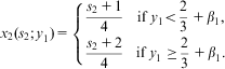 $$ {{x}_{\rm{2}}}({{s}_{\rm{2}}};{{y}_{\rm{1}}})\, = \,\left\{ {\matrix{ \displaystyle {\frac{{{{s}_{\rm{2}}}\, + \,{\rm{1}}}}{{\rm{4}}}} & { {\rm{if}}\,{{y}_{\rm{1}}} \lt \displaystyle \frac{2}{3}\, + \,{{\beta }_{\rm{1}}},} \cr { \displaystyle \frac{{{{s}_{\rm{2}}}\, + \,{\rm{2}}}}{{\rm{4}}}} & {{\rm{if}}\,{{y}_{\rm{1}}}\geq \displaystyle \frac{2}{3}\, + \,{{\beta }_{\rm{1}}}.}}} \right$$
Given the behavior described by Equation 3, there are only two policy choices that are potentially optimal for Player 1: y 1∈{ $$$\frac{1}{3} $$$
+β 1,
 $$$\frac{2}{3}$$$
+β 1}. The expected payoff difference between these two choices is:
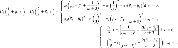 $$ no{ { {{U}_{\rm{1}}}\Big(\frac{{\rm{1}}}{{\rm{3}}}\, + \,{{\beta }_{\rm{1}}}|{{s}_{\rm{1}}}\Big)\,{\rm{ - }}\,{{U}_{\rm{1}}}\Big(\frac{{\rm{2}}}{{\rm{3}}}\, + \,{{\beta }_{\rm{1}}}|{{s}_{\rm{1}}}\Big)\, = \, \left \{ {\matrix{ \displaystyle{{{\alpha }_{\rm{2}}}{{{\left( {{{\beta }_{\rm{2}}}\,{\rm{ - }}\,{{\beta }_{\rm{1}}}\, + \,\frac{{\rm{1}}}{{m\, + \,{\rm{3}}}}} \right)}}^{\rm{2}}} \, + \,{{\alpha }_{\rm{1}}}{{{\left( {\frac{1}{3}} \right)}}^2} \,{\rm{ - }}\,{{\alpha }_{\rm{2}}}{{{\left( {{{\beta }_{\rm{2}}}\,{\rm{ - }}\,{{\beta }_{\rm{1}}}} \right)}}^{\rm{2}}} } {{\rm{if}}\,\,{{s}_{\rm{1}}}\, = \,{\rm{0}},} \cr \displaystyle{{{\alpha }_{\rm{2}}}{{{\left( {{{\beta }_{\rm{2}}}\,{\rm{ - }}\,{{\beta }_{\rm{1}}}} \right)}}^{\rm{2}}} \,{\rm{ - }}{{\alpha }_{\rm{1}}}{{{\left( {\frac{{\rm{1}}}{{\rm{3}}}} \right)}}^{\rm{2}}} \,{\rm{ - }}\,{{\alpha }_{\rm{2}}}{{{\left( {{{\beta }_{\rm{2}}}\,{\rm{ - }}\,{{\beta }_{\rm{1}}}\,{\rm{ - }}\,\frac{{\rm{1}}}{{m\, + \,{\rm{3}}}}} \right)}}^{\rm{2}}} } {{\rm{if}}\,\,{{s}_{\rm{1}}}\, = \,{\rm{1}},} }}\right} \cr \qquad \qquad \qquad \qquad \qquad \qquad \qquad \qquad \qquad \qquad \qquad \qquad \ = \left\{ {\matrix{ \displaystyle{\frac{{{{\alpha }_{\rm{1}}}}}{{\rm{9}}}\, + \,{{\alpha }_{\rm{2}}}\left[ {\frac{{\rm{1}}}{{{{{(m\, + \,{\rm{3}})}}^{\rm{2}}} }}\,{\rm{ - }}\,\frac{{{\rm{2}}({{\beta }_{\rm{1}}}\,{\rm{ - }}\,{{\beta }_{\rm{2}}})}}{{m\, + \,{\rm{3}}}}} \right]} {{\rm{if}}\,\,{{s}_{\rm{1}}}\, = \,{\rm{0}},} \cr { \displaystyle{\rm{ - }}\left( {\frac{{{{\alpha }_1}}}{9} + {{\alpha }_2}\left[ {\frac{{\rm{1}}}{{{{{(m\, + \,{\rm{3}})}}^{\rm{2}}} }}\, + \,\frac{{{\rm{2}}({{\beta }_{\rm{1}}}\,{\rm{ - }}\,{{\beta }_{\rm{2}}})}}{{m\, + \,{\rm{3}}}}} \right]} \right)} {{\rm{if}}\,\,{{s}_{\rm{1}}}\, = \,{\rm{1}}} \right. \cr} $$
In line with the discussion above regarding the definition of off-the-equilibrium-path beliefs and the incentives to manipulate, the expected payoff from dissimulating s 1 = 0 by choosing y 1 =  $$$\frac{1}{3}$$$
+β 1 after observing s 1 = 1 is unambiguously negative if β 1 > β 2. Accordingly, the only incentive-compatibility constraint that can bind in this case is dissimulating that s 1 = 1 when in fact s 1 = 0 was observed. Furthermore, note that the problem is symmetric with respect to the preference biases β 1 and β 2: the only incentive-compatibility constraint that can bind when β 1 < β 2 is identical but applies to the consideration of whether to dissimulate s 1 = 0 when s 1 was observed. Substituting this fact, one can obtain the following general necessary and sufficient condition for the existence of a separating equilibrium:
 $$ |{{\beta }_{\rm{1}}}\,{\rm{ - }}\,{{\beta }_{\rm{2}}}|\,\leq \,\frac{{{{\alpha }_{\rm{1}}}(m\, + \,{\rm{3}})}}{{{\rm{18}}{{\alpha }_{\rm{2}}}}}\, + \,\frac{{\rm{1}}}{{{\rm{2}}(m\, + \,{\rm{3}})}}. $$
In the baseline case in which Player 2 receives a single signal (that is, m = 1), Inequality 4 reduces to the following:
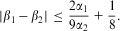 $$|{{\beta }_{\rm{1}}}\,{\rm{ - }}\,{{\beta }_{\rm{2}}}|\,\leq \,\frac{{{\rm{2}}{{\alpha }_{\rm{1}}}}}{{{\rm{9}}{{\alpha }_{\rm{2}}}}}\, + \,\frac{{\rm{1}}}{{\rm{8}}}.$$
Returning to the general case, Inequality 4 captures some key characteristics of informative decision making in this model, which we summarize in the following proposition.
Proposition 1: In any two-player environment in which the sender has discretionary authority (that is, any game γ with n = 2, E = {(1,2)}, α1 > 0 and α2 > 0), the following hold:
1. Truthful revelation is supported by larger sets of divergent preferences when the sender has greater decision-making authority (that is, as α1 grows); and
2. For any degree of preference divergence, there is a sufficiently large policy impact for the sender such that truthful revelation can be supported in equilibrium.
The two conclusions of Proposition 1 are intuitive and useful: as a player's choice of policy has a larger per se impact on his or her payoff, the net incentive to manipulate this choice so as to alter the beliefs of the other player is reduced. The second conclusion simply states that this effect is strong enough that sufficient unilateral authority can overcome the incentive to manipulate, regardless of the preference divergence between the agents. This follows from the additive separability of the players’ payoffs with respect to their policy choices.
The Three-Player Case
Moving to the analysis of three players, N = {1,2,3}, note that there are four new strategically interesting network structures. In particular, four acyclic networks connect each player in some way to at least one other agent. Up to symmetry, these four networks are:
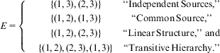 $$E\, = \,\left\{ {\matrix{ {\;\;\;\;\{ (1,3),(2,3)\} } &#x0026; {{\rm{&#x201C;Independent}}\,{\rm{Sources,\!&#x201D;}}} \cr {\;\;\;\;\{ (1,2),(1,3)\} } &#x0026; {{\rm{&#x201C;Common}}\,{\rm{Source,\!&#x201D;}}} \cr {\;\;\;\;\{ (1,2),(2,3)\} } &#x0026; {{\rm{&#x201C;Linear}}\,{\rm{Structure,\!&#x201D;\ and}}} \cr {\;\;\;\;\{ (1,2),(2,3),(1,3)\} } &#x0026; {{\rm{&#x201C;Transitive}}\,{\rm{Hierarchy}}{\rm{.}&#x201D;}} \right$$
These are each pictured in Figure 1. We now analyze the incentive-compatibility conditions for a perfectly informative equilibrium in each of these structures.Footnote 24
The four interesting three-player network structures

Independent Sources
The “independent sources” network, E = {(1,3),(2,3)}, represents a canonical situation in which one final decision maker first observes two independent (that is, simultaneous) decisions from two independently informed players. In this case, the first two players move simultaneously and affect the third player's policy choice. This case has been analyzed in the two-player case. Substituting m = 2 in Inequality 4, the necessary and sufficient condition for existence of a separating equilibrium is:
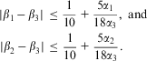 $$\matrix{ \displaystyle |{{\beta }_{\rm{1}}}\,{\rm{ - }}\,{{\beta }_{\rm{3}}}|\,\leq \,\frac{{\rm{1}}}{{{\rm{10}}}}\, + \,\frac{{{\rm{5}}{{\alpha }_{\rm{1}}}}}{{{\rm{18}}{{\alpha }_{\rm{3}}}}},\ {\rm{and}} \cr \!\!\!\!\!\!\!\!\!\!\!\!\displaystyle |{{\beta }_{\rm{2}}}\,{\rm{ - }}\,{{\beta }_{\rm{3}}}|\,\leq \,\frac{{\rm{1}}}{{{\rm{10}}}}\, + \,\frac{{{\rm{5}}{{\alpha }_{\rm{2}}}}}{{{\rm{18}}{{\alpha }_{\rm{3}}}}}. \cr $$
Note the difference between the incentive-compatibility conditions in this case versus the two-player case. For a given ratio of authorities,  $$$ \frac{{{{\alpha }_{\rm{1}}}}}{{{{\alpha }_{\rm{3}}}}} \big($$$
for which the analogous case in the two-player setting is
 $$$ \frac{{{{\alpha }_{\rm{1}}}}}{{{{\alpha }_{\rm{2}}}}} \big)$$$
, the range of preference divergence under which a perfectly informative equilibrium can be supported is strictly smaller in the independent sources network than in the two-player case if and only if the sender (Player 1) has sufficiently less authority than the receiver (Player 2 in the two-player case and Player 3 in the independent sources case). Specifically, whenever
 $$ \frac{{{{\alpha }_{\rm{1}}}}}{{{{\alpha }_{\rm{3}}}}}\, \lt \,\frac{{\rm{9}}}{{{\rm{20}}}}, $$
sustaining a perfectly informative equilibrium in the independent sources network is more demanding than in the two-player case. Notably, if the players have equal discretionary authority (α 1 = α 2 = α 3), it is easier to support a perfectly informative equilibrium in the independent sources network than in the two-player case. Furthermore, the addition of players to such a network will make the incentive-compatibility condition less binding for a player i reporting to player j with a fixed ratio of authorities  $$$ \frac{{{{\alpha }_i}}}{{{{\alpha }_j}}}\, \gt \,{\rm{0}} $$$
whenever
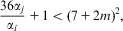 $$ \frac{{{\rm{36}}{{\alpha }_j}}}{{{{\alpha }_i}}}\, + \,{\rm{1}}\, \lt \,{{({\rm{7}}\, + \,{\rm{2}}m)}^{\rm{2}}}, $$
implying that, as long as αI > 0 and αj ≥ 0 are held fixed, there is a number of players, m × (αi,αj), such that adding additional players beyond m × (αi,αj) will not undermine (and actually bolster) the incentive compatibility of truthfulness by i.Footnote 25
The next proposition summarizes the incentive-compatibility conditions for truthful equilibrium in the independent sources network structure. The proof is omitted, as the result follows immediately from the presentation above.
Proposition 2: Suppose that three players are arranged in an independent sources network structure, E = {(1,3),(2,3)}. A truthful equilibrium with beliefs satisfying Definition 1 exists if and only if:
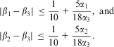 $$\matrix{ \displaystyle |{{\beta }_{\rm{1}}}\,{\rm{ - }}\,{{\beta }_{\rm{3}}}|\,\leq \,\frac{{\rm{1}}}{{{\rm{10}}}}\, + \,\frac{{{\rm{5}}{{\alpha }_{\rm{1}}}}}{{{\rm{18}}{{\alpha }_{\rm{3}}}}},\ {\rm{and}} \cr \!\!\!\!\!\!\!\!\!\!\!\!\!\displaystyle|{{\beta }_{\rm{2}}}\,{\rm{ - }}\,{{\beta }_{\rm{3}}}|\,\leq \,\frac{{\rm{1}}}{{{\rm{10}}}}\, + \,\frac{{{\rm{5}}{{\alpha }_{\rm{2}}}}}{{{\rm{18}}{{\alpha }_{\rm{3}}}}}. \cr $$
With the incentive-compatibility constraints of the independent sources network structure established, we now proceed to the common source network structure.
Common Source
A “common source” three-player network is represented by E = {(1,2),(1,3)}. In this setting, one decision maker “moves first” and his or her choice is independently observed by each of the other two players, who then make independent (simultaneous) decisions based on their own signals and anything they inferred from the first player's decision. Analysis of this case is simply a straightforward extension of the two-player case. Thus, one might apply Inequality 4 to obtain the following incentive-compatibility condition for the existence of a separating equilibrium in this case. However, while such conditions would be sufficient for existence, they would not be necessary. This is for the same reason discussed below regarding the first mover: if β 2 < β 1 < β 3 (or β 2 > β 1 > β 3), then Player 1's ability to manipulate both players with his or her policy choice is reduced.
Note that Player 1 (the common source) in this network is confronted by the same calculations with regard to possible deviations from truthfulness as Player 1 in the two-player game analyzed above: the set of potentially optimal policy choices, given that Players 2 and 3 employ beliefs as defined in Definition 1, contains exactly two possible choices: y 1∈{ $$$ \frac{1}{3} $$$
+β 1,
 $$$\frac{2}{3}$$$
+β 1}; any other choice simply results in a direct policy cost with no net “manipulation gain” in terms of the signaling value of the policy choice. Accordingly, we focus on and compare these two policy choices and let
 $$$ {\rm{\rDelta }}{{U}_{\rm{1}}} \equiv {{U}_{\rm{1}}}\big(\frac{{\rm{1}}}{{\rm{3}}}\, + \,{{\beta }_{\rm{1}}}|{{s}_{\rm{1}}}\big)\,{\rm{ - }}\,{{U}_{\rm{1}}}\big(\frac{{\rm{2}}}{{\rm{3}}}\, + \,{{\beta }_{\rm{1}}}|{{s}_{\rm{1}}}\big) $$$
. Then, presuming that Players 2 and 3 both believe that Player 1 is playing a separating strategy, Player 1's net expected payoff difference is:
 $$ {\rm{\rDelta }}{{U}_{\rm{1}}}\, = \,\left\{ {\matrix{ \displaystyle{{{\alpha }_{\rm{3}}}{{{\left( {{{\beta }_{\rm{3}}}\,{\rm{ - }}\,{{\beta }_{\rm{1}}}\, + \,\frac{{\rm{1}}}{{\rm{4}}}} \right)}}^{\rm{2}}} \, + \,{{\alpha }_{\rm{2}}}{{{\left( {{{\beta }_{\rm{2}}}\,{\rm{ - }}\,{{\beta }_{\rm{1}}}\, + \,\frac{{\rm{1}}}{{\rm{4}}}} \right)}}^{\rm{2}}} \, + \,{{\alpha }_{\rm{1}}}{{{\left( {\frac{{\rm{1}}}{{\rm{3}}}} \right)}}^{\rm{2}}} \,{\rm{ - }}\,{{\alpha }_{\rm{2}}}{{{\left( {{{\beta }_{\rm{2}}}\,{\rm{ - }}\,{{\beta }_{\rm{1}}}} \right)}}^{\rm{2}}} \,{\rm{ - }}\,{{\alpha }_{\rm{3}}}{{{\left( {{{\beta }_{\rm{3}}}\,{\rm{ - }}\,{{\beta }_{\rm{1}}}} \right)}}^{\rm{2}}} } &#x0026; {{\rm{if}}\,\,{{s}_{\rm{1}}}\, = \,{\rm{0}},} \cr \displaystyle{{{\alpha }_{\rm{2}}}{{{\left( {{{\beta }_{\rm{2}}}\,{\rm{ - }}\,{{\beta }_{\rm{1}}}} \right)}}^{\rm{2}}} \, + \,{{\alpha }_{\rm{3}}}{{{\left( {{{\beta }_{\rm{3}}}\,{\rm{ - }}\,{{\beta }_{\rm{1}}}} \right)}}^{\rm{2}}} \,{\rm{ - }}\,{{\alpha }_{\rm{3}}}{{{\left( {{{\beta }_{\rm{3}}}\,{\rm{ - }}\,{{\beta }_{\rm{1}}}\,{\rm{ - }}\,\frac{{\rm{1}}}{{\rm{4}}}} \right)}}^{\rm{2}}} \,{\rm{ - }}\,{{\alpha }_{\rm{2}}}{{{\left( {{{\beta }_{\rm{2}}}\,{\rm{ - }}\,{{\beta }_{\rm{1}}}\,{\rm{ - }}\,\frac{{\rm{1}}}{{\rm{4}}}} \right)}}^{\rm{2}}} \,{\rm{ - }}\,{{\alpha }_{\rm{1}}}{{{\left( {\frac{{\rm{1}}}{{\rm{3}}}} \right)}}^{\rm{2}}} } &#x0026; {{\rm{if}}\,\,{{s}_{\rm{1}}}\, = \,{\rm{1}}.} \right $$
The incentive-compatibility conditions for truthfulness are:
 $$ \matrix{ \displaystyle\frac{{{{\alpha }_{\rm{3}}}\left( {{{\beta }_{\rm{3}}}\,{\rm{ - }}\,{{\beta }_1}} \right)}}{{\rm{2}}}\, + \,\frac{{{{\alpha }_{\rm{2}}}\left( {{{\beta }_{\rm{2}}}\,{\rm{ - }}\,{{\beta }_{\rm{1}}}} \right)}}{{\rm{2}}}\,\geq \,{\rm{ - }}\left( {\frac{{{{\alpha }_{\rm{2}}}\, + \,{{\alpha }_{\rm{3}}}}}{{{\rm{16}}}}\, + \,\frac{{{{\alpha }_{\rm{1}}}}}{{\rm{9}}}} \right),\ {\rm{and}} \cr \!\!\!\!\!\!\!\!\!\!\!\!\!\!\!\!\!\!\!\!\!\!\!\!\!\!\!\!\!\!\!\!\!\!\!\!\!\!\!\!\!\!\!\!\!\!\!\!\!\!\!\!\!\!\!\!\!\!\!\!\!\!\!\!\!\!\!\!\!\!\!\!\!\!\!\!\!\!\!\!\!\!\!\displaystyle\frac{{{{\alpha }_{\rm{3}}}\left( {{{\beta }_{\rm{3}}}\,{\rm{ - }}\,{{\beta }_{\rm{1}}}} \right)}}{{\rm{2}}}\, + \,\frac{{{{\alpha }_{\rm{2}}}\left( {{{\beta }_{\rm{2}}}\,{\rm{ - }}\,{{\beta }_{\rm{1}}}} \right)}}{2}\,\leq \,\frac{{{{\alpha }_{\rm{2}}}\, + \,{{\alpha }_{\rm{3}}}}}{{{\rm{16}}}}\, + \,\frac{{{{\alpha }_{\rm{1}}}}}{{\rm{9}}}. \cr $$
Thus, given that beliefs satisfy Definition 1, a truthful equilibrium exists if and only if:
 $$ \left| {{{\alpha }_3}({{\beta }_3}\,{\rm{ - }}\,{{\beta }_1})\, + \,{{\alpha }_2}({{\beta }_2}\,{\rm{ - }}\,{{\beta }_1})} \right|\,\leq \,\frac{{{{\alpha }_3}\, + \,{{\alpha }_2}}}{8}\, + \,\frac{{2{{\alpha }_1}}}{9}. $$
Intuitively, Inequality 5 reduces to the necessary and sufficient condition for the existence of a separating equilibrium in the two-player case when α 3 = 0. More generally, the incentive compatibility of perfectly informative behavior is more demanding in the common source network than in the two-player case only if the bias of the “source” is either less than each of the biases of the “receivers” or greater than each of these biases. That is, only if the source's bias is similarly opposed to those of each of the receivers will the imposition of a second receiver destroy the incentive compatibility of truthfulness in a truthful equilibrium relationship between the sender and the other receiver. Intuitively, the incentive compatibility of truthfulness is never more demanding in the common source network than in the worst relevant two-player case.
Thus if the player with the “moderate bias” can truthfully signal to each of the other players in their respective two-player networks, then it is necessarily incentive compatible for that same source to truthfully signal simultaneously to those two receivers. Furthermore, such truthfulness is incentive compatible even if the source could not credibly signal truthfully to either of the two receivers in a simple two-player fashion. This fact highlights the potential power of the network as a credibility device.
If the first mover's preference is “between” those of the middle man and the final decider, then the gains from misrepresentation of his or her information are ameliorated, because while misrepresentation in one “direction” (aggressive or cautious) will benefit Player 1 in terms of the decision by, say, Player 2, that same misrepresentation will simultaneously harm Player 1 in terms of its effect on Player 3's decision.
The next proposition summarizes the presentation above and presents the incentive-compatibility conditions for the truthful equilibrium in the common source network structure.
Proposition 3: Suppose that three players are arranged in a common source network structure, E = {(1,2),(1,3)}. A truthful equilibrium with beliefs satisfying Definition 1 exists if and only if:
 $$ \left| {{{\alpha }_3}({{\beta }_3}\,{\rm{ - }}\,{{\beta }_1})\, + \,{{\alpha }_2}({{\beta }_2}\,{\rm{ - }}\,{{\beta }_1})} \right|\,\leq \,\frac{{{{\alpha }_3}\, + \,{{\alpha }_2}}}{8}\, + \,\frac{{2{{\alpha }_1}}}{9}. $$
With this analysis in hand, we now proceed to the most interesting three-player networks, the linear structure and transitive hierarchy, each of which can produce a single and uniquely most-informed decision. So long as truthfulness is incentive compatible, each of these network structures leads to one of the players’ decisions being informed by all of the players’ information. Within this setting (acyclic networks), this is the theoretical optimum in terms of maximal information aggregation.
Linear Structure
The linear structure network, E = {(1,2),(2,3)}, is a classic sequential decision-making structure.Footnote 26 Three aspects distinguish this case from the nontrivial two-player example examined earlier. First, the final decider has more information potentially available to him or her, which implies (somewhat counterintuitively) that his or her decision is in some sense less manipulable by any other individual agent. Second, the middle player can, in theory, attempt to manipulate the revelation of not only his own information, but also that of the first decision maker. Finally, the first decision maker is potentially concerned not only with how his information will affect the actions of the middle mover and the final decider, but also with how his information might affect the incentives of the middle mover to act in a truthful manner when making his or her decision.Footnote 27
The final decider's decision
Working backwards, we begin the analysis with the choice faced by Player 3 (the “final decider”). As earlier, we presume that the final decider's off-the-path beliefs are consistent with Definition 1. As opposed to the earlier analyses, however, the final decider in this situation is confronted with the need to infer more than one signal from Player 2's policy choice. Note, however, that given the equilibrium strategies under consideration, the beliefs defined in Definition 1 are relevant only if Player 2 is the deviator. That is, while Player 3 is in theory concerned about the information conveyed by Player 1 about s 1, any unilateral deviation from truthfulness by Player 1 in his or her choice of y 1 will be “washed out” by Player 2's choice, given that Player 2 is also presumed to be employing beliefs consistent with Definition 1 and using an informative strategy. Accordingly, for our purposes, if  $$$ {{y}_2} \not\in \{ \frac{1}{4}\, + \,{{\beta }_2},\frac{1}{2}\, + \,{{\beta }_2},\frac{3}{4}\, + \,{{\beta }_2}\} $$$
, this is due to a unilateral deviation by Player 2. We verify below that Player 2 indeed has no incentive to choose a policy other than these three, even if he or she wishes to deviate from truthfulness.
In equilibrium, then, the final decider will observe one of exactly four information sets, based on the number of positive signals received by Players 1, 2 and 3: 0, 1, 2 or 3. Player 3's best response in terms of choosing y 3 in each of these information sets is given by Equation 2. Letting k 3∈{0,1,2,3} denote the total number of successes observed by Players 1, 2 and 3 reduces to the following:
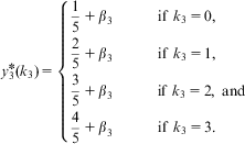 $$ y_{3}^{\ast} ({{k}_3})\, = \,\left\{ {\matrix{ \displaystyle{\frac{1}{5}\, + \,{{\beta }_3}} &#x0026; {{\rm{if}}\,\,{{k}_3}\, = \,{\rm{0}},} \cr { \displaystyle\frac{2}{5}\, + \,{{\beta }_3}} &#x0026; {{\rm{if}}\,\,{{k}_{\rm{3}}}\, = \,{\rm{1}},} \cr { \displaystyle \frac{3}{5}\, + \,{{\beta }_3}} &#x0026; \ \ \ \ \ \ {{\rm{if}}\,\,{{k}_{\rm{3}}}\, = \,{\rm{2}},\ {\rm{and}}} \cr \displaystyle{\frac{4}{5}\, + \,{{\beta }_3}} &#x0026; {{\rm{if}}\,\,{{k}_{\rm{3}}}\, = \,{\rm{3}}.} \right $$
The middle man's decision
Now consider the choice faced by Player 2 (the “middle man”). As in the discussion of the final decider above, we will demonstrate below that the first mover, Player 1, has no incentive to choose a policy other than either  $$$\frac{1}{3} $$$
+β 1 or
 $$$\frac{2}{3} $$$
+β 1. Furthermore, Player 2's beliefs are presumed to be consistent with Definition 1, so that he or she essentially has three information sets that are possible with positive probability in a truthful revelation equilibrium. These are summarized by the number of positive signals received by Players 1 and 2: 0, 1 or 2.Footnote 28
We now demonstrate that the supposition that Player 3's beliefs satisfy Definition 1 implies that Player 2 has no incentive to choose a policy  $$$ {{y}_2} \not\in \{ \frac{1}{4} + {{\beta }_2},\frac{1}{2} + {{\beta }_2},\frac{3}{4} + {{\beta }_2}\} $$$
. Abstracting from Player 1's policy choice (as it is fixed and immutable once Player 2 is faced with choosing y 2), letting
 $$$ {{\hat{s}}_1} $$$
denote Player 2's inferred value for s 1 (constructed in accordance with Definition 1) and presuming for simplicity that β 2 ≥ β 3, Player 2's expected payoff from policy choice y 2 is:
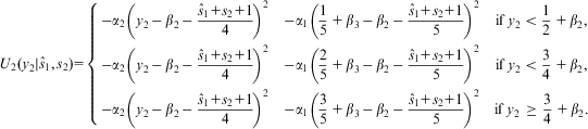 $$ {{U}_{\rm{2}}}({{y}_2}|{{\hat{s}}_1},{{s}_{\rm{2}}}) = \left\{ {\matrix{ \displaystyle {{\rm{ - }}{{\alpha }_2}{{{\left( {{{y}_2}\,{\rm{ - }}\,{{\beta }_{\rm{2}}}\,{\rm{ - }}\,\frac{{{{{\hat{s}}}_1} + {{s}_2} + 1}}{4}} \right)}}^{\rm{2}}} } &#x0026; { \displaystyle {\rm{ - }}{{\alpha }_1}{{{\left( {\frac{{\rm{1}}}{{\rm{5}}}\, + \,{{\beta }_{\rm{3}}}\,{\rm{ - }}\,{{\beta }_{\rm{2}}}\,{\rm{ - }}\,\frac{{{{{\hat{s}}}_1} + {{s}_2} + 1}}{5}} \right)}}^{\rm{2}}} } &#x0026; {{\rm{if}}\,{{y}_2}\, \lt \, \displaystyle \frac{1}{2}\, + \,{{\beta }_{\rm{2}}},} \cr { \displaystyle {\rm{ - }}{{\alpha }_2}{{{\left( {{{y}_2}\,{\rm{ - }}\,{{\beta }_{\rm{2}}}\,{\rm{ - }}\,\frac{{{{{\hat{s}}}_1} + {{s}_2} + 1}}{4}} \right)}}^{\rm{2}}} } &#x0026; { \displaystyle {\rm{ - }}{{\alpha }_1}{{{\left( {\frac{{\rm{2}}}{{\rm{5}}}\, + \,{{\beta }_{\rm{3}}}\,{\rm{ - }}\,{{\beta }_{\rm{2}}}\,{\rm{ - }}\,\frac{{{{{\hat{s}}}_1} + {{s}_2} + 1}}{5}} \right)}}^{\rm{2}}} } &#x0026; { \displaystyle {\rm{if}}\,{{y}_2}\, \lt \,\frac{3}{4}\, + \,{{\beta }_{\rm{2}}},} \cr { \displaystyle {\rm{ - }}{{\alpha }_2}{{{\left( {{{y}_2}\,{\rm{ - }}\,{{\beta }_{\rm{2}}}\,{\rm{ - }}\,\frac{{{{{\hat{s}}}_1} + {{s}_2} + 1}}{4}} \right)}}^{\rm{2}}} } &#x0026; { \displaystyle {\rm{ - }}{{\alpha }_1}{{{\left( {\frac{{\rm{3}}}{{\rm{5}}}\, + \,{{\beta }_{\rm{3}}}\,{\rm{ - }}\,{{\beta }_{\rm{2}}}\,{\rm{ - }}\,\frac{{{{{\hat{s}}}_1} + {{s}_2} + 1}}{5}} \right)}}^{\rm{2}}} } &#x0026; { \displaystyle {\rm{if}}\,{{y}_2}\,\geq \,\frac{3}{4}\, + \,{{\beta }_{\rm{2}}}} \right. $$
Note that y 2 has a direct effect on Player 2's payoff only through the first term of this function for all  $$$ {{y}_2} \not\in \{ \frac{1}{4}\, + \,{{\beta }_2},\frac{1}{2}\, + \,{{\beta }_2},\frac{3}{4}\, + \,{{\beta }_2}\} $$$
. Furthermore, among all
 $$$ {{y}_2}\,\leq \,\frac{{{{{\hat{s}}}_1}\, + \,{{s}_2}\, + \,1}}{4}\, + \,{{\beta }_2} $$$
,
 $$$ {{y}_2}\, = \,\frac{{{{{\hat{s}}}_1}\, + \,{{s}_2}\, + \,1}}{4}\, + \,{{\beta }_2} $$$
unambiguously maximizes Equation 6. Among all
 $$$ {{y}_2}\, \gt \,\frac{{{{{\hat{s}}}_1}\, + \,{{s}_2}\, + \,1}}{4}\, + \,{{\beta }_2} $$$
, Equation 6 is unambiguously decreasing in y 2 everywhere except those policy choices
 $$$ {{y}_2} \in \{ \frac{1}{4}\, + \,{{\beta }_2},\frac{1}{2}\, + \,{{\beta }_2},\frac{3}{4}\, + \,{{\beta }_2}\} $$$
. Thus if any policy y 2 offers a higher payoff to Player 2 than the (truthful) choice
 $$$ {{y}_2}\, = \,\frac{{{{{\hat{s}}}_1}\, + \,{{s}_2}\, + \,1}}{4}\, + \,{{\beta }_2} $$$
, it must be an element of the set
 $$$ \{ \frac{1}{4}\, + \,{{\beta }_2},\frac{1}{2}\, + \,{{\beta }_2},\frac{3}{4}\, + \,{{\beta }_{\rm{2}}}\} $$$
. With that in hand, straightforward calculations yield the following necessary and sufficient condition for truthful decision making to be a best response for Player 2, given Player 3's beliefs:Footnote 29
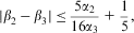
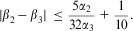 $$ |{{\beta }_2}\,{\rm{ - }}\,{{\beta }_3}|\,\leq \,\frac{{5{{\alpha }_2}}}{{32{{\alpha }_3}}}\, + \,\frac{1}{{10}}. $$
It is useful to compare this to the analogous condition (m = 2)Footnote 30 for the two-player setting:
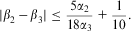 $$ |{{\beta }_2}\,{\rm{ - }}\,{{\beta }_3}|\leq \,\frac{{5{{\alpha }_2}}}{{18{{\alpha }_3}}}\, + \,\frac{1}{{10}}. $$
In the three-player, linear structure setting, the incentive-compatibility condition for the middle man is more restrictive for any ratio of authorities,  $$$ \frac{{{{\alpha }_2}}}{{{{\alpha }_3}}}\, \gt \,0 $$$
, than is the incentive-compatibility condition for the sender in the two-player setting. In other words, decision-making power has less “bang for the buck” for the middle man in the three-player setting than for the sender in the two-player situation. This is due to the fact that informational manipulation is less costly in terms of the amount of deviation from the middle man's sincerely preferred policy choice that is required to influence the final decider's decision: Player 2 can manipulate Player 3's beliefs by deviating from his or her sequentially rational policy choice by only one-fourth as opposed to one-third, as required in the two-player case.Footnote 31
The first mover's decision
Moving to the third distinctive aspect of the three-player linear structure case relative to the two-player case, consider the incentives of Player 1 (the first mover). His or her calculations are more complicated in this case than those for the sender in the two-player case, because Player 1's choice of action influences the choices of both Players 2 and 3 in a separating equilibrium within this structure. Presuming that Players 2 and 3 both believe that Player 1 is playing an informative strategy, that each of these players is employing beliefs consistent with Definition 1, and letting  $$$ {\rm{\rDelta }}{{U}_1}\, \equiv \,{{U}_1}\big(\frac{1}{3}\, + \,{{\beta }_1}|{{s}_1}\big)\,{\rm{ - }}\,{{U}_1}\big(\frac{2}{3}\, + \,{{\beta }_1}|{{s}_1}\big) $$$
, Player 1's net expected payoff is then:
 $$ {\rm{\rDelta }}{{U}_{\rm{1}}}\, = \,\left\{ {\matrix{ \displaystyle{{{\alpha }_3}{{{\left( {{{\beta }_3}\,{\rm{ - }}\,{{\beta }_1}\, + \,\frac{1}{5}} \right)}}^2} \, + \,{{\alpha }_2}{{{\left( {{{\beta }_2}\,{\rm{ - }}\,{{\beta }_1}\, + \,\frac{1}{4}} \right)}}^2} \, + \,{{\alpha }_1}{{{\left( {\frac{1}{3}} \right)}}^2} \,{\rm{ - }}\,{{\alpha }_2}{{{\left( {{{\beta }_2}\,{\rm{ - }}\,{{\beta }_1}} \right)}}^2} \,{\rm{ - }}\,{{\alpha }_3}{{{\left( {{{\beta }_3}\,{\rm{ - }}\,{{\beta }_1}} \right)}}^2} } &#x0026; {{\rm{if}}\,\,{{s}_1}\, = \,0,} \cr { \displaystyle{{\alpha }_2}{{{\left( {{{\beta }_2}\,{\rm{ - }}\,{{\beta }_1}} \right)}}^2} \, + \,{{\alpha }_3}{{{\left( {{{\beta }_3}\,{\rm{ - }}\,{{\beta }_1}} \right)}}^2} \,{\rm{ - }}\,{{\alpha }_3}{{{\left( {{{\beta }_3}\,{\rm{ - }}\,{{\beta }_1}\, + \,\frac{1}{5}} \right)}}^2} \,{\rm{ - }}\,{{\alpha }_2}{{{\left( {{{\beta }_2}\,{\rm{ - }}\,{{\beta }_1}\, + \,\frac{1}{4}} \right)}}^2} \,{\rm{ - }}\,{{\alpha }_1}{{{\left( {\frac{1}{3}} \right)}}^2} } &#x0026; {{\rm{if}}\,\,{{s}_1}\, = \,1.} \right $$
These lead to the conclusion that setting policy y 1 truthfully is a best response for Player 1 only if:
 $$ \left| {{{\alpha }_3}\frac{{2({{\beta }_1}\,{\rm{ - }}\,{{\beta }_3})}}{5}\, + \,{{\alpha }_2}\frac{{({{\beta }_1}\,{\rm{ - }}\,{{\beta }_2})}}{2}} \right|\leq \,\frac{{144{{\alpha }_3}\, + \,225{{\alpha }_2}\, + \,400{{\alpha }_1}}}{{3600}}. $$
Thus, similar to the common source network discussed earlier, the incentives for the first mover, Player 1, present a new wrinkle relative to the middle man or the sender in the two-player case. In particular, if the first mover's preference is “between” those of the middle man and the final decider, then the gains from misrepresenting his or her information are ameliorated, because while misrepresentation in one “direction” (aggressive or cautious) will benefit Player 1 in terms of the decision by (say) Player 2, that same misrepresentation will simultaneously harm Player 1 in terms of its effect on the decision by Player 3.Footnote 32
The next proposition, which follows immediately from the presentation above, summarizes the incentive-compatibility conditions for truthful equilibrium in the linear structure network.
Proposition 4: Suppose that three players are arranged in a linear structure network, E = {(1,2),(2,3)}. A truthful equilibrium with beliefs satisfying Definition 1 exists if and only if:
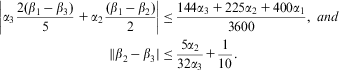 $$ \quad\displaylines{ \left| {{{\alpha }_3}\frac{{2({{\beta }_1}\,{\rm{ - }}\,{{\beta }_3})}}{5}\, + \,{{\alpha }_2}\frac{{({{\beta }_1}\,{\rm{ - }}\,{{\beta }_2})}}{2}} \right|\leq &#x0026; \frac{{144{{\alpha }_3}\, + \,225{{\alpha }_2}\, + \,400{{\alpha }_1}}}{{3600}},\ and \cr \ \ \|{{\beta }_2}\,{\rm{ - }}\,{{\beta }_3}|\leq &#x0026; \frac{{5{{\alpha }_2}}}{{32{{\alpha }_3}}} + \frac{1}{{10}}. \cr} $$
With this in hand, we now consider the final acyclic three-player network structure: the transitive hierarchy.
Transitive Hierarchy
The most complete acyclic three-player network structure is the transitive hierarchy, in which the players are uniquely ordered and each player can observe the choices of every player who has already made a decision. This represents the most transparent (acyclic) organizational structure. It turns out that the analysis of the linear form in the previous section exactly applies to this case. In particular, in a perfectly informative equilibrium, each player can infer a sufficient statistic (with respect to his or her own decision) regarding the information held by all players who have already made their policy choices. Thus, while the transitive hierarchy does provide strictly more information than the linear form (in particular, it allows the third player to determine—in a separating equilibrium—exactly which signal was received by each of the first two players), this information is strategically irrelevant in this setting, given that the beliefs satisfy Definition 1. This is established in Proposition 5 below. First, however, we discuss the beliefs held by Player 3.
Beliefs, updating and verification in multiplayer networks
The previous network structures share a common link, in that no player is ever simultaneously observing multiple policies and a player who also observed multiple signals. Put another way, no player is ever making policy after observing something that a later player will also independently observe. In the transitive hierarchy, Player 3––the final decider––observes the policy choices of both both Players 1 and 2, and Player 2 also observes Player 1's decision prior to making his or her own policy choice. Thus, this structure opens up the possibility of Player 3 “verifying” Player 2's policy decision on the basis of Player 1's decision. The key for our purposes is whether this verification ability can be leveraged by a judicious choice of beliefs by Player 3 in such a way as to make truthful revelation by Player 2 incentive compatible for a wider range of authority-bias pairs (α 2, β 2) than in the linear structure case. The answer is “no” if one considers beliefs that satisfy Definition 1, as stated in the following proposition.
Proposition 5: For any transitive hierarchy network, E = {(i,j), (i,k), (j,k)} (with i≠j, j≠k, i≠k, N = {i,j,k}) and any authorities α and any biases β, E supports a perfectly informative equilibrium in which beliefs satisfy Definition 1 if and only if  $$$ {{E}'} \, = \,\{ (i,j),(j,k)\} $$$
also supports a perfectly informative equilibrium in which beliefs satisfy Definition 1.
Proof. We proceed by deriving the incentive-compatibility conditions for the transitive hierarchy to support a perfectly informative equilibrium and show that these are identical to the corresponding conditions for the linear structure.
Beginning with Player 2, we again omit Player 1's decision (which is fixed by the time of Player 2's decision), denote the inferred value of  $$$ {{\hat{s}}_1} $$$
(which is commonly inferred by both Players 2 and 3 in this network structure) and for simplicity presume that β 2 > β 3. As with the linear structure network analyzed above, Player 2's potentially optimal policy choices are contained in
 $$$ \{ \frac{1}{4} + {{\beta }_2},\frac{1}{2} + {{\beta }_2},\frac{3}{4} + {{\beta }_2}\} $$$
. With this in hand, Player 2's expected payoff is as follows:
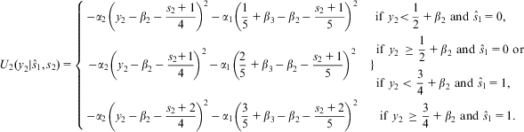 $$ {{U}_2}({{y}_2}|{{\hat{s}}_1},{{s}_2})\, = \,\left\{ \matrix{ \displaystyle{{\rm{ - }}{{\alpha }_2}{{{\left( {{{y}_2}\,{\rm{ - }}\,{{\beta }_2}\,{\rm{ - }}\,\frac{{{{s}_2}\, + \,1}}{4}} \right)}}^2} \,{\rm{ - }}\,{{\alpha }_1}{{{\left( {\frac{1}{5}\, + \,{{\beta }_3}\,{\rm{ - }}\,{{\beta }_2}\,{\rm{ - }}\,\frac{{{{s}_2}\, + \,1}}{5}} \right)}}^2} } \ \,{\displaystyle{\rm{if}} \,\,{{y}_2} \lt \frac{1}{2}\, + \,{{\beta }_2}\,\,{\rm{and}}\,\,{{{\hat{s}}}_1}\, = \,0,} \hfill\cr {{\rm{ - }}\displaystyle{{\alpha }_2}{{{\left( {{{y}_2}\,{\rm{ - }}\,{{\beta }_2}\,{\rm{ - }}\,\frac{{{{s}_2} + 1}}{4}} \right)}}^2} \,{\rm{ - }}\,{{\alpha }_1}{{{\left( {\frac{2}{5}\, + \,{{\beta }_3}\,{\rm{ - }}\,{{\beta }_2}\,{\rm{ - }}\,\frac{{{{s}_2}\, + \,1}}{5}} \right)}}^2} } &#x0026;{\left. {} \right\} \matrix{ \displaystyle{{\rm{if}}\,\,{{y}_2}\,\geq \,\frac{1}{2}\, + \,{{\beta }_2}\,\,{\rm{and}}\,\,{{{\hat{s}}}_1}\, = \,0\,\,{\rm{or}}} \hfill\hfill \cr {{\rm{if}}\,\,{{y}_2}\, \lt \displaystyle\,\frac{3}{4}\, + \,{{\beta }_2}\,\,{\rm{and}}\,\,{{{\hat{s}}}_1}\, = \,1,} \hfill } } \cr \displaystyle{{\rm{ - }}{{\alpha }_2}{{{\left( {{{y}_2}\,{\rm{ - }}\,{{\beta }_2}\,{\rm{ - }}\,\frac{{{{s}_2}\, + \,2}}{4}} \right)}}^2} \,{\rm{ - }}\,{{\alpha }_1}{{{\left( {\frac{3}{5}\, + \,{{\beta }_3}\,{\rm{ - }}\,{{\beta }_2}\,{\rm{ - }}\,\frac{{{{s}_2}\, + \,2}}{5}} \right)}}^2} } &#x0026; \displaystyle{{\rm{if}}\,\,{{y}_2}\,\geq \,\frac{3}{4}\, + \,{{\beta }_2}\,\,{\rm{and}}\,\,{{{\hat{s}}}_1}\, = \,1} \right. $$
Thus, the incentive-compatibility condition for Player 2 to truthfully reveal his or her information to Player 3 is then:
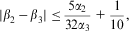 $$ |{{\beta }_2}\,{\rm{ - }}\,{{\beta }_3}|\leq \frac{{5{{\alpha }_2}}}{{32{{\alpha }_3}}}\, + \,\frac{1}{{10}}, $$
as in the linear structure case.
Turning to the first decision maker's calculations, note that the calculations for Players 2 and 3 are the same in this setting as in the linear structure network. For completeness, letting  $$$ {\rm{\rDelta }}{{U}_1}\, \equiv \,{{U}_1}\big(\frac{1}{3}\, + \,{{\beta }_1}|{{s}_1}\big)\,{\rm{ - }}\,{{U}_1}\big(\frac{2}{3}\, + \,{{\beta }_1}|{{s}_1}\big) $$$
, Player 1's net expected payoff difference between his two potentially optimal policy choices is as follows:
 $$ {\rm{\rDelta }}{{U}_1}\, = \,\left\{{\matrix{ { \displaystyle{{\alpha }_3}{{{\left( {{{\beta }_3}\,{\rm{ - }}\,{{\beta }_1}\, + \,\frac{1}{5}} \right)}}^2} \, + \,{{\alpha }_2}{{{\left( {{{\beta }_2}\,{\rm{ - }}\,{{\beta }_1}\, + \,\frac{1}{4}} \right)}}^2} \, + \,{{\alpha }_1}{{{\left( {\frac{1}{3}} \right)}}^2} \,{\rm{ - }}\,{{\alpha }_2}{{{\left( {{{\beta }_2}\,{\rm{ - }}\,{{\beta }_1}} \right)}}^2} \,{\rm{ - }}\,{{\alpha }_3}{{{\left( {{{\beta }_3}\,{\rm{ - }}\,{{\beta }_1}} \right)}}^2} } &#x0026; {{\rm{if}}\,\,{{s}_1}\, = \,0,} \cr \displaystyle{{{\alpha }_2}{{{\left( {{{\beta }_2}\,{\rm{ - }}\,{{\beta }_1}} \right)}}^2} \, + \,{{\alpha }_3}{{{\left( {{{\beta }_3}\,{\rm{ - }}\,{{\beta }_{\rm{1}}}} \right)}}^2} \,{\rm{ - }}\,{{\alpha }_3}{{{\left( {{{\beta }_3}\,{\rm{ - }}\,{{\beta }_1}\, + \,\frac{1}{5}} \right)}}^2} \,{\rm{ - }}\,{{\alpha }_2}{{{\left( {{{\beta }_2}\,{\rm{ - }}\,{{\beta }_1}\, + \,\frac{1}{4}} \right)}}^2} \,{\rm{ - }}\,{{\alpha }_1}{{{\left( {\frac{1}{3}} \right)}}^2} } &#x0026; {{\rm{if}}\,\,{{s}_1}\, = \,1.} \right $$
This leads to the conclusion that setting policy y 1 truthfully is a best response for Player 1 only if
 $$ \left| {{{\alpha }_3}\frac{{2({{\beta }_1}\,{\rm{ - }}\,{{\beta }_3})}}{5} + {{\alpha }_2}\frac{{({{\beta }_1}\,{\rm{ - }}\,{{\beta }_2})}}{2}} \right|\leq \frac{{144{{\alpha }_3}\, + \,225{{\alpha }_2}\, + \,400{{\alpha }_1}}}{{3600}}, $$
which is identical to that derived for the linear structure case (Inequality 8).
Thus, working backwards, one finds that the linear structure is equivalent to the transitive hierarchy in this setting: truthful revelation is supported in either of these communication/decision structures if it is supported in the other. ▪
Information, beliefs and comparing network structures
Before continuing, it is worth taking a moment to consider Proposition 5 in a little detail. It is in some sense surprising that the transitive and linear structure networks are equivalent from an incentive-compatibility standpoint. After all, in the transitive network structure, the final decider (Player 3) directly observes Player 1's action, whereas Player 3 must rely in essence on Player 2's report about Player 1's choice. However, as derived in Equation 9, the incentives for Player 2 are identical in the two settings. This highlights an important and somewhat subtle fact in this setting: the transparency of the transitive hierarchy implies a very strong verifiability, but this verifiability is actually irrelevant from a strategic standpoint, given that the players’ beliefs satisfy Definition 1. If one considers beliefs in which informative policy making by (say) Player 2 required that Player 2 set policy to something not equal to his or her bias, β 2, plus the true conditional expected value of θ, given Player 2's information, then the equivalence between the linear structure and transitive hierarchy does not necessarily hold. Full discussion of this topic is beyond the scope of this article for reasons of both space and focus. Specifically, as mentioned earlier (fn. 21), out-of-equilibrium beliefs are quite powerful in this setting when αI > 0 for each player i∈N. In a sense, they are “too powerful” in terms of inducing incentive compatibility of truthfulness: incentive compatibility can always be established in the baseline two-player setting, but for sufficiently divergent preferences between the two players, the maximum expected payoff from a pure strategy, separating equilibrium, can be strictly lower for the observer (Player 2) than he or she would obtain from committing to ignore the choice made by the first mover (Player 1). Establishing the exact conditions under which a pure strategy separating equilibrium is not the most-preferred equilibrium from an ex ante standpoint requires considering mixed-strategy equilibria. However the presumption that αI > 0 for each player i∈N implies that “babbling” equilibria do not exist.
With respect to the comparison at the heart of Proposition 5, a key consideration regarding the players’ beliefs (particularly those of Player 3) is the potential power of the independent observation of Player 1's policy choice, y 1, by Player 3. This independent information “allows” Player 3 to employ beliefs that use Player 2's policy choice (y 2) to affect Player 3's beliefs about only s 2, whereas, in the linear structure network, Player 3 must make inferences about both s 1 and s 2 from y 2 alone. The proposition establishes that, if Player 3's beliefs do not require Player 2 to set policy that is “more extreme” than Player 2's (decision-theoretically defined) sequentially rational choice, incentive compatibility in the linear structure is equivalent to incentive compatibility in the transitive hierarchy. Informally, this is because the “sequential rationality” aspect of Player 3's beliefs––not requiring either Player 1 or Player 2 to make decision-theoretically irrational policy choices in order to be truthfully informative to Player 3––implies that Player 3 cannot use Player 1's decision against Player 3. The degree to which Player 3's beliefs about s 2 as a function of y 2 can be conditioned on Player 1's decision, y 1, is strictly circumscribed to exactly the power of Player 3's beliefs in the linear structure network. The discussion above suggests the ambiguities inherent in proceeding to relax this “sequential rationality” restriction when comparing the ability of two different network structures to support truthful equilibria. We accordingly leave this issue for future work.
Now, with the equilibrium analyses for all four interesting network structures in hand, we briefly consider the implications of our results for the empirical study and the design of sequential networks.
Empirical Implications: Measurement And Design of Networks
The theoretical analysis in the preceding section has potentially important implications for the empirical study and design of networks. In this penultimate section, we discuss a few of these implications. The first, discussed in the following section, focuses on the empirical measurement of “networks.” As discussed in the introduction to this article, networks have attracted significant attention in various fields of political science. A common question in this broad body of research is whether and how networks “matter.” That is, how does the structure of interactions between agents affect individual and aggregate decision making? Our results indicate that the answer to this question can depend on rather fine-grained information about the network, beyond the structure of the network, and the preferences and authorities of the agents within it: the positions of the agents can matter.
The second implication of our results relates to the design of networks––both the choice of network structure and the assignment of agents to positions within a given structure. We provide a partial summary of our incentive-compatibility conditions for the linear structure networks. In particular, while the results above indicate that achieving incentive compatibility can be a “delicate” matter, Proposition 6 establishes a fundamental relationship between preferences and incentive compatibility when all players have equal, positive authority.
The Importance of Network Position
A key implication of the analysis above is that questions such as “is the linear structure network incentive compatible?” are not necessarily well posed. Specifically, there are some profiles of biases (β) and discretionary authorities (α) such that some, but not all, of the six possible linear structure networks will support informative equilibria with beliefs satisfying Definition 1.Footnote 33 This is demonstrated formally in the following example. Following the example, we provide a result demonstrating the difficulty of achieving incentive compatibility in a linear structure network.
Example 1 (Network Position Matters): Consider a three-player situation in which the players’ decision-making authorities are as follows:
 $${{\alpha }_1}\, = \,1/4,\;\;\;{{\alpha }_2}\, = \,1/2,\;\;\;{\rm{and}}\,\,\,{{\alpha }_3}\, = \,1,$$
and the players’ biases are as follows:
 $$ {{\beta }_1} = 0,\;\;\;{{\beta }_2} = 0.01,\;\;\;{\rm{and}}\,\,\,{{\beta }_3} = 0.12. $$
With these decision-making authorities and policy biases, the linear structure {(1,2),(2,3)} does not support a perfectly informative separating equilibrium. Specifically, the incentive compatibility condition for Player 2 (Equation 7) is violated, as is that for Player 1 (Equation 8):
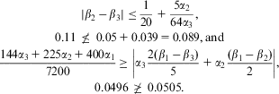 $$ \displaylines{ |{{\beta }_2}\,{\rm{ - }}\,{{\beta }_3}|\leq &#x0026; \frac{1}{{20}}\, + \,\frac{{5{{\alpha }_2}}}{{64{{\alpha }_3}}}, \cr 0.11\, \not\leq &#x0026; \,0.05\, + \,0.039\, = \,0.089,{\rm{and}} \cr \frac{{144{{\alpha }_3}\, + \,225{{\alpha }_2}\, + \,400{{\alpha }_1}}}{{7200}}\geq &#x0026; \left| {{{\alpha }_3}\frac{{2({{\beta }_1}\,{\rm{ - }}\,{{\beta }_3})}}{5}\, + \,{{\alpha }_2}\frac{{({{\beta }_1}\,{\rm{ - }}\,{{\beta }_2})}}{2}} \right|, \cr 0.0496\, \not\geq \,0.0505. \cr} $$
On the other hand, the linear structure {(2,3),(3,1)} does support a perfectly informative separating equilibrium, as:
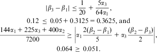 $$\matrix{\displaystyle |{{\beta }_3}\,{\rm{ - }}\,{{\beta }_1}|\leq \frac{1}{{20}}\, + \,\frac{{5{{\alpha }_3}}}{{64{{\alpha }_1}}}, \cr {\rm{0}}{\rm{.12}}\,\leq \,{\rm{0}}{\rm{.05}}\, + \,{\rm{0}}{\rm{.3125}}\, = \,{\rm{0}}{\rm{.3625}},\,{\rm{and}} \cr \displaystyle\frac{{144{{\alpha }_1}\, + \,225{{\alpha }_3}\, + \,400{{\alpha }_2}}}{{7200}}\geq \left| {{{\alpha }_1}\frac{{2({{\beta }_2}\,{\rm{ - }}\,{{\beta }_1})}}{5}\, + \,{{\alpha }_3}\frac{{({{\beta }_2}\,{\rm{ - }}\,{{\beta }_3})}}{2}} \right|, \cr {\rm{0}}{\rm{.064}}\,\geq \,{\rm{0}}{\rm{.051}}. \cr $$
Example 1 illustrates one important reason that perfectly informative equilibria can exist in one network structure but not in another isomorphic network structure. In particular, α 2 is not sufficiently large to elicit truthful information from Player 2 to Player 3.Footnote 34 To make this point as clearly as possible, note that if one leaves the players’ policy preferences, β, as in Example 1 but alters α so that α 1 = α 2 = α 3 = 1, the linear structure {(1,2),(2,3)} (indeed, every linear structure) supports a perfectly informative equilibrium. Thus, the failure of incentive compatibility in Example 1 is due entirely to the heterogeneity of decision-making authority across the players. The same possibility emerges even if the discretionary authorities are identical for the three players.Footnote 35
Partially ordering the incentive compatibility constraints
As discussed in the introduction, analyzing networks is both interesting and difficult precisely because of their complexity. Even in the small cases considered in this paper, after all, there are 25 different possible (acyclic) networks. There is no unambiguously correct notion of how to “order” them. Particularly when some of these networks do not support a perfectly informative equilibrium, this fact hinders the provision of a general “rule of thumb” about which network is best, even with an unambiguous notion of “best” such as expected (Benthamite) social welfare. The main difficulty of establishing general rules in this setting is at least partially due to the multidimensional nature of the problem. In particular, while policy is unidimensional and policy preferences are well ordered (for example, the majority rule core is nonempty and the median policy bias is comparable to a median ideal point in the classical spatial model in the sense that this bias determines the core policy), the parameter space is multidimensional in the sense that each player has a policy bias (βi) and a discretionary authority (αi). This implies that traditional ambiguities emerge when one thinks about “ordering” the parameters of different decision situations.
The next proposition considers a single-parameter family of settings within our environment. Specifically, we presume that the players have identical unilateral authority, α 1 = α 2 = α 3 = 1 and, for any nonnegative real number b ≥ 0, we suppose that the players’ preference biases are defined as:
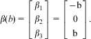 $$ \beta (b)\, = \,\left[ {\matrix{ {{{\beta }_1}} \cr {{{\beta }_2}} \cr {{{\beta }_3}} }} \right]\, = \,\left[ {\matrix{ {{\rm{ - b}}} \cr {\rm{0}} \cr {\rm{b}}}} \right]. $$
Thus, increasing b unambiguously increases the preference disagreement between the players. The next proposition characterizes the incentive-compatible network structures as a function of b. Note that because α 1 = α 2 = α 3, the social welfare (but not necessarily the existence) of a truthful equilibrium is entirely a function of the network structure, as opposed to the location of the agents within the network structure.
Proposition 6: Let α 1 = α 2 = α 3 = 1 and β = β(b) as defined in Equation 11. If any linear structure (or transitive hierarchy) is incentive compatible for (α,β), then the “left-to-right” network, {(1,2),(2,3)}, is incentive compatible.
Furthermore, if the “middle-goes-first” network, {(2,1),(1,3)}, is incentive compatible, then all linear structure networks are incentive compatible, including the “left-right-middle” network, {(1,3),(3,2)}.
Proof. The result follows from straightforward calculations. The bounds on incentive compatibility (to three digits) for the three linear structures (up to symmetry):
 $$ \{ (2,1),(1,3)\} \,\,{\rm{is}}\,\,{\rm{IC}}\,\,{\rm{if}}\,\,b\, \lt \,0.128, $$
 $$ \{ (1,3),(3,2)\} \,\,{\rm{is}}\,\,{\rm{IC}}\,\,{\rm{if}}\,\,b\, \lt \,0.153, $$
 $$ \{ (1,2),(2,3)\} \,\,{\rm{is}}\,\,{\rm{IC}}\,\,{\rm{if}}\,\,b\, \lt \,0.164. \eqno&#x25AA;$$
Proposition 6 illustrates a type of “mediator” result within our setting: when players have equal authorities and biases are symmetric around the median bias, the (two, symmetric) networks in which the player with median bias is located in the “middle man” position will be incentive compatible for a strictly larger set of such situations than any other linear structure network. Conversely, the (two, symmetric) linear structure networks with the most demanding incentive-compatible conditions are those in which the player with the median bias moves first.
This result is interesting because, among the three players, the incentive-compatibility condition for the first mover is quite clearly and intuitively least restrictive for the player with the median bias. However, placing this player first in the network structure has an indirect effect that more than offsets this salutary effect: by placing the median player first, the network is left with one of the players with an extreme bias signaling only to the player with the opposed bias. In addition, and more subtly, the middle man will have two signals in a truthful equilibrium. As discussed earlier, having additional information undermines incentive compatibility.
The relationship between network structure and social efficiency
The comparative static exercise discussed above indicates a potentially important measurement point regarding the study of networks and their impact on the efficiency of collective but decentralized decision making. In our environment, the social efficiency of any given network structure is invariant to the assignment of players to positions in the network. However, the incentive compatibility of a given network is generally sensitive to this assignment. Thus our theory highlights an important consideration for the empirical analysis of networks: social efficiency may not be measurable with respect to “network structure” because of strategic effects within the network. In other words, comparing the policy impact of two network structures is arguably an ill-posed question. As Example 1 demonstrates, the question of how effectively information will (or should) be transmitted among strategic agents within a given network depends not only on the agents’ preferences, individual levels of authority and the structure of the network they inhabit, but also on the agents’ specific locations within the network. This is arguably the most important empirical implication of our theoretical argument. Correctly analyzing the effect of network structure, preferences and authorities on information transmission requires measuring not only those factors, but also recording the individuals’ assignments to positions in the network.
Conclusion
Our model highlights an important descriptive characteristic of networked decision-making environments: when messages in networks are conveyed (partially or totally) through actions, one needs to consider the degree to which the actions have unilateral effects on their choosers’ welfare. Politically relevant networks often have this characteristic in many policy-making situations, encompassing both micro-policy (for example, individual bureaucrats’ decisions within a hierarchical organization) and macro-policy (for example, subnational governments adopting, rejecting and modifying policies in a given issue area).
Networks affect (or, perhaps, enable) information aggregation within policy environments only to the extent that messages and/or actions are to some degree sequential. Accordingly, the order of “play” in such networks can have a great impact on the strategic incentives of the players within the network. Understanding these incentives is important both in its own right and for empirical studies of the effects of network structure in political and economic decision making.
In this article, we have analyzed (very) small networks in a (very) stylized policy and informational environment. Of course, this choice is largely motivated by the complexity of the deceptively simple term “networks”: the analysis in this article hopefully demonstrates how much variety there is even when there are only three players, each player moves only once, and each player is characterized by a commonly known, unidimensional type.
There are many directions in which to expand and extend this framework even without considering larger networks. As alluded to at various points in the article, there are several intriguing mechanism design questions regarding the optimal allocation of discretionary authority (α) as well as, stepping a bit outside the framework of this article, questions about how one might select players with “appropriate” policy biases (β).Footnote 36 Finally, as we mentioned earlier in the article, a more general treatment of this setting would more closely hew to the framework studied by Galeotti, Ghiglino and Squintani (Reference Galeotti, Ghiglino and Squintani2013) and Dewan and Squintani (Reference Dewan and Squintani2012) and provide for messaging that is (partially or completely) separate from decision making. The degree to which such messaging is available is, of course, also a mechanism design problem in its own right.
Appendix
Beliefs and Incentive Compatibility
Before continuing to the general case, we prove a simple result that establishes the power of beliefs in this environment. Specifically, truthtelling is always incentive compatible for the proper specification of beliefs. The result leverages the common knowledge of authorities and preference biases (that is, the common knowledge of (α,β)). With this knowledge structure, a player can condition his or her beliefs about another player's information on the (weighted) degree of preference divergence between the two players. The next proposition demonstrates that beliefs can always be properly constructed so as to make truthful revelation through the policy choice incentive compatible.
Preposition 7: Consider the two-player setting, with N = {1,2}, E = {(1,2)} and β2 = 0.
Then, for any α1 > 0, α2 > 0 and β1∈R, there exists a belief h1( |α,β) such that truthtelling is incentive compatible for Player 1 given that this player holds beliefs h1(·|α,β) and chooses y1 sequentially rationally according to h(y1|α,β) following Player 1's choice.
Proof. Suppose that β 1 > β 2 = 0 and that there exists some  $$$ \tau \,\geq \,0 $$$
such that Player 2's sequentially rational strategy as a function of his or her signal, s 2, and the policy chosen by Player 1, y 1, given beliefs h 2(y 1|α,β), is:
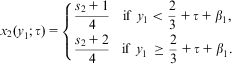 $${{x}_2}({{y}_1};\tau )\, = \,\left\{ {\matrix{ \displaystyle {\frac{{{{s}_2}\, + \,{\rm{1}}}}{{\rm{4}}}} &#x0026; {{\rm{if}}\,\,{{y}_1}\, \lt \displaystyle \,\frac{{\rm{2}}}{{\rm{3}}}\, + \,\tau \, + \,{{\beta }_1},} \cr \displaystyle {\frac{{{{s}_2}\, + \,2}}{4}} &#x0026; {{\rm{if}}\,\,{{y}_1}\,\geq \displaystyle \,\frac{{\rm{2}}}{{\rm{3}}}\, + \,\tau \, + \,{{\beta }_1}.} \right$$
Given the behavior described by Equation 12, there are only two policy choices that are both potentially optimal for Player 1 and informative to Player 2:  $$$ {{y}_1} \in \left\{ {\frac{1}{3}\, + \,{{\beta }_1},\frac{2}{3}\, + \,\tau \, + \,{{\beta }_1}} \right\} $$$
. (By “informative to Player 2” we mean that the choice of policy determines Player 2's belief, given h 2, about s 1.) Let
 $$$ y_{1}^{0} \, = \,\frac{1}{3}\, + \,{{\beta }_1} $$$
and
 $$$ y_{1}^{1} \, = \,\frac{{\rm{2}}}{{\rm{3}}}\, + \,\tau \, + \,{{\beta }_1} $$$
denote these two policies. Note that
 $$$ y_{1}^{1} \,{\rm{ - }}\,y_{1}^{0} \, = \,\frac{{\rm{1}}}{{\rm{3}}}\, + \,\tau $$$
. The expected payoff difference between these two choices is:
 $$ {{U}_1}(y_{1}^{0} |{{s}_1},{{s}_1})\,{\rm{ - }}\,{{U}_1}(y_{1}^{1} |{{s}_1},{{s}_1})\, = \,\left\{ {\matrix{ \displaystyle {{{\alpha }_2}{{{\left( {{{\beta }_2}\,{\rm{ - }}\,{{\beta }_1}\, + \,\frac{1}{4}} \right)}}^2} + {{\alpha }_1}{{{\left( {\frac{1}{3}\, + \,\tau } \right)}}^2} \,{\rm{ - }}\,{{\alpha }_2}{{{\left( {{{\beta }_2}\,{\rm{ - }}\,{{\beta }_1}} \right)}}^2} } &#x0026; {{\rm{if}}\,\,{{s}_1}\, = \,0,} \cr \displaystyle {{{\alpha }_2}{{{\left( {{{\beta }_2}\,{\rm{ - }}\,{{\beta }_1}} \right)}}^2} \, + \,{{\alpha }_1}{{\tau }^2} \,{\rm{ - }}\,{{\alpha }_1}{{{\left( {\frac{1}{3}} \right)}}^2} \,{\rm{ - }}\,{{\alpha }_2}{{{\left( {{{\beta }_2}\,{\rm{ - }}\,{{\beta }_1}\,{\rm{ - }}\,\frac{1}{4}} \right)}}^2} } &#x0026; {{\rm{if}}\,\,{{s}_1}\, = \,1,} \right $$
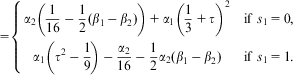 $$ \qquad \qquad \qquad= \left\{ {\matrix{ \displaystyle{{{\alpha }_2}\left( {\frac{1}{{16}}\,{\rm{ - }}\,\frac{1}{2}({{\beta }_1}\,{\rm{ - }}\,{{\beta }_2})} \right)\, + \,{{\alpha }_1}{{{\left( {\frac{1}{3}\, + \,\tau } \right)}}^2} } &#x0026; {{\rm{if}}\,\,{{s}_1}\, = \,0,} \cr \displaystyle{{{\alpha }_1}\left( {{{\tau }^2} \,{\rm{ - }}\,\frac{1}{9}} \right)\,{\rm{ - }}\,\frac{{{{\alpha }_2}}}{{16}}\,{\rm{ - }}\,\frac{1}{2}{{\alpha }_2}({{\beta }_1}\,{\rm{ - }}\,{{\beta }_2})} &#x0026; {{\rm{if}}\,\,{{s}_1}\, = \,1.} \right $$
Because β 1 > β 2, consider first the incentive-compatibility condition in the case of s 1 = 0 (this is the only one that can bind for sufficiently small τ ). In this case, truthfulness is incentive compatible with these beliefs if and only if
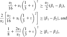 $$ \matrix{ \displaystyle\frac{{{{\alpha }_2}}}{{16}}\, + \,{{\alpha }_1}{{\left( {\frac{1}{3}\, + \,\tau } \right)}^2} \,\geq \,\frac{{{{\alpha }_2}}}{2}({{\beta }_1}\,{\rm{ - }}\,{{\beta }_2}), \cr \!\!\!\!\!\!\!\!\!\displaystyle\frac{2}{{{{\alpha }_2}}}\left[ {\frac{{{{\alpha }_2}}}{{16}}\, + \,{{\alpha }_1}{{{\left( {\frac{1}{3}\, + \,\tau } \right)}}^2} } \right]\geq |{{\beta }_1}\,{\rm{ - }}\,{{\beta }_2}|,\,{\rm{and}} \cr \!\!\!\!\!\!\!\!\!\!\displaystyle\frac{1}{8}\, + \,\frac{{2{{\alpha }_1}}}{{{{\alpha }_2}}}{{\left( {\frac{1}{3}\, + \,\tau } \right)}^2} \geq |{{\beta }_1}\,{\rm{ - }}\,{{\beta }_2}|, \cr $$
so that, as intuition suggests, for any fixed β 1 and β 2, truthfulness is incentive compatible for “sufficiently demanding” beliefs (that is, for sufficiently large values of τ ), under the supposition that Player 1 must choose between  $$$ y_{1}^{0} $$$
and
 $$$ y_{1}^{1} $$$
.
However, as alluded to above, setting τ too large can lead to a violation of incentive compatibility when s 1 = 1. In particular, Player 1 could choose his or her sequentially rational policy following s 1 = 1 even if that leads Player 2 to infer that s 1 = 0. Doing so optimally (given τ ≥ 0) involves choosing  $$$ {{y}_1}\, = \,y_{1}^{2} \, \equiv \,\frac{{{{s}_1}\, + \,2}}{3}\, + \,{{\beta }_1} $$$
. The resulting incentive-compatibility condition in this situation is based on the following expected payoff difference calculation:
 $$ \displaylines{ {{U}_1}(y_{1}^{2} |{{s}_1}\, = \,1)\,{\rm{ - }}\,{{U}_1}(y_{1}^{1} |{{s}_1}\, = \,1)\, = &#x0026; \,{{\alpha }_2}{{\left( {{{\beta }_2}\,{\rm{ - }}\,{{\beta }_1}} \right)}^2} \, + \,{{\alpha }_1}{{\tau }^2} \,{\rm{ - }}\,{{\alpha }_2}{{\left( {{{\beta }_2}\,{\rm{ - }}\,{{\beta }_1}\,{\rm{ - }}\,\frac{1}{4}} \right)}^2}, \cr \, \quad \quad\quad \quad\quad \ \ =&#x0026; \,{{\alpha }_1}{{\tau }^2} \,{\rm{ - }}\,\frac{{{{\alpha }_2}}}{{16}}\,{\rm{ - }}\,\frac{{{{\alpha }_2}}}{2}({{\beta }_1}\,{\rm{ - }}\,{{\beta }_2}), \cr} $$
so that incentive compatibility in this situation is satisfied only if:
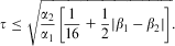 $$ \tau \leq \sqrt {\frac{{{{\alpha }_2}}}{{{{\alpha }_1}}}\left[ {\frac{1}{{16}}\, + \,\frac{1}{2}|{{\beta }_1}\,{\rm{ - }}\,{{\beta }_2}|} \right]} . $$
So, suppose that 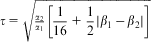 $$$ \tau \, = \,\sqrt {\frac {{{{\alpha }_2}}}{{{{\alpha }_1}}}\left[ \displaystyle{\frac{1}{{16}}\, + \,\frac{1}{2}|{{\beta }_1}\,{\rm{ - }}\,{{\beta }_2}|} \right]} $$$
. Then substituting this into Inequality 13,
 $$ \frac{1}{8}\, + \,\frac{{2{{\alpha }_1}}}{{{{\alpha }_2}}}{{\left( {\frac{1}{3}\, + \,\sqrt {\frac{{{{\alpha }_2}}}{{{{\alpha }_1}}}\left[ {\frac{1}{{16}}\, + \,\frac{1}{2}|{{\beta }_1}\,{\rm{ - }}\,{{\beta }_2}|} \right]} } \right)}^2} \geq |{{\beta }_1}\,{\rm{ - }}\,{{\beta }_2}|, $$
and letting  $$$ M \equiv \displaystyle\frac{1}{8} + \frac{{2{{\alpha }_1}}}{{{{\alpha }_2}}}{{\left( {\frac{1}{3} + \sqrt {\frac{{{{\alpha }_2}}}{{{{\alpha }_1}}}\left[ {\frac{1}{{16}} + \frac{1}{2}|{{\beta }_1}\,{\rm{ - }}\,{{\beta }_2}|} \right]} } \right)}^2} $$$
,
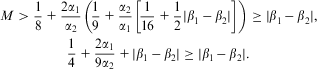 $$ \!\!\!\!\!\!\!\!\!\!\!\!\!\!\!\!\!\!\!\!\!\!\!\!\!\!\!\!\!\!\!\!\!\!\!\!\!\!\!\!\!\!\!\!\!\!\!\!\!\!\!\!\!\matrix{ M\, \gt \displaystyle\,\frac{1}{8}\, + \,\frac{{2{{\alpha }_1}}}{{{{\alpha }_2}}}\left( {\frac{1}{9}\, + \,\frac{{{{\alpha }_2}}}{{{{\alpha }_1}}}\left[ {\frac{1}{{16}}\, + \,\frac{1}{2}|{{\beta }_1}\,{\rm{ - }}\,{{\beta }_2}|} \right]} \right)\geq |{{\beta }_1}\,{\rm{ - }}\,{{\beta }_2}|, \cr \displaystyle\frac{1}{4}\, + \,\frac{{2{{\alpha }_1}}}{{9{{\alpha }_2}}}\, + \,|{{\beta }_1}\,{\rm{ - }}\,{{\beta }_2}|\geq |{{\beta }_1}\,{\rm{ - }}\,{{\beta }_2}|. \cr $$
Accordingly, setting  $$$ \tau \, = \,\sqrt {\frac{{{{\alpha }_2}}}{{{{\alpha }_1}}}\left[ {\frac{1}{{16}}\, + \,\frac{1}{2}|{{\beta }_1}\,{\rm{ - }}\,{{\beta }_2}|} \right]} $$$
implies that Inequalities 13 and 14 are simultaneously satisfied. ▪
Proposition 7 states that incentive compatibility can always be obtained, but it does not ask whether incentive compatibility is in Player 2's (that is, the “belief-holder's”) interests. A full consideration of this issue is beyond the scope of this article, but note that the “cheapest” pure strategy separating equilibrium in terms of α,β is constructed by setting t so as to satisfy Inequality 13 with equality. This value is
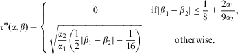 $$ {{\tau }^\ast} (\alpha, \beta )\, = \,\left\{ {\matrix{ 0 &#x0026; \displaystyle{{\rm{if}}|{{\beta }_1}\,{\rm{ - }}\,{{\beta }_2}|\leq \frac{1}{8}\, + \,\frac{{2{{\alpha }_1}}}{{9{{\alpha }_2}}},} \cr \displaystyle{\sqrt {\frac{{{{\alpha }_2}}}{{{{\alpha }_1}}}\left( {\frac{1}{2}|{{\beta }_1}\,{\rm{ - }}\,{{\beta }_2}|\,{\rm{ - }}\,\frac{1}{{16}}} \right)} } &#x0026; {{\rm{otherwise}}{\rm{}}} \right. $$
Note that Player 2's expected payoff from the pure strategy separating equilibrium that the beliefs based on Equation 12, with  $$$ \tau \, = \,{{\tau }^\ast} (\alpha, \beta ) $$$
, is:
 $$ {{U}_2}({{\tau }^\ast} (\alpha, \beta ))\, = \,{\rm{ - }}\left[ {\frac{{{{\alpha }_2}}}{{24}}\, + \,{{\alpha }_1}\left( {\frac{1}{{18}} + {{{\left( {\frac{{{{\tau }^\ast} (\alpha, \beta )}}{2}\, + \,|{{\beta }_1}\,{\rm{ - }}\,{{\beta }_2}|} \right)}}^2} } \right)} \right] $$
The following fact implies that, as the players’ preference biases diverge without bound, Player 2's expected payoff from a pure strategy separating equilibrium also decreases without bound. Accordingly, for sufficiently divergent preference biases, Player 2 will have a strict ex ante preference for a mixed-strategy (that is, partially pooling) equilibrium.
For any α 1 > 0, α 2 > 0, and β 2∈R,  $$$ {\lim }_{{{\beta }_1} \rightarrow \infty } {{\tau }^\ast} (\alpha, \beta )\, = \,\infty $$$
and
 $$$ {\lim }_{{{\beta }_1} \rightarrow \infty } {{U}_2}({{\tau }^\ast} (\alpha, \beta ))\, = \,{\rm{ - }}\infty $$$
.