1. Introduction

In many countries, home equity represents a substantial portion of the net worth of the population over age 55. Many members of this older age cohort will be required to fund their own care costs at a level exceeding their incomes. As a result, it will become more necessary for them to access the equity in their home. A standard method to do this is to sell the home, but this raises the question of where the individuals will reside. Related considerations arise as to whether it is preferable to rent or downsize, remain in the same neighbourhood or relocate. Further, there are logistical issues regarding moving, discarding, selling or otherwise disposing of property and the transaction costs that might be incurred. For many, there appears to be a desire to remain in the home, which may generate a “possession value” that is greater than the market value on sale. To accommodate the combined desires of providing access to home equity and enabling the homeowners to remain in their homes, home equity release (HER) products have been developed.

The usefulness of HER in old age has been long recognised (e.g. see Leather, 1990). Recently, more attention is being paid to the potential for HER to assist in funding long-term care (LTC) (see e.g. Hancock, Reference Hancock2000; Andrews, Reference Andrews2009, Reference Andrews2012; Northern Ireland Housing Executive, 2010; Dilnot et al., Reference Dilnot, Warner and Williams2011). However, the take-up on these products in the United Kingdom, Canada and the United States has been very limited. In this paper we describe a proposal for a competitive market framework that would help unlock housing wealth, with the specific objective of providing funds for the care expenses of an ageing population while allowing them the option to age in place. We show with the help of house price data how this structure leads to a potentially more efficient risk-sharing mechanism, and to a more transparent pricing model.

Many of the HER loans (sometimes on account of legislation) contain a provision often referred to as the no-negative-equity-guarantee (NNEG). This provision implies that if the value of the home is less than the value of the outstanding loan, there is no further obligation to repay the loan (beyond the funds received on home sale). In the United Kingdom, the NNEG is a requirement of the Equity Release Council, the main industry body in the HER sector. Various authors have suggested, based on surveyed perceptions (Overton, Reference Overton2010) or pricing models (Hosty et al., Reference Hosty, Groves, Murray and Shah2008; Li et al., Reference Li, Hardy and Tan2010), that the typical price charged for the HER loans when the NNEG is present makes the loan unattractive to the borrower and explains, at least in part, why take-up of such products has been low.

Hosty et al. (Reference Hosty, Groves, Murray and Shah2008), Ji et al. (Reference Ji, Hardy and Li2012) and Li et al. (Reference Li, Hardy and Tan2010) have developed models to price the NNEG that produce prices considerably less than those implied from rates available in the market. These pricing approaches must simultaneously model several sources of risk such as interest rate risk, house price risk and longevity risk. Furthermore, the models are estimated based on average house price returns rather than individual house prices, and they either ignore or do not directly evaluate the basis risk between an index and individual house price returns. From the lender’s perspective, the longevity risk built into the NNEG makes it necessary to exercise prudence in the size of the loan relative to the house value. As a result, the debate remains open on the necessary level of conservatism in determining the proportion of home value that may be offered as a loan.

We develop a twofold approach to this problem: we present a more transparent pricing structure that takes into account the known risks, while attempting to benefit from opportunities for efficient risk allocation. We also demonstrate this approach using individual house price data unlike existing models that are based on average returns.

The first element is the social aspect of funding the LTC expenses of retired individuals. Andrews (Reference Andrews2009, Reference Andrews2012) has suggested that the NNEG risk is more suitably borne by the state through an agency or through a public–private partnership (PPP). He suggests that if the PPP holds the NNEG risk, the remaining loan would become a relatively standard mortgage product with an uncertain exit date. Further, the PPP may lay off part of the longevity risk by entering into swap contracts with interested counterparties.

In this paper, we propose a specific structure for HER loans that involves a securitisation and a new form of loan to be offered to homeowners, at an adjustable rate based on the regional house price index (HPI). The use of HPI-based mortgages to alleviate basis risk was first proposed by Shiller & Weiss (Reference Shiller and Weiss2000). Our proposal involves the establishment of a centralised system that supports efficient sharing of risks and a transparent method for pricing HER loans. These objectives are achieved by independently pricing the NNEG consisting of basis and longevity risk, while offering HPI-linked securities backed by physical homes. It is important to note that both elements work together more effectively than in isolation. For instance, the United States has a mechanism for providing NNEG insurance via an agency, but this has not been sufficient to increase the take-up of loans because of limitations of pricing the long-term fixed-rate contracts.

Currently, most loans are offered as fixed-rate roll-up mortgages, whereby a fixed rate of interest is accumulated in the mortgage until the contract is settled. Long-term variations in housing prices are sometimes characterised as very slowly reverting to a mean trend, so a fixed-rate loan presents a further element of risk relative to house price growth. Recent literature has focused on modelling the dynamics of index-level returns. For instance, Li et al. (Reference Li, Hardy and Tan2010) fit an ARMA-GARCH model to monthly returns on the Nationwide Index of house prices, and formulate a pricing model for the NNEG as a put option based on the estimated dynamic. By unbundling the loan into an NNEG and a floating rate loan, it would be possible to have more competitive pricing owing to improved risk-sharing implications over longer time horizons.

In determining the pricing of the relative portions and demonstrating the advantages of this approach, we focus on the risk that price changes for individual houses are less than the changes in an HPI. This basis risk is a significant element of HER loan risk that has not been explicitly accounted for in previous work on pricing the NNEG. We argue that unbundling and quantifying this risk leads to greater efficiency in risk allocation. We also document a term structure in this risk and account for it in our pricing strategy.

Using a data sample from Kent County in England, we provide a more accurate estimate of the costs involved if the NNEG were provided by a PPP, based on available data. The premium for the NNEG helps determine the maximum permitted loan relative to the house valuation. Overall, our structure offers the potential for significantly raising the proportion of house value available to the elderly seeking to cover residential care costs.

Our structuring and data work also offer some additional benefits with respect to the current state of the market and the NNEG pricing approach. With respect to the data, our use of the Land Registry’s HPI, which is a repeat-sales index based on all recorded transactions, reduces the bias that arises from using a particular mortgage provider’s price indexFootnote ¹.

With respect to the investment market, we have proposed the creation of a security that would offer investors exposure to regional residential real estate prices. Given the significant variation over time of the regional distribution of house price changes (Dorling & Cornford, Reference Dorling and Cornford1995), such securities would serve to fill an important gap in the portfolios of several investors, especially pension funds interested in long-term real estate exposures. As these securities would be backed by actual homes, they could aid in a more efficient determination of prices by complementing the derivative contracts. The derivatives markets in residential real estate are still relatively limited compared with those for other assets such as equity and commodities. The absence of liquid and transparently structured securities backed by real estate implies that pricing models for derivatives, even those with linear payoffs, are complex and challenging to implementFootnote ².

It may be important to broaden the base of possible investors. Currently, the maturity profile of HER suits the liability matching requirements of insurers and specialised investors, who are the main lenders under HER schemesFootnote ³. However, the diversification potential of housing equity investments can be accessed by a wider investor base under the proposed scheme, helping alleviate any potential constraints on supply of funds.

The rest of the paper proceeds as follows. In the next section we describe the proposed structure for the HER product and related market arrangements. We present the methodology and data in section 3, and our results in section 4. Section 5 discusses an extension of the structure, with a further possibility to reallocate risks. The final section identifies some areas for future research and concludes.

2. An Alternative HER Product and its Pricing

The structure we propose involves a central intermediary, ideally in the form of a PPP. The PPP would receive applications from homeowners in need of funds to finance LTC while living in their home (i.e. ageing in place). The applicants may not require institutional LTC at the time of application, but may require funds for residential care or to modify the home to make it more accommodating to the applicant’s needs and mobility. In our simulations, we assume that the borrowers are a couple aged 65, with one partner requiring care and the other healthy.

Andrews (Reference Andrews2012) has stated several reasons that the PPP structure is desirable. The loan would include an NNEG provision. The state may be better placed to bear this risk and may also be able to use some of the homes acquired for social housing. The PPP structure provides a vehicle for the state to pass some of the risk to the private sector through a residual account, and to enhance the attractiveness and availability of the HER product.

The PPP would process the applications, which would include an appraisal of the home, a determination of the amount of equity, an assessment of its prospects for house price inflation in line with an established HPI and an underwriting of the mortality and morbidity (i.e. the LTC risk that will affect the time of sale of the home and the cessation of the loan). The PPP would then specify the maximum loan amount and the loan rate basis. Once the PPP carries out an evaluation of the NNEG, it screens investors to get the best terms for the borrower. We label the initial value of the house as V ₀, and the NNEG premium as c.

The investors forward the loan funds, and then the loan accumulates interest and an NNEG premium until the exit date. The interest consists of the floating rate basis, plus an annual charge m. This annual charge is designed to cover both an administrative fee for the PPP, and a fee representing administrative expense for the lender along with the “income component” of housing returns. The administration charge for the PPP is in respect of loan application, initiation, and underwriting and ongoing inspection and maintenance of the property. As the HPI reflects average capital growth in house prices, the loan must also include a charge representing the income generated by residential real estate investment (based on standard no-arbitrage arguments). Given the potential liquidity and lower transaction cost of the securities when managed through the proposed structure, we argue this charge should be bounded from above by the net rental yield (after ownership, maintenance, vacancy period expenses and rental management costs). This charge would be determined by the market, and thus we allow for a range of values in our simulation below.

Exit from the contract is assumed to occur when the homeowners move out because of a change in their circumstances, as specified in section 3 below. At the time of exit, investors are repaid based on the accrued loan (minus the PPP’s administrative fee), while the NNEG charge is retained by the PPP. Thus, the total return to the investor is the sum of the floating and fixed parts, and may be negative if the HPI falls below the accumulated fixed charge. While this is similar to an equity investment in housing, it would presumably outperform such an investment if rents fall in line with HPI. The roles of the various parties are described in Figure 1 and the associated cash flows are in Figure 2. This versatile structure does not preclude other forms of securitisation, such as the initiation and bundling of loans by a PPP, as long as the valuation parameters are agreed in advance.

Figure 1

Role of public–private partnership (PPP) in arranging home equity loans.

Figure 2

Cash flows associated with the proposed structure. Note: This figure explains the structure of the financing arrangement. The entire loan of L ₀ is realised from the lender, and advanced to the homeowner by the public–private partnership (PPP) at initiation (the right hand side leg). The homeowner pays the PPP the minimum of the home value at exit V _Hτ and the value of the loan determined by the change in house price index (HPI), the no-negative-equity-guarantee charge c and the “income” charge m, which is determined by the market so that L ₀ is the discounted market value of the expected cash flow to the lender (S) at time of exit τ. The PPP pays S to the lender at τ.

The standard HER loan, referred to as a roll-up mortgage, is based on a fixed interest rate. Instead, we consider writing the loan on an adjustable rate, i.e., floating rate based on the rate of return on the regional HPI. We argue that this allows for a more efficient pricing approach as it does away with a major problem of predicting long-term real estate price movements. In addition, Shiller & Weiss (Reference Shiller and Weiss2000) suggest that providing an incentive to the homeowner-borrower to maintain the property may reduce the “moral hazard” problem and result in better performing loans. This adjustable rate approach maintains the interest of the homeowner-borrower in the ongoing pricing of the loan, which may result in greater attention to property maintenance resulting in improved loan performance and a lower NNEG charge. Finally, the resulting creation of securities that is based on average regional house price appreciation would be attractive to several investor classes.

One explanation for observed conservatism in pricing HER loans is that price appreciation of a particular property may be difficult to predict. Although HPI may increase in a way that is readily modelled, a particular house may not keep pace with HPI. In previous papers on NNEG pricing, this source of risk has not been directly treatedFootnote ⁴. Shiller & Weiss (Reference Shiller and Weiss2000) consider that once equity has been released in the property, there may be little incentive for the residents to maintain the property; hence, reducing the asset value. Although they refer to “moral hazard”, a failure to maintain the property may be owing to incapacity attributable to old age or because of (fear of) lack of income. Based on an analysis of Australian data, Ong (Reference Ong2009) found that being 75 years of age or older lowers annual house price appreciation by 1.4 percentage points and further that being aged 75 or older lowers home improvement expenditure by over AUD 3,000 per year and is attributable to a decline in income in old age. Based on a review of American Housing Survey data for the period 1985–2001, Davidoff (Reference Davidoff2004) observed that annual spending by homeowners 75 and older is ∼270 USD less on routine home maintenance and 1,100 USD less on home improvement than by younger homeowners with similar homes. He observed that older homeowners realise weaker price appreciation than younger owners of similar homes in the same markets over identical horizons by ∼3%/year. These arguments support a role for the PPP in regular inspection and maintenance of the property, and justify the inclusion of a small administrative fee. We envision regular (perhaps annual) inspections of the property and a contractual agreement that the residents maintain the property to some (minimum) standard.

Overall, we argue that we are presenting a more efficient allocation for society as a whole because it gives investors the possibility of equity-like exposure to residential real estate without the hassles of ownership, while it offers borrowers the access to necessary funds without the loss of “possession value”. While the latter objective is met by any HER product, the joint achievement of the two objectives at lower cost suggests the existence of an economic surplus that would be of interest to policymakers.

3. Methodology and Data

In this section, we describe in detail the methodology and data used.

3.1. Model and simulation setup

Let H be the reference HPI, and let the annualised return on H be $$\overline{h} $$ . The investors thus expect to receive $$\bar{h}{\plus}m$$ on the loan (L ₀). The NNEG charge c must then account for the fact that individual borrower house price inflation (h _i) may not match $$\overline{h} $$ . If the value of the loan exceeds the price of the house on exit, the PPP is responsible for the difference. The value of the securities would also depend on the actual time of exit τ. Owing to the nature of this contract (i.e. for financing LTC expenses at home) we can consider τ to be independent of $$\left\{ {h_{{i,\,t}} } \right\}_{{t\geq 0}} ;i=1,...,N$$ where t represents the time passed since initiation of the loan. The expected time of exit at initiation of the contract is denoted τ ₀.

The initial loan can then be written as

$$L_{{i,\,0}} =\lambda E_{0} \left[ {V_{{i,\,\tau _{0} }} \exp \left( {{\minus}\int_{t=0}^{\tau _{0} } (\overline{h} _{t} {\plus}m{\plus}c)dt} \right)} \right]$$

where $$\lambda \in \left( {0,1} \right]$$ is a policy-based proportion and V _i the value of the home. We will henceforth assume that λ is 1 – note that this would imply the highest value for c. Note also that the “moral hazard” argument of Shiller & Weiss (Reference Shiller and Weiss2000) and their recommendation to use an index as a reference rate for the loan has the additional requirement that the borrower must still have sufficient equity in the house, suggesting that λ<1 would then be more appropriate. However, we have assumed the administration fee and related provisions would substitute as an alleviation mechanism. The entire value of the loan L _i,0 is realised from investors, and thus S _i,0=L _i,0.

At exit τ the PPP receives $$\min \left[ {L_{{i,\,0}} \exp \left(\int {_{t=0}^\tau (\overline{h} _{t} {\plus}m{\plus}c)dt} \right),\,V_{{i,\,\tau }} } \right]$$ , which is the lesser of the accrued loan and the value of the house. In turn, the PPP must pay the investors $$S_{{i,\,\tau }} =S_{{i,\,0}} \exp \left(\int {_{t=0}^\tau (\overline{h} _{t} {\plus}m)dt} \right)$$ less the administration charge. In our simulations below, we assume this administration charge to be 20 basis points/year and add it to m.

The value of the property at τ is 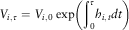$$V_{{i,\,\tau }} =V_{{i,\,0}} \exp \left( {\int_0^\tau h_{{i,\,t}} dt} \right)$$ . Suppose we let $$E_{0} \left[ {V_{{i,\,\tau _{0} }} \exp \left({{\minus}\int _0^{\tau _{0} } \overline{h} _{t} dt} \right)} \right]=V_{{i,\,0}} $$ . Then,

(1) $$L_{{i,\,0}} =V_{{i,\,0}} \exp \left( {{\minus}\left( {m{\plus}c} \right)\tau _{0} } \right)$$

Equation (1) determines the loan value relative to the initial house value.

We can then show that the NNEG charge should satisfy $$c\tau _{0} \geq {1 \over N}\mathop{\sum}\limits_i {\int_0^\tau \left( {\overline{h} _{t} {\minus}h_{{i,\,t}} } \right)dt{\plus}m\left( {\tau {\minus}\tau _{0} } \right)} $$ .

This shows that the outcome for the PPP depends on $$\left\{ {\overline{h} _{t} {\minus}h_{{i,\,t}} } \right\}_{{t=0}}^{\tau } $$ and the extent to which the actual date of entry into LTC exceeds the expected date (the longevity risk).

For the simulation, our approach is to determine certain conditions under which an HER loan would continue or would result in sale of the house underlying the loan. Ji et al. (Reference Ji, Hardy and Li2012) developed a semi-Markov multiple state model for reverse mortgage terminations. They consider three different modes of reverse mortgage termination: death, entrance into a LTC facility, and voluntary prepayment; and also model the event-triggered dependency between the lifetimes of a husband and wife. They discuss Markov approaches to joint-life mortality, which is relevant to reverse mortgage terminations, as the termination is frequently affected by events that happen to a couple. In this paper, we follow their mortality modelling and parameterisation. We use a Gompertz mortality model (μ _x=BC ^x) parameterised according to Ji et al. (Reference Ji, Hardy and Li2011, table 3). We follow their adjustments to mortality probabilities to reflect the “bereavement effect” associated with death of a spouse.

We further assume that applicants eligible for the HER loan through the PPP would be couples of approximately age 65 at a time when one of the couple has requirements for some form of care expenditure. We use a Markov model to estimate the likelihood of a change in status that would result in the home having to be sold and the loan repaid, in each year. Once a person requires care we do not permit the possibility of recovery. We consider the following end of year states of the healthy partner X and care-requiring partner Y:

1. 1. No change in state of X and Y

2. 2. X healthy, Y deceased

3. 3. X requires care, Y requires care

4. 4. X deceased, Y requires care

5. 5. X requires care, Y deceased

6. 6. X deceased, Y deceased

A change to States 3, 4, 5 or 6 would result in sale of the house and settlement of the loan. If the couple remains in State 1 the loan continues. If the transition is to State 2 we assume that the loan continues and calculate the probability that in subsequent years X will be in the states:

1. 7. X healthy

2. 8. X requires care

3. 9. X deceased

Transitions to States 8 or 9 would result in sale of the home. An alternative assumption would have been to assume voluntary loan repayment on transition to State 2. We have not assumed any prepayments as our focus is on the issue of funding LTC at home. The equity position in the home will remain relative to the overall value of the home, so unlike traditional HER products, market-timing decisions by borrowers do not pose as big a risk to lenders under our structure. Lenders receive a rate of return tied to the index and can reinvest in the index at the time of prepayment.

The expression for the calculation of the expected date of house sale is

(2) $$\mathop{\sum}\nolimits_{j=1}^\omega {j\Big[\mathop{\prod}\nolimits_{{m=0}}^{{j{\minus}1}} C_{m} A_{j} {\plus}\mathop{\sum}\nolimits_{k=1}^{j{\minus}1} {x_{k} \mathop{\prod}\nolimits_{{l=0}}^{{k{\minus}j}} } C_{i} B_{j} \mathop{\prod}\nolimits_{{n=k{\plus}1}}^{{j{\minus}1}} D_{n} \Big]} ,\,{\rm with}\,C_{0} =1$$

where subscripts represent time, C the probability that there is no change from the original state (i.e. remain in State 1), x the probability that the state changes to X healthy Y deceased (State 2), A the probability that both partners are deceased and/or require care at the end of the year (States 3, 4, 5 or 6), B the probability that the single healthy X dies or requires care by the end of the year (States 8 or 9), D the probability that the single healthy X continues in that state (State 7). The states are determined at the end of the year. The associated probability tree for the first 4 years is shown in Figure 3.

Figure 3

Probability tree for the first 4 years after loan initiation. Note: When the loan is initiated, X is the healthy partner and Y is the partner requiring care expenditures at home. C represents the probability that there is no change from the original state; x represents the probability that the state changes to X healthy Y deceased; A represents the probability that both partners are deceased and/or require care at the end of the year; B represents the probability that the single healthy X dies or requires care by the end of the year; D represents the probability that the single healthy X continues in that state. The states are determined at the end of the year. The associated probability tree for the first 4 years is shown.

In the event of sale, we compare the appreciation of the index derived from the HPI, which would have been used to price the loan to the likely increase in the individual house’s value. Differences in price that result in the NNEG provision being triggered are captured. One million simulations are run to estimate the likelihood and timing of the triggering of the NNEG. We then calculate break-even NNEG premiums using different discount rates. Based on the break-even NNEG premiums we are able to determine an appropriate annual charge for the NNEG. We repeat the process but assume the loans were made by instalments rather than having an outstanding balance from initiation to final repayment.

For the annual charge, we consider a range of values ranging between 0 and 400 basis points annually, plus the 20 basis points administration charge payable to the PPP. As a comparison, a recently launched investment product known as an income Housa (Castle Trust, 2014) in United Kingdom offers investors a return equal to the change in a national HPI plus 2%–3% annual income over a fixed term of between 3 and 10 years.

The choice of 20 basis points for the administration charge as mentioned above is arbitrary, but given its simple interpretation, the impact of changing this charge on the total loan eligibility is straightforward to calculate and not very significant from the perspective of our simulation.

3.2. Data

We purchased data from the UK Land Registry regarding house sales during the period 1 January 1995 to 31 December 2011 for post codes in the county of Kent, England, CT1 and CT2, which correspond to the Canterbury area, and ME8, which corresponds to the Medway area. We then matched and filtered the data, so that only houses that were sold at least twice during the period were included. We use the first sale to determine the market price and subsequent sales to determine individual house returns over the relevant time horizon. We then compare this return to the change in the HPI for the same period pertaining to the county of Kent, as calculated and published by the Land Registry (2013). This gives us a set of data points representing the difference between actual house price increases and the county-wide HPI.

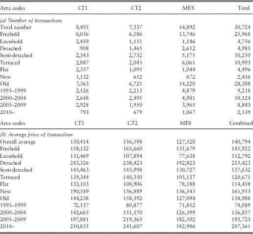
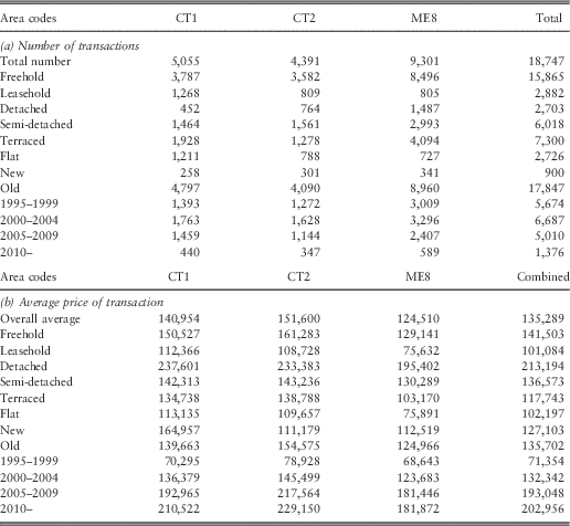
The data set received from the Land Registry contained 30,724 transactions, which included 18,747 repeat transactions, i.e., more than one transaction on the same property. There were multiple repeat transactions for some properties. Tables 1 and 2 summarise the data with respect to the full data set and the data set of repeat transactions. As the 18,747 figure includes the initial sale, the number of annualised returns in respect of repeat transactions was 10,555. While using this data set, several filters are necessary, including cases where the type of the property is changed between transactions. As an example, this can happen because of conversion of a house into several apartments at the same address. We also need to eliminate apparently unreasonably high returns that arise from significant price changes, typically when two transactions are recorded close together, e.g., 1 day apart.

Table 1

Complete data set: (a) number and (b) average price (in GBP) of transactions by area code, type and period.

Table 2

Data for repeat transactions: (a) number and (b) average price (in GBP) of transactions by area code, type and period.

From Tables 1(a) and 2(a) it can be seen that the number of transactions is approximately equal for the Canterbury (post codes CT1 and CT2) and the Medway (post code ME8) subsets of the data. The average price for the repeat transactions is less than the average price for the full data set as per Tables 1(b) and 2(b). In addition, the average price for Canterbury transactions exceeds that for Medway transactions.

As the data is for the period 1 January 1995 to 31 December 2011, the repeat transaction data is more voluminous during the middle portion of this time period and more closely matches the transaction volumes for all transactions from the 2000s onwards. This occurs because if an original sale took place before the period started the first sale would not be treated as a repeat sale. This effect can be seen in Figure 4.

Figure 4

Monthly transaction volumes for CT1, CT2 and ME8 area codes and the overall house price index (HPI) for Kent, England.

We considered adjusting for the “under representation” in the earlier years by excluding the first 5 years of observations. However, HPI increased very strongly between 2000 and 2008, when volumes were heavy. We decided not to make this adjustment because it would lead to loss of observations from a relevant period with different market patterns.

With respect to the period after 2008, when volumes decreased substantially, an argument could be made that during this period there may have been sales desired but insufficient buyers. This is a potential problem with pricing the NNEG associated with the HER loan for two reasons. House sales under HER loans are triggered by biometric events and not house price appreciation and during a period of lower volume there may also be lower prices. However, from Figure 4 it can be seen that the repeat sales in our study capture a relatively consistent proportion of the index volume; hence, no adjustment was made for this consideration.

The strong overall increase in HPI shown in Figure 4 masks the extreme variability in monthly HPI experienced over the time period, which is shown in Figure 5(a). Given this variability the data period is useful for pricing the NNEG.

Figure 5

(a) Monthly house price index (HPI) returns. (b) Autocorrelation in monthly HPI returns.

It is also noteworthy that monthly HPI shows significantly persistent autocorrelation as shown in Figure 5(b) (see Kuo, Reference Kuo1994 for results from a different time period and region). This may prove challenging for individuals using models that are not based on historical data. The ARCH or GARCH models used by other authors (e.g. Li et al., Reference Li, Hardy and Tan2010) will have to account for autocorrelation for long periods, well in excess of 3 years. Our non-parametric approach calculates the price of the NNEG based on the actual matched sample data over a long period of time. Furthermore, the autocorrelation shown in Figure 5(b) is more persistent than noted by Li et al. (Reference Li, Hardy and Tan2010). They used the Nationwide Price Index and found that a strong autocorrelation effect lasts for ∼2 years. Hosty et al. (Reference Hosty, Groves, Murray and Shah2008) also analysed the Nationwide Index and found that the autocorrelation and volatility vary by region. They do not cite figures separately for the county of Kent so we are not able to make further comparisons to their work.

We then compared the difference in annualised returns between the individual house price inflation to the HPI between transaction dates. The transaction data has exact dates, but the HPI is calculated at month ends. We used linear interpolation between consecutive HPI values to be able to match the period between transaction dates. We decided to remove the most extreme values of the differences in annualised returns between individual house price inflation and HPI from the subsequent analysis. For the highest 5% of the annualised return differences (i.e. above the 95th percentile) we substituted the value for the 95th percentile and for lowest 0.5% of the annualised return differences we substituted the value for the 0.5th percentile, i.e., we winsorised both tails, but were more conservative about substituting extreme negative observations than extreme positive ones.

The results of the winsorisation process are evident in the size of the extreme left and right hand bins of Figure 6. From the shape of the histogram it can be seen that the return differences have a positive median. Although we cannot be certain of the reason for this effect, we suspect that it is because of our data being in respect of sales in relatively desirable urban centres in the county, whereas the HPI is calculated based on all sales within the county.

Figure 6

Histogram of winsorised return differences between individual homes and house price index (HPI).

To remove the impact on pricing of having a positive mean, we recalculated the distribution of return differences by subtracting the mean difference from the data underlying Figure 6. This resulted in the distribution shown in Figure 7, which we used to price the NNEG. Note the long left tail.

Figure 7

Demeaned differences, both raw and maintaining duration. Note: We present the histogram of demeaned differences between individual house price returns and house price index (HPI) returns over the same period based on all available matched repeat-sales transactions in the data set. We also include a “duration adjusted” histogram that shows the distribution that would arise if we observed the return changes at the time of exit of a contract. This duration effect reflects the increased mass in the centre of the distribution from a longer duration of long-term care borrower tenure than average market tenure implied by our sample.

In our analysis of the data of annualised return differences we noted a duration effect as shown in Figure 8, which is based on the data underlying Figure 6. The bolder horizontal lines at the top and bottom of the Figure 8 result from the winsorisation of the data. It is particularly interesting to note that as the time between transactions increases, the variability of return differences reduces. However, it takes at least 10 years before it might be considered stable. In the United States, the Federal Housing Finance Administration (FHFA) publishes estimates of the dispersion of house prices around the index by modelling the house prices as a diffusion whose variance naturally grows over time, but at a decreasing rate. This is consistent with our findings that the annualised deviations fall over time, though the effect is more pronounced for our sample. Our approach instead is non-parametric, so we do not estimate the dispersion as a smoothed function of time. Instead, we use randomly drawn returns with matched holding periods in our simulation, thereby avoiding the need to model this duration effect. Figure 9 presents a comparison of duration-based dispersion in our data with FHFA estimates of volatility for the state of Rhode Island. Rhode Island has a small population and so may provide an appropriate comparison to the data for the communities in Kent County on which this paper is based.

Figure 8

Annualised return differences by time between transactions.

Figure 9

Annualised standard deviation of individual house prices around the index: comparison with model estimates from Rhode Island, United States. Note: We plot the Federal Housing Finance Administration’s (FHFA) estimates for volatility (annualised) over a 15-year horizon based on a diffusion model alongside the estimates from our data for Canterbury and Medway. The standard deviation in our sample is higher and falls faster than the experience in Rhode Island implied by FHFA estimates.

As our data is in respect of HPI in a county in England, it would be desirable to have information for England regarding incidence rates of entry into care and duration in care once entered. We could not find any publicly available sources that provided this information for the local population. However, the Intercompany Study Report (Gagne et al., Reference Gagne, Corliss, Campbell, Ho, Koklefsky, Lucas, Oberman-Smith, Perry, Purushotham and Shaughnessy2011) published by the Society of Actuaries is an important source of data on LTC incidence for developed western countries. Figure 5(a) of that report shows the ratio of female-to-male incidence with respect to care requirement to be 149% for ages 65–69. Accordingly, we assumed that 60% of the applicants would be a couple with a healthy male and a female requiring care expenditures and that 40% of the applicants would be a couple with a healthy female and a male requiring care expenditures. To evaluate the probabilities of a person requiring care at later ages, we used the incidence rates shown in Figure 4 of the same report (for Unlimited Benefit Period), modified by the rates by gender.

4. Results

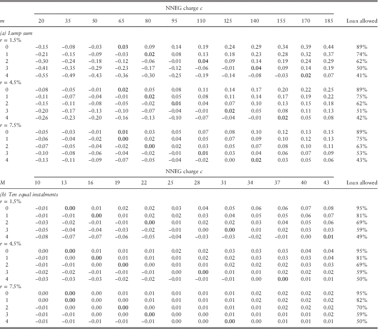
Table 3(a) presents the payoffs to the PPP for three different interest rates when the loan is disbursed as a lump sum at loan initiation. The lowest level of c for each m that results in a non-negative payoff is highlighted in bold. The farthest column to the right is the backed-out maximum loan value as a percentage of initial property value.

Table 3

Payoffs to the public–private partnership (PPP) used to determine break-even no-negative-equity-guarantee (NNEG) c for each value of m and r when the loan is advanced as a (a) lump sum and in (b) ten equal instalments.

Note: For three different interest rate environments, we calculate the payoff to the PPP for a range of values of m and c. The numbers in bold are the first level of c at which the payoff is positive. The corresponding break-even proportion of house value that may be loaned is in the far right column. m is in percentage points while c is in basis points. The value for loan allowed has been calculated as per equation (1) in the text, including a 20 basis point administration charge/year in addition to the m shown.

First, the loan allowed in this setting is found to range from 89% at the higher end to 41% at the lower end. The break-even outcomes occur for an annual NNEG charge of ∼65 basis points when m equals 20 basis points to a range of 140–170 basis points when m equals 420 basis points. An increase in the size of m (a fixed component) makes the charge more sensitive to the interest rate.

In Table 3(a) we can see that the loan value is relatively insensitive to the interest rate level at loan initiation. In addition, as expected, when m increases, c increases as well. This is consistent with m being fixed for the tenure of the loan and thus reflecting greater HPI risk and longevity risk.

In Table 3(b) we present the case when the loan is disbursed in ten equal annual instalments. The break-even range for c shifts down to the region between 13 and 37 basis points/annum. When m is at 20 basis points, c is 13 basis points, and the possible loan ratio rises to 95%.

Note that the maximum loan allowed is about 50% when the annual fixed charge in excess of the NNEG charge is 420 basis points, leading to a total charge exceeding 450 basis points/annum. This result suggests why consumers may find the HER loan pricing unattractive; 420 basis points is a considerable annual charge in excess of the NNEG fee for such a financial product.

These results are significant for a number of reasons. First, the results are consistent with those reported by Li et al. (Reference Li, Hardy and Tan2010), who used a model and very different assumptions for interest and mortality. Second, the results show that the maximum loan values available to borrowers could be made attractive through an efficient pricing and administration mechanism under which the loans were based on a floating rate. This is undoubtedly a factor in explaining the low take-up rates for HER loans. Third, even greater loan amounts could be made if the loan is disbursed in instalments.

5. Discussion and Further Possibilities

In this section we discuss some further issues with the design of the loan structure and its wider applicability. One of the concerns for which our data is inadequate is a question of whether the risk of under-maintenance of the homes discussed in section 2 has been completely accounted for. Our baseline model assumes that the maintenance is carried out by the homeowner because of the incentive effects of tying the repayment rate to the index; although, elderly or partially disabled homeowners may find this difficult or expensive. In some cases, the PPP may choose to raise the administrative fees to account for maintenance expenditures carried out by the PPP itself. More complexity can be introduced into contracts based on standards and costs of maintenance in different regions. This could be priced by our model, but is not the focus of this paper.

There is also a question of wider applicability of the proposed structure. Our focus in this paper is on the provision of financing for LTC, as the issue will increasingly challenge policymakers. This focus allows us to suggest government involvement, a specific funding structure and policy response. Moreover, in the context of LTC considerations, it is more reasonable to model the behaviour of homeowners as seeking equity release in order to age in place and manage daily expenses, including care costs, and not for the purpose of seeking an additional way to invest in the future variability of house prices and of differences in their individual house’s price and the index.

However, the potential for a similar lending and securitisation structure open to a wider class of borrowers is worth evaluating carefully. A more generally available HER product based on our proposed structure may not be appealing to policymakers and would thus require a different level of market co-ordination and more complex rules and modelling considerations that are beyond the scope of this paper.

In addition, products such as home reversion agreements currently allow investors to purchase equity in individual homes, and to that extent they are similar to our proposals. In home reversion agreements, individual homeowners effectively sell a certain amount of equity in their home at a deeply discounted price that reflects their life expectancy and house price forecasts. The high discounts again reflect the idiosyncratic risks from individual properties and the combined risks built into the NNEG that affect traditional fixed-rate HER products. Any alternative structure that would match our proposal would be based on the principle of unbundling and reallocation of risks, thereby attracting funders wishing to be exposed to residential real estate as an asset class.

Finally, a further possibility exists for policymakers to lay off more risk. In the United States, the FHFA has recently made successful efforts to pass some credit risk to private parties (Goodman et al., Reference Goodman, Yang and Landy2013). This shows that it may be further possible for the state to pass some risk from an NNEG to the private sector through the PPP’s residual account.

A second securitisation of the residual account (in the PPP) is possible in order that private investors could share the risk of the NNEG. Income to the residual account occurs from:

• ∙ NNEG premiums incorporated into the loans;

• ∙ the fee charged for administrative, maintenance and servicing included in the loans; and

• ∙ settlement payments when the residual account is negative.

Payments from the residual account occur from:

• ∙ payments required by the NNEG when the loan value exceeds the house value on sale;

• ∙ expenses incurred by the PPP for administration, maintenance and servicing; and

• ∙ dividends to investors to share any profits in the residual account.

The payments on the NNEG arise because the loan value exceeds the house value on sale. The date at which this comparison takes place is on the sale of the house due to either institutionalisation or on death. Hence, the risk associated with the NNEG includes both morbidity and mortality. Where the house price at sale exceeds the value of the loan, the homeowner would have the option to receive the excess on sale or to seek a mortgage for the loan amount and retain the home. If the expected sale price is close to the loan value, and if the property were deemed suitable for social housing, the homeowner might agree to transfer ownership to the PPP and reduce sale-related costs, so that the home could be used for social housing.

Andrews (Reference Andrews2012) discusses this type of product design and proposes that differences between the expected date of entry into care and the actual date of entry into care could be handled by a swap. If this were done then the securitisation of the residual account would be a pure play on the efficiency of the loan process and deviations in actual house price improvement from the HPI. Some financial institutions might prefer such a “purer” securitisation; hence, the available market for participation in these financial transactions might be broadened by having both a swap and a securitisation, which could lead to greater efficiency. In the absence of such a swap, any differences between expected and actual date of entry into care would be part of the residual account.

6. Conclusion

We have shown that disbursing the loan in instalments decreases the required NNEG premium and could be used as a way to increase the maximum loan value, potentially resulting in loan values of up to 95% of appraised value. It is important for authorities or private institutions to organise the collection of more data that would allow for greater precision in pricing, and reduce the range of uncertainty. However, the results are so strikingly different from the pricing that appears to be available in the market today that greater consideration regarding how the HER loan is structured is warranted.

Our findings have implications for HER products in general and especially for HER products related to LTC. Davidoff (2010) suggests that HER may affect demand for LTC insurance and is a substitute for such insurance. Our proposed structure may also be generalised and widened to offer an alternative approach to the challenges recognised by Shiller & Weiss (Reference Shiller and Weiss1999) in terms of offering home equity insurance to homeowners.

Population ageing is increasing the interest in LTC provision. Various reports (e.g. Sutherland, Reference Sutherland1999) have recommended that England provide a better organised system of LTC provision, but their recommendations have not been implemented fully because they have been judged too costly, among reasons given. Following the most recent commission’s report (Dilnot et al., Reference Dilnot, Warner and Williams2011), the government has proposed legislation that revises the available financial support regarding LTC. In view of this, the paper has a practical application. It proposes a specific HER loan in respect of LTC costs that might be provided by a PPP, where the loan administration would be highly efficient and the NNEG risk could be borne by private investors through a securitisation. This would support the government’s proposed legislation and help address increasing concerns about LTC financing for the elderly.

The market associated with the provision of the NNEG exhibits unfulfilled potential. If the market structure demonstrated in this paper were adopted, we expect that a more competitive market in HER loans would be available.