





1. Introduction
Mantle convection plays a central role in shaping Earth’s long-wavelength surface features, including enigmatic structures known as superswells – broad topographic uplifts such as those observed in the South Pacific and Southern Africa (Davaille Reference Davaille1999a ; Tackley Reference Tackley2000). These features are often attributed to the presence of thermochemical plumes and complex convective interactions in Earth’s mantle. Analogous interfacial behaviours, including large-scale deformation and fragmentation, arise in many natural and industrial systems where turbulent multiphase flows are driven by thermal gradients. Examples range from ocean–atmosphere interactions (Neelin, Latif & Jin Reference Neelin, Latif and Jin1994) to boiling in cooking (Dhir Reference Dhir1998), to experimental studies of mantle analogues (Davaille Reference Davaille1999b ).
In these systems, layered convection introduces rich interfacial dynamics, where the interface may deform into dome-like structures or fragment into droplets depending on competing physical forces. For example, inhomogeneous composition in the mantle leads to convective instabilities and interface deformation (Davaille Reference Davaille1999a ), while raindrop fragmentation during descent reflects an inertial–thermal buoyant balance (Villermaux & Bossa Reference Villermaux and Bossa2009). Understanding these transitions requires identifying the governing dimensionless parameters and quantifying the balance among buoyancy, inertia, viscosity and surface tension (Liu et al. Reference Liu, Chong, Wang, Ng, Verzicco and Lohse2021a ; Le Bars & Davaille Reference Le Bars and Davaille2004b ).
A canonical model for investigating these dynamics is Rayleigh–Bénard (RB) convection in two immiscible fluid layers (Ahlers, Grossmann & Lohse Reference Ahlers, Grossmann and Lohse2009; Lohse & Xia Reference Lohse and Xia2010; Xie & Xia Reference Xie and Xia2013), where the system is heated from below and cooled from above. The single-phase RB is controlled by the Rayleigh number (
 $\textit{Ra}$
) and Prandtl number (
 $\textit{Pr}$
). First,
 $\textit{Ra}$
quantifies the intensity of thermal driving and is expressed as
 $\textit{Ra}=\alpha g\Delta TH^{3}/(\nu \kappa )$
, where
 $\alpha$
is the thermal expansion coefficient,
 $g$
the gravitational acceleration,
 $\nu$
the kinematic viscosity and
 $\kappa$
the thermal diffusivity. Meanwhile,
 $\textit{Pr}$
characterises the fluid’s momentum-to-thermal diffusivity ratio through
 $\textit{Pr}=\nu /\kappa$
. In two-layer RB convection, additional dimensionless parameters emerge from differences in material properties, including density, viscosity, conductivity, thermal expansion and heat capacity. Of particular importance are the Weber number
 $\textit{We}=\rho U^2H/\sigma$
, which measures the ratio of inertial to surface tension forces, and the buoyancy number
 $B = \Delta \rho / (\rho \alpha \Delta T)$
, representing the ratio of compositional to thermal buoyancy (Richter & Johnson Reference Richter and Johnson1974; Richter & McKenzie Reference Richter and McKenzie1981). Here,
 $U = \sqrt {\alpha gH\Delta T}$
is the free-fall velocity,
 $\sigma$
is the surface tension coefficient,
 $\rho$
is the density of the lower fluid, and
 $\Delta \rho$
is the density difference between the lower and upper fluids.
Earlier work on two-layer convection, largely motivated by mantle flow, typically assumed an infinite
 $\textit{Pr}$
(Davaille Reference Davaille1999a
,
Reference Davailleb
; Le Bars & Davaille Reference Le Bars and Davaille2002, Reference Le Bars and Davaille2004a
; Davaille et al. Reference Davaille, Le Bars and Carbonne2003). These investigations revealed two distinct regimes: a stratified regime for
 $B \gt 1$
, where the stable density difference suppresses interface motion, and a dome/superswell regime for
 $B \lt 0.35$
–
 $0.55$
, where large-scale interfacial deformation arises from the balance between viscous and thermal buoyant forces – mimicking superswell formation. Flow coupling between layers via thermal and viscous mechanisms was extensively analysed (Xie & Xia Reference Xie and Xia2013), and more recent efforts examined interface fragmentation induced by inertia and density contrasts (Liu et al. Reference Liu, Chong, Wang, Ng, Verzicco and Lohse2021a
), as well as evaporation and capillarity effects (Scapin, Demou & Brandt Reference Scapin, Demou and Brandt2023; Demou et al. Reference Demou, Scapin, Crialesi-Esposito, Costa, Spiga and Brandt2024).
Despite these advances, key questions remain unresolved. Most notably, the transition mechanisms between interface deformation and fragmentation remain unclear, and the influence of
 $\textit{Pr}$
– a central parameter in convective flow – has not been systematically explored. For instance, while Liu et al. (Reference Liu, Chong, Wang, Ng, Verzicco and Lohse2021a
) showed fragmentation at large
 $\textit{We}$
, corresponding to high inertia, mantle-like flows observed by Davaille (Reference Davaille1999a
) exhibit large-scale deformation in the opposite limit where
 $\textit{We} = \infty$
and surface tension is negligible. This contrast points to the potential role of
 $\textit{Pr}$
in regulating interfacial behaviour.
In this study, we aim to bridge this knowledge gap by investigating the interplay between
 $\textit{Pr}$
and
 $B$
in two-layer RB convection. Using two- and three-dimensional numerical simulations with a fixed
 $\textit{Ra} = 10^7$
and
 $\textit{We} = 10^3$
, we map a regime diagram in the
 $(\textit{Pr}, B)$
space. Our results reveal three flow states: (i) stratified convection at large
 $B$
, where compositional buoyancy stabilises the interface; (ii) fragmentation at low
 $\textit{Pr}$
and
 $B$
, where inertial and thermal buoyant forces dominate over viscous and compositional buoyant forces; and (iii) dome-forming as a transitional regime, where the competition of viscous and thermal buoyant forces over inertial and compositional buoyant forces produces the dome-like structures. We develop a theoretical framework for these transitions: fragmentation criteria are captured using Kolmogorov–Hinze theory at small
 $\textit{Pr}$
, a balance between compositional buoyancy, thermal buoyancy and the inertial force governs the transition from stratified to dome-forming regime. These findings provide new insight into the physics of layered convection and offer a unified view of interfacial transitions across geophysical and industrial multiphase systems.
The paper is organised as follows. The problem set-up, governing equations and numerical method are presented in § 2. The formation of superswells and domes, and the identification of distinct flow regimes are presented in § 3. In § 4, we develop a theoretical framework to explain the transitions between these regimes and construct a phase diagram in the (
 $\textit{Pr},B$
). Finally, conclusions and a summary of the findings are given in § 5.
2. Problem set-up and numerical method
Figure 1(a) displays the structure of the Earth’s interior, including the core, mantle and surface. Large-scale convection can form between the core and mantle due to thermal instability. Upwelling plume structures rise from the core–mantle boundary, with part of the anomalously large hot-matter upwelling region forming the superswell structure.
(a) Schematic of the Earth’s interior, including the core, mantle and surface. Upwelling plume structures rise from the core–mantle boundary, with part of the anomalously large hot-matter upwelling region forming the superswell structure. (b) Three different types of interfacial behaviour are determined by the parameters
 $B$
and
 $\textit{Pr}$
. The temperature field and interface of the two-layer system are plotted. Results are presented for
 $\textit{Pr} = 1.0$
(left column) and
 $\textit{Pr} = 50.0$
(right column), considering two different values of
 $B = 5.0$
(top row) and
 $B = 0.3$
(bottom row). The behaviour of the system is highly dependent on
 $B$
. For high
 $B$
, the system forms a stratified regime. However, at low
 $B$
,
 $\textit{Pr}$
becomes the dominant factor: a low
 $\textit{Pr}$
causes the interface to break into small droplets, while a high
 $\textit{Pr}$
leads to dramatic interface deformation, resulting in the formation of dome or superswell structures. (c–e) Snapshot of three-dimensional numerical simulations of two-layer turbulent convection. The grey isosurface of
 $C=0.5$
shows the interface, while the coloured temperature isosurfaces of
 $\theta =0.25,0.75$
show thermal structures. (c) Strong buoyancy suppresses interface fluctuations and stratified flow formed at
 $\textit{Pr}=1$
and
 $B=5$
. (d) Interfacial fragmentation regime at
 $\textit{Pr}=1.0$
and
 $B=0.3$
. (e) Superswell formation at
 $\textit{Pr}=50.0$
and
 $B=0.3$
.

We use a simplified two-layer RB convection system to model such a configuration. The parameter settings for our computation are as follows. The density ratio
 $\lambda _\rho =\rho _2/\rho _1=0.98$
is chosen to be close to 1 because large density differences suppress the deformation of the two-layer interface (Xie & Xia Reference Xie and Xia2013; Yoshida & Hamano Reference Yoshida and Hamano2016). This value also aligns with the small compositional density contrast (
 $1\,\%{-}2\,\%$
) arising from chemical heterogeneities within the lower mantle of the Earth (Davaille Reference Davaille1999a
). For convenience, we set the remaining physical-property ratios of the two fluids to 1. Initially, the system is stably stratified with the denser fluid occupying the lower half of the domain such that both layers maintain an equal volume fraction with the interface positioned at the mid-plane. The other dimensionless parameters are
 $\textit{We}=10^3,Ra=10^7$
, which ensure that the flow is turbulent and the effect of surface tension is weak. Under the Oberbeck–Boussinesq approximation, only buoyancy depends on density; therefore, we require
 $\alpha \Delta T\ll 1$
(Oberbeck Reference Oberbeck1879). With density difference
 $\Delta \rho /\rho =0.02$
, the buoyancy number should satisfy
 \begin{equation} B = \Delta \rho / (\rho \alpha \Delta T)\gt 0.2. \end{equation}
To ensure a stratified regime forms,
 $B$
needs to be large enough (
 ${\gt } 1$
). Hence, we chose the range of
 $0.2{-} 5$
. Finally, we also investigate the influence of
 $\textit{Pr}$
, ranging from 1 to 100. Although
 $\textit{Pr}$
of the Earth’s mantle is effectively infinite, previous studies have shown that a viscosity-dominated region emerges when
 $\textit{Pr}$
exceeds
 $100$
(Davaille Reference Davaille1999b
). Therefore,
 $\textit{Pr}$
of
 $100$
is considered a reasonable value to represent the viscosity-dominated nature of the Earth’s mantle.
In this study, we perform direct numerical simulations in a two-dimensional (2-D) and three-dimensional (3-D) rectangular domain. We use the phase field method (Jacqmin Reference Jacqmin1999; Ding, Spelt & Shu Reference Ding, Spelt and Shu2007; Liu & Ding Reference Liu and Ding2015) to capture the interface of the two fluids, which has also been successfully applied to interfacial (Zhu et al. Reference Zhu, Liu, Mu, Gao, Ding and Lu2017; Chen et al. Reference Chen, Liu, Lu and Ding2018, Reference Chen, Liu, Gao and Ding2020) and turbulent flows (Roccon, Zonta & Soldati Reference Roccon, Zonta and Soldati2019; Rosti et al. Reference Rosti, Ge, Jain, Dodd and Brandt2019). The direct numerical simulation solver for the Navier–Stokes equations with heat transfer is a second-order finite-difference open source solver (Verzicco & Orlandi Reference Verzicco and Orlandi1996; Van Der Poel et al. Reference Van Der Poel, Ostilla-Mónico, Donners and Verzicco2015), namely AFiD, which has been well validated and used to study various turbulent flows (Stevens et al. Reference Stevens, Blass, Zhu, Verzicco and Lohse2018; Zhu et al. Reference Zhu, Mathai, Stevens, Verzicco and Lohse2018; Blass et al. Reference Blass, Zhu, Verzicco, Lohse and Stevens2020). To simulate multiphase turbulent flows, we combine AFiD with the phase-field method. The mathematically sharp interface between two fluids is modelled by a diffuse interface with finite thickness and can be represented by contours of the volume fraction
 $C$
of fluid 1. The corresponding volume fraction of fluid 2 is
 $1 - C$
. The evolution of
 $C$
is governed by the Cahn–Hilliard equation,
 \begin{equation} \frac {\partial C}{\partial t}+\boldsymbol{\nabla }\boldsymbol{\cdot }(\boldsymbol{u} C)=\frac {1}{\textit{Pe}}{\nabla} ^{2}\varPsi , \end{equation}
where
 $\boldsymbol{u}$
is the flow velocity and
 $\varPsi =-Cn^{2} {\nabla} ^{2} C+(C^{3}-1.5 C^{2}+0.5 C)$
is the chemical potential. The Cahn number
 $Cn = 0.75h/H$
, where
 $h$
is the mesh size and
 $H$
the domain height, and the Péclet number
 $Pe = 0.9/Cn$
are set the same as Liu, Gao & Ding (Reference Liu, Gao and Ding2017), which approaches the sharp-interface limit and leads to well-converged results with mesh refinement. To overcome the mass loss in the phase-field method, a correction method as proposed by Wang et al. (Reference Wang, Shu, Shao, Wu and Niu2015) is used. The details of this approach can be found from Liu et al. (Reference Liu, Ng, Chong, Lohse and Verzicco2021b
). The motion of the fluids is governed by the Navier–Stokes equations:
 \begin{equation} \boldsymbol{\nabla }\boldsymbol{\cdot }\mathit{\boldsymbol{u}}=0, \end{equation}
 \begin{equation} \rho \left(\frac {\partial \boldsymbol{u}}{\partial t}+\boldsymbol{u}\boldsymbol{\cdot }\boldsymbol{\nabla }\boldsymbol{u}\right)=-\boldsymbol{\nabla }\!p+\sqrt {\frac {Pr}{Ra}}\boldsymbol{\nabla }\boldsymbol{\cdot }[\mu (\boldsymbol{\nabla }\boldsymbol{u}+\boldsymbol{\nabla }\boldsymbol{u}^T)]+\boldsymbol{F}_{\!\textit{ST}}+\left(\rho \theta -\frac {\rho B}{1-\lambda _\rho }\right)\boldsymbol{j}, \end{equation}
 \begin{equation} \rho C_{\!p}\left(\frac {\partial \theta }{\partial t}+\boldsymbol{u}\boldsymbol{\cdot }\boldsymbol{\nabla }\theta \right)=\frac {1}{\sqrt {\textit{RaPr}}}\boldsymbol{\nabla }\boldsymbol{\cdot }(k\boldsymbol{\nabla }\theta ). \end{equation}
The equations are given here in non-dimensionalised form. We use the material properties of fluid 1, the domain height
 $H$
, the temperature difference
 $\Delta T$
between plates, and the free-fall velocity
 $U = \sqrt {\alpha gH\Delta T}$
to make these equations dimensionless, where
 $\alpha$
is the thermal expansion coefficient of fluid 1 and
 $g$
is the gravitational acceleration. Then, we define
 $\rho = C + \lambda _\rho (1 - C)$
as the dimensionless density,
 $p, \mu , C_{\!p}, k$
the dimensionless pressure, dynamic viscosity, specific heat capacity and thermal conductivity,
 $\boldsymbol{F}_{\!\textit{ST}}=6\sqrt {2}\varPsi \boldsymbol{\nabla }C/(\textit{CnWe})$
the dimensionless surface tension force,
 $\theta$
the dimensionless temperature, and
 $\boldsymbol{j}$
the unit vector in vertical direction. The superscript
 $T$
stands for the transpose. Note that
 $\rho$
,
 $\mu$
,
 $C_{\!p}$
and
 $k$
in general vary in space.
In thermal flows, the density also depends on the temperature, so the dimensional density is defined as
 $\hat {\rho } = \hat {\rho }_1(T)C + \hat {\rho }_2(T)(1 - C)$
, and
 $\hat {\rho }_i(T) = [1-\alpha (T-T_c)]\hat {\rho }_i(T_c)$
with
 $T_c$
being the temperature on the top cold plate. Then, we rewrite the dimensional density as
 $\hat {\rho } = [\rho -\alpha (T-T_c)\rho ]\hat {\rho }_1(T_c)$
. Further considering the Oberbeck–Boussinesq approximation in the Navier–Stokes equation (2.4), we have the dimensionless density
 $\rho$
in the inertia term,
 $\rho \theta$
, as the buoyancy term, and
 $\rho B/(1-\lambda _\rho )$
as the gravity term, which cannot be ignored as in the single-phase simulation, due to the different densities of the fluids. Furthermore, we only consider the case without a phase transition.
The velocity boundary conditions for the upper and lower plates are no-slip conditions, the temperature boundary conditions are isothermal, where the bottom plate is hot
 $\theta =1$
and the top plate is cold
 $\theta =0$
. The boundary conditions for the volume fraction
 $C$
are
 $\partial C/\partial \boldsymbol{n} =0$
. Periodic boundary conditions are used in the horizontal direction. The initial conditions for all simulations are the velocity and temperature fields corresponding to the fully developed
 $B=5$
stratified flow (no deformation at the interface) at various
 $\textit{Pr}$
. For 2-D simulation, the domain is
 $H\times 2H$
, and the number of grids is set to
 $576\times 1152$
for stretched grids and
 $1152\times 2304$
for uniform grids. For 3-D simulation, the domain is
 $H\times 4H\times 4H$
, and the number of grids is set to
 $288\times 1152\times 1152$
for stretched and uniform grids. The simulations under this set of grids can achieve a relatively good convergence and the details of DNS are provided in Appendix C (Verzicco & Orlandi Reference Verzicco and Orlandi1996; Ding et al. Reference Ding, Spelt and Shu2007; Dodd & Ferrante Reference Dodd and Ferrante2014; Liu et al. Reference Liu, Ng, Chong, Lohse and Verzicco2021b
).
3. Formation of superswells and domes
As demonstrated in figure 1(c–e), we observe three distinct regimes as a result of the combined effect of
 $\textit{Pr}$
and
 $B$
: stratified, interfacial fragmentation and dome-forming. The stratified regime occurs at high
 $B$
in figure 1(c) at
 $\textit{Pr}=1.0$
and
 $B=5.0$
with a clear and stable interface at 0.5. The interface undergoes small-scale fragmentation at low
 $B$
and
 $\textit{Pr}$
in figure 1(d) at
 $\textit{Pr}=1.0$
and
 $B=0.3$
. Large-scale deformation is observed with
 $B=0.3$
and
 $\textit{Pr}=50.0$
, as shown in figure 1(e). Specifically, we observe the formation of the superswell structure as a sub-regime in the dome-forming regime for high
 $\textit{Pr}$
and low
 $B$
, which is the primary focus of this study. We used both 2-D and 3-D numerical simulations to investigate these regimes. As shown in figure 1(b), the 2-D simulation results effectively capture the stratified interface and the formation of a superswell, demonstrating good agreement with the 3-D simulations. The detailed comparisons between 2-D and 3-D simulations are provided in Appendix B. Given this agreement, the subsequent analysis and discussion are primarily based on 2-D simulation result.
(a–d) Droplets forming process. The colour map for temperature is the same as in figure 1(b). (a,b) Changes of the interface for two adjacent moments of
 $\textit{Pr} = 1,B=0.5$
, where the interface forms a fine, fibrous structure and breaks up at the next moment. (c,d) Changes of the interface for
 $\textit{Pr} = 10, B=0.3$
, where the interface deforms into a large droplet, which ultimately segregates and detaches. (e) Time-averaged droplet numbers for different
 $B$
and
 $\textit{Pr}$
. For high
 $B$
and
 $\textit{Pr}$
, the interfacial breakup does not occur.

Interface morphology in two-layer turbulent convection is profoundly influenced by the interplay of inertial, viscous and buoyant forces. At low
 $\textit{Pr}$
, inertial effects dominate, leading to interfacial fragmentation and droplet formation. However, as
 $\textit{Pr}$
increases, the viscous forces become more significant, which fundamentally alters the interface dynamics. According to the Kolmogorov–Hinze theory (Kolmogorov Reference Kolmogorov1949), which has been shown to be applicable to 2-D RB convection demonstrated by Liu et al. (Reference Liu, Chong, Wang, Ng, Verzicco and Lohse2021a
), the interface will break and small droplets will form when the size of the bubble formed by one type of fluid
 $s_{\textit{droplet}}$
is larger than the theoretically predicted value
 $s_{\textit{Hinze}}$
. The Hinze length predicted by the Kolmogorov–Hinze theory is as follows:
 \begin{equation} {s_{\textit{Hinze}}}\sim \left(\frac {\sigma }{\rho }\right)^{3/5}\epsilon ^{-2/5}, \end{equation}
where
 $\epsilon$
is turbulent energy dissipation rate, satisfying (Shraiman & Siggia Reference Shraiman and Siggia1990; Ahlers et al. Reference Ahlers, Grossmann and Lohse2009)
 \begin{equation} \epsilon =\nu ^3H^{-4}(\textit{Nu}-1)Ra\textit{Pr}^{-2}. \end{equation}
Here, the Nusselt number
 $\textit{Nu}$
is the dimensionless heat flux. Additionally,
 $s_{\textit{Hinze}}/H\sim \textit{Pr}^{1/5}$
can be obtained under the consideration of the variation of parameter
 $\textit{Pr}$
only and an increase in
 $\textit{Pr}$
effectively reduces the impact of inertial forces relative to viscous forces, allowing for larger-scale interface deformations rather than complete breakup at similar buoyant conditions. Figure 2(a–d) illustrates the generation of small droplets at different
 $\textit{Pr}$
.
The average number of droplets over time varies with the parameter
 $\textit{Pr}$
and
 $B$
, as shown in figure 2(e), demonstrating that the interface will break only at low
 $\textit{Pr}$
. Meanwhile, the stable chemical density difference gradually dominates as
 $B$
increases, resulting in a shift towards stratified convection and a decrease in droplet fragmentation behaviour. The method for droplet detection is detailed in Appendix A.
Interfacial deformation process at
 $\textit{Pr}=50$
with different
 $B$
. From left to right,
 $B$
is
 $0.3, 0.4, 0.5, 1.5$
. At
 $B=0.3$
, a superswell structure forms when the lower fluid hits the upper wall and opens up into a mushroom-like structure. At
 $B=0.4$
, a dome structure forms; the lower fluid moves upward, is inhibited by buoyancy midway and falls. Fluctuations occur at the interface at
 $B=0.5$
and strong buoyancy causes stratified flow at
 $B=1.5$
. The colour map for temperature is the same as in figure 1(b).

(a) Max interface location
 $H_{\textit{max}}$
for every time step at
 $\textit{Pr}=50.0$
for different
 $B$
. (b) Time and space average temperature profile at
 $\textit{Pr}=50.0$
for various
 $B$
. The legend is the same as panel (a). (c)
 $\bar {H}_{\textit{max}}$
for different
 $B$
and
 $\textit{Pr}$
. At high
 $\textit{Pr}$
, the maximum position of the interface decreases rapidly and converges to a stabilised value with increasing
 $B$
.

For high
 $\textit{Pr}$
and low
 $B$
, the unstable thermal density difference dominates. The cold and hot plumes generated at the top and bottom plates lead to large deformation at high
 $\textit{Pr}$
, forming superswell or dome structures. Figure 3 illustrates the entire process of the interface topography at
 $\textit{Pr}=50.0$
and various
 $B$
. The lower fluid moves towards the upper plate when
 $B$
is lower than a critical value (
 $B \lt 0.35$
). Because of the obstruction of the top plate, the lower hot fluid opens up and forms a mushroom-like structure, which is the superswell structure. As shown in the leftmost column, the deformation process begins with the thermal plumes generated at the heated lower boundary (at
 $t=240$
). As these plumes rise, they form localised columns of hot fluid and eventually collide with the rigid upper plate (at
 $t=255$
). Finally, the vertical motion of the thermal fluid is redirected to form a horizontal diffusion flow (at
 $t=280$
). This lateral motion induces the characteristic mushroom-like morphology, consisting of vertical stems and a horizontally expanding cap formed by stagnation of the fluid at the upper plate.
However, when
 $B$
is large (
 $B \gt 0.35$
), the fluid interface just undergoes fluctuations, creating a periodic wave-like structure, which is the dome structure. The second column of figure 3 exhibits the entire process of the dome structure deformation. The deformation process of the dome structure shares similarities with the superswell structure in that both originate from thermal plumes in the heated lower boundary. However, unlike the superswell structure, where plumes reach the upper plate, the plumes of the dome structure fall midstream, due to the stronger stabilising chemical stratification. This prevents the formation of horizontal spreading.
The magnitude of the interface deformation decreases significantly with increasing
 $B$
for higher
 $\textit{Pr}$
(
 $\textit{Pr}\gt 10.0$
). The time averaged maximum height of the interface
 $\bar {H}_{\textit{max}}$
for various
 $B$
and
 $\textit{Pr}$
is displayed in figure 4(c). When
 $B\lt 0.3$
, the average height of the interface is close to 1.0, indicating significant interface deformation as mentioned before. For
 $\textit{Pr}\gt 10.0$
, when
 $0.3\lt B\lt 0.6$
, the system’s state gradually transitions to stratified convection as the average height of the interface drops quickly from 1 to nearly 0.5. The interface stabilises for
 $B\gt 0.6$
; at this point, the system is completely changed to the stratified convection, while at
 $\textit{Pr}=1.0$
, the interface stabilisation is delayed, requiring a higher
 $B$
to reach a fully stratified state.
Figure 4(a) plots the evolution of the highest positions of the interface over time for different
 $B$
and fixed
 $\textit{Pr}=50.0$
. The max position of the interface can reach 0.95 for small
 $B$
and the max position remains unchanged for a long period of time, as shown by the red solid lines, displaying the typical features of superswells. The interface exhibits periodic oscillations when
 $B$
is larger. The solid lines in blue and green indicate the domes. The domes will transition to the superswells at
 $B=0.35$
. Furthermore, the oscillation period of the superswell structure is longer than that of the periodic dome structure.
The lower fluid density is always higher than the upper layer when
 $B$
is larger than a critical value because the stable chemical density difference will dominate. The whole system forms stratified thermal convection, which can be regarded as two single-phase thermal convections coupled at the interface (Davaille Reference Davaille1999a
; Xie & Xia Reference Xie and Xia2013). The rightmost column of figure 3 shows stratified convection occurring in
 $B=1.5$
, with a straight line of the interface visible at
 $y=0.5$
. The temperature profile shows two coupled single-phase convection consistent with Liu et al. (Reference Liu, Chong, Yang, Verzicco and Lohse2022). We can observe a new thermal boundary layer formed at the location
 $y=0.5$
. At the same time, figure 4(b) exhibits the time and space average temperature profile. The temperature profile gradually turns to a two-layer convection temperature profile from a single-layer temperature profile as
 $B$
increases.
4. Phase diagram of interfacial behaviour
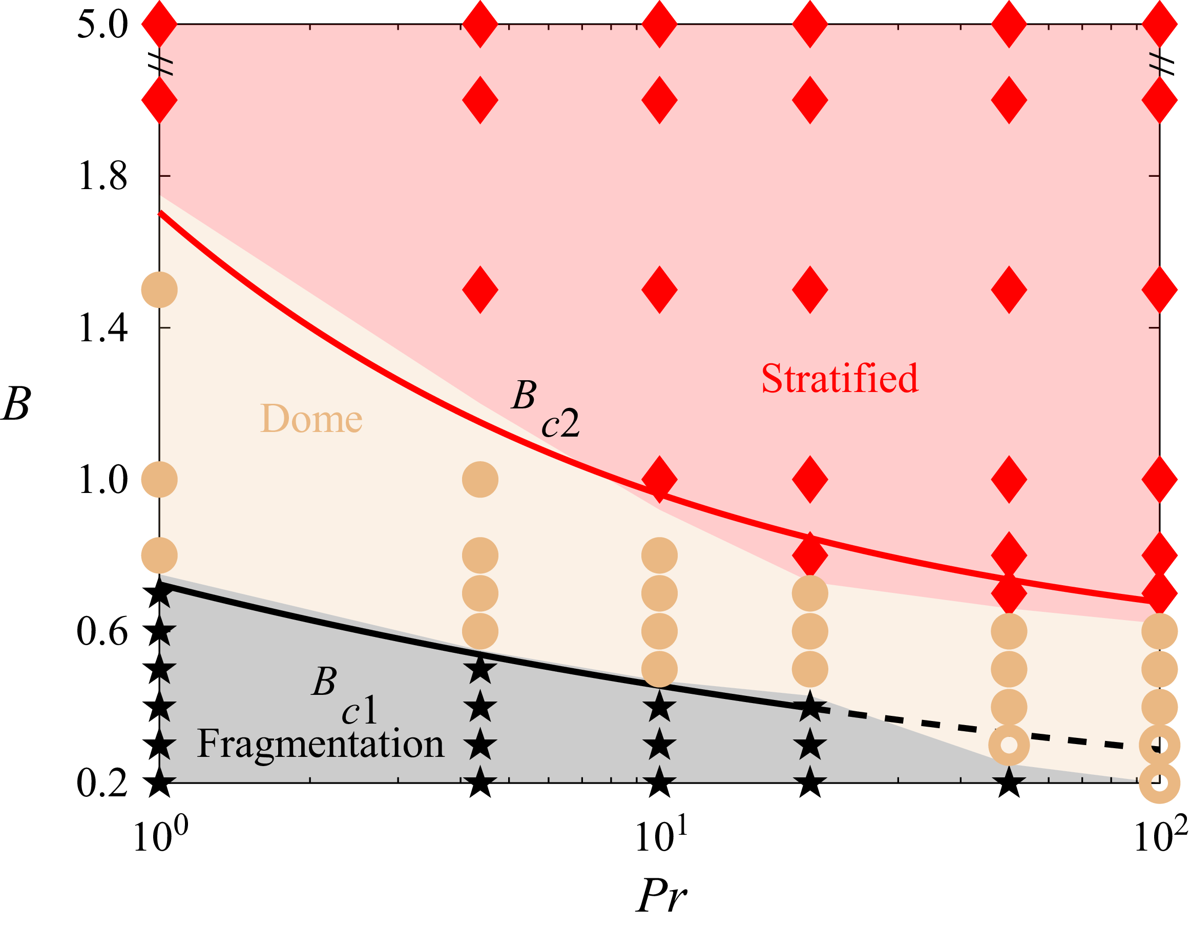
Based on the previously introduced judgment criteria for the different behaviours of the interface, figure 5 plots the phase diagram of the parameter space
 $(B,\textit{Pr})$
, revealing when and what kind of interfacial behaviours will occur. We determined the interfacial fragmentation by the droplet numbers
 $N_{droplets}\gt 0$
(shown in figure 2
e), and dome/superswell by the difference between the highest and lowest interfacial positions being greater than
 $0.1H$
. It can be seen that the system has two critical values
 $B_{c1}$
,
 $B_{c2}$
. When
 $B$
is higher than the critical value
 $B_{c1}$
, the interface transitions from interfacial fragmentation to dome/superswell, and when
 $B$
is larger than the critical value
 $B_{c2}$
, the interface will transition from dome/superswell to stratified convection. It is worth noting that
 $\textit{Pr}$
significantly affects the critical values
 $B_{c1},B_{c2}$
. A natural question arises here: how can the relationship between
 $B_{c1}, B_{c2}$
and
 $\textit{Pr}$
be predicted theoretically?
Phase diagram for the
 $(B,\textit{Pr})$
parameter space. Black five-pointed stars denote the interface fragmentation regime, solid yellow circles correspond to the dome-forming regime, whereas open yellow circles denote the superswell structures. Red diamonds denote the stratified regime. The black and red lines show the theoretical prediction for the transitions between different regimes. The red line (4.9) shows the critical values of dome-forming and stratified regime at high
 $\textit{Pr}$
, which are in good agreement with numerical results. The black line (4.4) shows the critical values for interfacial fragmentation and dome-forming at low
 $\textit{Pr}$
, which match the numerical results for
 $\textit{Pr}\lt 10$
. For
 $\textit{Pr}\gt 50$
, the interface is only stratified or deformed.

To answer this question, we analyse the change in critical values from the momentum equation, where the ratio between the magnitudes of the inertial and viscous forces is as follows:
 \begin{equation} \frac {\boldsymbol{u}\boldsymbol{\cdot }\boldsymbol{\nabla }\boldsymbol{u}}{\nu {\nabla} ^2\boldsymbol{u}}\sim \textit{Ra}^{1/2}\textit{Pr}^{-1/2}, \end{equation}
where we use the free-fall velocity as the characteristic velocity and the domain height as the characteristic length. In this study, we only consider the influence of
 $\textit{Pr}$
, i.e.
 $\textit{Ra}$
is fixed. When
 $\textit{Pr}$
is low, the inertial force of the fluid dominates, thus the inertial force causes the interfacial fragmentation, whereas at this time, the density difference inhibits the interface from breaking up. Ignoring the viscous force of the fluid, the interface breaking up is controlled by the balance between compositional buoyancy and inertial forces. Since the time scale of interfacial fragmentation is small, we ignore the temperature change due to thermal diffusion as well as thermal convection, so the force balance form of the momentum equation can be written as follows:
 \begin{equation} \frac {U^2}{s}\sim \frac {\Delta \rho g}{\rho } , \end{equation}
where
 $U=\sqrt {\alpha \Delta TgH}$
is the free-fall velocity and
 $s$
is the characteristic length of the problem at low
 $\textit{Pr}$
. In the case of the interfacial fragmentation regime, the characteristic length of the system is the characteristic scale of the droplet fragmentation to form a bubble, and we use the Hinze length scale to compute the characteristic scale of the bubble, i.e.
 $s\sim s_{\textit{Hinze}}$
. Based on (3.1), combined with (3.2) and (4.2), we can obtain
 \begin{equation} B_{c1}\sim \textit{Ra}^{-1/5}\textit{Pr}^{-1/5}(\textit{Nu}-1)^{2/5}\textit{We}^{3/5}. \end{equation}
In our computational set-up,
 $\textit{Ra}$
and
 $\textit{We}$
are kept constant. According to the Grossmann–Lohse theory for single-phase Rayleigh–Bénard convection,
 $\textit{Nu}$
is insensitive to
 $\textit{Pr}$
in the regime of
 $\textit{Ra} = 10^7$
and
 $1 \leqslant \textit{Pr} \leqslant 100$
(Stevens et al. Reference Stevens, Van Der Poel, Grossmann and Lohse2013). Consequently, the variation of
 $\textit{Nu}$
has a secondary effect on the predicted regime transitions compared with the dominant influence of
 $\textit{Pr}$
. Thus, for the theoretical derivation of the regime boundaries in (4.3), we approximate
 $\textit{Nu}$
as a constant. Thereby, the equation for the critical value of the interfacial fragmentation can be further simplified as
 \begin{equation} B_{c1}\sim \textit{Pr}^{-1/5}. \end{equation}
When
 $B$
is smaller than the critical value
 $B_{c2}$
, the system changes from stratified convection to the dome-forming regime. For a stratified convection, the interface fluctuation is restricted by the compositional buoyancy force. Thus, in the high-
 $\textit{Pr}$
limit (
 $\textit{Pr} \to \infty$
), where inertial effects vanish, the critical stable state is governed by a pure balance between the compositional buoyancy and the thermal buoyancy:
 \begin{equation} \Delta \rho g \sim \rho \alpha \delta T g, \end{equation}
where
 $\delta T$
is the temperature difference driving the convection within the lower layer. Because the two fluids share identical thermal properties, the system is thermally symmetric, allowing us to focus on the lower layer for convenience. The mean interfacial temperature stabilises exactly at the average of the top and bottom plate temperatures. Consequently, the temperature difference across the lower layer is
 $\delta T = 0.5 \Delta T$
. This is consistent with our numerical simulations shown in figure 4(b), where the dimensionless interfacial temperature is exactly 0.5. Therefore, we obtain the asymptotic limit:
 \begin{equation} B_{c2}(\textit{Pr} \to \infty ) = 0.5. \end{equation}
For a finite
 $\textit{Pr}$
, the inertial force also contributes to the interfacial deformation. The force balance is thus modified to
 \begin{equation} \Delta \rho g \sim \rho \alpha \delta T g + \rho \frac {U^2}{\delta _u}, \end{equation}
where
 $\delta _u$
is the velocity boundary layer thickness. According to the Grossmann–Lohse theory,
 $\delta _u$
scales as
 $\delta _u / H \sim \textit{Ra}^{-1/4}\textit{Pr}^{5/12}$
for
 $\textit{Pr} \geqslant 1$
(Grossmann & Lohse Reference Grossmann and Lohse2001). Substituting the scaling of
 $\delta _u$
into (4.7) yields
 \begin{equation} (B_{c2}-0.5)\sim \textit{Ra}^{-1/4}\textit{Pr}^{-5/12}. \end{equation}
This relation demonstrates that
 $B_{c2}$
converges to the static balance limit of 0.5 as
 $\textit{Pr} \to \infty$
. With the Rayleigh number fixed at
 $\textit{Ra}=10^7$
, the scaling law reduces to
 \begin{equation} (B_{c2} - 0.5) \sim \textit{Pr}^{-5/12}. \end{equation}
This theoretical prediction qualitatively agrees with previous experimental observations for
 $B_{c2}(\textit{Pr} \to \infty ) = 0.35-0.55$
(Davaille Reference Davaille1999a
) and the inertial force introduces a
 $\textit{Pr}^{-5/12}$
correction at a finite
 $\textit{Pr}$
. As shown in figure 5, the red solid line and the black solid line are the results of the theoretical prediction, and it can be seen that the results are well fitted under different
 $\textit{Pr}$
ranges; thus, also indicating the correct theoretical analysis. Notably, at
 $\textit{Pr} \gt 20$
, the theoretical scaling
 $B_{c1}$
also effectively captures the critical boundary for superswell formation, suggesting a consistent physical scaling beyond the fragmentation regime.
5. Conclusions
In this study, a two-layer Rayleigh–Bénard thermal convection system is simulated using direct numerical simulation combined with the phase-field method to investigate the formation mechanisms of superswells and domes, specifically focusing on the roles of
 $\textit{Pr}$
and
 $B$
. Our findings reveal three distinct regimes of interfacial behaviour. At high
 $B$
, where the compositional buoyancy dominates, the system exhibits stratified convection, characterised by a stable interface. For low
 $\textit{Pr}$
and
 $B$
, an inertial–thermal buoyant balance leads to interfacial fragmentation, which can be well predicted by Kolmogorov–Hinze theory. Crucially, as
 $\textit{Pr}$
increases, the influence of inertial forces diminishes, weakening interface breakup and promoting the dome-forming regime.
The focus of this study is the formation of domes and superswells, observed at high
 $\textit{Pr}$
and low
 $B$
. Specifically, at
 $B\lt 0.35$
, a mushroom-like superswell structure forms when rising thermal plumes from the heated lower boundary collide with the upper plate, spreading horizontally. In contrast, for
 $B\gt 0.35$
, the interface deforms into periodic dome structures, where thermal plumes fall midstream without significant horizontal spreading, due to stronger stabilising chemical stratification. Our 3-D simulations corroborate these 2-D observations, showing similar stratified flow, fragmented droplet structures and superswells formation. While 3-D yields slightly higher
 $\textit{Nu}$
than 2-D, the morphological boundaries for the different flow regimes remain consistent within the stated
 $B$
ranges.
We developed a theoretical phase diagram that successfully predicts the transitions between these interfacial behaviours in the
 $(\textit{Pr},B)$
parameter space. For small
 $\textit{Pr}$
, interfacial fragmentation is controlled by the equilibrium between compositional buoyancy and inertial forces. The transition from the stratified to dome-forming regime is governed by a balance among compositional buoyancy, thermal buoyancy and the inertial force by incorporating the finite
 $\textit{Pr}$
effects. We show that
 $B_{c1}\sim \textit{Pr}^{-1/5}$
,
 $(B_{c2}-0.5)\sim \textit{Pr}^{-5/12}$
, and these scalings are in good agreement with the simulation results. In conclusion, this study provides a comprehensive understanding of how
 $\textit{Pr}$
and
 $B$
influence the formation of superswells and domes, along with other interfacial transitions in layered turbulent convection systems, offering framework for predicting interfacial morphology in multiphase systems driven by thermal convection.
Acknowledgements
The authors thank the HPC systems of Max Planck Computing and Data Facility (MPCDF) for the allocation of computational time. The authors also gratefully acknowledge the Gauss Centre for Supercomputing e.V. for providing computing time on the GCS Supercomputers SuperMUC-NG at Leibniz Supercomputing Centre and JUWELS at Jülich Supercomputing Centre (JSC).
Funding
Y.W., H.L. and L.Z. were supported by the Natural Science Foundation of China (Grant Nos. 12388101, 12532011 and 12472224). X.Z. was supported by the Max Planck Society, the German Research Foundation (DFG Grants 521319293, 540422505 and 550262949) and the Daimler and Benz Foundation. L.Z. was supported by a Humboldt Research Fellowship for Experienced Researchers.
Declaration of interests
Authors declare that they have no competing interests.
Author contributions
X.Z. and L.Z. designed the research. Y.W. and H.L. conducted the numerical experiments and analysed the data. All the authors discussed the results and wrote the manuscript.
Appendix A. Droplet detection algorithm
In our simulations, a phase-field variable,
 $C$
, distinguishes between the liquid and gas phases, with
 $C=1$
representing liquid and
 $C=0$
representing gas. The interface between these two phases is thus defined by the
 $C=0.5$
isocontour. We use the MATLAB contour function for this purpose, which efficiently identifies and extracts the coordinates of these isocontours. The algorithm then automatically parses the resulting data structure to count all these individual contours. To handle droplets that cross the periodic boundaries of the simulation domain, a boundary detection is implemented. When a droplet’s contour is found to touch a domain boundary, it is identified as part of a larger droplet that spans the boundary. These split contours on opposing sides of the domain are then effectively re-joined and counted as a single, unified droplet, ensuring an accurate count of all droplets within the system.
The smallest detectable droplet size is implicitly determined by the simulation’s grid resolution. The phase-field method is a diffusive interface approach, requiring at least three grid cells to accurately resolve the interface boundary in our simulations. For a closed contour to be successfully traced, a droplet must be large enough to contain and resolve the interface across its entire diameter. In our 2-D simulation, this necessitates a droplet of at least
 $6\times 6$
grid cells to allow for the formation of a complete and closed loop. This minimum size corresponds to a droplet with a diameter of at least
 $0.0052H$
, where
 $H$
is the domain height.
Comparison of 2-D and 3-D simulations. (a, b) Cross-sections of the 3-D case (
 $\textit{Pr}=50, B=0.3$
) along
 $x=2.5$
and
 $z=2$
, respectively. (c) Comparison of the average temperature profiles. The red lines represent the results for
 $B=5$
and the black lines represent
 $B=0.3$
. Solid lines denote the 3-D simulations, while dashed lines represent the 2-D simulations.

Appendix B. Comparison between 2-D and 3-D simulations
Figure 6 provides a comparative analysis of 2-D and 3-D simulation results. Figures 6(a) and 6(b), which show cross-sections of the 3-D case (
 $\textit{Pr}=50, B=0.3$
) at
 $x=2.5$
and
 $z=2$
, reveal that both the 3-D and 2-D models effectively capture the characteristic superswell structure. Furthermore, a comparison of the average temperature profiles in figure 6(c) provides additional insight by comparing the average temperature profiles. The first comparison is the alignment of the red temperature profiles for
 $B=5$
, indicating strong agreement between the two systems. For the black temperature profiles for
 $B=0.3$
, the 3-D system displays more uniform mixing than the 2-D system. Despite these differences, both systems develop isothermal regions at
 $y=0.5$
, with temperature profiles reminiscent of single-phase flow.
Table 1 compares the Nusselt number (
 $Nu$
) values under different parameters for both 2-D and 3-D simulations. The results are relatively consistent, with the 3-D values being slightly higher than the 2-D values.
This table presents
 $Nu$
of 2-D and 3-D simulations for
 $\textit{Pr}=50$
with different
 $B$
.

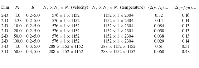
Summary of parameters and grid resolution for
 $\textit{Ra} = 10^7$
and
 $We = 10^3$
.
 $\Delta y_u$
and
 $\Delta y_{\theta }$
denote the vertical grid spacing for the velocity and temperature meshes.

Appendix C. Summary of numerical simulations
Table 2 summarises the numerical parameters and resolution requirements for the DNS cases conducted at
 $\textit{Ra} = 10^7$
and
 $We = 10^3$
. Given the wide range of Pr(
 $1 \leqslant Pr \leqslant 100$
), the velocity field is computed on a
 $576 \times 1152$
grid, while a finer
 $1152 \times 2304$
grid is used for the temperature field to capture the increasingly sharp thermal gradients at high
 $\textit{Pr}$
. The grid spacing is verified against the Kolmogorov scale (
 $\eta$
) and the Batchelor scale (
 $\eta _B$
). To verify the grid resolution, these scales are computed directly from the dimensionless turbulent energy dissipation rate
 $\epsilon$
obtained from the DNS velocity fields. To ensure a conservative estimate of the smallest flow structures,
 $\epsilon _{\textit{max}}$
is determined by first averaging the local dissipation rate over time and the homogeneous horizontal direction, and then extracting the maximum value along the vertical direction. These dimensionless scales are evaluated as
 \begin{equation} \frac {\eta }{H}=\left (\frac {Pr}{Ra \epsilon _{\textit{max}}}\right )^{1/4}, \end{equation}
 \begin{equation} \frac {\eta _B}{H}=\frac {\eta }{H}\textit{Pr}^{-1/2}=\left (\frac {1}{Ra Pr \epsilon _{\textit{max}}}\right )^{1/4}. \end{equation}
As summarised in table 2, the adequacy of the spatial resolution is quantified by the maximum ratios
 $(\Delta y_u/\eta )_{max }$
and
 $(\Delta y_{\theta }/\eta _B)_{max }$
for the velocity and temperature fields, respectively. For each fixed
 $\textit{Pr}$
, these maximum values are extracted across all corresponding
 $B$
. Across all simulations, these conservative ratios remain below unity, confirming that the smallest dissipative structures are fully resolved. Furthermore, all cases were integrated up to a total dimensionless time of
 $t=600$
to guarantee a statistically stationary, fully developed flow state.









 Open access

