Implications
In genetic evaluation models, genetic groups are used to better account for differences in the genetic level between animals without pedigree, also called founders. Usual definition criteria for genetic groups are birth year, country of origin and sex of founders. In the case of a heterogeneous beef cattle population, we showed that a finer group definition, which also accounts for the artificial insemination rate and region of the birth herd of founders, is important to assess genetic disparities in the founder population. This improves both the quality of adjustment to data of the evaluation model and the ranking of candidates for selection.
Introduction
In beef cattle populations, breeding objectives can differ according to the large variety of production systems across and within breeds. In France, regions are characterized by different beef cattle production systems, which correspond to different breeding objectives. The relative use of artificial insemination (AI) and natural service (NS) may also greatly vary between herds and regions. These different selection and mating practices may generate genetic heterogeneity in the population of any beef cattle population. Ignoring such heterogeneities in the base population may lead to biased prediction of breeding values (BV) and suboptimal choice of breeding stock. The best linear unbiased prediction (BLUP) of BV is truly unbiased when pedigree and data information are exhaustive to trace back to an unselected and unbred population. Only under such an assumption, it makes sense to use a genetic evaluation model with a unique base population whose BV are normally distributed with a zero mean and a variance equal to twice the Mendelian variance (Henderson, Reference Henderson1973). However, this assumption is violated in practical evaluation of a population undergoing selection for decades. To account for the genetic trend and heterogeneity in the base population, unknown parent groups (UPG) may be defined. As suggested by Westell et al. (Reference Westell, Quaas and Van Vleck1988) and Banos et al. (Reference Banos, Schaeffer and Burnside1991), group definition is often based on birth year, country of origin and selection path. However, for large beef cattle populations, those criteria may not be fully sufficient to define UPG. As far as we know, no methodology has been proposed to define relevant UPG at the national level for large heterogeneous populations. This study presents a procedure to define UPG for beef cattle genetic evaluations. The method is based on the characterization of bull usage patterns across herds.
Material and methods
Data
The French Charolais cattle were analyzed as a case study in order to define genetic groups in a large beef cattle population. This breed has had great expansion in France since the 1960s, potentially creating genetic heterogeneous subpopulations across French regions. Data were extracted from the French national cattle database, which is used for on-farm genetic evaluations of weaning traits. The analyzed population included 2 936 732 calves sired by 98 848 bulls. Animals were born between 1972 and 2006 in 8157 herds having at least five calves recorded at weaning per year.
Two traits were analyzed: muscle score at weaning (MS, mean = 63.0 points, s.d. = 11.9 points) and skeleton score at weaning (SS, mean = 64.3 points, s.d. = 9.7 points). Both of them are scored from the visual appraisal over a 100-point scale. The MS is a sum of scores for five different items in order to assess the calf muscularity (muscle thickness and width) of its shoulders, back and rump. The SS is a sum of scores for five other items to assess the calf skeletal frame (bone thickness and length) of its back, pelvis and canon bone. Statistical analyses were carried out with version 9.1 of the SAS software (SAS Institute Inc., Cary, NC, USA, 2004). The ASREML software (Gilmour et al., Reference Gilmour, Gogel, Cullis, Welham and Thompson2002) was used to estimate variance components and log-likelihoods of models. The Genekit software (V. Ducrocq, personal communication) was used to perform BLUP evaluations.
Identification of genetic heterogeneity sources in the population
Three factors, which could cause genetic heterogeneity in the population, were identified: time, AI rate and region of herds.
Characterization of time periods
Since the beginning of the French beef cattle recording system in 1972, important political or technical events have led to strong changes in French beef cattle breeding schemes over time. Four periods were considered to analyze the data. The first one occurred from 1972 to the setting up of milk quotas in 1983. This latter event boosted the countrywide expansion of the Charolais breed during the second period running from 1983 to 1991. The third time period (1992 to 1998) started with the setting up of the BLUP animal model methodology for on-farm genetic evaluations. The last time period (1999 to 2006) was characterized by an increase in the unknown parent rate. Indeed, quite a lot of new herds entered the performance recording system at this period and more stringent validation procedures of genealogies were set up in 1999 (Journaux et al., Reference Journaux, Berrechet and Ledos2006). These phenomena led to an increase in the annual rate of unknown parents from about 2% to 5%.
Characterization of the relative use of AI and NS
In France, about one-third of Charolais calves are procreated by AI in herds with performance recording (Bouquet et al., Reference Bouquet, Renand and Phocas2009). To account for genetic differences between AI and NS bulls due to different selection intensities, herds in each region were separated according to the rate of calves sired by AI bulls: herds with an AI rate below 50% (NS herds) and above or equal to 50% (AI herds).
Characterization of regional subpopulations
Given the great variety of production systems in France, there was evidence of regional genetic heterogeneity in the Charolais population (Bougler et al., Reference Bougler, Le Liboux, Hocde and Vissac1973). Unfortunately, no information about production systems was recorded. Several regions were therefore identified using data available for genetic evaluations. An approach combining a principal component analysis (PCA) and a clustering algorithm was chosen to automate the classification of administrative departments into production regions.
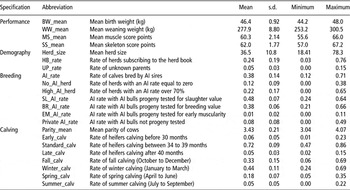
Normalized PCA was carried out to synthesize 22 parameters that were means of diverse Charolais herd characteristics per administrative department. Parameters are listed in Table 1 and are related to herd performance at birth and weaning of calves, herd demography, breeding and calving practices. Departments were then aggregated in regions presenting common features using a Ward hierarchical ascendant clustering (HAC) algorithm on the PCA results. This approach combining PCA and Ward HAC was applied to the four time periods, described in the previous paragraph, in order to detect temporal evolutions of regional beef cattle production and breeding practices. Within a time period, analyses were carried out only on departments, which counted at least five herds and 1000 animals to avoid inconsistent classification due to insufficient number of records. For instance, the last period included 59 departments, representing 1 274 304 animals born in 4514 herds. The automatic clustering of departments allowed identifying four large regions with similar calf performance and breeding practices. To describe more exhaustively all potential regional genetic heterogeneities in the population, a finer definition of regions had been adopted on the basis of three ad hoc division criteria. The first criterion was to form regions with at least 100 000 registered animals. The second one was to consider additional information on the selection history of the French Charolais breed related by Bougler et al. (Reference Bougler, Le Liboux, Hocde and Vissac1973) and experts of the Charolais breed association. The third one was to constitute regions composed of close departments to conserve a geographical consistency.
Means, standard deviations and extrema of 22 Charolais herd parameters used in the PCA of average Charolais herd records from 59 French departments in the period 1999 to 2006

PCA = principal component analysis; AI = artificial insemination.
Definition of UPG
The definition of UPG aims at capturing genetic differences existing between genetically homogenous subpopulations of unknown parents, which were used in the same period (Robinson, Reference Robinson1986; Westell et al., Reference Westell, Quaas and Van Vleck1988). However, a too fine definition of UPG is not desirable because a sufficient number of animals in each group is necessary to get precise estimates of UPG effects and to avoid confounding with other fixed effects in the model (Quaas, Reference Quaas1988). In practice, Interbull guidelines for international evaluation of dairy traits recommend a minimum of 10 to 20 bulls per group (Interbull, 2001). Although the introduction of UPG in a genetic evaluation model may reduce bias, it also increases prediction error variance of BV due to the higher number of parameters in the statistical model. If differences between UPG estimates are not large enough, Kennedy (Reference Kennedy1981) proved that a model without UPG could be preferred to a model with groups for minimizing the mean square error.
To reduce the number of UPG defined for the beef cattle evaluation in a relevant way, we postulated that two herds with a similar supply of identified bulls should have used unknown parents with similar genetic levels. These unknown parents were therefore supposed to be drawn for the same genetic group. The supplying strategy in cows was not considered to define UPG because cow flows across herds were negligible in comparison to bull flows. Moreover, differences between BV of cows were expected to be smaller than the ones between BV of bulls, due to the higher selection intensity on the sire selection path.
Within each time period, founders born in herds from different combinations of ‘AI rate × region’ were assigned to a same UPG when their birth herds had used at least 70% of bulls with similar genetic levels and origins. The origin of a NS bull was defined by the region and the degree of specialization in breeding of the birth herd. Breeding herds were split into two categories: specialized herds, which sold at least five males for breeding each year and occasional breeders, which sold less than five bulls per year to other herds carrying out performance recording. A third category was defined for AI bulls because they were submitted to higher selection intensity than NS bulls.
Hence, within each time period, sire origin effects were estimated for each trait (MS and SS) as fixed effects in a linear model including also the birth region, herd, birth year and sex of the recorded calves with known sires. These effects provided an estimation of the mean genetic level of AI and NS bulls according to their origin. Then, for each trait, the mean genetic level of sires used in herds of each combination of ‘AI rate × region’ was calculated. To do so, estimates of sire origin were weighted by their contributions to the total number of progeny of those herds. In practice, differences in estimated genetic level of identified sires had to be lower than 20% of genetic standard deviation (σ g) for both traits to consider that founders born in different herd categories belonged to the same UPG. This arbitrary value was fixed as an ad hoc limit corresponding to the minimum genetic difference below which Phocas and Laloë (Reference Phocas and Laloë2004a) considered that including groups in the genetic evaluation of a progeny testing scheme will be counterproductive in terms of selection response and average mean square error of BV.
In the construction of the genealogy file, three categories of animals had to be considered to define UPG: bulls, cows and calves not yet used for reproduction. All calves belonging to the evaluated population and not yet used for reproduction had systematically their dam, birth date and herd known. When a bull or a cow had an unknown parent, this parent was replaced with the UPG corresponding to the criteria relative to the year, the region and the AI rate of the herd in which it was used. When one of the criteria was missing, it was deducted according to the following rules. In case of a founder bull, it was determined if it was used by AI. Such information was available in a database, which listed all bulls used by AI since the 1960s. The birth year of a founder was derived from the average birth year of its offspring and a generation interval of 8 years for AI bulls, 4 years for NS bulls and 5 years for cows. As birth dates of a founder’s offspring could be unknown, an iterative procedure was used to predict the birth year of all ancestors from the controlled calf population to the founders. Genetic groups were cross-classified by sex to account for bull and cow selection paths. The same UPG definition criteria were adopted to define bull and cow groups. A cross-classification with the sex of the unknown parent would have accounted for the usual four selection paths, but it would have induced confounding effects between sire and dam UPG because both parents were unknown in 92% of cases of incomplete pedigree. Eventually, when the birth herd of a founder was unknown, the region was derived from the national identification number of the founder, which contains the number of the birth department, and the AI rate was assumed to be below 50% because NS is the main reproductive mode in the French Charolais cattle population (Bouquet et al., Reference Bouquet, Renand and Phocas2009).
Estimation of UPG effects and BV
We proceeded to a genetic evaluation without and with genetic groups to evaluate the impact of introducing such groups in the model. Without UPG, the following mixed linear model was considered for each trait:

where y is the vector of observations, a is the age at scoring taken into account as a covariate, α is the corresponding regression coefficient, b is a vector of fixed effects, u, c and e are random vectors representing BV, permanent environmental (dam) and residual effects, respectively. X, Z and W are the corresponding incidence matrices.
The b vector considered the fixed effects of status at scoring, particular treatments before weaning, birth season, age of dam and contemporary group. Status at scoring counted three levels: weaned, just weaned and not weaned calves. Particular treatments before weaning also corresponded to three levels: no treatment, favorable and unfavorable treatments. The 10 classes of the birth season effect corresponded to each single month from October to May and to the association of June and July on the one hand and August and September on the other hand. Classes of dam age had 10 levels as follows: classes 1, 2, 3, 4, 5 corresponded to primiparous dams with age at first calving, respectively, strictly lower than 27 months, between 27 and 30 months, 31 and 33 months, 34 and 39 months and, finally, over 39 months. Classes 6, 7, 8, 9 and 10 corresponded to multiparous cows whose age belonged, respectively, to the interval 34 to 39 months, 40 to 52 months, 53 to 65 months, 66 to 126 months and over 126 months. Contemporary groups were defined as combinations of birth herd, birth year, management group and sex of the calves. The random vector of BV included either sire or animal genetic effects assumed to be normally distributed in a sire and animal model, respectively. Genetic relationships among sires, or among animals, took into account up to three generations of ancestors, including 195 238 and 3 310 940 animals, respectively. Dam permanent environmental effects were taken into account but no maternal genetic effects were considered due to small maternal heritabilities for SS and MS (Phocas and Laloë, Reference Phocas and Laloë2004b).
In the model with UPG, genetic groups were estimated as fixed effects according to Westell et al. (Reference Westell, Quaas and Van Vleck1988). The vector of total BV û is predicted as  where
 is a vector containing the UPG effects, Q is a matrix whose rows represent the gene proportion of the recorded animal originating from each UPG and
 is the vector of BV within UPG effects. Keeping the same matrix notations, the mixed model for y can be written as:

In a sire model, the BV of a sire ( ) is equal to half of its additive genetic value, which would be predicted in an animal model (
 ). The UPG estimates in a sire model are therefore equal to half of UPG effects estimated in an animal model.
Variance components were estimated under each sire model (1) and (2) on 10 data samples of 300 herds. Whatever the model, average phenotypic variances were estimated to 62.8 points2 and 97.4 points2, respectively, for SS and MS. The corresponding estimates of heritability (h2) were 0.19 and 0.26. The ratio (c2) of permanent environmental variance to phenotypic variance also remained equal to 0.05 and 0.11, respectively, for SS and MS. Therefore, variance components used in the evaluation models of the whole data set were fixed at the herein values.
Validation of the UPG definition
The definition of large and homogenous genetic groups is necessary to ensure that UPG estimates will be accurate and relatively constant between two evaluation runs, avoiding inappropriate re-ranking of animals (De Jong, Reference De Jong2003; Fikse, Reference Fikse2003). The UPG definition will be declared relevant if it is fine enough to model correctly genetic heterogeneity among the founder population but not too fine to get precise and robust UPG estimates. To limit computation requirements, a sire model was used to validate the UPG definition in terms of goodness-of-fit and predictive ability of the model but also significance and robustness of the UPG estimates.
Goodness-of-fit of a model without and with UPG
The goodness-of-fit of models with and without groups was evaluated for genetic evaluation of MS and SS on representative samples of 300 herds (10 replicates). It was not calculated with the Genekit software on the whole population because this software did not display the log-likelihood of the model. Nested models were compared in order to assess the interest of the full model including UPG defined according to the three criteria (time period, herd AI rate and region) to a model corresponding to current industry standard only accounting for the genetic trend in UPG, or to an intermediate model with a UPG definition based on time period and AI rate of herds to account for the AI v. NS sire selection paths. As we were interested in the predictive ability of the models, we chose to compare the goodness-of-fit of models using the Akaike information criteria (AIC; Akaike, Reference Akaike1973). Indeed, the AIC appears to be more appropriate than the likelihood ratio test or the bayesian information criterion to select the best model in a prediction purpose (Ward, Reference Ward2008).
Significance of UPG estimates
To test the significance of differences between pairs of UPG estimates, we used approximated standard errors. They were calculated by directly inverting the coefficient matrix of the left-hand side of BLUP equations for the whole population under a simplified sire model. This simplified model only took into account the sire and the contemporary group effects. In a 2000 herd sample, we checked that approximated standard errors were underestimated only by 2% to 6% compared to standard errors obtained by directly inverting the coefficient matrix of the left-hand side of BLUP equations for the complete model. As standard errors of UPG estimates were slightly underestimated, we considered a stricter threshold significance level (1%) than usual (5%) to compare UPG estimates.
Robustness of the UPG effects
To test the homogeneity and numerical stability of the N genetic groups, UPG were split into two genetic subgroups of equal size and founders of each group were randomly attributed to each subgroup. Genetic evaluation was then carried out with a model accounting for 2N genetic groups in order to estimate all the subgroup effects. This operation was replicated 10 times and means and standard deviations of subgroup effects were derived from the estimates of the 10 replicates.
Results and discussion
Characterization of regional subpopulations with factorial methods
Identification of regions
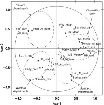
Results of the factorial analyses used to build up regions are presented only for the last time period (1999 to 2006) because they are consistent with those of the preceding time periods. The first principal component of the PCA accounted for about 30% of the total variance existing between French departments. It discriminated departments in the center of France, the originating region of the Charolais breed, from the rest of the departments (Figure 1). The second component of the PCA summarized 18% of the variance and mainly discriminated North Eastern departments from Western and Southern ones. The main characteristics of each region are given in Figure 1, which shows the correlation between each variable and the first two components of the PCA.
Correlation circle of the first two principal components of the principal component analysis with the 22 parameters describing Charolais herds across French departments for the 1999 to 2006 period. Circles in dotted line and italic names indicate the localization of departments on a map of France. Abbreviations of variables are listed in Table 1.

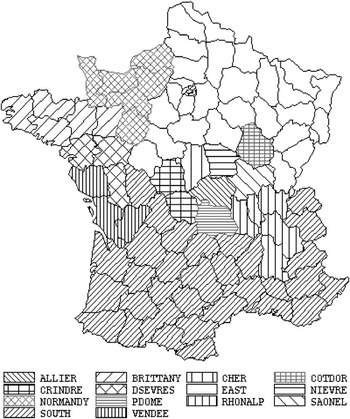
The Ward HAC enabled to automate the aggregation of the 59 departments into four geographically consistent regions. They corresponded to (i) the departments of the center of France, (ii) the Western departments, (iii) the Southern region and eventually (iv) a large set of departments in the North Eastern part of France. These four clusters explained 42% of the total variance, which was rather limited. However, a more detailed automatic clustering would have formed regions with unbalanced population sizes or made up of geographically distant departments. To have a deeper insight into regional heterogeneities, these four clusters were further split into 14 regions (Figure 2).
Representation of the 14 French Charolais breeding regions.

Flows of bulls between regions
Since 1983, flows of NS bulls remained very similar across regions and appeared to be carried out mostly on short distances. Whatever the region considered, more than 50% of the NS bulls were used in their native region. The remaining NS bulls came essentially from herds of the Charolais selection nucleus, which are mainly located in three breeding regions: Allier, Vendée and the association of Saône-et-Loire and Nièvre departments. It was observed that those breeding regions specifically supplied in NS bulls herds located in three distinct areas. Consequently, NS bull flows across the 14 regions could be encompassed within three main breeding areas: the Center Southern breeding area around Allier, the Western breeding area around Vendée and the North Eastern breeding area around Saône-et-Loire and Nièvre. There were very limited (below 13%) exchanges of NS bulls between those breeding areas.
Definition of UPG
Taking into account the four time periods, the 14 regions and the two AI classes could have led to the definition of 112 UPG. To reduce the number of defined UPG for each time period, sire origin effects were estimated in order to gather in the same UPG founders from combinations of ‘AI rate × Region’ exhibiting similar genetic levels (results not shown). Large differences in sire effects were estimated between AI and NS bulls, especially for SS. For this latter trait, average genetic differences between AI and NS bulls reached more than one genetic standard deviation. This highlighted the high selection intensity on AI sires to produce large framed cows with wide pelvises. These results validated the partition of herds according to their AI rate as a good indicator of the selection intensity on the various sire selection paths.
For NS bulls, sire origin estimates were relatively homogenous across birth regions within a breeding area, but quite different across areas. The low genetic mixing between areas contributed to maintaining three distinct subpopulations in the French Charolais cattle population.
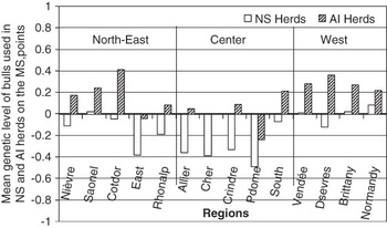
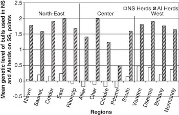
The average genetic levels of sires used in each region are presented for MS and SS in Figures 3 and 4, respectively. They are expressed in contrast to the sire origin estimates for NS bulls bred by specialized breeders from the Nièvre. For both traits, the mean genetic levels of bulls used in NS herds were quite heterogeneous between breeding areas. On the contrary, differences in the mean sire level of NS herds located in regions of a same breeding area were lower than 20% σ g. Consequently, within each time period, three regional UPG (West, Center South and North East) were defined for unknown parents used in NS herds. They correspond to the three breeding areas that encompassed the initial 14 regions. As expected, within a region, the genetic level of sires used in the AI herds was higher than the one of sires used in the NS herds. Some genetic differences were detected between AI herds of various regions, but they were lower than 20% σ g on MS and SS, except for the PDome region. As very few bulls without pedigree were used in AI herds of PDome, hardly one bull per year, and the choice of AI sires was mainly done among a national pool of bulls, a single UPG was defined for AI herds within a given time period, whatever their location in France.
Mean genetic level on the muscle score (MS) of bulls having sired calves born in natural service (NS) herds and in artificial insemination (AI) herds belonging to the 14 French regions between 1999 and 2006.

Mean genetic level on the skeleton score (SS) of bulls having sired calves born in natural service (NS) herds and artificial insemination (AI) herds belonging to the 14 French regions between 1999 and 2006.

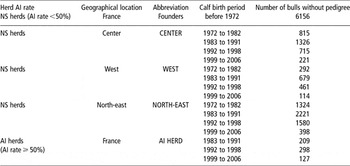
Between 1972 and 1982, since the number of AI herds was negligible, only three regional groups were defined whatever the AI rate of herds. Before the start of the recording system in 1972, a single UPG was defined because most of the animals were located in the originating region of the breed (Bougler et al., Reference Bougler, Le Liboux, Hocde and Vissac1973). Thus, 16 genetic groups were defined groups, as reported in Table 2.
Summary of the defined UPG and the criteria used for their definition

UPG = unknown parent groups; AI = artificial insemination; NS = natural service.
Validation of the UPG definition
Goodness-of-fit of models
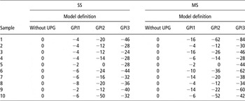
For each of the 10 samples of 300 herd records, the goodness-of-fit estimated in sire models for MS and SS with the 16 UPG herein defined were compared to two other models with more parsimonious UPG definitions and also to a model without genetic groups. Whatever the sample and the trait, the AIC was always lower in the current industry standard model with a group definition based only on time periods (five groups) than in the model without a group. This indicated that the model with genetic groups should be preferred in terms of goodness-of-fit and predictive ability for the complete data set (Table 3). The goodness-of-fit of a model with eight UPG based on time periods and AI rate of herds was compared to the one of the model with the time-based group definition (five groups). For both traits, in nine out of the 10 samples, the AIC clearly indicated that the AI rate of the herds had to be considered in the UPG definition. The full model with 16 UPG was finally compared to a group definition, based on the criteria ‘time period’ and ‘herd AI rate’. Lower AIC were found in nine out of the 10 samples on SS and MS. The regional group definition was also necessary to improve the goodness-of-fit to the data. Thus, it can be concluded that the time period, the AI rate and the breeding area of the herds in which unknown parents were used had to be accounted for in the UPG definition to improve the model fit to data of the French Charolais cattle population.
AIC calculated on MS and SS for models without group and with a UPG definition based on time periods (GPI1), on time periods and AI rate (GPI2) and on time periods, AI rate and regions (GPI3)

AIC = Akaike information criteria; MS = muscle score; SS = skeleton score; UPG = unknown parent groups; AI = artificial insemination.
All criteria are expressed in contrast to the AIC of the model without group.
Estimation of the unknown sire group effects
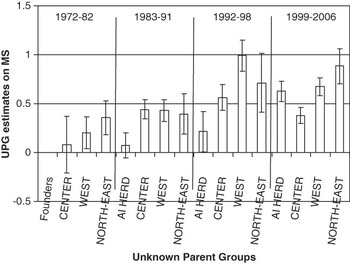
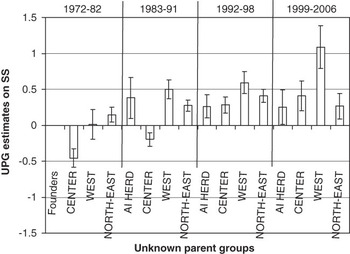
Figures 5 and 6 present the UPG effects estimated in a sire model for MS and SS, respectively. They were converted to an animal model equivalent ( ) and then expressed in σ g units. Whatever the trait, UPG estimates within a breeding area generally increased over time due to the genetic trend in the unknown parent subpopulations. Great regional disparities within a time period were also marked, up to 50% σ g on the last decade, for both traits. This confirmed the AIC results that both the genetic trend and the regionalized breeding strategies were important sources of genetic heterogeneity to take into account for the definition of the genetic groups.
Sire unknown parent groups (UPG) estimates for muscle score (MS), expressed in contrast to the founder UPG estimate and in units of genetic standard deviation and their 99% confidence intervals.

Sire unknown parent groups (UPG) estimates for the skeleton score (SS) expressed in contrast to the founder UPG estimate and in units of genetic standard deviation and their 99% confidence intervals.

Although significant differences were estimated between UPG at a 1% level, those differences could be insufficient in magnitude to effectively recommend their introduction in the evaluation model. Indeed, Phocas and Laloë (Reference Phocas and Laloë2004a) showed that a model without UPG could be preferred to a model with groups in terms of mean square error and selection efficiency when considering the likely genetic trend and the amount of information available for progeny test evaluation of beef cattle.
Robustness of the UPG
Simple rules consisting of randomly dividing UPG into two subgroups of equal size were used to validate the robustness and numerical stability of the defined UPG. The 10 replicate means of subgroup effects of a same UPG were not significantly different from each other and were close to those estimated for the whole UPG (results not shown). Until the 1980s, the 10 replicate standard deviations of subgroup estimates was moderate (<20% σ g), showing that UPG estimates were stable and relied on a homogenous bull population that diffused a lot across herds. Those standard deviations were greater for the following periods, especially for UPG of small size. About 60 bulls directly linked to the smallest subgroups seemed to be insufficient to get stable estimation of UPG effects. By partitioning UPG, we noticed that at least 100 bulls per subgroup were necessary to get stable estimates of UPG, meaning their sampling standard errors were below 20% σ g. This minimal number of bulls is much greater than the Interbull recommendations, probably because Charolais bulls without pedigree have 14 progeny on average for the estimation of their BV, which is much fewer than in dairy cattle populations.
Application of the UPG definition for the animal model used in the French beef evaluation
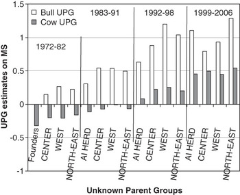
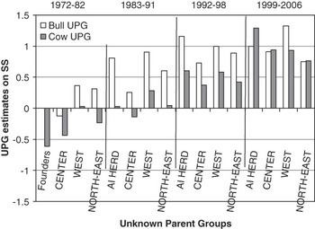
The final aim was to implement a new animal model including relevant UPG for the French on-farm genetic evaluations. A genetic evaluation was therefore carried out under an animal model accounting for UPG using the same definition criteria for bull and cow genetic groups. Bull and cow UPG estimates are presented in Figures 7 and 8 for MS and SS, respectively. They are expressed in contrast to the UPG estimate of the bull founder group. With regard to MS, bull UPG effects were close when comparing estimates from the sire and the animal models. With regard to SS, bull UPG estimates were systematically higher (up to 70% σ g) in the animal model than in the sire model. Indeed, cows kept for breeding are generally highly selected on SS. Their genetic level was observed to be about 30% σ g higher than the one of contemporary animals born in the same year. Therefore, ignoring dams in the sire model tended to increase the contemporary group estimates to the detriment of genetic group effects.
Unknown parent groups (UPG) estimates in the animal model for muscle score (MS), expressed in contrast to the bull founder UPG estimate in units of genetic standard deviation.

Unknown parent groups (UPG) estimates in the animal model for skeleton score (SS), expressed in contrast to the bull founder UPG estimate in units of genetic standard deviation.

Cow UPG effects estimated for SS were also lower by 30% to 50% σ g than bull estimates until the 1990s (Figure 8). However, over the last decade, cow UPG estimates became equivalent or even greater than bull UPG estimates. With regard to MS, cow UPG estimates were lower by about 50% σ g than the ones of bulls because of lower selection intensity for cows (Figure 7). They were also homogenous across breeding areas, whereas bull UPG estimates exhibited differences across areas up to 50% σ g.
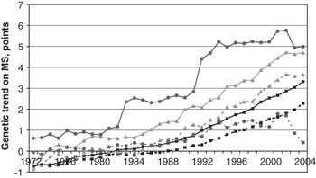
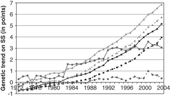
Genetic trends in MS and SS are presented in Figures 9 and 10, respectively, for the whole calf population and for bulls without and with pedigree in models without and with UPG. Genetic trends estimated in the model with groups were expressed in contrast to the effect of the bull founder group. To gain clarity, genetic trends estimated in the model without group were centered so that the mean genetic level of the calf population born in 1972 is the same in both models. As the definition of genetic groups in the evaluation model allowed accounting for differences in genetic levels among unknown parents, a greater genetic trend was estimated both for MS (Figure 9) and SS (Figure 10). For instance, between 1992 and 2004, genetic trends of 2% and 7% σ g per year were estimated in the model without UPG on MS and SS, respectively. These trends reached 3% and 8% σ g per year on MS and SS when calculated in the model with groups. Between 1972 and 1991, genetic trends were lower but the difference in genetic trend between both models remained comparable to the one calculated between 1992 and 2004. As expected, animals with the most affected BV when including UPG in the evaluation model were the ones without pedigree. Comparison of the BV ranking across models indicated that there would be little re-ranking for bulls, especially for elite bulls whose genealogy was well known. On the contrary, large re-ranking would happen for cows without pedigree between the model with UPG and the current model without group.
Genetic trends estimated for the muscle score (MS, σ g = 5.0 points) in an animal model with genetic groups (plain line) and without groups (dotted line) according to calves (▪), bulls with known pedigree (▴) and bulls without pedigree (●).

Genetic trends estimated for the skeleton score (SS, σ g = 3.5 points) in an animal model with genetic groups (plain line) and without groups (dotted line) according to calves (▪), bulls with known pedigree (▴) and bulls without pedigree (●).

As genealogies of AI sires were extensively known, bulls without pedigree were NS bulls, even when they were used in AI herds. As shown in Figures 9 and 10, very different genetic levels were estimated between bulls with and without pedigree. Therefore, it seems that bulls without pedigree are not selected for the same objectives as bulls with pedigree. However, it is consistent that farmers who have a similar supplying strategy in bulls would use bulls without pedigree for the same grounds. In the French Charolais population, evidence supported that bulls without pedigree were mostly ‘back-up’ bulls used to produce calves for slaughtering (high MS wanted) rather than for replacement (high SS wanted). In practice, the postulate led to the definition of bull UPG, which exhibited significant genetic differences between them. The postulate is also clearly relevant to define genetic groups for cows. Actually, a frequent motive of absence of pedigree is the joining of new herds to the recording system. In those herds, parents of animals born before subscription are generally not recognized. As flows of cows across herds are rather limited, the genetic level of cows without pedigree reflects quite well the genetic level of their native herd. Over the last decade, this was confirmed on SS by both a higher mean genetic level of bulls used in AI herds than in NS herds (Figure 4) and a 35% σ g higher cow genetic group estimate in AI herd than in regional NS herd UPG (Figure 8). Similarly, differences in genetic level estimated on MS were small between bulls used in AI and NS herds across regions (Figure 3), which was consistent with the homogenous cow UPG effects estimated within a given time period (Figure 7).
To conclude, bull usage patterns observed across herds are a relevant source of information to define UPG for a beef cattle genetic evaluation. The method presented in this study permitted to identify relevant UPG that exhibited large genetic differences across time periods and regions. This methodology, as well as the three criteria – time, AI rate and breeding area – proposed to define UPG for the French Charolais population, may be of general interest for any large beef cattle population undergoing selection.
Acknowledgements
Authors would like to acknowledge French beef cattle breeding associations and companies for their collaboration and financial support to this work.