1 Introduction
The study of fluid–structure interactions with vegetation has a wide range of industrial and environmental applications, including flood control, environmental conservation and energy production. However, there are a number of challenges in modelling such flows, in particular due to the fact that the vegetation both affects and is affected by the flow. The focus of this work is to develop compact mathematical models that describe flows through submerged vegetated regions and their resultant instabilities. In particular, we predict the critical parameters in different regimes for instabilities which resemble monami – the synchronous waving of vegetation.
1.1 Flow through aquatic vegetation
Climate change is increasing the frequency and severity of hydrological disasters. While there are many infrastructural approaches to flow management, there is also an emerging interest in utilising aquatic vegetation, as it is part of the natural habitat helping to sustain our ecosystems. Compared to artificial measures, aquatic vegetation has the promising ability to adapt to the local environment, grow and multiply as a canopy, even after destructive events (Morris et al. Reference Morris, Konlechner, Ghisalberti and Swearer2018). On the other hand, flows through vegetation are challenging to model due to the complex interactions which take place. Thus the efficiency of aquatic vegetation in protecting coastal regions, and the physical mechanisms involved, are yet to be fully understood (Marion et al. Reference Marion, Nikora, Puijalon, Bouma, Koll, Ballio, Tait, Zaramella, Sukhodolov and O’Hare2014).
Aquatic vegetation is typically flexible and streamlined, which allows it to passively reconfigure, reducing the fluid load (Vogel Reference Vogel1994). In addition to its deformable nature, it can also have a complex geometry, with components that can have length scales that differ by several orders of magnitude. Finally, as distinct from terrestrial flows, submerged vegetation has a typical height comparable in magnitude to the water depth in order to photosynthesise (Marion et al. Reference Marion, Nikora, Puijalon, Bouma, Koll, Ballio, Tait, Zaramella, Sukhodolov and O’Hare2014). As a result, a significant proportion of the flow is obstructed by the canopy – a community of vegetation.
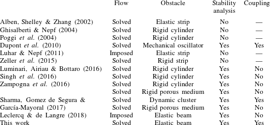
Modelling approaches of a selection of previous work on flow through a single or a collection of obstacles. The ‘Coupling’ category states whether the stability analysis takes into account for perturbations of both the flow and the obstacles.

There are numerous modelling challenges in capturing the macro- and micro-scale properties of the system, primarily relating to the feedback mechanism between flow and vegetation. In a complete dynamic model, the fluid will apply a load on each vegetative structure, which causes a resultant deformation and this, in turn, must affect the flow. Thus, in general, it appears that the fluid flow must be solved simultaneously with the configuration of each structure. These challenges have demanded sophisticated studies; see e.g. experimental works by Dunn, Lopez & García (Reference Dunn, Lopez and García1996), Ghisalberti & Nepf (Reference Ghisalberti and Nepf2004), Hu et al. (Reference Hu, Suzuki, Zitman, Uittewaal and Stive2014) and Mandel et al. (Reference Mandel, Gakhar, Chung, Rosenzweig and Koseff2019) and numerical works by Mattis (Reference Mattis2013), Zeller et al. (Reference Zeller, Zarama, Weitzman and Koseff2015), Sundin & Bagheri (Reference Sundin and Bagheri2019) and Sharma & García-Mayoral (Reference Sharma and García-Mayoral2020).
In this work we explore simpler mathematical models that are able to capture a number of the key physical features of more complicated formulations or experiments. With regard to the development of simplified models, the vast majority of previous work has fallen in two categories: either models of flow over a specified set of rigid obstacles (see e.g. Ghisalberti & Nepf (Reference Ghisalberti and Nepf2004)); or models where plant deformation can occur, but only under a known imposed flow (see e.g. Luhar & Nepf (Reference Luhar and Nepf2011)). There have been fewer models that emphasise the coupling between deformation and flow. We highlight, in particular, the work of Alben et al. (Reference Alben, Shelley and Zhang2002) on flow past a single elastic strip in two dimensions and Dupont et al. (Reference Dupont, Gosselin, Py, de Langre, Hemon and Brunet2010) on flow past an array of rigid straight elements that are free to tilt. A summary of previous work and their key features are presented in table 1.
1.2 Instabilities in aquatic vegetation
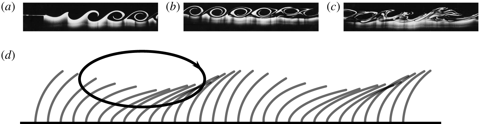
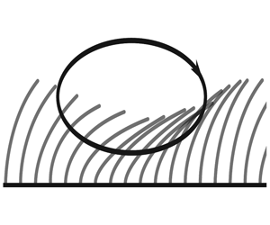
Part of the emerging interest in instabilities of flow through a canopy is sparked by a phenomenon known as monami (see the schematic in figure 1) – the progressive, synchronous oscillation of aquatic vegetation (Nepf Reference Nepf2012). Honami, its counterpart in terrestrial flows, is readily observable in daily life when wind blows across a patch of grass or a crop field (de Langre Reference de Langre2008). Only relatively recently has the phenomenon of honami been explained by Raupach, Finnigan & Brunet (Reference Raupach, Finnigan and Brunet1996), pointing out that such instabilities arise due to a shearing mechanism that resembles the Kelvin–Helmholtz instability on free mixing layers at the top of the canopy. Once the shear exceeds a threshold, waves develop in the flow which evolve into vortices over time (cf. top insets of figure 1). The argument that such instabilities are distinct from boundary-layer instabilities is supported by comparing the statistics of turbulent kinetic energy in experiments (Finnigan Reference Finnigan2000; Poggi et al. Reference Poggi, Porporato, Ridolfi, Albertson and Katul2004).
Many studies have applied similar explanations to the development of monami by analysing the stability of steady states in their respective models (cf. table 1). In particular, Singh et al. (Reference Singh, Bandi, Mahadevan and Mandre2016) established the dependence between viscous effects and flow instabilities by analysing flows through an array of rigid beams.
Schematic diagram of monami – the synchronous oscillation of aquatic plants. The grey curved obstacles in (d) indicate aquatic vegetation and the black arrow indicates a rolling vortex. The three insets at the top are snapshots of Kelvin–Helmholtz instability developing along a channel (reprinted by permission from Springer Nature Customer Service Centre GmbH: Springer Environmental Fluid Mechanics Reference Cushman-RoisinCushman-Roisin, Copyright (2006)). These show the result of two flows with different velocities meeting upstream (a) and mixing as they propagate downstream (b,c). Details on the laboratory experiment are given in Lawrence, Browand & Redekopp (Reference Lawrence, Browand and Redekopp1991).

1.3 Objectives of this paper
This article builds on previous work by Singh et al. (Reference Singh, Bandi, Mahadevan and Mandre2016) and Sharma et al. (Reference Sharma, Gomez de Segura and García-Mayoral2017) in analysing the mechanical aspects of flow through submerged vegetation and its resultant instabilities. We develop a coupled model for the fluid flow and the mechanical deformation of the canopy, where the plants are allowed to have large angles of deflection. Using this model, which also accounts for viscous effects, we assess criteria and mechanisms for the onset of instability. Furthermore, we investigate under which regimes the governing equations for the flow and vegetation are approximately decoupled.
The structure of this article is as follows. In § 2, we derive a mathematical model which couples the dynamics of the flow with the reconfiguration of the canopy, modelled as an array of elastic beams. Using this coupled model, we analyse flows which are steady and unidirectional in § 3. In §§ 4–7, we assess the temporal stability of such steady configurations. The analysis attempts to predict the critical parameters for instabilities which resemble monami and highlight how these parameters differ when the beams are rigid and vertical. We summarise our findings in § 8 and discuss limitations and future work in § 9.
2 Mathematical model
To reduce complexity, many previous models (arbitrarily) replace the free surface with a flat stress-free boundary (Singh et al. Reference Singh, Bandi, Mahadevan and Mandre2016). Here, we wish to be more faithful to the physics and include the full free-surface conditions. In order to do this, but still have a simple unidirectional flow as our base flow, we consider a three-dimensional domain that is inclined at a constant angle of elevation  $\unicode[STIX]{x1D6FD}$. By defining
 $x$ as the downstream distance and
 $z$ as the perpendicular distance from the substrate, the fluid flows between
 $0\leqslant z\leqslant H+\unicode[STIX]{x1D702}$, where
 $H$ is the mean height and
 $\unicode[STIX]{x1D702}=\unicode[STIX]{x1D702}(x,y,t)$ is free-surface displacement. The bottom substrate is covered by a fully submerged vegetative canopy that consists of
 $N$ identical plants of length
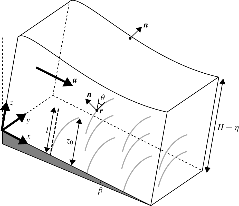
 $l$, which shall later be specified as elastic beams. A schematic of the set-up is given in figure 2.
Our main objective in the forthcoming sections is to derive a set of simplified equations that govern the interaction between fluid and vegetation. This model is an extension of models that have been previously developed by Dupont et al. (Reference Dupont, Gosselin, Py, de Langre, Hemon and Brunet2010) and Singh et al. (Reference Singh, Bandi, Mahadevan and Mandre2016), but with the difference that it allows both for free-surface displacement and for elastic deformation of the vegetation, which is therefore coupled with the flow.
2.1 Equations for the fluid
In a more complete model, the location of each physical plant surface must be calculated as part of the problem. However, provided that the cross-sectional length scale of the plant is much smaller than the separation of neighbouring plants, we can consider the far-field approximation of the momentum loss due to individual plants using a distribution of point forces in the Navier–Stokes equations. We thus consider an incompressible fluid in three dimensions with velocity  $\boldsymbol{u}=(u,v,w)$ at time
 $t$ satisfying
 $$\begin{eqnarray}\displaystyle & \displaystyle \unicode[STIX]{x1D735}\boldsymbol{\cdot }\boldsymbol{u}=0, & \displaystyle\end{eqnarray}$$
 $$\begin{eqnarray}\displaystyle & \displaystyle \unicode[STIX]{x1D70C}\left(\frac{\unicode[STIX]{x2202}\boldsymbol{u}}{\unicode[STIX]{x2202}t}+\boldsymbol{u}\boldsymbol{\cdot }\unicode[STIX]{x1D735}\boldsymbol{u}\right)=-\unicode[STIX]{x1D735}p+\unicode[STIX]{x1D70C}\boldsymbol{g}+\unicode[STIX]{x1D70C}\unicode[STIX]{x1D708}^{\ast }\unicode[STIX]{x1D6FB}^{2}\boldsymbol{u}+\boldsymbol{F}, & \displaystyle\end{eqnarray}$$
where  $\unicode[STIX]{x1D70C}$ is the density of water,
 $p$ is pressure,
 $\boldsymbol{g}=g(\sin \unicode[STIX]{x1D6FD},0,-\cos \unicode[STIX]{x1D6FD})$ is the acceleration due to gravity. It is important to account for eddies in the flow, which emerge from wakes of individual plants. To do so, we follow the approach by Singh et al. (Reference Singh, Bandi, Mahadevan and Mandre2016) and assign a constant eddy viscosity,
 $\unicode[STIX]{x1D708}^{\ast }$ in place of the kinematic viscosity of water. The additional sink term,
 $\boldsymbol{F}$, that appears in the momentum equation (2.2), incorporates the contribution of the
 $N$ plants; the precise form of
 $\boldsymbol{F}$ is discussed below.
Schematic diagram of flow through a portion of the canopy. The fluid domain above has flow velocity  $\boldsymbol{u}$, height
 $H+\unicode[STIX]{x1D702}$ and a free surface with outward normal
 $\bar{\boldsymbol{n}}$. The grey vegetative element with the centreline at
 $\boldsymbol{x}=(x,y,z)=\boldsymbol{r}$ denotes a plant that is rooted to the bottom substrate, which has an angle of inclination,
 $\unicode[STIX]{x1D6FD}$. The plant configuration is parametrised by arc length
 $s$ and local angle of deflection
 $\unicode[STIX]{x1D703}$. The vertical dashed line with length
 $l$ denotes the configuration when it is load free and
 $z_{0}$ is the height of the plant in the deformed configuration.

We model each of the  $N$ plants as a neutrally buoyant, inextensible linearly elastic beam with width (or diameter)
 $b$, which undergoes pure bending in the
 $(x,z)$-plane. We parametrise the centreline of the
 $k\text{th}$ beam by
 $\boldsymbol{x}=\boldsymbol{r}^{\,k}(s,\unicode[STIX]{x1D70F})$ where
 $s$ is arc length and
 $\unicode[STIX]{x1D70F}=t$ is time. We use
 $\unicode[STIX]{x1D70F}$ rather than
 $t$ to emphasise the implicit change of variables from
 $(\boldsymbol{x},t)$ to
 $(k,s,\unicode[STIX]{x1D70F})$; this is a Lagrangian description of the canopy. We shall return to this later in § 4.1 where we discuss the relationship between Eulerian and Lagrangian frames.
We assume that the collective sink term can be written as
 $$\begin{eqnarray}\boldsymbol{F}(\boldsymbol{x},t)\equiv \mathop{\sum }_{k=1}^{N}\boldsymbol{F}^{k}(\boldsymbol{x},t),\end{eqnarray}$$
with each individual term,  $\boldsymbol{F}^{k}$, accounting for the momentum loss due to the
 $k\text{th}$ plant. We note that, in § 2.3, we will homogenise the momentum loss of individual plants and consider a continuum approximation of
 $\boldsymbol{F}$. In considering the force balance on an object that is submerged in a fluid, we have to account for: (i) the loading on the object due to its surrounding fluid; (ii) the flow disturbance due to the motion of the object. For a neutrally buoyant cantilever beam, we have to account for drag
 $\boldsymbol{F}_{D}^{k}$, added mass
 $\boldsymbol{F}_{A}^{k}$ and virtual buoyancy
 $\boldsymbol{F}_{V}^{k}$ (Newman Reference Newman1977; Batchelor Reference Batchelor2000). Following previous analyses by Luhar & Nepf (Reference Luhar and Nepf2016) and Leclercq & de Langre (Reference Leclercq and de Langre2018), the component forces at a given
 $(\boldsymbol{x},t)$, determined via
 $\boldsymbol{F}^{k}=\boldsymbol{F}_{D}^{k}+\boldsymbol{F}_{A}^{k}+\boldsymbol{F}_{V}^{k}$ for a beam at position
 $\boldsymbol{x}=\boldsymbol{r}^{\,k}$ are as follows:
 $$\begin{eqnarray}\displaystyle & \displaystyle \boldsymbol{F}_{D}^{k}=-\frac{1}{2}\unicode[STIX]{x1D70C}bC_{D}\int _{0}^{l}\unicode[STIX]{x1D6FF}(\boldsymbol{x}-\boldsymbol{r}^{\,k})\left(\boldsymbol{u}-\frac{\unicode[STIX]{x2202}\boldsymbol{r}^{\,k}}{\unicode[STIX]{x2202}\unicode[STIX]{x1D70F}}\right)\boldsymbol{\cdot }\boldsymbol{n}^{k}\left|\left(\boldsymbol{u}-\frac{\unicode[STIX]{x2202}\boldsymbol{r}^{\,k}}{\unicode[STIX]{x2202}\unicode[STIX]{x1D70F}}\right)\boldsymbol{\cdot }\boldsymbol{n}^{k}\right|\boldsymbol{n}^{k}\,\text{d}s, & \displaystyle\end{eqnarray}$$
 $$\begin{eqnarray}\displaystyle & \displaystyle \boldsymbol{F}_{A}^{k}=-C_{M}m\int _{0}^{l}\unicode[STIX]{x1D6FF}(\boldsymbol{x}-\boldsymbol{r}^{\,k})\left[\left(\frac{\unicode[STIX]{x2202}\boldsymbol{u}}{\unicode[STIX]{x2202}t}-\frac{\unicode[STIX]{x2202}^{2}\boldsymbol{r}^{\,k}}{\unicode[STIX]{x2202}\unicode[STIX]{x1D70F}^{2}}\right)\boldsymbol{\cdot }\boldsymbol{n}^{k}\right]\boldsymbol{n}^{k}\,\text{d}s, & \displaystyle\end{eqnarray}$$
 $$\begin{eqnarray}\displaystyle & \displaystyle \boldsymbol{F}_{V}^{k}=-m\int _{0}^{l}\unicode[STIX]{x1D6FF}(\boldsymbol{x}-\boldsymbol{r}^{\,k})\frac{\unicode[STIX]{x2202}\boldsymbol{u}}{\unicode[STIX]{x2202}t}\,\text{d}s. & \displaystyle\end{eqnarray}$$
 $C_{D}$,
 $m$ and
 $C_{M}$, we consider a cross-section of unit length taken perpendicular to the axis of the beam, e.g. a circular cross-section for cylindrical beams. Then we write
 $C_{D}$ for its drag coefficient in cross-flow,
 $m$ for its mass and
 $C_{M}$ for its added mass coefficient; this last factor accounts for the amount of fluid the cross-section displaces when it translates perpendicularly to its axis. Note that for cylindrical beams,
 $C_{M}\approx 1$ (Brennen Reference Brennen1982). However, for cantilever blades with rectangular cross-sections, added mass effects are much more important than beam inertia and virtual buoyancy since
 $C_{M}\approx (\unicode[STIX]{x1D70C}\unicode[STIX]{x03C0}b^{2}/4)/m$ is expected to be large (Leclercq & de Langre Reference Leclercq and de Langre2018).
Within the integrals,  $\unicode[STIX]{x1D6FF}$ denotes the Dirac delta function and
 $\boldsymbol{n}^{k}$ is the upstream normal of the
 $k\text{th}$ beam’s centreline in the
 $(x,z)$-plane (cf. figure 2); if
 $\unicode[STIX]{x1D703}$ is the local angle of deflection at
 $s$, as measured from the upward vertical, then
 $\boldsymbol{n}^{k}=(-\text{cos}\,\unicode[STIX]{x1D703}^{k},0,\sin \unicode[STIX]{x1D703}^{k})$.
Our drag law (2.4a) can be interpreted as follows: for each element of arc length  $\text{d}s$, the drag element,
 $\text{d}\boldsymbol{F}_{D}^{k}$, corresponding to (2.4a) is the force a tilted cylinder of length
 $\text{d}s$ would experience (Sumer & Fredsøe Reference Sumer and Fredsøe2006). It has been argued both experimentally and numerically that this drag law is accurate until the beam approaches a configuration parallel to the flow (Ramberg Reference Ramberg1983; Vakil & Green Reference Vakil and Green2009; Zhao, Cheng & Zhou Reference Zhao, Cheng and Zhou2009). In the case of rigid and vertical beams, (2.4a) reduces to the formulation used in Singh et al. (Reference Singh, Bandi, Mahadevan and Mandre2016). We refer readers to Zhou et al. (Reference Zhou, Wang, Razali, Zhou and Cheng2010) for a more extensive review of drag on tilted cylinders, and also highlight that our drag law has also been used to compute blade drag in previous studies (e.g. by Luhar & Nepf (Reference Luhar and Nepf2016) and Leclercq & de Langre (Reference Leclercq and de Langre2018) for unsteady flows).
Finally, we note that we can model obstacles with spatial variations along the stem by incorporating non-uniform drag and added mass coefficients in  $\boldsymbol{F}$ (de Langre Reference de Langre2008).
2.2 Equations for the vegetation
Each individual plant is modelled as a linearly elastic beam with one end clamped perpendicularly to the substrate, and the other end is left free. Since the governing equations are identical for all plants  $k=1,\ldots ,N$, for the sake of clarity, we drop the superscript,
 $k$, for all of the variables in this subsection.
For each beam, let  $\boldsymbol{T}=(T_{1},T_{2},T_{3})$ be the internal stress and
 $\boldsymbol{M}$ be the moment on a cross-section given by position vector
 $\boldsymbol{r}$. By considering the momentum balance on this cross-section which has infinitesimal thickness,
 $\boldsymbol{T}$ satisfies (Landau et al. Reference Landau, Lifshitz, Sykes, Reid and Dill1960)
 $$\begin{eqnarray}\displaystyle \frac{\unicode[STIX]{x2202}\boldsymbol{T}}{\unicode[STIX]{x2202}s}+\boldsymbol{q}=m\frac{\unicode[STIX]{x2202}^{2}\boldsymbol{r}}{\unicode[STIX]{x2202}\unicode[STIX]{x1D70F}^{2}}, & & \displaystyle\end{eqnarray}$$
where  $\boldsymbol{q}$ is the external force per unit length on the beam. We also consider the angular momentum balance on this cross-section. Noting that
 $\unicode[STIX]{x2202}\boldsymbol{r}/\unicode[STIX]{x2202}s=(\sin \unicode[STIX]{x1D703},0,\cos \unicode[STIX]{x1D703})$ is the local tangent vector of the plant, if we assume that the standard constitutive relation between
 $\boldsymbol{M}$ and
 $\boldsymbol{r}$ holds under dynamic conditions, namely (Landau et al. Reference Landau, Lifshitz, Sykes, Reid and Dill1960)
 $$\begin{eqnarray}\boldsymbol{M}=EI\frac{\unicode[STIX]{x2202}\boldsymbol{r}}{\unicode[STIX]{x2202}s}\times \frac{\unicode[STIX]{x2202}^{2}\boldsymbol{r}}{\unicode[STIX]{x2202}s^{2}},\end{eqnarray}$$
then  $\unicode[STIX]{x1D703}$ satisfies (McMillen & Goriely Reference McMillen and Goriely2003)
 $$\begin{eqnarray}\displaystyle \frac{\unicode[STIX]{x2202}}{\unicode[STIX]{x2202}s}\left(EI\frac{\unicode[STIX]{x2202}\unicode[STIX]{x1D703}}{\unicode[STIX]{x2202}s}\right)+T_{1}\cos \unicode[STIX]{x1D703}-T_{3}\sin \unicode[STIX]{x1D703}=\unicode[STIX]{x1D70C}I\frac{\unicode[STIX]{x2202}^{2}\unicode[STIX]{x1D703}}{\unicode[STIX]{x2202}\unicode[STIX]{x1D70F}^{2}}. & & \displaystyle\end{eqnarray}$$
In this equation,  $E$ is the Young’s modulus and
 $I$ is the moment of inertia of the cross-section about the
 $y$-axis. The bending term is expressed in a form such that the beam equations, equations (2.5) and (2.7), can model beams with a non-uniform cross-section
 $b=b(s)$. However, in this work, we consider
 $b$ constant.
Finally, we must determine the total external load on the plant,  $\boldsymbol{q}=\boldsymbol{q}(s,\unicode[STIX]{x1D70F})$, in (2.5). As discussed in § 2.1, the momentum loss in the fluid balances the load on the plant. Thus, with reference to the component forces of
 $\boldsymbol{F}^{k}$ in (2.4), the total load is given by
 $\boldsymbol{q}=\boldsymbol{q}_{D}+\boldsymbol{q}_{A}+\boldsymbol{q}_{V}$. These individual loads
 $\boldsymbol{q}_{D}$,
 $\boldsymbol{q}_{A}$ and
 $\boldsymbol{q}_{V}$, are considered to be functions of
 $s$ and
 $\unicode[STIX]{x1D70F}$, with
 $$\begin{eqnarray}\displaystyle & \displaystyle \boldsymbol{q}_{D}=\frac{1}{2}\unicode[STIX]{x1D70C}bC_{D}\int _{\unicode[STIX]{x1D6FA}}\unicode[STIX]{x1D6FF}(\boldsymbol{x}-\boldsymbol{r})\left(\boldsymbol{u}-\frac{\unicode[STIX]{x2202}\boldsymbol{r}}{\unicode[STIX]{x2202}\unicode[STIX]{x1D70F}}\right)\boldsymbol{\cdot }\boldsymbol{n}\left|\left(\boldsymbol{u}-\frac{\unicode[STIX]{x2202}\boldsymbol{r}}{\unicode[STIX]{x2202}\unicode[STIX]{x1D70F}}\right)\boldsymbol{\cdot }\boldsymbol{n}\right|\boldsymbol{n}\,\text{d}\boldsymbol{x}, & \displaystyle\end{eqnarray}$$
 $$\begin{eqnarray}\displaystyle & \displaystyle \boldsymbol{q}_{A}=C_{M}m\int _{\unicode[STIX]{x1D6FA}}\unicode[STIX]{x1D6FF}(\boldsymbol{x}-\boldsymbol{r})\left[\left(\frac{\unicode[STIX]{x2202}\boldsymbol{u}}{\unicode[STIX]{x2202}t}-\frac{\unicode[STIX]{x2202}^{2}\boldsymbol{r}}{\unicode[STIX]{x2202}\unicode[STIX]{x1D70F}^{2}}\right)\boldsymbol{\cdot }\boldsymbol{n}\right]\boldsymbol{n}\,\text{d}\boldsymbol{x}, & \displaystyle\end{eqnarray}$$
 $$\begin{eqnarray}\displaystyle & \displaystyle \boldsymbol{q}_{V}=m\int _{\unicode[STIX]{x1D6FA}}\unicode[STIX]{x1D6FF}(\boldsymbol{x}-\boldsymbol{r})\frac{\unicode[STIX]{x2202}\boldsymbol{u}}{\unicode[STIX]{x2202}t}\,\text{d}\boldsymbol{x}, & \displaystyle\end{eqnarray}$$
 $\unicode[STIX]{x1D6FA}$ is the fluid domain.
2.3 Homogenisation of the canopy
Even with the simplifications we have made so far, it is impractical to monitor the positions and effects of individual plants in the flow. Instead, we use a simpler averaged model in which the canopy is an effective medium which contributes a bulk volumetric sink term (see e.g. Nepf (Reference Nepf2012) and the references therein for previous models in this direction). Here, we briefly present the derivation of such a model by volume averaging.
Consider a fixed  $\boldsymbol{x}=(x,y,z)$. We define
 $\overline{\boldsymbol{F}}_{R}$ as the local average of the collective sink over a disk of radius
 $R$, namely
 $$\begin{eqnarray}\overline{\boldsymbol{F}}_{R}(\boldsymbol{x},t)=\frac{1}{\unicode[STIX]{x03C0}R^{2}}\iint _{C_{R}(x,y;z)}\boldsymbol{F}(\boldsymbol{x}^{\prime },t)\,\text{d}x^{\prime }\,\text{d}y^{\prime },\end{eqnarray}$$
where  $C_{R}(x,y;z)$ is the two-dimensional disk of radius
 $R$ centred at the point
 $\boldsymbol{x}$ i.e.
 $$\begin{eqnarray}C_{R}(x,y;z)=\{(x^{\prime },y^{\prime },z):(x-x^{\prime })^{2}+(y-y^{\prime })^{2}\leqslant R\}\end{eqnarray}$$
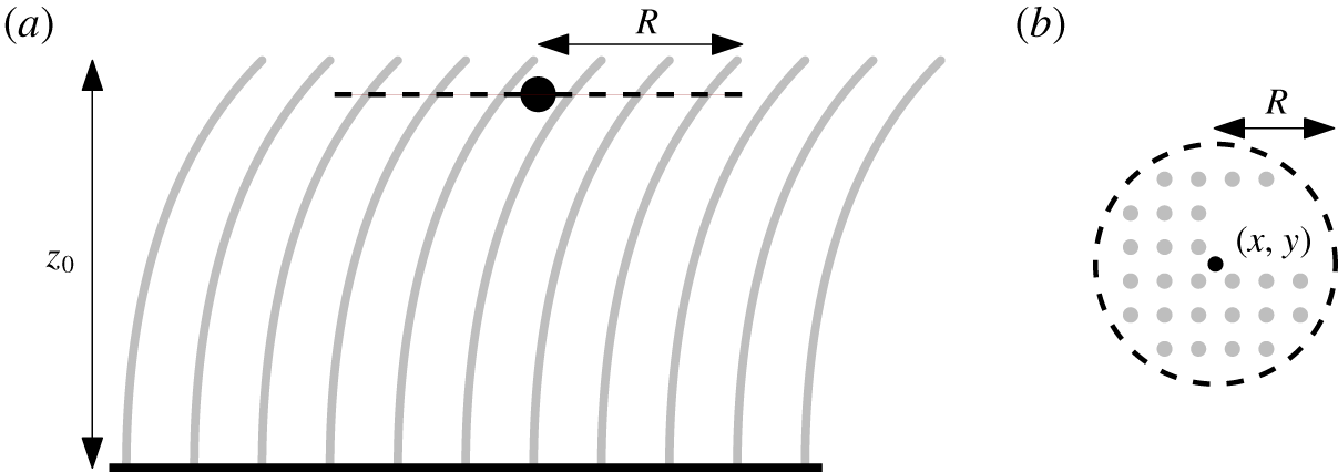
(see figure 3). By the definition of  $\boldsymbol{F}$ in (2.3),
 $$\begin{eqnarray}\overline{\boldsymbol{F}}_{R}(\boldsymbol{x},t)=\frac{1}{\unicode[STIX]{x03C0}R^{2}}\iint _{C_{R}(x,y;z)}\left[\mathop{\sum }_{k=1}^{N}\int _{0}^{l}\boldsymbol{Q}^{k}\unicode[STIX]{x1D6FF}(\boldsymbol{x}^{\prime }-\boldsymbol{r}^{\,k})\,\text{d}s\right]\,\text{d}x^{\prime }\,\text{d}y^{\prime },\end{eqnarray}$$
where
 $$\begin{eqnarray}\displaystyle \boldsymbol{Q}^{k} & = & \displaystyle -\frac{1}{2}\unicode[STIX]{x1D70C}bC_{D}\left(\boldsymbol{u}-\frac{\unicode[STIX]{x2202}\boldsymbol{r}^{\,k}}{\unicode[STIX]{x2202}\unicode[STIX]{x1D70F}}\right)\boldsymbol{\cdot }\boldsymbol{n}^{k}\left|\left(\boldsymbol{u}-\frac{\unicode[STIX]{x2202}\boldsymbol{r}^{\,k}}{\unicode[STIX]{x2202}\unicode[STIX]{x1D70F}}\right)\boldsymbol{\cdot }\boldsymbol{n}^{k}\right|\boldsymbol{n}^{k}\nonumber\\ \displaystyle & & \displaystyle -\,C_{M}m\left[\left(\frac{\unicode[STIX]{x2202}\boldsymbol{u}}{\unicode[STIX]{x2202}t}-\frac{\unicode[STIX]{x2202}^{2}\boldsymbol{r}^{\,k}}{\unicode[STIX]{x2202}\unicode[STIX]{x1D70F}^{2}}\right)\boldsymbol{\cdot }\boldsymbol{n}^{k}\right]\boldsymbol{n}^{k}-m\frac{\unicode[STIX]{x2202}\boldsymbol{u}}{\unicode[STIX]{x2202}t}.\end{eqnarray}$$
Now, by definition,
 $$\begin{eqnarray}\unicode[STIX]{x1D6FF}(\boldsymbol{x}^{\prime }-\boldsymbol{r}^{\,k})=\unicode[STIX]{x1D6FF}(x^{\prime }-r_{1}^{k})\unicode[STIX]{x1D6FF}(y^{\prime }-r_{2}^{k})\unicode[STIX]{x1D6FF}(z-r_{3}^{k}).\end{eqnarray}$$
In order to sample plants that pass through  $C_{R}$, we rewrite the
 $s$-integral in (2.11) with respect to
 $z$. Assuming that the beam configurations do not overturn,
 $$\begin{eqnarray}\frac{\text{d}}{\text{d}s}=\frac{\text{d}z}{\text{d}s}\frac{\text{d}}{\text{d}z}=\cos \unicode[STIX]{x1D703}^{k}\frac{\text{d}}{\text{d}z}.\end{eqnarray}$$
Therefore,
 $$\begin{eqnarray}\displaystyle \overline{\boldsymbol{F}}_{R}(\boldsymbol{x},t)=\frac{1}{\unicode[STIX]{x03C0}R^{2}}\mathop{\sum }_{k=1}^{N}\boldsymbol{Q}^{k}(\boldsymbol{r}^{\,k},t)\unicode[STIX]{x1D7D9}_{R}^{k}(\boldsymbol{x},t)\sec \unicode[STIX]{x1D703}^{k}(z,t), & & \displaystyle\end{eqnarray}$$
where  $\unicode[STIX]{x1D7D9}_{R}^{k}$ is an indicator function with
 $\unicode[STIX]{x1D7D9}_{R}^{k}(\boldsymbol{x},t)=1$ if the
 $k\text{th}$ plant passes through
 $C_{R}$ (and zero otherwise).
Schematic diagram of  $C_{R}(x,y;z)$: a circle of radius
 $R$ (dashed), centred at
 $\boldsymbol{x}=(x,y,z)$, encircling a collection of plants (in grey) in the canopy. (a) Side view of the circle. (b) Top view of the circle.

We now consider the limit in which  $R\rightarrow 0$ (with the neighbouring plant separation also tending to zero so that there are still many plants crossing
 $C_{R}$). Since we have assumed that the plants are identical in the canopy, we approximate
 $\boldsymbol{u}$ to be uniform in
 $C_{R}$ and similarly for the configuration and motion of the plants. With reference to the local averaging argument presented by Chapman (Reference Chapman1995), we deduce the continuum approximation of
 $\boldsymbol{F}$ as
 $$\begin{eqnarray}\displaystyle \overline{\boldsymbol{F}}=\lim _{R\rightarrow 0}\overline{\boldsymbol{F}}_{R}=-\bar{N}\sec \unicode[STIX]{x1D703}\text{H}(z_{0}-z)\boldsymbol{Q}(\boldsymbol{x},t), & & \displaystyle\end{eqnarray}$$
where  $\bar{N}(x,y)$ is the number of plants planted per unit area (along the bottom substrate) and
 $\text{H}$ is the Heaviside step function. The dependence of
 $\overline{\boldsymbol{F}}$ on
 $\sec \unicode[STIX]{x1D703}$ physically corresponds to the perpendicular distance between neighbouring plants being reduced when they tilt, so that the effective density of the canopy increases. For the remainder of this work, we will consider uniform canopies where
 $\overline{N}$ is constant and replace
 $\boldsymbol{F}$ with
 $\overline{\boldsymbol{F}}$ in the Navier–Stokes equations (2.1)–(2.2).
2.4 Simplification and non-dimensionalisation
Before continuing, we highlight two further simplifying assumptions that we will make. Firstly, along the bottom substrate, we impose a shear-free condition for the fluid based on the negligible size of the boundary layer there (Dunn et al. Reference Dunn, Lopez and García1996; Ghisalberti & Nepf Reference Ghisalberti and Nepf2002). We shall revisit this simplification in the final discussion in § 9. Secondly, we focus on the typical scenario where the speed of sound in a beam,  $\sqrt{E/\unicode[STIX]{x1D70C}}$, is much greater than the velocity scale of the fluid,
 $U$; in this case, the inertial term in the beam equation (2.7) can be neglected.
We non-dimensionalise the variables in our problem with the following scales:
 $$\begin{eqnarray}[x]=[z]=[s]=H,\quad [\boldsymbol{u}]=U,\quad [t]=\frac{H}{U},\quad [p]=\unicode[STIX]{x1D70C}U^{2},\quad [\boldsymbol{T}]=\unicode[STIX]{x1D70C}bC_{D}HU^{2}.\end{eqnarray}$$
Foreseeing the calculations ahead, we take  $U$ to be the streamwise velocity at the free surface for steady unidirectional flows: we will specify such flows in § 3.
With all the variables being henceforth dimensionless, we have following system of equations:
 $$\begin{eqnarray}\displaystyle & \displaystyle \unicode[STIX]{x1D735}\boldsymbol{\cdot }\boldsymbol{u}=0, & \displaystyle\end{eqnarray}$$
 $$\begin{eqnarray}\displaystyle & \displaystyle \frac{\unicode[STIX]{x2202}\boldsymbol{u}}{\unicode[STIX]{x2202}t}+\boldsymbol{u}\boldsymbol{\cdot }\unicode[STIX]{x1D735}\boldsymbol{u}=-\unicode[STIX]{x1D735}p+\frac{1}{Fr^{2}}\boldsymbol{g}+{\displaystyle \frac{1}{Re^{\ast }}}\unicode[STIX]{x1D6FB}^{2}\boldsymbol{u}-\unicode[STIX]{x1D706}\sec \unicode[STIX]{x1D703}\text{H}(z_{0}-z)\boldsymbol{q}, & \displaystyle\end{eqnarray}$$
 $$\begin{eqnarray}\displaystyle & \displaystyle \frac{\unicode[STIX]{x2202}\boldsymbol{T}}{\unicode[STIX]{x2202}s}+\boldsymbol{q}=M_{2}\frac{\unicode[STIX]{x2202}^{2}\boldsymbol{r}}{\unicode[STIX]{x2202}\unicode[STIX]{x1D70F}^{2}}, & \displaystyle\end{eqnarray}$$
 $$\begin{eqnarray}\displaystyle & \displaystyle \frac{\unicode[STIX]{x2202}^{2}\unicode[STIX]{x1D703}}{\unicode[STIX]{x2202}s^{2}}=C_{Y}(-T_{1}\cos \unicode[STIX]{x1D703}+T_{3}\sin \unicode[STIX]{x1D703}), & \displaystyle\end{eqnarray}$$
where
 $$\begin{eqnarray}\boldsymbol{q}=\frac{1}{2}\left(\boldsymbol{u}-\frac{\unicode[STIX]{x2202}\boldsymbol{r}}{\unicode[STIX]{x2202}\unicode[STIX]{x1D70F}}\right)\boldsymbol{\cdot }\boldsymbol{n}\left|\left(\boldsymbol{u}-\frac{\unicode[STIX]{x2202}\boldsymbol{r}}{\unicode[STIX]{x2202}\unicode[STIX]{x1D70F}}\right)\boldsymbol{\cdot }\boldsymbol{n}\right|\boldsymbol{n}+M_{1}\left[\left(\frac{\unicode[STIX]{x2202}\boldsymbol{u}}{\unicode[STIX]{x2202}t}-\frac{\unicode[STIX]{x2202}^{2}\boldsymbol{r}}{\unicode[STIX]{x2202}\unicode[STIX]{x1D70F}^{2}}\right)\boldsymbol{\cdot }\boldsymbol{n}\right]\boldsymbol{n}+M_{2}\frac{\unicode[STIX]{x2202}\boldsymbol{u}}{\unicode[STIX]{x2202}t}.\end{eqnarray}$$
With  $\unicode[STIX]{x1D748}$ as the fluid stress tensor, the corresponding boundary conditions are


The dimensionless parameters  $Re^{\ast }$,
 $Fr$,
 $h$,
 $\unicode[STIX]{x1D706}$,
 $M_{1}$,
 $M_{2}$ and
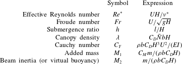
 $C_{Y}$ are defined in table 2. In particular,
 $\unicode[STIX]{x1D706}$ is the product of the dimensionless planting density,
 $\bar{N}H^{2}$, the aspect ratio,
 $b/H$, and the geometry factor,
 $C_{D}$.
For each beam, the parameters  $M_{1}$ and
 $M_{2}$ characterise the respective effects of added mass and beam inertia (or virtual buoyancy) relative to drag. Finally,
 $C_{Y}$ characterises the balance between static deflection and loading due to drag. We have chosen the convention where we incorporate the geometry of the plant by scaling
 $C_{Y}$ with
 $C_{D}$ and
 $I$ instead of introducing a slenderness parameter (de Langre Reference de Langre2008).
A summary of the dimensionless parameters in the governing equations of flow through a homogenised canopy (2.18).

We have seen in (2.18) that it is natural to write the Navier–Stokes equations in Eulerian coordinates but it is more natural to write the beam equations in body-fitted coordinates (i.e. arc length  $s$). These systems are related via
 $\unicode[STIX]{x2202}\boldsymbol{r}/\unicode[STIX]{x2202}s=(\sin \unicode[STIX]{x1D703},0,\cos \unicode[STIX]{x1D703})$. We examine the translation between the two coordinate systems more fully in § 4.1.
3 Steady unidirectional flow
In this section, we seek solutions of the governing system (2.18) where the flow is steady and unidirectional along the  $x$-axis (the streamwise direction), with
 $$\begin{eqnarray}\boldsymbol{u}=u(z)\hat{\boldsymbol{e}}_{x}.\end{eqnarray}$$
The study of unidirectional flows provides not only significant mathematical reduction, but is also justified by many related experiments. For example, such flows emerge from current-dominated flows in experimental flumes with vegetation. As a result, field studies, controlled experiments and, more recently, numerical simulations typically consider such flows (cf. Nepf (Reference Nepf2012) and references therein).
If the canopy is finite, we note that there exists a transition region for the incoming flow starting from the leading edge of the canopy (Chen, Jiang & Nepf Reference Chen, Jiang and Nepf2013). The mixed conclusions on how to systematically predict this development length have typically resulted in calibrations and verifications in individual experiments (see e.g. Dunn et al. (Reference Dunn, Lopez and García1996), Ghisalberti & Nepf (Reference Ghisalberti and Nepf2004)). The flow then settles beyond this region. Hence, when we consider steady unidirectional flows of the form stated above in (3.1), we are only considering the fully developed regions downstream.
3.1 Theoretical formulation
Since the flow is both steady and unidirectional, we can deduce from the momentum equation of the fluid (2.2) that the free surface is flat at  $z=1$ and the flow is driven by a constant pressure gradient. It is particularly convenient to re-write the pressure,
 $p$, in terms of the dynamic fluid pressure,
 $$\begin{eqnarray}\bar{p}=p-\frac{1}{Fr^{2}}(x\sin \unicode[STIX]{x1D6FD}-z\cos \unicode[STIX]{x1D6FD}),\end{eqnarray}$$
which we use for the remainder of this work. The governing equations (2.18) reduce to the following system of differential equations:
 $$\begin{eqnarray}\displaystyle & \displaystyle \frac{\text{d}^{2}u}{\text{d}z^{2}}=-Re^{\ast }P+\text{H}(z_{0}-z)\frac{Re^{\ast }\unicode[STIX]{x1D706}}{2}u\cos \unicode[STIX]{x1D703}|u\cos \unicode[STIX]{x1D703}|, & \displaystyle\end{eqnarray}$$
 $$\begin{eqnarray}\displaystyle & \displaystyle \frac{\text{d}T_{1}}{\text{d}s}=-{\displaystyle \frac{1}{2}}u\cos ^{2}\unicode[STIX]{x1D703}|u\cos \unicode[STIX]{x1D703}|, & \displaystyle\end{eqnarray}$$
 $$\begin{eqnarray}\displaystyle & \displaystyle \frac{\text{d}T_{3}}{\text{d}s}={\displaystyle \frac{1}{2}}u\sin \unicode[STIX]{x1D703}\cos \unicode[STIX]{x1D703}|u\cos \unicode[STIX]{x1D703}|, & \displaystyle\end{eqnarray}$$
 $$\begin{eqnarray}\displaystyle & \displaystyle \frac{\text{d}^{2}\unicode[STIX]{x1D703}}{\text{d}s^{2}}=C_{Y}(-T_{1}\cos \unicode[STIX]{x1D703}+T_{3}\sin \unicode[STIX]{x1D703}), & \displaystyle\end{eqnarray}$$
 $P=\sin \unicode[STIX]{x1D6FD}/Fr^{2}>0$ is imposed such that
 $u(1)=1$ (i.e. the velocity scale
 $U$ in
 $Fr$ is chosen to make
 $u(1)=1$). To solve for the steady configuration, we rewrite equations (3.3) as a system of ordinary differential equations in
 $z$ and solve the equations numerically (with the corresponding boundary conditions in (2.18)) in MATLAB using the boundary value problem solver bvp4c. Once we obtain the solution, the centreline of the homogenised plant configuration,
 $\boldsymbol{r}$, can be determined in Cartesian coordinates from the relation
 $$\begin{eqnarray}\frac{\text{d}x}{\text{d}z}=\tan \unicode[STIX]{x1D703}.\end{eqnarray}$$
As an aside, we note that our model predicts a parabolic flow profile above the canopy rather than logarithmic as in classic boundary-layer flows (Nikora Reference Nikora2010). Since the canopy enhances flow mixing above the canopy, it has been experimentally shown that the logarithmic scaling is only recovered when  $z\gtrapprox 2h$ (see Sharma & García-Mayoral (Reference Sharma and García-Mayoral2018) and references therein). Provided that
 $h=O(1)$, which is typical for aquatic vegetation (Nepf Reference Nepf2012), we can assume that we are not in the logarithmic regime. For flows with
 $h\ll 1$, the transition zone where
 $h\leqslant z\lessapprox 2h$ is known as the roughness sublayer (Finnigan Reference Finnigan2000).
3.2 Unidirectional flows through rigid canopies ( $C_{Y}=0$)

We first examine the case of flow through a rigid canopy, considering the limits of sparse and dense canopies.
3.2.1 Asymptotic approximation of $u$ for sparse canopies ($\unicode[STIX]{x1D706}\ll 1$)


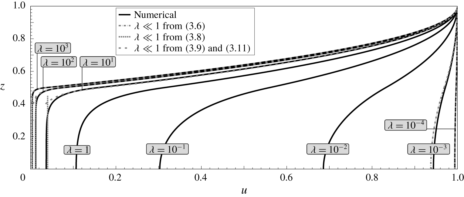
The velocity profiles at different values of the canopy density parameter  $\unicode[STIX]{x1D706}$ are shown in figure 4. In the limit the canopy density tends to zero, the velocity profile approaches that corresponding to uniform unobstructed flow. Noting that a more convenient perturbation parameter is
 $Re^{\ast }\unicode[STIX]{x1D706}$, we let
 $u=1+Re^{\ast }\unicode[STIX]{x1D706}\tilde{u}$ and
 $P=\unicode[STIX]{x1D706}\tilde{P}$. Then, by (3.3a), we have
 $$\begin{eqnarray}\frac{\text{d}^{2}\tilde{u} }{\text{d}z^{2}}\sim \left\{\begin{array}{@{}ll@{}}-\tilde{P}+\displaystyle \frac{1}{2},\quad & \text{if}~z\leqslant h,\\[5.69054pt] -\tilde{P},\quad & \text{if}~z>h.\end{array}\right.\end{eqnarray}$$
By solving for  $\tilde{u}$ (and
 $\tilde{P}$), we deduce that
 $$\begin{eqnarray}u=1+Re^{\ast }\unicode[STIX]{x1D706}\tilde{u} \sim \left\{\begin{array}{@{}ll@{}}1-{\displaystyle \frac{Re^{\ast }\unicode[STIX]{x1D706}}{4}}(1-h)(h-z^{2}),\quad & \text{if}~z\leqslant h,\\ 1-{\displaystyle \frac{Re^{\ast }\unicode[STIX]{x1D706}}{4}}h\left(z-1\right)^{2},\quad & \text{if}~z>h,\end{array}\right.\end{eqnarray}$$
confirming the behaviour illustrated in figure 4. In particular, as the canopy density increases, the flow velocity reduces everywhere due to increased drag; however, as expected, the reduction is greatest within the canopy itself ( $z\leqslant h$).
The effect of increasing canopy density to steady unidirectional flows through a rigid canopy when  $Re^{\ast }=10^{3}$ and
 $h=0.5$. Flow profiles are shown in black solid lines with grey lines indicating asymptotic approximations as described in § 3.2.

3.2.2 Asymptotic approximation of $u$ for dense canopies $(\unicode[STIX]{x1D706}\gg 1)$


We also observe from figure 4 that, in the dense-canopy limit, the flow is apparently divided into two outer regions ( $z<h$ and
 $z>h$), as well as a transition region near
 $z=h$. In the limit
 $\unicode[STIX]{x1D706}\rightarrow \infty$, we observe that the flow becomes approximately uniform in the canopy, where
 $0\leqslant z\leqslant h$ and
 $h-z=O(1)$. From (3.3a), we have that in this region,
 $$\begin{eqnarray}\frac{\text{d}^{2}u}{\text{d}z^{2}}=-Re^{\ast }P+\frac{Re^{\ast }\unicode[STIX]{x1D706}}{2}u|u|,\end{eqnarray}$$
and thus to leading order, the pressure gradient balances the drag, and the velocity below the canopy satisfies
 $$\begin{eqnarray}u_{below}(z)\sim \left(\frac{2P}{\unicode[STIX]{x1D706}}\right)^{1/2}\quad \text{for }0\leqslant z\leqslant h\text{ and }h-z=O(1).\end{eqnarray}$$
This matches the result of Poggi et al. (Reference Poggi, Porporato, Ridolfi, Albertson and Katul2004, §5) and Singh et al. (Reference Singh, Bandi, Mahadevan and Mandre2016, §3). This approximation is plotted with dotted lines in figure 4.
Before deriving the solution in the boundary layer at the top of the canopy, we note that the solution for  $z\geqslant h$ can be found exactly: integrating (3.3a) and applying the surface boundary conditions,
 $u(1)=1$ and
 $u^{\prime }(1)=0$, we find that for the solution above the canopy,
 $$\begin{eqnarray}u_{above}(z)=Re^{\ast }P\left(z-\frac{z^{2}}{2}-\frac{1}{2}\right)+1\quad \text{for }z\geqslant h.\end{eqnarray}$$
Note that the constant quantity,  $P$, itself must be expanded in
 $\unicode[STIX]{x1D706}$ and will be determined through boundary conditions. In the inner region, we substitute
 $z=h-\unicode[STIX]{x1D706}^{-1/3}\unicode[STIX]{x1D709}$ and
 $u=\unicode[STIX]{x1D706}^{-1/3}\tilde{u}$ into (3.3a) with
 $\unicode[STIX]{x1D709}\geqslant 0$. The inner solution satisfies
 $$\begin{eqnarray}\left(\frac{\text{d}\tilde{u} }{\text{d}\unicode[STIX]{x1D709}}\right)^{2}\sim \frac{Re^{\ast }}{3}\tilde{u} ^{3}+C,\end{eqnarray}$$
where the integration constant  $C=0$ in order to match (3.8) to this order of approximation. As a result, taking the relevant branch of (3.10) and requiring that the solution is continuous with (3.9), we have that for the solution within the boundary layer,
 $$\begin{eqnarray}u_{layer}(z)\sim \left[\left(\frac{Re^{\ast }\unicode[STIX]{x1D706}}{12}\right)^{1/2}(h-z)+\left\{1-\frac{Re^{\ast }P}{2}\left(1-h\right)^{2}\right\}^{-1/2}\right]^{-2},\end{eqnarray}$$
which is valid for  $z\leqslant h$ and
 $h-z=O(\unicode[STIX]{x1D706}^{-1/3})$. Finally, in order to determine the leading-order behaviour of the constant pressure gradient,
 $P$, we require that the gradient of (3.9) matches that given by the boundary layer of (3.10) at
 $z=h$. This yields
 $$\begin{eqnarray}P\sim \frac{2}{Re^{\ast }(1-h)^{2}}\left(1-\left[\frac{12}{Re^{\ast }\unicode[STIX]{x1D706}(1-h)^{2}}\right]^{1/3}\right).\end{eqnarray}$$
Note that in the above expression, we have retained the first two orders in  $P$ so as to ensure higher accuracy in the above-canopy solution for a wider range of
 $\unicode[STIX]{x1D706}$ values. In figure 4, we observe good agreement between the exact numerical flow profiles and the matched-asymptotic approximations given in (3.9) and (3.11).
3.3 Unidirectional flows through flexible canopies ($C_{Y}\neq 0$)

Having gained some intuition on flows through rigid canopies, we now explore the differences in flows through flexible canopies – the main motivation of this work. Before we continue, we first define how we will vary the flexibility. We recall from § 2 that the Cauchy number,  $C_{Y}$, characterises the amount of deflection due to drag. Hence, it varies with the velocity scale (cf. table 2). In order to vary flexibility independently of velocity, we vary the ratio
 $$\begin{eqnarray}\frac{C_{Y}}{Re^{\ast 2}}=\frac{\unicode[STIX]{x1D70C}C_{D}bH\unicode[STIX]{x1D708}^{\ast 2}}{EI}\end{eqnarray}$$
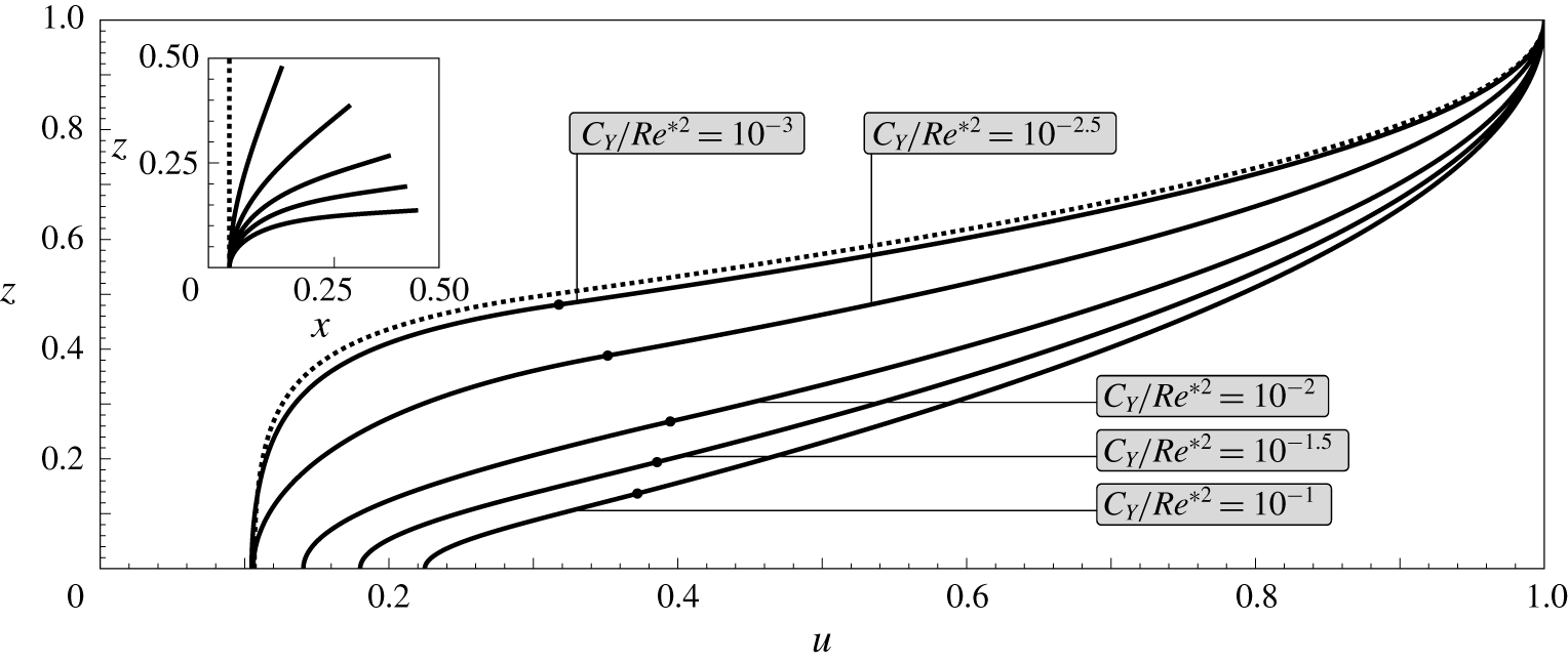
in our analysis for the remainder of this work. Flow profiles for varying  $C_{Y}/Re^{\ast 2}$ and fixed canopy density are shown in figure 5.
The effect of increasing the flexibility of vegetation to steady unidirectional flows when  $Re^{\ast }=10^{3}$,
 $\unicode[STIX]{x1D706}=1$ and
 $h=0.5$. Flow profiles are shown in solid lines for different values of
 $C_{Y}/Re^{\ast 2}$, with the corresponding homogenised beam configuration (to scale) in the inset. Dots in the main figure indicate the respective height of the canopy and dotted lines indicate the configuration in the rigid-canopy limit
 $C_{Y}/Re^{\ast 2}=0$.

As for flows through rigid canopies, every flow profile in figure 5 increases monotonically in  $z$ and inflects at the top of the canopy. As we increase the flexibility of the vegetation (by increasing
 $C_{Y}/Re^{\ast 2}$), less of the domain is obstructed, and we get faster flows at any given
 $z$. For applications such as flood control, if we use the (dimensional) maximum velocity as a simple measure for damage, the results suggest that upright obstacles attenuate a steady flow most effectively. We will revisit this conclusion in the next section when we consider the unsteady problem.
As an aside, we note that for regimes where the canopy is dense ( $\unicode[STIX]{x1D706}\gg 1$), we expect the approximations in § 3.2.2 to hold for plants that are sufficiently stiff. In this limit, since
 $u=O(\unicode[STIX]{x1D706}^{-1/3})$, the load, and hence the deflection, of each plant is negligible.
3.3.1 Height-averaged in-canopy velocity
One quantity of practical interest is the in-canopy velocity, considered by many studies on canopy physics (see Nepf (Reference Nepf2012) and references therein). Note that our choice of non-dimensionalisation makes it easy to compare between the in-canopy flow and the unobstructed flow. Since velocities are scaled with the free-surface velocity, the height-averaged dimensionless in-canopy velocity,  $\overline{u}_{c}$ say, corresponds to the ratio between the canopy and free-surface velocities.
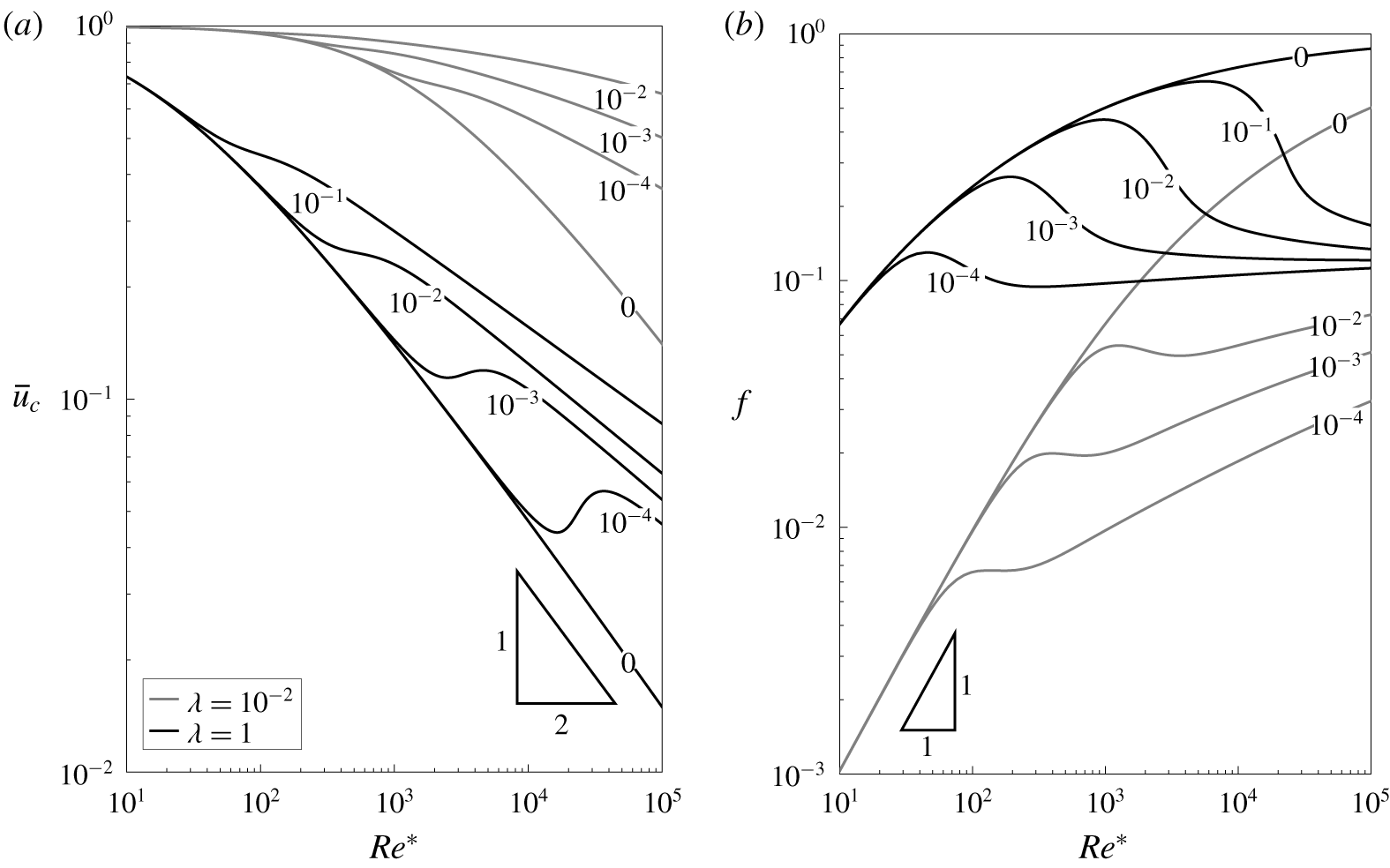
We observe from figure 6(a) that when canopy effects are negligible, which corresponds to the canopy being sparse or the Reynolds number low,  $\overline{u}_{c}\rightarrow 1$. As canopy effects become more prominent, we can infer from the analysis in § 3.2 that, for rigid canopies,
 $\overline{u}_{c}=O((Re^{\ast }\unicode[STIX]{x1D706})^{-1/2})$. For flexible canopies, however,
 $\overline{u}_{c}$ is not monotonic, as the plants transition from being upright to fully bent over with increasing Reynolds number. The slower decay of
 $\overline{u}_{c}$ for fully bent-over plants can be explained by drag being negligible along most of the length of the plant, apart from a boundary layer near the root, where the plant is forced upright by the clamped condition.
Height-averaged in-canopy velocity  $\overline{u}_{c}$ in (a), and relative canopy drag
 $f$ (3.14) in (b), versus
 $Re^{\ast }$ for
 $h=0.5$, with canopy density
 $\unicode[STIX]{x1D706}=1$ (shown black) and
 $\unicode[STIX]{x1D706}=10^{-2}$ (shown grey). Labels on the solid lines indicate plant flexibility,
 $C_{Y}/Re^{\ast 2}$.

3.3.2 Canopy drag, pressure gradient and flux
Another quantity of practical is the canopy drag. Typically, drag is defined in terms of velocity. However, it is difficult to compare the drag between two flows if the flux is not fixed. Consequently, to specify a non-dimensional measure of the drag on the flow which is easier to interpret, we define
 $$\begin{eqnarray}f=a\frac{Re^{\ast }P}{Q},\end{eqnarray}$$
where  $Q$ is the dimensionless flux and the scale factor
 $a$ is chosen such that
 $f=1$ when the canopy is infinitely dense, corresponding to (the lower half of) a Poiseuille flow in
 $z\in [h,1]$. Thus, for less dense canopies,
 $f$ represents the relative pressure gradient required to generate the same flux as this Poiseuille flow. As a result, we can directly compare drag between any two flows by comparing
 $f$, and this permits a number of interesting observations.
For rigid canopies, since the classic expression for drag scales with velocity squared,  $f$ monotonically increases with the Reynolds number. For instance, we can deduce from the analysis in § 3.2 that
 $f=O(Re^{\ast }\unicode[STIX]{x1D706})$ when
 $Re^{\ast }\unicode[STIX]{x1D706}\ll 1$, whilst, for high Reynolds numbers, rigid-canopy flows become akin to the classic Poiseuille flow i.e.
 $f\rightarrow 1$. For flexible canopies however, as with the in-canopy velocity, we observe in figure 6(b) that there is non-monotonic behaviour as the plants transition from being upright to fully bent over. In contrast to rigid-canopy flows, there is an interesting competition between the effects of increasing the Reynolds number and canopy reconfiguration.
4 Stability analysis of the steady configuration
Our main task in this section is to extend the stability analysis of Singh et al. (Reference Singh, Bandi, Mahadevan and Mandre2016) for rigid canopies to flexible canopies with a free surface. By modelling the canopy as an array of elastic beams, we are interested in the temporal evolution of both the perturbed flow and the canopy configuration.
By considering the steady configurations of § 3 as base states, we first derive the system of equations the perturbations satisfy at leading order. We then impose a spectral decomposition on the perturbations and solve the corresponding quadratic eigenvalue problem numerically. In this work, we consider two-dimensional disturbances in the  $(x,z)$-plane, which is sufficient if we are primarily interested in the critical conditions for instability (Drazin & Reid Reference Drazin and Reid1982).
4.1 Relating Eulerian and Lagrangian frames
Before we consider perturbations of the base flow, we again note that the spatial variables of the fluid are in the Eulerian frame but the variables of the homogenised plant are parametrised by the arc length,  $s$. Since it is natural for us to perform the stability analysis in Cartesian coordinates, we first express the variables in the system (2.18) in terms of
 $(\boldsymbol{x},t)$.
Firstly, although the transformation between  $s$ and
 $z$ (2.14) still holds in the dynamic problem, namely
 $$\begin{eqnarray}\displaystyle s=\int _{0}^{z}\sec \unicode[STIX]{x1D703}\,\text{d}\overline{z}, & & \displaystyle\end{eqnarray}$$
this transformation is perturbed when  $\unicode[STIX]{x1D703}$ is perturbed and must be solved for as part of the problem. Expanding all variables as
 $f=f^{\ast }+\unicode[STIX]{x1D716}\hat{f}+\cdots \,$, where
 $f^{\ast }$ is the steady state and
 $\unicode[STIX]{x1D716}\hat{f}$ is the perturbation, and linearising in
 $\unicode[STIX]{x1D716}\ll 1$, we find that
 $$\begin{eqnarray}\displaystyle s^{\ast }=\int _{0}^{z}\sec \unicode[STIX]{x1D703}^{\ast }\,\text{d}\overline{z}\quad \text{and}\quad {\hat{s}}=\int _{0}^{z}\sec \unicode[STIX]{x1D703}^{\ast }\tan \unicode[STIX]{x1D703}^{\ast }\hat{\unicode[STIX]{x1D703}}\,\text{d}\overline{z}. & & \displaystyle\end{eqnarray}$$
Secondly, the Lagrangian time derivative,  $\unicode[STIX]{x2202}/\unicode[STIX]{x2202}\unicode[STIX]{x1D70F}$, is distinct from the Eulerian time derivative,
 $\unicode[STIX]{x2202}/\unicode[STIX]{x2202}t$. As a result, by (4.1),
 $$\begin{eqnarray}\displaystyle \frac{\unicode[STIX]{x2202}}{\unicode[STIX]{x2202}t}=\frac{\unicode[STIX]{x2202}\unicode[STIX]{x1D70F}}{\unicode[STIX]{x2202}t}\frac{\unicode[STIX]{x2202}}{\unicode[STIX]{x2202}\unicode[STIX]{x1D70F}}+\frac{\unicode[STIX]{x2202}s}{\unicode[STIX]{x2202}t}\frac{\unicode[STIX]{x2202}}{\unicode[STIX]{x2202}s}=\frac{\unicode[STIX]{x2202}}{\unicode[STIX]{x2202}\unicode[STIX]{x1D70F}}+\left(\frac{\unicode[STIX]{x2202}}{\unicode[STIX]{x2202}t}\int _{0}^{z}\sec \unicode[STIX]{x1D703}\,\text{d}\overline{z}\right)\left(\cos \unicode[STIX]{x1D703}\frac{\unicode[STIX]{x2202}}{\unicode[STIX]{x2202}z}\right), & & \displaystyle\end{eqnarray}$$
with the transformations above, we can now rewrite every dependent variable with respect to  $(\boldsymbol{x},t)$. Before we write down the linearised equations, we need to determine the expansions of three key quantities: the velocity of the homogenised plant,
 $\unicode[STIX]{x2202}\boldsymbol{r}/\unicode[STIX]{x2202}\unicode[STIX]{x1D70F}$, the acceleration of the homogenised plant,
 $\unicode[STIX]{x2202}^{2}\boldsymbol{r}/\unicode[STIX]{x2202}\unicode[STIX]{x1D70F}^{2}$, and the height of the canopy,
 $z_{0}$.
4.1.1 Expression for the plant velocity and acceleration
We first express the velocity of a fixed point on the plant,  $\unicode[STIX]{x2202}\boldsymbol{r}/\unicode[STIX]{x2202}\unicode[STIX]{x1D70F}=(\unicode[STIX]{x2202}r_{1}/\unicode[STIX]{x2202}\unicode[STIX]{x1D70F},0,\unicode[STIX]{x2202}r_{3}/\unicode[STIX]{x2202}\unicode[STIX]{x1D70F})=(V_{1},0,V_{3})$ say, in terms of
 $(\boldsymbol{x},t)$. We have, for a given
 $s$,
 $$\begin{eqnarray}\frac{\unicode[STIX]{x2202}r_{1}}{\unicode[STIX]{x2202}\unicode[STIX]{x1D70F}}=\frac{\unicode[STIX]{x2202}}{\unicode[STIX]{x2202}\unicode[STIX]{x1D70F}}\int _{0}^{s}\sin \unicode[STIX]{x1D703}\,\text{d}\overline{s}=\int _{0}^{s}\cos \unicode[STIX]{x1D703}\frac{\unicode[STIX]{x2202}\unicode[STIX]{x1D703}}{\unicode[STIX]{x2202}\unicode[STIX]{x1D70F}}\,\text{d}\overline{s}=\int _{0}^{z}\frac{\unicode[STIX]{x2202}\unicode[STIX]{x1D703}}{\unicode[STIX]{x2202}\unicode[STIX]{x1D70F}}\,\text{d}\overline{z}=\int _{0}^{z}\left[\frac{\unicode[STIX]{x2202}\unicode[STIX]{x1D703}}{\unicode[STIX]{x2202}t}-\cos \unicode[STIX]{x1D703}\frac{\unicode[STIX]{x2202}\unicode[STIX]{x1D703}}{\unicode[STIX]{x2202}z}\frac{\unicode[STIX]{x2202}s}{\unicode[STIX]{x2202}t}\right]\text{d}\overline{z}\end{eqnarray}$$
using (4.3). Similarly,
 $$\begin{eqnarray}\frac{\unicode[STIX]{x2202}r_{3}}{\unicode[STIX]{x2202}\unicode[STIX]{x1D70F}}=-\int _{0}^{z}\tan \unicode[STIX]{x1D703}\left[\frac{\unicode[STIX]{x2202}\unicode[STIX]{x1D703}}{\unicode[STIX]{x2202}t}-\cos \unicode[STIX]{x1D703}\frac{\unicode[STIX]{x2202}\unicode[STIX]{x1D703}}{\unicode[STIX]{x2202}z}\frac{\unicode[STIX]{x2202}s}{\unicode[STIX]{x2202}t}\right]\,\text{d}\overline{z}.\end{eqnarray}$$
Since for the base state  $V_{1}^{\ast }=V_{3}^{\ast }=0$, we have
 $$\begin{eqnarray}\hat{V}_{1}=\int _{0}^{z}\left[\frac{\unicode[STIX]{x2202}\hat{\unicode[STIX]{x1D703}}}{\unicode[STIX]{x2202}t}-\cos \unicode[STIX]{x1D703}^{\ast }\frac{\text{d}\unicode[STIX]{x1D703}^{\ast }}{\text{d}z}\frac{\unicode[STIX]{x2202}{\hat{s}}}{\unicode[STIX]{x2202}t}\right]\text{d}\overline{z},\quad \hat{V}_{3}=-\int _{0}^{z}\tan \unicode[STIX]{x1D703}^{\ast }\left[\frac{\unicode[STIX]{x2202}\hat{\unicode[STIX]{x1D703}}}{\unicode[STIX]{x2202}t}-\cos \unicode[STIX]{x1D703}^{\ast }\frac{\text{d}\unicode[STIX]{x1D703}^{\ast }}{\text{d}z}\frac{\unicode[STIX]{x2202}{\hat{s}}}{\unicode[STIX]{x2202}t}\right]\text{d}\overline{z}.\end{eqnarray}$$
Similarly, writing  $a_{1}=\unicode[STIX]{x2202}^{2}r_{1}/\unicode[STIX]{x2202}\unicode[STIX]{x1D70F}^{2}$ and
 $a_{3}=\unicode[STIX]{x2202}^{2}r_{3}/\unicode[STIX]{x2202}\unicode[STIX]{x1D70F}^{2}$ for the accelerations, we have
 $a_{1}^{\ast }=a_{3}^{\ast }=0$ and
 $$\begin{eqnarray}\displaystyle & \displaystyle \hat{a}_{1}=\int _{0}^{z}\left[\frac{\unicode[STIX]{x2202}^{2}\hat{\unicode[STIX]{x1D703}}}{\unicode[STIX]{x2202}t^{2}}-\cos \unicode[STIX]{x1D703}^{\ast }\frac{\text{d}\unicode[STIX]{x1D703}^{\ast }}{\text{d}z}\frac{\unicode[STIX]{x2202}^{2}{\hat{s}}}{\unicode[STIX]{x2202}t^{2}}\right]\text{d}\overline{z}, & \displaystyle\end{eqnarray}$$
 $$\begin{eqnarray}\displaystyle & \displaystyle \hat{a}_{3}=-\int _{0}^{z}\tan \unicode[STIX]{x1D703}^{\ast }\left[\frac{\unicode[STIX]{x2202}^{2}\hat{\unicode[STIX]{x1D703}}}{\unicode[STIX]{x2202}t^{2}}-\cos \unicode[STIX]{x1D703}^{\ast }\frac{\text{d}\unicode[STIX]{x1D703}^{\ast }}{\text{d}z}\frac{\unicode[STIX]{x2202}^{2}{\hat{s}}}{\unicode[STIX]{x2202}t^{2}}\right]\text{d}\overline{z}. & \displaystyle\end{eqnarray}$$
4.1.2 Expression for the height of the canopy
The height of the canopy,  $z_{0}$, also varies as we perturb the base state, which has to be taken into account because of the jump in drag there. Using the expansion of
 $\unicode[STIX]{x1D703}$ in the integral constraint on
 $z_{0}$ (2.18i), gives
 $$\begin{eqnarray}\hat{z}_{0}=-\cos \unicode[STIX]{x1D703}^{\ast }(z_{0}^{\ast })\int _{0}^{z_{0}^{\ast }}\sec \unicode[STIX]{x1D703}^{\ast }\tan \unicode[STIX]{x1D703}^{\ast }\hat{\unicode[STIX]{x1D703}}\,\text{d}z.\end{eqnarray}$$
Having derived for expressions of  $\hat{V}_{1,3}$,
 $\hat{a}_{1,3}$ and
 $\hat{z}_{0}$, we now proceed to derive the system of equations the perturbations satisfy.
4.2 Linear stability analysis
By substituting in the perturbed base state into the original system (2.18) and collecting the linear terms, we find that the perturbations satisfy
 $$\begin{eqnarray}\frac{\unicode[STIX]{x2202}\hat{u} }{\unicode[STIX]{x2202}x}+\frac{\unicode[STIX]{x2202}{\hat{w}}}{\unicode[STIX]{x2202}z}=0,\end{eqnarray}$$
 $$\begin{eqnarray}\displaystyle \frac{\unicode[STIX]{x2202}\hat{u} }{\unicode[STIX]{x2202}t}+u^{\ast }\frac{\unicode[STIX]{x2202}\hat{u} }{\unicode[STIX]{x2202}x}+{\hat{w}}\frac{\text{d}u^{\ast }}{\text{d}z} & = & \displaystyle -\unicode[STIX]{x1D706}\text{H}(z_{0}^{\ast }-z)\left(\hat{\unicode[STIX]{x1D6FC}}_{D}+M_{1}\hat{\unicode[STIX]{x1D6FC}}_{M}+M_{2}\sec \unicode[STIX]{x1D703}^{\ast }\frac{\unicode[STIX]{x2202}\hat{u} }{\unicode[STIX]{x2202}t}\right)\nonumber\\ \displaystyle & & \displaystyle -\,\frac{\unicode[STIX]{x2202}\hat{\bar{p}}}{\unicode[STIX]{x2202}x}+\frac{1}{Re^{\ast }}\unicode[STIX]{x1D6FB}^{2}\hat{u} -\frac{\unicode[STIX]{x1D706}}{2}\unicode[STIX]{x1D6FF}(z-z_{0}^{\ast })u^{\ast 2}\cos ^{2}\unicode[STIX]{x1D703}^{\ast }\hat{z}_{0},\end{eqnarray}$$
 $$\begin{eqnarray}\displaystyle \frac{\unicode[STIX]{x2202}{\hat{w}}}{\unicode[STIX]{x2202}t}+u^{\ast }\frac{\unicode[STIX]{x2202}{\hat{w}}}{\unicode[STIX]{x2202}x} & = & \displaystyle \unicode[STIX]{x1D706}\text{H}(z_{0}^{\ast }-z)\left[\frac{1}{2}u^{\ast 2}\hat{\unicode[STIX]{x1D703}}+\tan \unicode[STIX]{x1D703}^{\ast }\left(\hat{\unicode[STIX]{x1D6FC}}_{D}+M_{1}\hat{\unicode[STIX]{x1D6FC}}_{M}\right)-M_{2}\sec \unicode[STIX]{x1D703}^{\ast }\frac{\unicode[STIX]{x2202}{\hat{w}}}{\unicode[STIX]{x2202}t}\right]\nonumber\\ \displaystyle & & \displaystyle -\,\frac{\unicode[STIX]{x2202}\hat{\bar{p}}}{\unicode[STIX]{x2202}z}+\frac{1}{Re^{\ast }}\unicode[STIX]{x1D6FB}^{2}{\hat{w}}+\frac{\unicode[STIX]{x1D706}}{2}\unicode[STIX]{x1D6FF}(z-z_{0}^{\ast })u^{\ast 2}\sin \unicode[STIX]{x1D703}^{\ast }\cos \unicode[STIX]{x1D703}^{\ast }\hat{z}_{0},\end{eqnarray}$$
 $$\begin{eqnarray}\displaystyle & \displaystyle \frac{\unicode[STIX]{x2202}\hat{T}_{1}}{\unicode[STIX]{x2202}z}=-\hat{\unicode[STIX]{x1D6FC}}_{D}-M_{1}\hat{\unicode[STIX]{x1D6FC}}_{M}-M_{2}\sec \unicode[STIX]{x1D703}^{\ast }\left(\frac{\unicode[STIX]{x2202}\hat{u} }{\unicode[STIX]{x2202}t}-\hat{a}_{1}\right), & \displaystyle\end{eqnarray}$$
 $$\begin{eqnarray}\displaystyle & \displaystyle \frac{\unicode[STIX]{x2202}\hat{T}_{3}}{\unicode[STIX]{x2202}z}=\frac{1}{2}u^{\ast 2}\hat{\unicode[STIX]{x1D703}}+\tan \unicode[STIX]{x1D703}^{\ast }\left(\hat{\unicode[STIX]{x1D6FC}}_{D}+M_{1}\hat{\unicode[STIX]{x1D6FC}}_{M}\right)-M_{2}\sec \unicode[STIX]{x1D703}^{\ast }\left(\frac{\unicode[STIX]{x2202}{\hat{w}}}{\unicode[STIX]{x2202}t}-\hat{a}_{3}\right), & \displaystyle\end{eqnarray}$$
 $$\begin{eqnarray}\displaystyle \frac{\unicode[STIX]{x2202}^{2}\hat{\unicode[STIX]{x1D703}}}{\unicode[STIX]{x2202}z^{2}} & = & \displaystyle C_{Y}\sec \unicode[STIX]{x1D703}^{\ast }\left[\tan \unicode[STIX]{x1D703}^{\ast }\hat{T}_{3}+T_{3}^{\ast }(2\sec ^{2}\unicode[STIX]{x1D703}^{\ast }-1)\hat{\unicode[STIX]{x1D703}}-\hat{T}_{1}-T_{1}^{\ast }\tan \unicode[STIX]{x1D703}^{\ast }\hat{\unicode[STIX]{x1D703}}\right]\nonumber\\ \displaystyle & & \displaystyle +\,2\tan \unicode[STIX]{x1D703}^{\ast }\frac{\text{d}\unicode[STIX]{x1D703}^{\ast }}{\text{d}z}\frac{\unicode[STIX]{x2202}\hat{\unicode[STIX]{x1D703}}}{\unicode[STIX]{x2202}z}+\sec ^{2}\unicode[STIX]{x1D703}^{\ast }\left(\frac{\text{d}\unicode[STIX]{x1D703}^{\ast }}{\text{d}z}\right)^{2}\hat{\unicode[STIX]{x1D703}},\end{eqnarray}$$
where
 $$\begin{eqnarray}\displaystyle & \displaystyle \hat{\unicode[STIX]{x1D6FC}}_{D}=u^{\ast }\cos \unicode[STIX]{x1D703}^{\ast }[\cos \unicode[STIX]{x1D703}^{\ast }(\hat{u} -\hat{V}_{1})-\sin \unicode[STIX]{x1D703}^{\ast }(u^{\ast }\hat{\unicode[STIX]{x1D703}}+{\hat{w}}-\hat{V}_{3})], & \displaystyle\end{eqnarray}$$
 $$\begin{eqnarray}\displaystyle & \displaystyle \hat{\unicode[STIX]{x1D6FC}}_{M}=\left(\frac{\unicode[STIX]{x2202}\hat{u} }{\unicode[STIX]{x2202}t}-\hat{a}_{1}\right)\cos \unicode[STIX]{x1D703}^{\ast }-\left(\frac{\unicode[STIX]{x2202}{\hat{w}}}{\unicode[STIX]{x2202}t}-\hat{a}_{3}\right)\sin \unicode[STIX]{x1D703}^{\ast }. & \displaystyle\end{eqnarray}$$
We will give the boundary conditions explicitly in the next section when we consider travelling-wave perturbations.
Anticipating the calculations ahead, it is convenient to first define the streamfunction of the flow,  $\unicode[STIX]{x1D713}=\unicode[STIX]{x1D713}^{\ast }+\unicode[STIX]{x1D716}\hat{\unicode[STIX]{x1D713}}+\cdots \,$, such that
 $$\begin{eqnarray}u^{\ast }=\frac{\text{d}\unicode[STIX]{x1D713}^{\ast }}{\text{d}z}\quad \text{and}\quad \left(\begin{array}{@{}c@{}}\hat{u} \\ {\hat{w}}\end{array}\right)=\left(\begin{array}{@{}c@{}}\unicode[STIX]{x2202}\hat{\unicode[STIX]{x1D713}}/\unicode[STIX]{x2202}z\\ -\unicode[STIX]{x2202}\hat{\unicode[STIX]{x1D713}}/\unicode[STIX]{x2202}x\end{array}\right).\end{eqnarray}$$
By rewriting  $\hat{u}$ and
 ${\hat{w}}$ in (4.9a)–(4.9c) as derivatives of
 $\hat{\unicode[STIX]{x1D713}}$, the incompressibility condition (4.9a) is then automatically satisfied. Furthermore, by equating the derivatives of
 $\hat{\bar{p}}$, we can combine (4.9b)–(4.9c) into a single differential equation for
 $\hat{\unicode[STIX]{x1D713}}$. With
 $\hat{u}$,
 ${\hat{w}}$ and
 $\hat{\bar{p}}$ being eliminated, we consider a Fourier decomposition in the streamwise direction by letting
 $$\begin{eqnarray}(\hat{\unicode[STIX]{x1D713}},\hat{\unicode[STIX]{x1D703}},\hat{T}_{1},\hat{T}_{3})=(\unicode[STIX]{x1D719}(z),\unicode[STIX]{x1D717}(z),{\mathcal{T}}_{1}(z),{\mathcal{T}}_{3}(z))\text{e}^{\text{i}kx+\unicode[STIX]{x1D70E}t},\end{eqnarray}$$
real part understood, with  $k$ the wavenumber of the perturbation along the domain and
 $\unicode[STIX]{x1D70E}$ the eigenvalue.
By substituting the ansatz (4.11) into (4.9) and using primes ( $^{\prime }$) to denote derivatives in
 $z$, we find that
 $\unicode[STIX]{x1D719}$ satisfies the modified Orr–Sommerfeld equation (Drazin & Reid Reference Drazin and Reid1982)
 $$\begin{eqnarray}\frac{\unicode[STIX]{x1D719}^{\prime \prime \prime \prime }-2k^{2}\unicode[STIX]{x1D719}^{\prime \prime }+k^{4}\unicode[STIX]{x1D719}}{Re^{\ast }}-(\unicode[STIX]{x1D70E}+\text{i}ku^{\ast })(\unicode[STIX]{x1D719}^{\prime \prime }-k^{2}\unicode[STIX]{x1D719})+\text{i}k{u^{\ast }}^{\prime \prime }\unicode[STIX]{x1D719}=\left\{\begin{array}{@{}ll@{}}\unicode[STIX]{x1D706}({\mathcal{S}}_{c}^{\prime }+\text{i}k{\mathcal{S}}_{s}),\quad & \text{if}~z\leqslant z_{0}^{\ast },\\ 0,\quad & \text{if}~z>z_{0}^{\ast },\end{array}\right.\end{eqnarray}$$
in which the additional momentum sinks on the right-hand side,  ${\mathcal{S}}_{c}^{\prime }$ and
 ${\mathcal{S}}_{s}$, are functions of
 $z$,
 $\unicode[STIX]{x1D717}$ and
 $\unicode[STIX]{x1D719}$ and are given in (A 1)–(A 2) of appendix A. Note that the expressions for these sinks are further coupled to the perturbed beam equations in order to account for canopy deformation, and thus involve additional components, which are also given in appendix A. Such effects are only active in the obstructed part of the domain (
 $z\leqslant z_{0}^{\ast }$ after linearising). By defining
 $$\begin{eqnarray}\displaystyle {\mathcal{C}}(z)=\int _{0}^{z}\sec \unicode[STIX]{x1D703}^{\ast }\tan \unicode[STIX]{x1D703}^{\ast }\unicode[STIX]{x1D717}\,\text{d}\overline{z}, & & \displaystyle\end{eqnarray}$$
the corresponding boundary conditions of this problem are


Finally, although  $\unicode[STIX]{x1D719}$ and
 $\unicode[STIX]{x1D719}^{\prime }$ are continuous at
 $z=z_{0}^{\ast }$, due to the discontinuous momentum sink in (2.18b) we have
 $$\begin{eqnarray}\displaystyle & \displaystyle \left[\unicode[STIX]{x1D719}^{\prime \prime }(z)\right]_{z_{0}^{\ast -}}^{z_{0}^{\ast +}}=-\frac{Re^{\ast }\unicode[STIX]{x1D706}}{2}\left[u^{\ast 2}{\mathcal{C}}\cos ^{3}\unicode[STIX]{x1D703}^{\ast }\right]_{z=z_{0}^{\ast }}, & \displaystyle\end{eqnarray}$$
 $$\begin{eqnarray}\displaystyle & \displaystyle \left[\unicode[STIX]{x1D719}^{\prime \prime \prime }(z)\right]_{z_{0}^{\ast -}}^{z_{0}^{\ast +}}=-Re^{\ast }\unicode[STIX]{x1D706}\left[{\mathcal{S}}_{c}\right]_{z=z_{0}^{\ast }}-\frac{\text{i}kRe^{\ast }\unicode[STIX]{x1D706}}{2}\left[u^{\ast 2}{\mathcal{C}}\sin \unicode[STIX]{x1D703}^{\ast }\cos ^{2}\unicode[STIX]{x1D703}^{\ast }\right]_{z=z_{0}^{\ast }}. & \displaystyle\end{eqnarray}$$
For a given base state and a given  $k$, we seek values of
 $\unicode[STIX]{x1D70E}(k)$ such that there are non-trivial eigenmodes of the system of integro-differential equations (4.12) for
 $\unicode[STIX]{x1D719}$,
 $\unicode[STIX]{x1D717}$,
 ${\mathcal{T}}_{1}$ and
 ${\mathcal{T}}_{3}$. In particular, we are interested in the most unstable (or the least stable) mode. We solve this eigenvalue problem numerically.
5 Numerical method for solving the eigenvalue problem
We briefly outline our numerical method for solving the eigenvalue problem. First, the eigenvalue problem (4.12) is rewritten as a system of ordinary differential equations in  $z$. In this setting,
 $\unicode[STIX]{x1D719}$ is defined in
 $[0,1]$ while other variables are only defined in
 $[0,z_{0}^{\ast }]$. Furthermore,
 $\unicode[STIX]{x1D719}$ has discontinuous derivatives at
 $z=z_{0}^{\ast }$. Therefore, we partition the domain into
 $[0,z_{0}^{\ast }]$ and
 $[z_{0}^{\ast },1]$ and split
 $\unicode[STIX]{x1D719}$ into two separate functions, namely
 $$\begin{eqnarray}\unicode[STIX]{x1D719}_{bot}=\unicode[STIX]{x1D719}(z\leqslant z_{0}^{\ast })\quad \text{and}\quad \unicode[STIX]{x1D719}_{top}=\unicode[STIX]{x1D719}(z\geqslant z_{0}^{\ast }).\end{eqnarray}$$
Following the practice of previous work in solving Orr–Sommerfeld problems, we solve this system of equations numerically using a spectral method with Chebyshev polynomials of the second kind (Orszag Reference Orszag1971). To implement this method, in each interval, we discretise the dependent variables in (4.12) into their function values at  $N$ Chebyshev nodes. Note that
 $z=z_{0}^{\ast }$ is an edge node in each interval, which represents
 $z_{0}^{\ast -}$ and
 $z_{0}^{\ast +}$ when we impose the jump conditions (4.12h)–(4.12i). Once we have defined the nodes, we then construct the discrete version of the differential operators in (4.12) with Chebfun (Driscoll, Hale & Trefethen Reference Driscoll, Hale and Trefethen2014). Finally, we can rearrange the discrete equations so that
 $\unicode[STIX]{x1D70E}$ satisfies a quadratic eigenvalue problem (QEP) of the form
 $$\begin{eqnarray}\left(\unicode[STIX]{x1D63C}+\unicode[STIX]{x1D70E}\unicode[STIX]{x1D63D}+\unicode[STIX]{x1D70E}^{2}\unicode[STIX]{x1D63E}\right)\boldsymbol{X}=0,\end{eqnarray}$$
where  $\unicode[STIX]{x1D63C}$,
 $\unicode[STIX]{x1D63D}$ and
 $\unicode[STIX]{x1D63E}$ are known matrices and
 $\boldsymbol{X}$ is the eigenvector of function values. We solve for all possible pairs of
 $\boldsymbol{X}$ and
 $\unicode[STIX]{x1D70E}$ with quadeig, a QEP solver in MATLAB developed by Hammarling, Munro & Tisseur (Reference Hammarling, Munro and Tisseur2013) which we found outperforms polyeig, the in-built solver for polynomial eigenvalue problems, in terms of efficiency.
The classic Orr–Sommerfeld problem is known for its non-normality – its eigenvalues are highly sensitive to perturbations (Reddy, Schmid & Henningson Reference Reddy, Schmid and Henningson1993). To ensure that the eigenvalues converge, we eliminate rows in the matrix problem (5.2) that are independent of  $\unicode[STIX]{x1D70E}$ (Weideman & Reddy Reference Weideman and Reddy2000) – this removes spurious modes which disrupt the convergence of the physical spectrum (Goussis & Pearlstein Reference Goussis and Pearlstein1989). Furthermore, we precondition the problem by rescaling each row with
 $\Vert \boldsymbol{a}_{j}\Vert _{1}$, where
 $\boldsymbol{a}_{j}$ is the
 $j\text{th}$ row of
 $\unicode[STIX]{x1D63C}$ (Wathen Reference Wathen2015). We note that, without pre-conditioning, the numerical solutions of the eigenvalue problem can exhibit convergence issues between consecutive values of
 $N$ if
 $N$ is sufficiently large.
We solve the eigenvalue problem with a starting value of  $N=80$ Chebyshev nodes. We increase the number of nodes in intervals of
 $20$ and recalculate the spectrum until the most unstable eigenvalue is within
 $0.1\,\%$ of the previous estimate in the Euclidean norm.
6 Typical unstable modes of the eigenvalue problem
In this section, we visualise some typical solutions for the unstable modes, and compare our numerically determined eigenvalues to those of simplified problems with the hope of gaining some physical insights.
While we will vary the dimensionless parameters given in table 2 as we explore the solution space, we will fix certain parameters which are representative of the full physical problem. For the inertia of the beams, we will fix  $M_{1}=M_{2}=0.2$ for cylindrical beams and
 $M_{1}=0.2$,
 $M_{2}=0$ for blades. Finally, as we vary the Reynolds number, we will keep its ratio with the Froude number
 $$\begin{eqnarray}J=\frac{Fr}{Re^{\ast }}=\frac{\unicode[STIX]{x1D708}^{\ast }}{\sqrt{gH^{3}}}\end{eqnarray}$$
fixed at  $10^{-5}$. A discussion on the choice of these parameters are given in appendix B.
6.1 Properties of the eigenfunctions
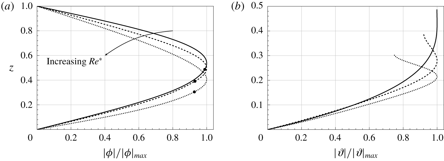
Typical results for  $\unicode[STIX]{x1D719}$ and
 $\unicode[STIX]{x1D717}$ are shown in figure 7, which correspond to flow perturbation and plant deflection respectively.
Magnitudes of unstable eigenmodes  $\unicode[STIX]{x1D719}$ and
 $\unicode[STIX]{x1D717}$ as normalised functions of
 $z$ when
 $h=0.5$,
 $\unicode[STIX]{x1D706}=10^{-1.5}$,
 $C_{Y}/Re^{\ast 2}=10^{-4}$,
 $M_{1}=M_{2}=0.2$,
 $J=10^{-5}$ and
 $k=1$. Results are shown with
 $Re^{\ast }=859$ (solid),
 $2466$ (dashed) and
 $4607$ (dotted). The solid circles on the streamfunctions in (a) indicate their respective canopy height at steady state.

We first note from the behaviour of  $|\unicode[STIX]{x1D719}|$ that, for all cases, the energy of the flow perturbation is localised near the top of the canopy. For slower flows,
 $|\unicode[STIX]{x1D717}|$ increases monotonically in
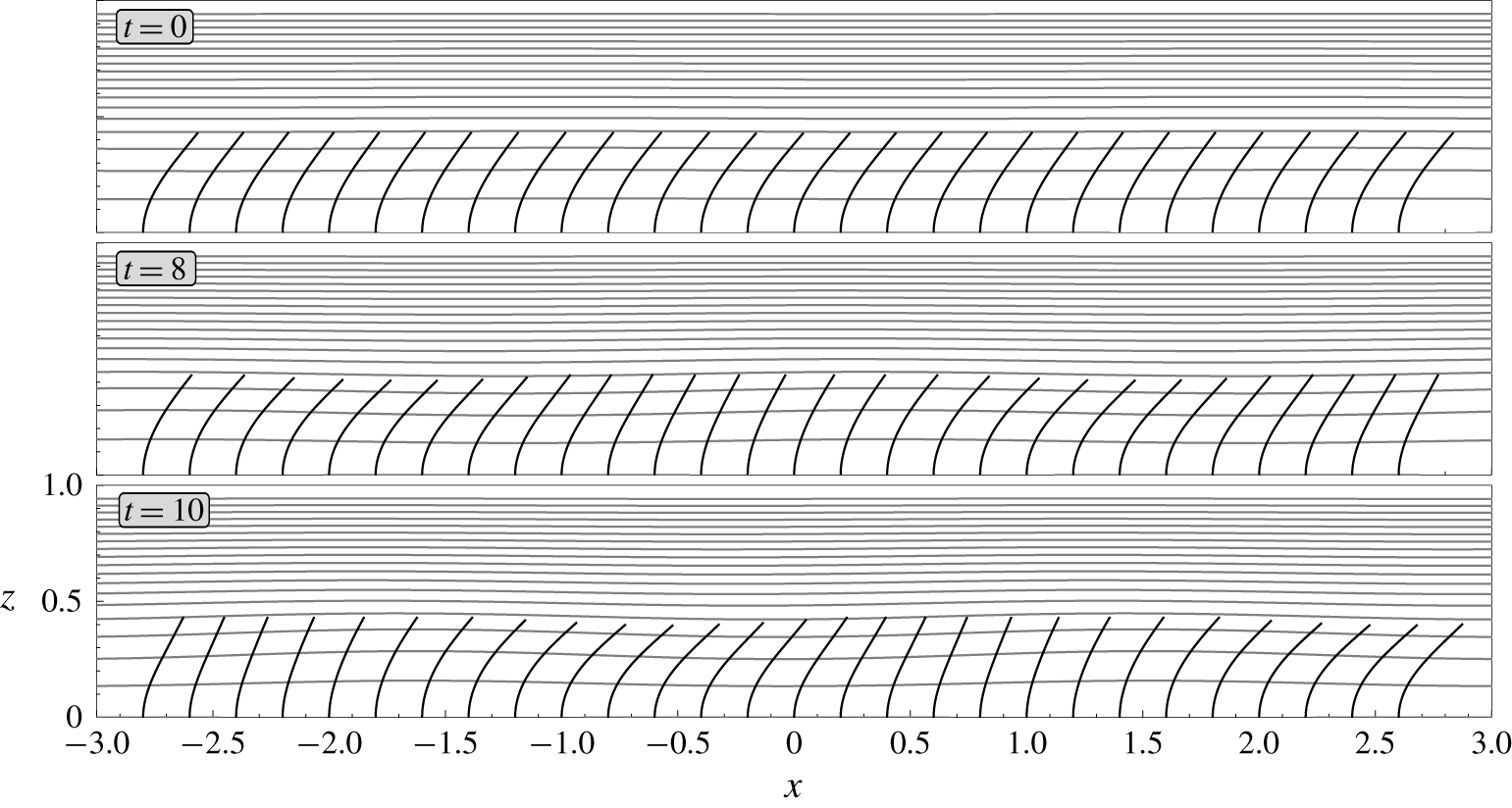
 $z$ so that the perturbations to the deflection angle are also largest at the top of the canopy. Moreover, for faster flows, the largest perturbation to the deflection may be in the middle of the canopy. The temporal evolution of such a mode is illustrated in figure 8.
We can also visualise how the physical configuration evolves in time by perturbing the base flow with a single unstable mode. We plot the streamlines of the flow given by
 $$\begin{eqnarray}\displaystyle \left(\begin{array}{@{}c@{}}u\\ w\end{array}\right)=\left(\begin{array}{@{}c@{}}u^{\ast }(z)\\ 0\end{array}\right)+\unicode[STIX]{x1D6FE}\text{e}^{\text{Re}(\unicode[STIX]{x1D70E})t}\text{Re}\left[\left(\begin{array}{@{}c@{}}\unicode[STIX]{x1D719}^{\prime }(z)\text{e}^{\text{i}[kx+\text{Im}(\unicode[STIX]{x1D70E})t]}\\ -\text{i}k\unicode[STIX]{x1D719}(z)\text{e}^{\text{i}[kx+\text{Im}(\unicode[STIX]{x1D70E})t]}\end{array}\right)\right], & & \displaystyle\end{eqnarray}$$
where  $\unicode[STIX]{x1D6FE}$ is the (arbitrarily chosen) initial amplitude.
In figure 8, we present the perturbed configuration at four different instances. The amplitude of the travelling wave grows in time as it convects downstream. If we plot the streamlines in figure 8 without the base flow, we will find closed contours along the top of the canopy corresponding to rolling vortices. Regarding the canopy configuration, plants oscillate synchronously, resembling monami. In particular, at later times, we see that when the deflection near the base of the canopy is increased, the canopy becomes more aligned with the flow. The drag higher up the canopy is then reduced. As a result, the deflection angle higher up the canopy is also reduced. We highlight that our flexible-canopy model can capture the streamwise variation of the canopy height and the local angle of deflection for each plant.
Temporal evolution of a steady unidirectional base flow in the domain due to the growth of a single unstable eigenmode. The configuration of individual plants in the canopy are represented by black solid lines (to scale) along the bottom of the domain with streamlines in grey. For the eigenmode,  $\unicode[STIX]{x1D719}$ and
 $\unicode[STIX]{x1D717}$ are rescaled by
 $|\unicode[STIX]{x1D719}|_{max}$ before we impose an initial amplitude of
 $\unicode[STIX]{x1D6FE}=10^{-3}$ in (6.2). Shown is the case where
 $h=0.5$,
 $Re^{\ast }=2936$,
 $\unicode[STIX]{x1D706}=10^{-1}$,
 $C_{Y}/Re^{\ast 2}=10^{-4}$,
 $M_{1}=M_{2}=0.2$,
 $J=10^{-5}$ and
 $k=2$.

6.2 Stability of flows for sparse and dense canopies
Analogous to the analysis on the base flows in § 3.2, we can gain some insight into the stability of the system by considering the asymptotic limits of small and large canopy densities. In the dense-canopy limit, we expect the perturbations to be less sensitive to plant flexibility: there will be less flow in the canopy, which also leads to less deformation. In the opposite limit, we expect a sparse canopy to have limited influence on the macroscopic flow, irrespective of the physical properties of individual plants.
6.2.1 Stability of flows for sparse canopies
In the limit where the canopy is sparse, in the sense that  $Re^{\ast }\unicode[STIX]{x1D706},\,Re^{\ast 2}\unicode[STIX]{x1D706}\ll 1$, we know from § 3.2 that
 $u_{0}\sim 1$ and the momentum sink in (4.12a) becomes negligible. Since the perturbations of the beams are then decoupled from the fluid, we can approximate the eigenvalues of the full problem by only solving the Orr–Sommerfeld equation
 $$\begin{eqnarray}\frac{1}{Re^{\ast }}(\unicode[STIX]{x1D719}^{\prime \prime \prime \prime }-2k^{2}\unicode[STIX]{x1D719}^{\prime \prime }+k^{4}\unicode[STIX]{x1D719})=(\unicode[STIX]{x1D70E}+\text{i}k)(\unicode[STIX]{x1D719}^{\prime \prime }-k^{2}\unicode[STIX]{x1D719}).\end{eqnarray}$$
We can solve this equation analytically in the limit when  $J=Fr/Re^{\ast }\rightarrow 0$, for which
 $$\begin{eqnarray}\unicode[STIX]{x1D719}(0)=0,\quad \unicode[STIX]{x1D719}(1)=0,\quad \unicode[STIX]{x1D719}^{\prime \prime }(0)=0,\quad \unicode[STIX]{x1D719}^{\prime \prime }(1)=0\end{eqnarray}$$
to give
 $$\begin{eqnarray}\unicode[STIX]{x1D70E}(k)=-\frac{1}{Re^{\ast }}(k^{2}+n^{2}\unicode[STIX]{x03C0}^{2})-k\text{i},\end{eqnarray}$$
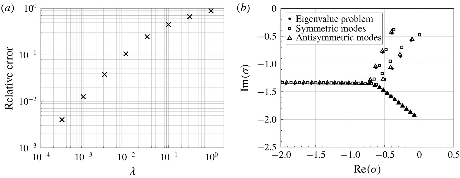
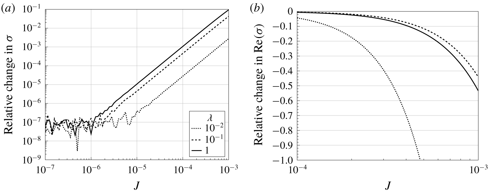
where  $n\in \mathbb{N}$. Thus, a uniform flow in this limit is globally stable. As a check on both our asymptotic and numerical results, we compare the leading eigenvalue with that of the full numerical solution in figure 9(a).
In the distinguished limit in which  $Re^{\ast }\unicode[STIX]{x1D706}\ll 1$ with
 $Re^{\ast 2}\unicode[STIX]{x1D706}$ being
 $O(1)$, we can apply the approximations for the velocity profile in § 3.2 for rigid canopies and rewrite the eigenvalue problem as a universal problem
 $$\begin{eqnarray}\unicode[STIX]{x1D719}^{\prime \prime \prime \prime }-2k^{2}\unicode[STIX]{x1D719}^{\prime \prime }+k^{4}\unicode[STIX]{x1D719}=(\unicode[STIX]{x1D70E}_{new}+\text{i}kRe^{\ast 2}\unicode[STIX]{x1D706}\tilde{u} )(\unicode[STIX]{x1D719}^{\prime \prime }-k^{2}\unicode[STIX]{x1D719})-\text{i}kRe^{\ast 2}\unicode[STIX]{x1D706}\tilde{u} ^{\prime \prime }\unicode[STIX]{x1D719}+O(Re^{\ast }\unicode[STIX]{x1D706}),\end{eqnarray}$$
with  $\tilde{u}$ given by (3.6) and
 $\unicode[STIX]{x1D70E}_{new}=Re^{\ast }(\unicode[STIX]{x1D70E}+k\text{i})$, where
 $\unicode[STIX]{x1D719}$ satisfies the simplified boundary conditions (6.4) for small
 $J$. Furthermore, note from (6.6) that the eigenfunctions are determined via the single parameter,
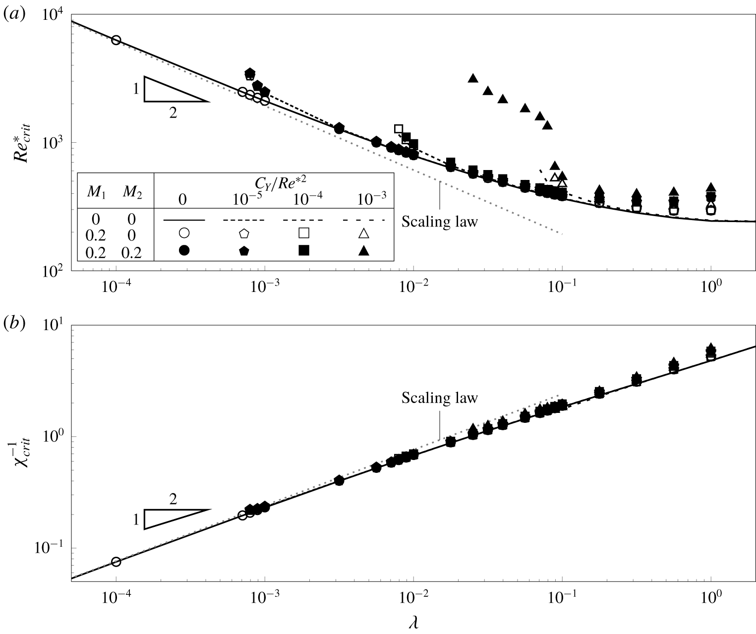
 $Re^{\ast 2}\unicode[STIX]{x1D706}$. In fact, this determines the critical Reynolds number for instability when the canopy is sparse, as verified in § 7.
Comparison between the spectrum of the eigenvalue problem (4.12) and some reduced problems for  $h=0.5$,
 $C_{Y}/Re^{\ast 2}=10^{-4}$,
 $M_{1}=M_{2}=0$,
 $J=10^{-5}$ and
 $k=2$. (a) Relative error between the least stable eigenvalue of the eigenvalue problem and the sparse-canopy approximation (6.5) for different values of
 $\unicode[STIX]{x1D706}$ when
 $Re^{\ast }=200$. (b) Positions of the most unstable eigenvalues for the full problem and the corresponding symmetric and antisymmetric modes of the classic Orr–Sommerfeld problem (6.7) when
 $Re^{\ast }=2\times 10^{4}$,
 $\unicode[STIX]{x1D706}=10^{5}$.

6.2.2 Stability of flows for dense canopies
Recall from our dense-canopy analysis in § 3.2.2 that, in the limit  $\unicode[STIX]{x1D706}\rightarrow \infty$, the flow inside the canopy satisfies
 $u^{\ast }=O(\unicode[STIX]{x1D706}^{-1/2})$ from (3.8). Moreover, the flow above the canopy is parabolic and given by (3.9) and (3.12). Thus, in the limit where
 $J\rightarrow 0$, we should recover the eigenvalues of the classic Orr–Sommerfeld problem for a plane Poiseuille flow between
 $[h,2-h]$ with
 $u_{0}=0$ at
 $z=h$ (the channel bottom) and
 $u_{0}=1$ at
 $z=1$ (the flow centreline). Mathematically, this gives (compare with Drazin & Reid Reference Drazin and Reid1982)
 $$\begin{eqnarray}\frac{1}{Re^{\ast }}(\unicode[STIX]{x1D719}^{\prime \prime \prime \prime }-2k^{2}\unicode[STIX]{x1D719}^{\prime \prime }+k^{4}\unicode[STIX]{x1D719})=(\unicode[STIX]{x1D70E}+\text{i}ku_{0})(\unicode[STIX]{x1D719}^{\prime \prime }-k^{2}\unicode[STIX]{x1D719})-\text{i}ku_{0}^{\prime \prime }\unicode[STIX]{x1D719},\end{eqnarray}$$
with
 $$\begin{eqnarray}\unicode[STIX]{x1D719}(h)=0,\quad \unicode[STIX]{x1D719}^{\prime }(h)=0,\quad \unicode[STIX]{x1D719}(2-h)=0,\quad \unicode[STIX]{x1D719}^{\prime }(2-h)=0.\end{eqnarray}$$
Note that the above problem has two types of modes: symmetric and antisymmetric modes (Chapman Reference Chapman2002). Since we have imposed the simplified shear-free condition at  $z=1$, eigenmodes of our problem (4.12) in this limit will only correspond to the antisymmetric modes of the classic problem (6.7), as seen in figure 9(b). These modes are always stable (Orszag Reference Orszag1971). Therefore, our problem is also linearly stable in the dense-canopy limit.
7 Critical conditions for the onset of instability
In the previous section, we have seen that the system is linearly stable when the canopy is infinitely sparse or dense. However, we found that unstable modes exist for intermediate canopy densities. Therefore, it is natural for us to investigate the critical conditions for the onset of instability. The intention of this section is to describe the global stability structure of the perturbed system. This leads up to the main results of this work on the role of flexibility, inertia, and shear in flows through vegetation.
7.1 Evolution of the neutral curve
Our main objective is to observe the change in the neutral stability curves as four key parameters are changed: the flexibility  $C_{Y}/Re^{\ast 2}$; canopy density
 $\unicode[STIX]{x1D706}$; added mass
 $M_{1}$; and beam inertia and virtual buoyancy
 $M_{2}$. For each choice of these four parameters, our numerical scheme is used to generate heat maps of
 $\text{Re}(\unicode[STIX]{x1D70E})$ in the
 $(Re^{\ast },k)$-plane. For example, values of
 $\text{Re}(\unicode[STIX]{x1D70E})$ at fixed values of
 $M_{1}=0.2$ and
 $M_{2}=0.2$ are represented by the greyscale colours of insets in figure 10(b–f). Then, the key contour is given by the neutral stability curve,
 $\operatorname{Re}(\unicode[STIX]{x1D70E})=0$, and is shown solid in these insets. In addition, simulations are performed by varying
 $M_{1}$ and
 $M_{2}$; these give the shifted neutral stability curves and are plotted with other line styles. We shall discuss these elements in § 7.1.1.
The main figure (a) shows the  $(C_{Y}/Re^{\ast 2},\unicode[STIX]{x1D706})$-solution space for the eigenvalue problem (4.12) for
 $M_{2}=0$. The shaded region indicates where perturbations of the base state are stable, and lies below the critical curve for instability,
 $\unicode[STIX]{x1D706}=\unicode[STIX]{x1D706}_{c}$. Hollow markers are numerically determined solutions with
 $M_{1}=0$ (triangles) and
 $M_{1}=0.2$ (squares). The five insets (b) through (f) show heat maps of
 $\text{Re}(\unicode[STIX]{x1D70E})$ in the
 $(Re^{\ast },k)$-plane. In all heat maps, colours correspond to values of
 $\text{Re}(\unicode[STIX]{x1D70E})$ ranging from
 $-0.2$ (black) to
 $0.2$ (white) specifically for
 $M_{1}=M_{2}=0.2$; areas that have not been swept are hatched. The neutral stability curve,
 $\text{Re}(\unicode[STIX]{x1D70E})=0$, for
 $M_{1}=M_{2}=0.2$ is given by a solid line. Other line styles are used to indicate neutral curves with
 $M_{1}=0.2$,
 $M_{2}=0$ (dashed),
 $M_{1}=M_{2}=0$ (dotted) and the decoupled model in § 7.1.2 (dash-dotted).

Once the heat maps are generated for a range of parameters, the results are visualised in the  $(C_{Y}/Re^{\ast 2},\unicode[STIX]{x1D706})$-plane, as shown in figure 10(a). Here, solutions are either classified as stable or unstable (corresponding to a non-trivial neutral stability curve).
Before proceeding further, let us make two basic observations. Firstly, for a given choice of the four parameters, if an instability exists, then the base state will initially become unstable at a critical wavenumber,  $k$, that is
 $O(1)$. Secondly, although not shown in the figure, all of the unstable modes have
 $\text{Im}(\unicode[STIX]{x1D70E})<0$, with
 $|\text{Im}(\unicode[STIX]{x1D70E})|$ increasing nonlinearly with
 $k$ for any given
 $Re^{\ast }$. This corresponds to the instabilities being convective downstream and dispersive, and is in agreement with the predictions by Singh et al. (Reference Singh, Bandi, Mahadevan and Mandre2016) and Luminari et al. (Reference Luminari, Airiau and Bottaro2016) on flows through rigid canopies.
7.1.1 Variations due to inertia
We now discuss how the neutral stability curves shown in figure 10(b–f) vary as a function of the four parameters. We make the following observations:
(i) For fixed flexibility,
$C_{Y}/Re^{\ast 2}$, added mass, $M_{1}$, beam inertia, $M_{2}$, and decreasing canopy density, $\unicode[STIX]{x1D706}$, i.e. as we transition from (b) to (c) to (d) in figure 10(a), the topology of the neutral curves change: the area enclosed by the neutral curves shown in the insets tends to zero and the system becomes globally stable.(ii) Thus, for each
$M_{1}$, $M_{2}$ there exists a critical curve (7.1)in the$$\begin{eqnarray}\unicode[STIX]{x1D706}=\unicode[STIX]{x1D706}_{c}(C_{Y}/Re^{\ast 2};M_{1},M_{2}),\end{eqnarray}$$$(C_{Y}/Re^{\ast 2},\unicode[STIX]{x1D706})$-plane that separates the two possibilities – globally stable for all $Re^{\ast }$, or unstable for some $Re^{\ast }$.(iii) This curve,
$\unicode[STIX]{x1D706}=\unicode[STIX]{x1D706}_{c}$, is shown in figure 10(a), with points on this critical curve for $(M_{1},M_{2})=(0,0)$ and $(0.2,0)$ shown as triangles and squares respectively (and joined by dotted lines). Our numerical results suggest that the curve for $M_{1}=0$ lies below that for $M_{1}=0.2$ for $C_{Y}/Re^{\ast 2}=10^{-3}$. We will return to such features in § 7.4 where we interpret the existence of $\unicode[STIX]{x1D706}_{c}$ in terms of shear.(iv) This trend of a shrinking domain of instability also occurs for fixed
$\unicode[STIX]{x1D706}$ and for increasing $C_{Y}/Re^{\ast 2}$ i.e. as we transition from (b) to (e) to (f) in figure 10(a).





(a) Critical Reynolds number,  $Re_{crit}^{\ast }$, and (b) the corresponding collapsed data for the critical shear at the top of the canopy,
 $\unicode[STIX]{x1D712}_{crit}^{-1}$, for flows with different canopy densities. Shown is the case where
 $h=0.5$ and
 $J=10^{-5}$. Symbols and black lines are used to indicate plant flexibilities,
 $C_{Y}/Re^{\ast 2}$, and values of
 $M_{1}$ and
 $M_{2}$, as stated in the legend of (a). The grey dotted lines indicate the scaling predictions for sparse canopies (cf. discussion following (6.6)).

In the case of cylindrical beams, a non-zero but small beam inertia (or virtual buoyancy),  $M_{2}$, has the effect of shifting the neutral stability curve slightly to the right. Furthermore, as we increase the beam flexibility,
 $C_{Y}/Re^{\ast 2}$, from (b) to (e) to (f) in figure 10, it seems as though the neutral curve for
 $M_{2}=0.2$ may not close and vanish in the same way as the neutral curve for
 $M_{2}=0$, so that there may always be an unstable mode at that canopy density. To really check this would require moving to even higher flexibilities. However, because the beams are bent close to horizontal at such high flexibilities and speeds, the validity of the model in this regime is not clear, in addition to the numerical challenges it poses.
7.1.2 A decoupled model where perturbations of the canopy are ignored
Despite the complexity of the solution space presented above, it appears that some qualitative behaviour of the neutral stability curves shown in figure 10 can be understood through hydrodynamical effects. To this end, we investigate the effect of considering only perturbations in the flow, effectively treating the canopy as rigid and fixed in its deflected position due to the base flow. This is equivalent to setting the perturbations on the canopy,  $\unicode[STIX]{x1D717}$, and stresses,
 ${\mathcal{T}}_{1,3}$, to zero in (4.11) and solving the single equation (4.12a) for
 $\unicode[STIX]{x1D719}$. Once this is done, the neutral stability curves for this decoupled problem are derived.
We return to the heat maps shown in the insets (b)–(f) of figure 10, where the neutral stability curves of the decoupled system are shown as dash-dotted, in contrast to those of the full problem shown as solid. Note that, consistent with the analysis in § 3.3, when the canopy is dense or the plants are stiff, we would expect agreement between the two models. As either density,  $\unicode[STIX]{x1D706}$, decreases or plant flexibility,
 $C_{Y}/Re^{\ast 2}$ increases, the effects of the fluid–plant coupling can then be seen by noticing the growing separation between the curves.
7.2 Behaviour of the critical Reynolds number
We saw in figure 10 that if there are any unstable modes in the parameter space, then for every neutral curve there exists a minimum value,  $Re^{\ast }=Re_{crit}^{\ast }$, such that flows will be first unstable if
 $Re^{\ast }>Re_{crit}^{\ast }$. Therefore, it is natural for us to analyse the behaviour of
 $Re_{crit}^{\ast }$ as a function of the other parameters, i.e.
 $$\begin{eqnarray}Re_{crit}^{\ast }=Re_{crit}^{\ast }(\unicode[STIX]{x1D706},C_{Y},M_{1},M_{2}).\end{eqnarray}$$
For fixed flexibility  $C_{Y}/Re^{\ast 2}$, we observe in figure 11(a) there is a critical density
 $\unicode[STIX]{x1D706}$ at which
 $Re_{crit}^{\ast }$ is minimum. Higher or lower canopy densities are both more stable, in that they lead to a higher
 $Re_{crit}^{\ast }$. This non-monotonic behaviour can be understood through the asymptotic analysis of § 6.2. In particular, as the canopy density decreases to zero or increases to infinity, the base flow is globally stable. For small
 $\unicode[STIX]{x1D706}$ the system is stable for
 $\unicode[STIX]{x1D706}<\unicode[STIX]{x1D706}_{c}$ at which point
 $Re_{crit}^{\ast }\rightarrow \infty$.
For all values of  $M_{1}$,
 $M_{2}$ and
 $\unicode[STIX]{x1D706}$ the critical Reynolds number
 $Re_{crit}^{\ast }$ increases with flexibility, with the effect more pronounced for low canopy densities. Finally, it always requires a higher Reynolds number to destabilise flows through the same canopy when we account for inertia.
7.3 Behaviour of the critical shear
In the previous discussion, we have sought to understand the effects of plant flexibility, canopy density and inertia on the critical value of  $Re^{\ast }$ separating stable and unstable flows. However, there are interesting insights once this is viewed in terms of shear.
As mentioned in the introduction, it is known from turbulence statistics that canopy-scale instabilities are generated by shear of the flow along the top of the canopy (Raupach et al. Reference Raupach, Finnigan and Brunet1996; Finnigan Reference Finnigan2000). However, previous stability analyses did not account for the free surface, canopy perturbations or inertial effects such as added mass and virtual buoyancy. We would like to understand whether these additional physical effects affect the shearing mechanism.
A simple measurement for shear at a given depth is to consider its reciprocal – the (dimensionless) Navier slip length. In particular, suppose we let  $\unicode[STIX]{x1D712}$ be this slip length at steady state at the top of the canopy
 $z=z_{0}^{\ast }$. We then define
 $$\begin{eqnarray}\unicode[STIX]{x1D712}=\frac{u^{\ast }(z_{0}^{\ast })}{{u^{\ast }}^{\prime }(z_{0}^{\ast })}.\end{eqnarray}$$
For every flow that is marginally stable, we can quantify the critical shear with  $\unicode[STIX]{x1D712}_{crit}^{-1}$.
We observe from figure 11(b) that for any given canopy density:
(i) the critical shear,
$\unicode[STIX]{x1D712}_{crit}^{-1}$, increases monotonically with $\unicode[STIX]{x1D706}$;(ii) the critical shear,
$\unicode[STIX]{x1D712}_{crit}^{-1}$, is nearly identical across different plant flexibilities when we neglect inertial effects – even when $Re_{crit}^{\ast }$ and the configuration of the canopies (at their base states) are distinct;(iii) although there is a significant collapse in the data compared to the same plot for
$Re_{crit}^{\ast }$, there is a spread for $\unicode[STIX]{x1D712}_{crit}^{-1}$ for different flexibilities. This spread increases with increasing $M_{1}$ and $M_{2}$ for any given $\unicode[STIX]{x1D706}$.


The significant collapse in the data suggests that shear at the top of the canopy remains the relevant criterion in determining the stability of steady unidirectional flows. There is a slight spread when inertial effects are prominent, with the critical shear being larger for non-zero added mass and beam inertia. Nevertheless, the collapse of the data for different plant flexibilities means the simplified model, where inertia is neglected,  $M_{1}=M_{2}=0$, can still provide a useful reference value for the critical shear.
Many features of figure 11(b) in the limits of dense or spare canopies are explained by the asymptotic analysis of § 6.2. For instance, in the case of sparse rigid canopies, we previously found that  $Re_{crit}^{\ast }=O(\unicode[STIX]{x1D706}^{-1/2})$ (cf. figure 11a). Thus, in combination with (7.3),
 $\unicode[STIX]{x1D712}_{crit}=O(\unicode[STIX]{x1D706}^{-1/2})$ as
 $\unicode[STIX]{x1D706}\rightarrow 0$; this is shown dotted in figure 11(b).
7.4 Summary of the physical mechanisms
In § 7, we have sought to study the key conditions for the onset of instabilities. Our primary conclusion is that instabilities are induced by sufficient shear along the top of the canopy, and this is accompanied by non-monotonic behaviour of the critical Reynolds number,  $Re_{crit}^{\ast }$, with canopy density,
 $\unicode[STIX]{x1D706}$.
We have found that if  $\unicode[STIX]{x1D706}>\unicode[STIX]{x1D706}_{c}$ as given in (7.1) the base flow can be unstable for sufficiently large Reynolds numbers. In such cases, let us write
 $\unicode[STIX]{x1D6EC}=\unicode[STIX]{x1D6EC}(C_{Y}/Re^{\ast 2},M_{1},M_{2})$ for the canopy density corresponding to the minimum
 $Re_{crit}^{\ast }$ (the turning point in figure 11a). For canopies with
 $\unicode[STIX]{x1D706}>\unicode[STIX]{x1D6EC}$, the shear threshold is greater and therefore a faster flow is required for instability. On the other hand for
 $\unicode[STIX]{x1D706}<\unicode[STIX]{x1D6EC}$, although the shear threshold is lower, a faster flow is required to generate this shear; this is due to the reduced momentum loss on account of reconfiguration, which can also be achieved by increasing flexibility,
 $C_{Y}/Re^{\ast 2}$. However, if
 $\unicode[STIX]{x1D706}<\unicode[STIX]{x1D706}_{c}$, this shear threshold will never be reached, irrespective of the flow speed. This differentiates flexible canopies from rigid canopies, where drag monotonically increases with flow speed (cf. figure 6b) and hence,
 $\unicode[STIX]{x1D706}_{c}=0$. Finally, for both cylindrical beams and blades, added mass increases the shear threshold, which stabilises the flow.
8 Conclusions
In this work, we have considered free-surface flow through a deformable vegetative region, and have attempted to analyse conditions for the onset of instabilities. We have studied the roles of various physical factors in triggering or suppressing a monami. Our results have allowed us to confirm that shear at the top of the canopy can be considered as a primary mechanism for instability, and this indeed agrees with previous analyses for the specific case of rigid vegetation. Our study, however, extends this conclusion by exploring vegetative flows with additional effects such as canopy flexibility and inertia.
Our results suggest that flexibility affects the flow stability in two distinct ways. Firstly, compared to rigid-canopy flows, flexible-canopy flows are more stable by having less drag due to plant reconfiguration in the underlying base state. In particular, if the canopy density is below a critical threshold, the flow will not be able to generate sufficient shear to trigger an instability, irrespective of the Reynolds number. Secondly, by decoupling the fluid perturbations from the canopy perturbations, we found that for a given base flow, flexibility can encourage instability. Furthermore, by studying the growth of a single unstable eigenmode, our model can also capture the temporal evolution of monami.
9 Discussion
One important conclusion from the present study is that the shear at the top of the canopy remains the dominant factor in determining the stability of a flow. Thus, one interesting question that follows is whether there may be particular flow regimes where more involved models are required, and for which the central mechanism for instability may be different. As a particular example, we highlight the review by Nepf (Reference Nepf2012), who notes that as the canopy becomes increasingly sparse, the flow transitions from a mixing-layer-like flow to a boundary-layer flow. In our current model, we have neglected the effects of bed shear, and this hints at the need for a model for which the sparse-canopy limit can be more accurately captured.
Which length scales might be involved in a more complete model? An important avenue for progress is the consideration of a more complete turbulence model. Note that we analysed flow stability using a single mixing length at the top of the canopy (7.3) and our constant eddy viscosity closure model can be interpreted as effectively averaging the various length scales involved. However, in limits of small or large elasticity/density, it is unclear whether it may be necessary to consider a better closure model in order to capture disparate length scales in the flow.
Firstly, the bed can be rough in reality and the boundary layer along it may contribute one length scale. Secondly, there is an element scale inside the canopy, which is determined by the wakes of individual plants. Thirdly, for deeply submerged canopies ( $h\ll 1$), the turbulence that is generated far below is expected to be negligible far above. Thus, there is a length scale that is determined by the decay of the canopy-scale vortices. Finally, in a more general setting where the pressure gradient of the flow is not maintained, there will also be a decay length scale for the flow. A more detailed description of the different length scales can be found in Marion et al. (Reference Marion, Nikora, Puijalon, Bouma, Koll, Ballio, Tait, Zaramella, Sukhodolov and O’Hare2014).
We envision that a more refined model will capture a number of these length scales. However, in order to implement such a scheme, we require a better understanding of the importance of these length scales. Moreover, we would hope to determine these scales as part of the model, rather than verified a posteriori from given parameters (see discussion in Poggi et al. (Reference Poggi, Porporato, Ridolfi, Albertson and Katul2004)).
What if the base flow is oscillatory? In this work, we considered a regime where the flow is current dominated. There is also a great deal of interest in the study of oscillatory flows through vegetation. Compared to unidirectional flows of the same magnitude, oscillatory flows can potentially have higher in-canopy flow velocities (Lowe, Koseff & Monismith Reference Lowe, Koseff and Monismith2005) and vegetation can also move out of phase with the waves (Gijón Mancheño Reference Gijón Mancheño2016). A natural extension of our work is to utilise our coupled model to analyse such flows. In particular, it is important to understand how momentum loss can be affected by the wave height (Bradley & Houser Reference Bradley and Houser2009), wave frequency (Mattis et al. Reference Mattis, Kees, Wei, Dimakopoulos and Dawson2019) and the presence of a current (Zeller et al. Reference Zeller, Weitzman, Abbett, Zarama, Fringer and Koseff2014; Lei & Nepf Reference Lei and Nepf2019). An ultimate application of interest is to predict wave attenuation over a long distance via flexible vegetation (Mendez & Losada Reference Mendez and Losada2004; Mei et al. Reference Mei, Chan, Liu, Huang and Zhang2011; Mei, Chan & Liu Reference Mei, Chan and Liu2014; Wang, Guo & Mei Reference Wang, Guo and Mei2015).
Acknowledgement
This publication is based on work partially supported by the EPSRC Centre for Doctoral Training in Industrially Focused Mathematical Modelling (EP/L015803/1) in collaboration with HR Wallingford and US Army Engineer Research and Development Center. We would like to thank A. Dimakopoulos from HR Wallingford and C. Kees from US Army ERDC for their important contributions. We are also grateful to I. Hewitt, P. Howell and D. Vella for insightful discussions, and note as well the many helpful suggestions by the anonymous reviewers that impacted this manuscript.
Declaration of interests
The authors report no conflict of interest.
Appendix A. Momentum sinks in the eigenvalue problem
In this appendix, we provide the expressions of the momentum sinks given in the Orr–Sommerfeld equation for  $\unicode[STIX]{x1D719}$ (4.12a) and the perturbed beam equations they satisfy. The momentum sinks
 $S_{c}$ and
 $S_{s}$ can be written in the form
 $$\begin{eqnarray}\displaystyle {\mathcal{S}}_{c}(z) & = & \displaystyle u^{\ast }\cos \unicode[STIX]{x1D703}^{\ast }\left[\cos \unicode[STIX]{x1D703}^{\ast }\left(\unicode[STIX]{x1D719}^{\prime }-\unicode[STIX]{x1D70E}{\mathcal{A}}\right)-\sin \unicode[STIX]{x1D703}^{\ast }\left(u^{\ast }\unicode[STIX]{x1D717}-\text{i}k\unicode[STIX]{x1D719}+\unicode[STIX]{x1D70E}{\mathcal{B}}\right)\right]\nonumber\\ \displaystyle & & \displaystyle +\,M_{1}\left[\left(\unicode[STIX]{x1D70E}\unicode[STIX]{x1D719}^{\prime }-\unicode[STIX]{x1D70E}^{2}{\mathcal{A}}\right)\cos \unicode[STIX]{x1D703}^{\ast }+\left(\text{i}k\unicode[STIX]{x1D70E}\unicode[STIX]{x1D719}-\unicode[STIX]{x1D70E}^{2}{\mathcal{B}}\right)\sin \unicode[STIX]{x1D703}^{\ast }\right]+M_{2}\sec \unicode[STIX]{x1D703}^{\ast }\unicode[STIX]{x1D70E}\unicode[STIX]{x1D719}^{\prime },\end{eqnarray}$$
 $$\begin{eqnarray}\displaystyle {\mathcal{S}}_{s}(z) & = & \displaystyle {\textstyle \frac{1}{2}}u^{\ast 2}\unicode[STIX]{x1D717}+u^{\ast }\sin \unicode[STIX]{x1D703}^{\ast }\left[\cos \unicode[STIX]{x1D703}^{\ast }\left(\unicode[STIX]{x1D719}^{\prime }-\unicode[STIX]{x1D70E}{\mathcal{A}}\right)-\sin \unicode[STIX]{x1D703}^{\ast }\left(u^{\ast }\unicode[STIX]{x1D717}-\text{i}k\unicode[STIX]{x1D719}+\unicode[STIX]{x1D70E}{\mathcal{B}}\right)\right]\nonumber\\ \displaystyle & & \displaystyle +\,M_{1}\tan \unicode[STIX]{x1D703}^{\ast }\left[\left(\unicode[STIX]{x1D70E}\unicode[STIX]{x1D719}^{\prime }-\unicode[STIX]{x1D70E}^{2}{\mathcal{A}}\right)\cos \unicode[STIX]{x1D703}^{\ast }+\left(\text{i}k\unicode[STIX]{x1D70E}\unicode[STIX]{x1D719}-\unicode[STIX]{x1D70E}^{2}{\mathcal{B}}\right)\sin \unicode[STIX]{x1D703}^{\ast }\right]+M_{2}\sec \unicode[STIX]{x1D703}^{\ast }\text{i}k\unicode[STIX]{x1D70E}\unicode[STIX]{x1D719},\nonumber\\ \displaystyle & & \displaystyle\end{eqnarray}$$
with
 $$\begin{eqnarray}\displaystyle & \displaystyle {\mathcal{A}}(z)=\int _{0}^{z}\unicode[STIX]{x1D717}-{\mathcal{C}}\cos \unicode[STIX]{x1D703}^{\ast }{\unicode[STIX]{x1D703}^{\ast }}^{\prime }\,\text{d}\overline{z}, & \displaystyle\end{eqnarray}$$
 $$\begin{eqnarray}\displaystyle & \displaystyle {\mathcal{B}}(z)=\int _{0}^{z}\tan \unicode[STIX]{x1D703}^{\ast }\left(\unicode[STIX]{x1D717}-{\mathcal{C}}\cos \unicode[STIX]{x1D703}^{\ast }{\unicode[STIX]{x1D703}^{\ast }}^{\prime }\right)\,\text{d}\overline{z}. & \displaystyle\end{eqnarray}$$
The expression for  ${\mathcal{C}}$ is given in (4.12b). The equations which the dependent variables above satisfy are
 $$\begin{eqnarray}\displaystyle & \displaystyle {\mathcal{T}}_{1}^{\prime }(z)=-{\mathcal{S}}_{c}+M_{2}\sec \unicode[STIX]{x1D703}^{\ast }\unicode[STIX]{x1D70E}^{2}{\mathcal{A}}, & \displaystyle\end{eqnarray}$$
 $$\begin{eqnarray}\displaystyle & \displaystyle {\mathcal{T}}_{3}^{\prime }(z)={\mathcal{S}}_{s}-M_{2}\sec \unicode[STIX]{x1D703}^{\ast }\unicode[STIX]{x1D70E}^{2}{\mathcal{B}}, & \displaystyle\end{eqnarray}$$
 $$\begin{eqnarray}\displaystyle \unicode[STIX]{x1D717}^{\prime \prime }(z) & = & \displaystyle C_{Y}\sec \unicode[STIX]{x1D703}^{\ast }\left[\tan \unicode[STIX]{x1D703}^{\ast }{\mathcal{T}}_{3}+T_{3}^{\ast }(2\sec ^{2}\unicode[STIX]{x1D703}^{\ast }-1)\unicode[STIX]{x1D717}-{\mathcal{T}}_{1}-T_{1}^{\ast }\tan \unicode[STIX]{x1D703}^{\ast }\unicode[STIX]{x1D717}\right]\nonumber\\ \displaystyle & & \displaystyle +\,2\tan \unicode[STIX]{x1D703}^{\ast }{\unicode[STIX]{x1D703}^{\ast }}^{\prime }\unicode[STIX]{x1D717}^{\prime }+\sec ^{2}\unicode[STIX]{x1D703}^{\ast }\left({\unicode[STIX]{x1D703}^{\ast }}^{\prime }\right)^{2}\unicode[STIX]{x1D717}.\end{eqnarray}$$
We solve the differential equations above alongside the Orr–Sommerfeld equation with the boundary conditions (4.12c)–(4.12g) and the jump conditions (4.12h)–(4.12i).
Appendix B. A discussion on inertia and the Froude number
In this appendix, we discuss the significance of inertia and gravity in our problem. Mathematically, they are quantified in relation to other physical effects by the dimensionless parameters  $M_{1}$,
 $M_{2}$ and
 $Fr$ (cf. table 2).
B.1 Magnitudes of $M_{1}$ and $M_{2}$


For cylindrical beams, the cross-sectional mass per unit length  $m=\unicode[STIX]{x1D70C}\unicode[STIX]{x03C0}b^{2}/4$. With the drag coefficient
 $C_{D}$ being
 $O(1)$,
 $M_{1,2}=O(b/H)\ll 1$ i.e. the aspect ratio of the beam provided that
 $h=l/H$ is
 $O(1)$. The same calculation for blades with thickness
 $\tilde{b}$ gives
 $M_{1}=O(b/H)\ll 1$, but
 $M_{2}=O(\tilde{b}/H)\ll b/H\ll 1$. Although both
 $M_{1}$ and
 $M_{2}$ can be small in relation to drag, inertia can still play a role in beam dynamics for large values of
 $C_{Y}$ (2.18d). In order to highlight the effects of different types of inertia in this problem, we consider non-negligible but representative values of
 $M_{1}$ and
 $M_{2}$ in §§ 6 and 7:
 $M_{1}=M_{2}=0.2$ for cylindrical beams and
 $M_{1}=0.2$,
 $M_{2}=0$ for blades. The approximation for
 $M_{2}=0$ for blades has also been used in the previous study by Leclercq & de Langre (Reference Leclercq and de Langre2018).
Finally, we note that, in order to incorporate the plant dynamics into the Navier–Stokes equations via a momentum sink, we require that both the dimensionless added mass and the volume fraction of the solid at any point in space to be much smaller than unity i.e.  $\unicode[STIX]{x1D706}M_{1},\unicode[STIX]{x1D706}M_{2}\ll 1$.
B.2 Magnitude of $Fr$ and imposing shear-free conditions at $z=1$


As with the Cauchy number, the Froude number also scales with the velocity scale  $U$ (cf. table 2). In order to vary the Reynolds number (by varying
 $U$) while keeping the geometry of the domain fixed, we compare flows that have the same ratio,
 $J$ (6.1). Note that typically,
 $J\ll 1$. For reference, if we take
 $\unicode[STIX]{x1D708}^{\ast }=10^{-4}~\text{m}^{2}~\text{s}^{-1}$ as a representative value for canopy flows (Singh et al. Reference Singh, Bandi, Mahadevan and Mandre2016), then
 $J$ is of the order of
 $10^{-5}$ for a flow of depth
 $H=1$ m.
Previous stability analyses on flows through vegetation have also considered imposing the shear-free condition for the flow at  $z=1$ (Dupont et al. Reference Dupont, Gosselin, Py, de Langre, Hemon and Brunet2010; Singh et al. Reference Singh, Bandi, Mahadevan and Mandre2016). Mathematically, this corresponds to considering the limit when
 $Fr\rightarrow 0$ (i.e.
 $J\rightarrow 0$), in which the full free-surface conditions (4.12d)–(4.12e) reduce to
 $\unicode[STIX]{x1D719}(1)=\unicode[STIX]{x1D719}^{\prime \prime }(1)=0$. Our investigation suggests that this is a reasonable simplification in this model: in figure 12, we demonstrate that, for
 $Re^{\ast }=10^{3}$, a typical Reynolds number in our model for the onset of instabilities (shown in § 7), the change in the spectrum is negligible until
 $J$ reaches values that are beyond our regime of interest. In such cases, the free surface appears to be suppressing instabilities by comparison to a symmetry condition at
 $z=1$. We note that we also get similar trends when we include inertia.
Comparing the most unstable eigenvalue of the problem against the same results calculated using the approximation  $J=0$. Shown is the case where
 $h=0.5$,
 $Re^{\ast }=10^{3}$,
 $C_{Y}/Re^{\ast 2}=10^{-4}$,
 $M_{1}=M_{2}=0$ and
 $k=1$. Line styles are used to indicate canopy densities, as stated in the legend of (a).