

1 Introduction
In the late 1980s, Charles Ragin introduced a new methodology for the social sciences known as qualitative comparative analysis (QCA). The goal, Ragin (Reference Ragin1987, x) writes, “is to identify the unique strengths of case-oriented methods and to formalize them as a general method of qualitative comparison using Boolean algebra.” Among political scientists, the method has made inroads in all subfields, but the largest group of consumers has been qualitative comparativists. A visit to compasss.org, the Internet home of QCA, reveals a bibliography comprising nearly seventy books and hundreds of peer-reviewed articles. Software packages may be downloaded for Stata, R, and UNIX. Aspiring scholars can take QCA training courses around the globe through organizations such as the American Political Science Association (APSA), the European Consortium for Political Research, ICPSR, the International Political Science Association, and the Institute for Qualitative and Multi-Method Research. The leading methodological journal in political science recently published four articles that begin from the premise that QCA is an established methodology and go on to debate some finer points of the method (Thiem Reference Thiem2016, Thiem, Spöhel, and Duşa Reference Thiem, Spöhel and Duşa2016, Rohlfing Reference Rohlfing2018, Schneider Reference Schneider2018).
The growth of QCA remains unabated despite numerous critical assessments (see, e.g., Lieberson (Reference Lieberson2001, Reference Lieberson2004), Seawright (Reference Seawright2005a,Reference Seawrightb), Achen (Reference Achen2005), Dunning (Reference Dunning2012), Brady (Reference Brady2013), Hug (Reference Hug2013), Braumoeller (Reference Braumoeller2015), Krogslund et al. (Reference Krogslund, Choi and Poertner2015), Paine (Reference Paine2016a,Reference Paineb), Munck (Reference Munck2016)). These important contributions focus on problematic assumptions hidden within QCA (Seawright Reference Seawright2005b), incorrect inferences produced by QCA (Hug Reference Hug2013, Braumoeller Reference Braumoeller2015, Krogslund et al. Reference Krogslund, Choi and Poertner2015), and QCA’s lack of distinctiveness relative to conventional statistical methods (Brady Reference Brady2013, Paine Reference Paine2016a,Reference Paineb). None of these articles, however, evaluates the commitments and restrictions researchers must abide by when using QCA, which is based on two-element (0–1) Boolean algebra. Even if QCA can do what its proponents claim (and the articles just cited suggest that it cannot), the method limits how researchers analyze the social world.
Qualitative comparative analysis and its reliance on the two-element Boolean algebra limits scholars in three ways. First, the two-element Boolean algebra restricts what researchers can know and describe about sets and the interactions between sets. I show that the building blocks of statistical analysis—random variables and probability—are based on more general Boolean algebras and allow for richer treatments of sets. Second, I show that the two-element Boolean algebra is a model for propositional logic, which is too weak a language to capture modern social science theories. Third, I show that QCA researchers are restricted to regularity accounts of causation (necessity, sufficiency, and INUS conditions) because these can be modeled with 0–1 Boolean algebra and propositional logic. Counterfactuals, however, cannot be modeled with propositional logic.
Highlighting QCA’s reliance on two-element Boolean algebra and propositional logic brings the weaknesses of QCA into sharp relief. The distinction between QCA and conventional statistics is not a difference between “set-theoretic” methods and what QCA researchers call “non-set-theoretic” methods (Schneider and Wagemann Reference Schneider and Wagemann2012) or the “correlational approach” (Ragin (Reference Ragin2000, Reference Ragin2008)) or “regressional analytic methods (RAMs)” (Thiem, Baumgartner, and Bol Reference Thiem, Baumgartner and Bol2016). Conventional statistics are set-theoretic methods. The distinction between QCA and conventional statistics is also not the difference between a method that captures “the natural language of logic in the qualitative culture” (Goertz and Mahoney Reference Goertz and Mahoney2012, 18) and one that does not. What truly sets QCA apart from conventional statistics is the former’s embrace of the limitations of two-element Boolean algebra and propositional logic. QCA exists in a nether region between qualitative and quantitative research; it exhibits neither the depth of small-
 $n$
qualitative research nor the power of quantitative research.
My discussion unfolds in four parts. In Section 2, I provide a brief introduction to Boolean algebra, and I note that QCA uses only the simplest version of Boolean algebra (two-element Boolean algebra.) In Section 3, I demonstrate the deep connection between Boolean algebras, random variables, and probability. In Section 4, I demonstrate the isomorphism between two-element Boolean algebra and propositional logic and show that propositional logic is too weak to capture social scientific theories. In Section 5, I demonstrate that QCA researchers focus on regularity accounts of causation because such accounts can be modeled with propositional logic.
2 An introduction to Boolean algebras
Claims that “set-theoretic” methods stand apart from conventional statistical analysis generally reference QCA’s use of Boolean algebra. Schneider and Wagemann (Reference Schneider and Wagemann2012, 8), for example, write that QCA makes use of truth tables and the “principles of logic minimization,” which they define as “applying the rules of Boolean algebra” [329]. Thiem, Baumgartner, and Bol (Reference Thiem, Baumgartner and Bol2016, 746) contend that “Boolean algebra establishes the language of CCMs, linear algebra that of RAMs.” We need to know more about Boolean algebras to understand where the intersection with classical statistics lies. In this section, I introduce Boolean algebra and show that the two-element Boolean algebra is a special case.
When people think of Boolean algebra, they often think of sets comprising 0s and 1s, but that is just the simplest example of a (nondegenerate) Boolean algebra. A Boolean algebra is a nonempty set
 $S$
, with two binary operations meet (
 $\vee$
) and join (
 $\wedge$
), a complement (
 $\prime$
), two distinguished elements 0 and 1, and that satisfies the following axiomsFootnote
1
:

Parts of this definition require additional elucidation. A binary operation on a set is a rule that assigns to each ordered pair of elements of the set some element of the set.Footnote
2
So if we use
 $\vee$
and
 $\wedge$
on any subsets of a set, the result is also a member of that set. The complement or negation is a unary operator, which means that it is a rule that assigns an element of the set some element of the set.Footnote
3
If we use
 $\prime$
on any subset of a set, the result is also a member of that set. Finally, a distinguished element is an identity element for a binary operation. That is, we need an element
 $e$
such that
 $p\wedge e=p$
and
 $p\vee e=p$
, and 0 and 1 are those two elements.
Nothing that we have said so far demands that a Boolean algebra includes only 0s and 1s. All we need to form a Boolean algebra are two binary operations, a unary operator, and two elements that satisfy the identity requirements (and meet the axioms). Consider, for instance, the set
 $X=\{1,2,3,6\}$
.
 $X$
along with the following operations
-
∙
 $a\vee b=lcm(a,b),\,\forall \;a,b\in X$
,
-
∙
$a\wedge b=gcd(a,b),\,\forall \;a,b\in X$
, -
∙
$a^{\prime }=6/a,\,\forall \;a,b\in X$



is a Boolean algebra. The binary operations are
 $lcm$
(lowest common multiple) and
 $gcd$
(greatest common divisor). The unary operator is
 $6/a$
. What are the distinguished elements? For the “zero” element, we need
 $p\vee 0=p$
and
 $p\wedge p^{\prime }=0$
. 1 is the “zero” element because
 $p\vee 1=lcm(p,1)=p$
, and
 $p\wedge p^{\prime }=gcd(p,6/p)=1$
. For the “one” element, we need
 $p\wedge 1=p$
and
 $p\vee p^{\prime }=1$
. 6 is the “one” element because
 $p\wedge 6=gcd(p,6)=p$
and
 $p\vee p^{\prime }=lcm(p,6/p)=6$
. I demonstrate in the next section that random variables and probability are Boolean algebras.
A Boolean algebra where
 $S$
is empty is a degenerate Boolean algebra, and the simplest nondegenerate Boolean algebra is the two-element Boolean algebra, which comprises just two elements, 0 and 1. This algebra has the additional properties
 $$\begin{eqnarray}\displaystyle x\vee y=1\quad \text{if and only if }x=1\text{ or }y=1, & & \displaystyle \nonumber\\ \displaystyle x\wedge y=0\quad \text{if and only if }x=0\text{ or }y=0, & & \displaystyle \nonumber\end{eqnarray}$$
which hold only for two-element Boolean algebras.
Before demonstrating the connection between general Boolean algebras and statistics in the following section, I need to dispel a particular myth. Proponents of QCA use the properties listed above to argue that QCA and statistics are incommensurate because the former uses Boolean algebra while the latter uses linear algebra, and the laws governing the respective algebras are different. Thiem, Baumgartner, and Bol (Reference Thiem, Baumgartner and Bol2016, 748), for example, points out that in Boolean algebra,
 $x\vee (-x)=1$
, while in linear algebra,
 $x+(-x)=0$
.Footnote
4
This claim is misleading because Thiem, Baumgartner, and Bol (Reference Thiem, Baumgartner and Bol2016) fail to address the 0–1 constraint when making their translation. The problem is a trivial one in integer linear programming, and the Appendix A contains a brief primer on the subject. Any two-element Boolean expression can be translated into a linear equation by first writing it in the conjunctive normal form and then recognizing the proper constraints. The Boolean expression
 $x\vee (-x)=1$
is already in conjunctive normal form, and while
 $\vee$
is properly translated as “+,” “
 $-x$
” (read “not x”) is improperly translated as “
 $-x$
” (read “negative
 $x$
”). It should be translated as “
 $1-x$
.”Footnote
5
The correct linear expression is
 $x+(1-x)=1$
, which matches the Boolean expression perfectly.
3 Sets, Boolean algebras, and statistics
3.1 Preliminaries
In this section, I demonstrate that, contrary to claims by QCA proponents, quantitative methods are firmly grounded in sets and Boolean algebras. As conventional statistics are based on a more general Boolean algebra, the tools available to quantitative researchers allow much richer ways to understand and manipulate sets. The fact that QCA proponents are unaware of the connection between sets, Boolean algebras, and statistics is not altogether surprising; scholars who have not made a concerted study of statistics may fail to realize the deep connection. Goertz and Mahoney (Reference Goertz and Mahoney2012, 16–17) go so far as to claim erroneously that there are “virtually” no books on logic and set theory in the social sciences!
Econometrics textbooks commonly used by graduate students in political science (e.g., Gujarati and Porter (Reference Gujarati and Porter2008), Greene (Reference Greene2011), and Wooldridge (Reference Wooldridge2012)) usually relegate the discussion of set theory to a paragraph in an appendix. Maddala and Lahiri (Reference Maddala and Lahiri2010) include a brief paragraph in an early chapter.Footnote 6 Students looking for a rigorous discussion of set theory need to turn either to a serious probability text (e.g., DeGroot and Schervish (Reference DeGroot and Schervish2010) or Casella and Berger (Reference Casella and Berger2002)) or an intermediate level econometrics text (e.g., Amemiya (Reference Amemiya1994), Poirier (Reference Poirier1995), Spanos (Reference Spanos1999), or Bierens (Reference Bierens2005)).Footnote 7 These latter books, however, are often inaccessible to political science students without stronger-than-average backgrounds in mathematics.
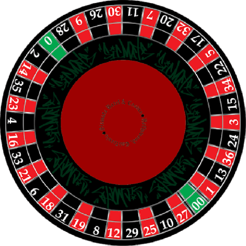
To keep the exposition concrete, consider a classic random experiment: spinning a roulette wheel.Footnote 8 An American roulette wheel has thirty-eight pockets labeled 1–36 and 0 and 00. Eighteen of the pockets are red, eighteen are black, and the 0 and 00 pockets are green (see Figure 1).
An American roulette wheel with two green pockets (0, 00). French roulette wheels have only a single green pocket.

The outcomes set comprises the possible outcomes of a spin of the wheel
 $$\begin{eqnarray}S=\{1,2,\ldots ,36,0,00\}.\end{eqnarray}$$
The 1 pocket is an elementary element in
 $S$
,
 $1\in S$
, and the outcome “landed on red” (
 $R$
) is an event, which is a subset of the outcomes set,
 $R\subset S$
.Footnote
9
The complement of
 $R$
,
 $\bar{R}$
, is the set of outcomes that are in
 $S$
, but not in
 $R$
(that is, the outcomes that are black or green).
The above definitions demonstrate that there is no difference between the notion of a set used by quantitative scholars and the definition used by QCA scholars. A set for quantitative researchers does not represent “a property or a group of properties” (Schneider and Wagemann Reference Schneider and Wagemann2012, 24); it is “a collection of objects” (Binmore Reference Binmore1982, 1). In the next sections, I show the relationship between sets and random variables and sets and probability as well as the connection between random variables, probability, and Boolean algebras.
3.2 Random variables and Boolean algebras
The world does not produce data; it produces outcomes. When we spin a roulette wheel, we might be interested in the events “landed on red” (
 $R$
), “landed on black” (
 $B$
), and “landed on green” (
 $G$
). We need to assign numbers to these events in order to talk about notions such as expectation and variation. That is the job of a random variable.
Graduate students (and professors) in political science often have difficulty answering the question “What is a random variable?” Answers range from a variable that can take multiple values to a variable that is random. A random variable in actuality is just a function, and like all functions, it is a mapping between two sets. Consider a function that maps from a set
 $A$
to a set
 $B$
,
 $f:A\rightarrow B$
. The function assigns to every element in the set
 $A$
a unique element in the set
 $B$
.
In the case of a random variable, the set of outcomes produced by the world is mapped onto the set of real numbers,
 $\mathbb{R}$
.Footnote
10
Denoted by a capital letter, a random variable is the function
 $X(.):S\rightarrow \mathbb{R}$
. We can think of a random variable as a numerical representation of a set.
Let us assume that we are interested in the event “landed on red” when we spin the roulette wheel. The outcomes set is then
 $S=\{R,B,G\}$
. We can represent the event “landed on red” as 1 and “did not land on red” as 0:

Note that
 $X(.)$
is a function; it assigns a unique value in
 $\mathbb{R}$
to every outcome in
 $S$
.
Not every function, however, is a random variable. The outcomes of our random experiment, a spin of a roulette wheel, have probabilities associated with them. We know that the probability of the event “landed on red” is the number of possible red pockets divided by the total number of pockets or 18/38. The random variable we defined above assigns the number 1 to the event “landed on red,” and we need to ensure that we can assign the probability 18/38 to the number 1. The way we do that is with a field, which is also known as an algebra.
A collection
 $\Im$
of subsets of
 $S$
is a field or algebra if it meets three conditions:
-
∙ the outcomes set
$S$
is in the collection,
$S\in \Im$
; -
∙ if an event
$A$
is in the collection,
$A\in \Im$
, then its complement,
$\bar{A}$
, must also be in it,
$\bar{A}\in \Im$
; -
∙ if two events
$A$
and
$B$
are in the collection,
$A,B\in \Im$
, then their union is also in it,
$A\cup B\in \Im$
.


The definition of a field means that
 $\Im$
is nonempty and is closed under complementation, unions, and intersections.Footnote
11
If we demand that our function preserve the field, we can have no problems assigning the correct probabilities, which are derived straight from the experiment (see Section 3.3). The function we defined above is a random variable relative to the field
 $\Im =\{S,\emptyset ,R,\bar{R}\}$
. We can easily check that this collection of subsets meets the three conditions of being an algebra. First, the outcomes set
 $S$
is in the collection. Second, for every event in the collection, its complement is also included. The complement of
 $S$
is the empty set,
 $\emptyset$
, and vice versa. The complement of
 $R$
is
 $\bar{R}$
and vice versa. Third, the union of any two events must be in the collection. The union of
 $R$
and
 $\bar{R}$
is
 $S$
. The union of
 $S$
and any other event is
 $S$
, and the same is true of
 $\emptyset$
. We therefore meet the conditions for a random variable.Footnote
12
The notion of a field is important because fields are Boolean algebras. The difference is that fields do not have to be 0–1 Boolean algebras. Consider, for example, the field described above:
 $\Im =\{S,\emptyset ,R,\bar{R}\}$
.
 $\Im$
is not a 0–1 Boolean algebra (it comprises four elements), but it is a Boolean algebra with the following translations:

In fact, a straightforward way to form a Boolean algebra is through the power set
 ${\mathcal{P}}(\cdot )$
of a set
 $S$
. Consider the set
 $S=\{R,B,G\}$
from above. The power set of
 $S$
,
 ${\mathcal{P}}(S)$
, is the set of all subsets of
 $S$
, or
 $$\begin{eqnarray}{\mathcal{P}}(S)=\{\emptyset ,(R),(B),(G),(RB),(RG),(BG),S\}.\end{eqnarray}$$
 ${\mathcal{P}}(S)$
is closed under the set-theoretic operations of union, intersection, and complementation just as fields are (see Section 3.2). Although a full proof that the power set is a Boolean algebra is beyond the scope of this paper, we can see the connection by substituting any one of the subsets of
 ${\mathcal{P}}(S)$
for
 $p$
,
 $q$
, and
 $r$
in the Boolean laws above. Consider the subset
 $(R)$
:
 $$\begin{eqnarray}\displaystyle R\cap S & = & \displaystyle R\text{ becomes }R\wedge 1=R,\quad \text{and}\nonumber\\ \displaystyle R\cup \bar{R} & = & \displaystyle S\text{ becomes }R\vee R^{\prime }=1.\nonumber\end{eqnarray}$$
It should be clear that
 ${\mathcal{P}}(S)$
properly translated is a Boolean algebra. There is a deep connection between random variables and Boolean algebras.Footnote
13
3.3 Probability and Boolean algebras
So far, we have a random variable,
 $X$
, to translate the set of outcomes,
 $S$
, and the associated algebra,
 $\Im$
, into the set of real numbers,
 $\mathbb{R}_{X}$
. We now want to assign probabilities to those numbers that are consistent with the probabilities from the roulette wheel. The first step is to define probability, just like a random variable, as a function that maps sets into numbers. In this case, the function maps from the field,
 $\Im$
, defined above, to the 0–1 interval. The function
 $\Pr (.):\Im \rightarrow [0,1]$
is a probability set function if it meets three conditions:
-
∙ the probability of the outcomes set is 1,
$\Pr (S)=1$
; -
∙ the probability of any event
$A$
in the field is greater than or equal to 0,
$\Pr (A)\geqslant 0,\text{ for }A\in \Im$
; -
∙ if
$A_{1}$
and
$A_{2}$
are mutually exclusive events in
$\Im$
, the probability of their union is the sum of their probabilities,
$\Pr (A_{1}\cup A_{2})=\Pr (A_{1})+\Pr (A_{2})$
.






The random variable assigns numbers to subsets of the outcomes set, and the probability function assigns probabilities (values in the 0–1 interval) to those same subsets. We connect these two sets of numbers using a density function,
 $f_{x}(.)$
, which assigns the probabilities from the probability function to the value of the random variable. The density function tells us the probability that the random variable,
 $X$
, takes on a particular value,
 $$\begin{eqnarray}f_{x}(x):=\Pr (X=x)\quad \text{for all }x\in \mathbb{R}_{X}.\text{}^{14}\end{eqnarray}$$
In our example, the probability of “lands on red” is equivalent to
 $\Pr (X=1)$
, which is 18/38. The probability of “does not land on red” is equivalent to
 $\Pr (X=0)$
, which is 20/38. The result is a distribution,

The probability distribution is a representation of the set of outcomes of the random experiment plus the probabilities associated with those outcomes. Instead of working with the outcomes set,
 $S$
, the algebra,
 $\Im$
, and the known probabilities, we can now work with numbers that represent the outcomes set,
 $\mathbb{R}_{X}$
, and the density function,
 $f_{x}(x)$
.Footnote
15
The important thing to keep in mind is that we are still dealing with sets.
QCA scholars have little choice but concede that random variables are based on Boolean algebras, but once the sets are mapped to the real line and become numbers, the same scholars may well claim that the “setness” disappears. That is, the numbers do not have to obey the laws of Boolean algebra although the sets upon which they are based do. It is now time to link probability to Boolean algebra. Recall that the reason for defining a random variable on a field is to ensure that probabilities are assigned that do not violate the “setness” of the outcomes.
Consider a random variable
 $X$
with density:

It is certainly true that if we sum 0 and “not 0,” we get 6, not 1. However, if we add the probability of 0 and the probability of “not 0,” we do get 1,
 $$\begin{eqnarray}\Pr (0)+\Pr (\bar{0})=0.25+0.75=1.\end{eqnarray}$$
By the same token, it must be the case that
 $p\wedge p^{\prime }=0$
. Well, the probability of 0 and “not 0” occurring together is 0. These results suggest that there is a connection between probability and Boolean algebra and, in fact, probability is defined as a function on a Boolean algebra.Footnote
16
This particular fact is fairly esoteric, but the point is that all aspects of classical statistics are based on sets.
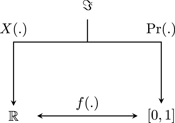
The relationship between fields, random variables, and probability. The functions
 $X(.)$
and
 $\Pr (.)$
map the real line
 $\mathbb{R}$
and the 0–1 interval, respectively, while preserving the field,
 $\Im$
. The density function
 $f(.)$
connects them.
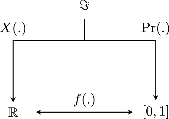
Consider Figure 2. A random variable
 $X(.)$
maps subsets of a set (a Boolean algebra) to a subset of the real line while preserving the field. Probability
 $\Pr (.)$
maps subsets of a set (a Boolean algebra) to the [0,1] interval while preserving the field. Finally, the density function
 $f(.)$
connects the random variable to the [0,1] interval. At no point in the structure depicted in Figure 2 does the “setness” of the field get lost.
3.4 Discussion
Representing sets as random variables allows us to consider operations such as addition, multiplication, or averaging. Here, the difference between QCA and statistics is starkest. When dealing with sets, QCA, which is based on the two-element Boolean algebra, allows the operations of union, intersection, and complement (see Section 2 for further explanation). However, no measure of central tendency is available; there are no means, medians, or modes. QCA users cannot discuss the notion of spread; there are no variances or ranges. There is no concept of a distribution. Few tools of any kind are available to describe or understand the state of the world.
The move to fuzzy set qualitative comparative analysis (fsQCA), which began with Ragin (Reference Ragin2000), changes nothing about these conclusions. Both traditional QCA (or crisp set QCA, csQCA) and fsQCA use the 0–1 Boolean algebra as both variants use truth tables. Ragin (Reference Ragin2008, 23) notes that “Truth tables can be built from fuzzy sets (with set membership scores ranging from 0 to 1) without dichotomizing the fuzzy scores.” The difference in the procedures lies in how one gets to the truth table. Whereas csQCA uses binary set membership (a case is either in or out of a set), fsQCA uses graduated classifications (“fully out” to “fully in”). Krogslund et al. (Reference Krogslund, Choi and Poertner2015, 23) notes that entering values into the truth table “requires reducing the findings once again to dichotomies.” Thus, fsQCA relies on the 0–1 Boolean algebra just as much as traditional QCA and is just as limited.
In contrast, the tools of quantitative methods make it easy to map from sets to averages. The key to such a mapping is that a function of random variables is a random variable. Footnote 17 Thus, everything we have previously said about random variables holds for functions of random variables, and functions of random variables are important because estimators are functions of random variables.
The sample mean
 $$\begin{eqnarray}\bar{X}=\frac{1}{n}(X_{1}+X_{2}+\cdots +X_{n}),\end{eqnarray}$$
for example, is an estimator, which is a random variable. We can derive probabilities attached to the outcomes, which would give us a density function known as a sampling distribution. Because quantitative researchers are not limited to the two-element Boolean algebra, it is possible to describe central tendency along with the attendant uncertainty. Note that the uncertainty here arises in an organic fashion directly from the uncertainty in the original experiment (the roulette wheel or a sample) and does not need to be reverse engineered (see, for example, Rohlfing (Reference Rohlfing2016) on the need for simulation in QCA). Quantitative researchers can also discuss how sets vary with one another as the linear regression estimator,
 $\hat{\boldsymbol{\unicode[STIX]{x1D6FD}}}=(\mathbf{X}^{\prime }\mathbf{X})^{-1}\mathbf{X}^{\prime }\mathbf{y}$
is, just like any other estimator, a function of random variables and therefore a random variable. None of these tools is available to QCA users. In fact, Braumoeller (Reference Braumoeller2015) and Paine (Reference Paine2016a,Reference Paineb) argue that QCA advocates must borrow the tools of conventional statistics in order to justify the conclusions that they reach.
The term “set-theoretic method” is meant to distinguish the suite of procedures associated with QCA from conventional statistical analysis. In fact, proponents of QCA and its variants use the term “set-theoretic” as a selling point. Ragin (Reference Ragin2008, 13), for example, argues that “all social science theory is verbal and, as such, is formulated in terms of sets and set relations.” In response to criticism, Ragin (Reference Ragin2005, 37) writes, “QCA is based on the algebra of sets, not on linear algebra, the basis of regression analysis. QCA’s analytic engine is fueled by set-theoretic relations, not correlations.” I have shown that conventional statistic analysis is deeply rooted in sets. The problem for qualitative researchers inclined to use QCA is that QCA has a limited menu of tools with which to manipulate and describe sets. Quantitative methods have no such restrictions.
4 Boolean algebras and logic
Any reader familiar with QCA may wonder, after learning about Boolean algebras, why QCA (the original variant or fuzzy set QCA) is limited to the two-element Boolean algebra, and the answer has to do with the connection between the two-element Boolean algebra and logic. Although researchers writing about “set-theoretic” methods often conflate the two, logic and Boolean algebra are not the same thing. Two-element Boolean algebra is a model for a kind of logic that is too weak to capture all but the simplest logical reasoning. It cannot capture temporal order (Wolfram Reference Wolfram1989), quantification (e.g., “for all” or “there exists” statements) (Genesereth and Kao Reference Genesereth and Kao2017), or other forms of generalization (Jeffrey Reference Jeffrey1991).
4.1 Preliminaries
There are many different types of logics, including propositional logic, syllogistic logic, predicate logic, modal logic, as well as nonclassical logics such as intuitionistic or constructive logic. QCA is solely concerned with propositional (also known as classical or sentential) logic, and as we shall see, only some Boolean algebras model propositional logic.
A proposition (or sentence) is a statement that is either true or false, but not both. Commands and questions are not propositions, and neither are statements such as
 $X\geqslant 5$
, because whether the statement is true depends on the value of
 $X$
. Examples of propositions include:
-
∙ David Collier studies American politics;
-
∙ the United States of America is a democracy;
-
∙ the Red Sox won the 2019 World Series.
All three statements are either true or false. Propositional logic concerns these kinds of simple sentences and their connectives (and, or, not). The sentences or propositions are denoted by symbols such as
 $P$
,
 $Q$
, and
 $S$
, and the user defines what they mean (the semantics). So I could assign the proposition “David Collier studies American politics” to the letter
 $P$
. These propositional symbols are known as atoms or atomic formulas because they contain no connectives. Thus, the proposition represented by
 $P$
is the smallest unit that the logic can analyze. Propositions in propositional logic do not have internal structure (van Benthem et al.
Reference van Benthem, van Ditmarsch, van Eijck and Jaspars2016); there are no properties. Molecules or molecular formulas are formed out of atoms and the connectives (and, or, not). If I assign the letter
 $Q$
to the proposition “The United States of America is a democracy,” then “
 $P$
and
 $Q$
” (
 $P\wedge Q$
) is a molecular formula.
A well-formed formula in propositional logic obeys the following rules:
-
∙
$P$
is a well-formed formula; -
∙ if
$P$
is a well-formed formula, then so is
$\neg P$
; -
∙ if
$P$
and
$Q$
are well-formed formulas, then so are
$P\wedge Q$
,
$P\vee Q$
,
$P\rightarrow Q$
, and
$P\leftrightarrow Q$
.


Propositional logic is truth-functional, which means that the truth of a molecular formula is a function of the truth values of the atomic propositions in it. That is, every proposition is either true or false, and every connective is truth-functional. We can therefore assess the truth value of a formula such as
 $(P\vee Q)\wedge S\rightarrow P$
by considering the truth values of the atoms
 $P$
,
 $Q$
, and
 $S$
. Truth functions are also known as Boolean functions.
The two-element Boolean algebra is a model of propositional logic because we can interpret “true” as 1, “false” as 0, and the connectives (and, or, not) as meet, join, and complement. To see the connection more completely, remember that two-element Boolean algebras have special properties. These are
 $$\begin{eqnarray}\displaystyle x\vee y=1\quad \text{if and only if }x=1\text{ or }y=1, & & \displaystyle \nonumber\\ \displaystyle x\wedge y=0\quad \text{if and only if }x=0\text{ or }y=0. & & \displaystyle \nonumber\end{eqnarray}$$
We can write these special properties in what is known as an arithmetic table for the join operator
 $\vee$
and the meet operator
 $\wedge$
:

We can compare these arithmetic tables to the truth tables for the logical “or” and “and” in propositional logic:

In the arithmetic table for
 $\vee$
, whenever a 1 appears on top or the left side, the outcome of the join operator is 1. In the truth table for “or,” whenever a T appears under
 $P$
or
 $Q$
, a T appears under
 $P\vee Q$
. The operations take on the value 0 or F only when both inputs are 0 or F. In the arithmetic table for
 $\wedge$
, only when a 1 appears on top and on the left side is the outcome 1. In the truth table for “and,” only when T appears under
 $P$
and
 $Q$
does a T appear under
 $P\wedge Q$
. The operations take on the value 1 or T only when both inputs are 1 or T. The correspondence is one to one.
A less simple Boolean algebra, such as the power set
 ${\mathcal{P}}(S)$
discussed above, is not a model of propositional logic. We can interpret
 $S$
as “true” and
 $\emptyset$
as “false,” but what of the other values in the set? QCA is inextricably tied to propositional logic because it uses two-element Boolean algebra.
4.2 The limitations of propositional logic
Propositional logic, although of immense importance to computer design (0s and 1s) and electrical engineering (on and off), has serious limitations, and contrary to the claims of QCA proponents, social theory is often too complex to be rendered in propositional logic. Consider, for example, the following perfectly sound argument (known as a syllogism):

This argument cannot be expressed in propositional logic. Recall that the smallest unit of analysis, the atom, is a true or false sentence, and we assign a unique letter to each sentence. The logic ignores the structure of the atom. That is, propositional logic cannot “see” inside the sentences (Jeffrey Reference Jeffrey1991). In the second premise, there is an object (the United States) and a property of that object (a legislature). Both, however, are hidden when we assign a letter. So we might assign
 $L$
to the first premise,
 $D$
to the second premise, and
 $U$
to the conclusion. The result,
 $L$
,
 $D$
, and therefore
 $U$
, is not valid (if the premises are true, the conclusion must be true).
 $U$
does not necessarily follow from
 $L\,,D$
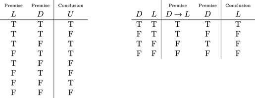
. We can see this from the left-hand truth table in Table 1, which lists all possible combinations of true and false for the three propositions.
Two propositional logics, only one of which is valid. The logic on the left is invalid because the conclusion is not necessarily true when both premises are true. The logic on the right is valid because the conclusion is true only when both premises are true.
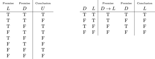
In the second line of the left-hand table, we see that both premises are true, but the conclusion is false. The takeaway is not that the natural language argument is false, but that the natural language argument cannot be proven in propositional logic.Footnote
18
The only valid rendering of the argument requires making a different argument. If the premises were, “If the United States is a democracy, then the United States has a legislature” (
 $D\rightarrow L$
) and “the United States is a democracy” (
 $D$
), we could validly conclude that “the United States has a legislature” (
 $L$
), or
 $D\rightarrow L,D\vdash L$
. The validity of this logic is demonstrated in the right-hand truth table in Table 1. The conclusions is true only when both premises are true.
We cannot use propositional logic to identity traits or properties that units may have in common such as “democracies have legislatures.” That, in turn, makes it difficult, if not impossible, to generalize or talk of patterns (Lemmon Reference Lemmon1992). The implications for QCA are dramatic. Goertz and Mahoney (Reference Goertz and Mahoney2012, 193), for example, begin their discussion of “qualitative generalizations” by pointing to statements that “All
 $A$
are
 $B$
,” and arguing that such generalizations have the form of “covering laws.” The example they give matches the democracies have legislatures example nicely,

The same problems exist, however. These statements cannot be connected using propositional logic.
The weaknesses of propositional logic led to the development of predicate logic, which introduced quantifiers (the universal
 $\forall$
and the existential
 $\exists$
), variables, and relations. Whereas propositional logic ignores the internal structure of propositions, predicate logic considers internal structure including properties and relations. A predicate is a generalization of a proposition, and predicate logic provides a “more powerful language than expressions involving only propositions” (Aho and Ullman Reference Aho and Ullman1994, 733). Using quantifiers and properties, a generalization such as “All democracies have a legislature” is easily translated as
 $\forall x(democracy(x)\rightarrow legislature(x))$
. More generally, covering law explanations of the kind Goertz and Mahoney (Reference Goertz and Mahoney2012) write about have the form (Tan Reference Tan1997, 361)

which is written in predicate logic, not propositional logic. Two-element Boolean algebra, however, is not a model for predicate logic, which requires Halmos algebra or cylindric algebra.Footnote 19
4.3 Discussion
A core claim made by QCA proponents is that qualitative scholars speak the language of logic, and that QCA captures that language. The problem with this claim is that the logic represented by the two-element Boolean algebra, propositional logic, is a weak language. Propositional logic cannot handle syllogisms (quantified logic of the form “All
 $A$
are
 $B$
”) or covering laws. Moreover, many well-established results in social science are neither syllogisms nor covering laws and still cannot be captured by QCA. The best known may be Arrow’s impossibility theorem, which relies heavily on quantifiers and cannot be written in propositional logic. At the start of his book, (Arrow Reference Arrow1963, 11) writes that the notation he uses is “familiar in mathematics and particularly in symbolic logic.” Some of the “familiar” symbols he uses are the universal quantifier and the existential quantifier, neither of which exist in propositional logic. Even the most straightforward proofs of Arrow’s theorem require quantifiers (see, for example, Geanakoplos Reference Geanakoplos2005, Fey Reference Fey2014), as do recent attempts to formalize Arrow’s theorem in logic (Wiedijk Reference Wiedijk2007; Grandi and Endriss Reference Grandi, Endriss, He, Horty and Pacuit2009; Nipkow Reference Nipkow2009). Social science is a complex endeavor, and the propositional logic embedded in QCA is too simple a language to handle it. In the next section, I show that the limitations of propositional logic restricts how QCA proponents understand causality.
5 Causation and propositional logic
QCA scholars understand causality in terms of necessity and sufficiency. Schneider and Wagemann (Reference Schneider and Wagemann2012, 53) write, “whenever set-theoretic methods are employed in order to investigate potentially causal relations between a set of conditions and an outcome set—as is done in QCA—then the aim essentially consists in unraveling necessary and sufficient conditions and combinations of these two types of causes, such as INUS and SUIN conditions.” QCA’s focus on regularity accounts of causation—what Scheines (Reference Scheines2002, 160) refers to as “causal analysis before the computer”—strikes one as odd. While most social scientists have moved on to either a counterfactual or potential outcomes conception of causality, QCA scholars remain devoted to these regularity accounts that have their roots in the 18th century. This choice becomes less inexplicable when we understand that QCA researchers equate “necessity” and “sufficiency” with the implication symbol (
 $\rightarrow$
) in propositional logic. Thus, QCA’s two-element Boolean analysis can provide the researcher with causal conditions. Counterfactual causation, however, cannot be understood through propositional logic.
Schneider and Wagemann (Reference Schneider and Wagemann2012, Chapter 3) define a sufficient condition as
 $X\rightarrow Y$
and define a necessary condition as
 $Y\leftarrow X$
. They do not actually define an INUS condition (an insufficient but necessary part of an unnecessary but sufficient condition), opting instead for an example. In their example [79],
 $A$
is an INUS condition because it is an insufficient but necessary part of the conjunction
 $(A\wedge B)$
, but the conjunction is an unnecessary but sufficient condition for
 $Y$
:
 $$\begin{eqnarray}(A\wedge B)\vee (\neg B\wedge C)\vee (D\wedge \neg F)\rightarrow Y.\end{eqnarray}$$
Kleinberg (Reference Kleinberg2010, 11) provides the necessary definition, and it can be represented in propositional logic:
 $A$
is an INUS condition of
 $Y$
if and only if for
 $A$
,
 $C$
:
 $(A\wedge B)\vee C$
is a necessary and sufficient condition of
 $Y$
, but
 $A$
is not sufficient for
 $Y$
, and
 $B$
is not sufficient for
 $Y$
.
The fact that these regularity accounts of causation can be written in propositional logic means that they can be expressed in terms of the two-element Boolean algebra.Footnote
20
More sophisticated accounts of causality, such as counterfactual accounts, cannot be written in propositional logic (see Pearl Reference Pearl2009, Chapter 7, for an extended discussion). As I noted in Section 4, propositional logic is truth-functional. That is, the truth of statements such as
 $X\rightarrow Y$
is a function of the truth of
 $X$
and
 $Y$
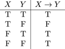
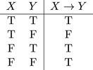
. Consider the truth table for implication (
 $\rightarrow$
) in Table 2.
 $X\rightarrow Y$
is always true when the antecedent
 $X$
is false, and
 $X\rightarrow Y$
is always true when the consequent
 $Y$
is true. Counterfactuals, however, do not work this way; they are not truth-functional. For example, consider the counterfactual, “If Collier had not attended the University of Chicago, he would have been an Americanist.” The antecedent is false (Collier went to the University of Chicago), and yet we do not want to say that the sentence is true. The conditional therefore violates the third and fourth rows of Table 2. Now consider the counterfactual, “If Collier had not finished his Ph.D., he would be a university professor.” This time the consequent is true (Collier is a university professor), but again, we do not want to say the conditional is true. This example violates the first and third rows of Table 2.
The truth table for implication (material conditional).
 $X\rightarrow Y$
takes the value false only when
 $X$
takes the value true and
 $Y$
takes the value false.
Some QCA theorists attempt to express counterfactuals in propositional logic as
 $\neg X\rightarrow \neg Y$
, the absence of
 $X$
is sufficient for the absence of
 $Y$
(Goertz and Mahoney Reference Goertz and Mahoney2012, 80). There is nothing counterfactual, or even causal, about this statement; it is simply the material conditional. We know that
 $\neg X\rightarrow \neg Y$
is not a counterfactual because it is truth-functional; that is, it corresponds to the truth table for implication in Table 2 (it is false when only the consequent is false). The antecedent of an actual counterfactual claim is false (“if
 $X$
had been otherwise”) as opposed to absent (“not
 $X$
”).Footnote
21
Rendering counterfactuals in formal logic requires a new operator,
 $X\,\Box \rightarrow Y$
, which reads “if it were the case that
 $X$
, then it would be the case that
 $Y$
” (Lewis Reference Lewis2001). The operator
 $\Box$
does not exist in propositional logic and has no counterpart in two-element Boolean algebra. (It does exist in modal logic.) Users of QCA are limited to regularity accounts of causation because these can be understood in terms of propositional logic.
5.1 Discussion
QCA users are limited to regularity accounts of causation due to QCA’s reliance on propositional logic. Users of quantitative methods face no such restrictions. While regularity accounts have well known problems (see, for example, Kim (Reference Kim1971) for a philosophical critique of INUS conditions and Brady (Reference Brady and Goodin2018) for a social science perspective), quantitative researchers may still reasonably wish to make use of the notions of necessity, sufficiency, or INUS conditions. Three possibilities for doing so exist. One option is logic regression (Ruczinski et al. Reference Ruczinski, Kooperberg and LeBlanc2003), where the predictors are Boolean combinations of binary covariates. An R package, LogicReg, exists for fitting these models. Another option is saturated regression (a model with a parameter for each unique combination of the covariates), about which Blair et al. (Reference Blair, Cooper, Coppock and Humphreys2019, 848) write “QCA via saturated regression can recover the data generating process correctly and the configuration of causes estimand can then be computed, correctly, from estimated marginal effects.” A third option is structural causal modeling (Pearl Reference Pearl2009). A key paper in this tradition is VanderWeele and Robins (Reference VanderWeele and Robins2009), in which the authors explicitly combine INUS conditions and counterfactuals within the directed acyclic graph causal framework. They do this by noting the strong similarity between Mackie’s (Reference Mackie1965) INUS conditions and Rothman’s (Reference Rothman1976) sufficient-component causes. They demonstrate how minimal sufficient conjunctions (their version of INUS or sufficient-component causes) can be represented on causal directed acyclic graphs, and then they demonstrate how minimal sufficient conjunctions relate to testable restrictions on observable data. Quantitative scholars interested in regularity accounts of causation are not limited by their methods.
6 Conclusion
QCA has seen enormous growth over the last 30 years despite strong criticism. Part of the appeal comes from proponents’ claims that QCA is based on sets and captures the natural language of social science. In operational terms, “set-theoretic” translates into 0–1 Boolean algebra, and “natural language” translates into propositional logic. What is overlooked is how restrictive these tools are when it comes to analyzing social science. First, I show that two-element Boolean algebra limits what we can say about sets and their interactions in ways that quantitative methods, which are based on more general Boolean algebras, do not. Second, I show that propositional logic is too weak a logical language to deal with simple syllogisms and covering laws, never mind contemporary social science theories. Third, I show that QCA restricts researchers to thinking about causation in terms of necessity, sufficiency, and INUS conditions, as opposed to more modern conceptions of causation such as counterfactuals. Those who wish to think about causality in terms of regularity have quantitative options for doing so. QCA occupies an unnecessary middle ground between true qualitative research and quantitative research; its putative benefits do not outweigh its limitations.
Acknowledgments
I presented earlier versions of this research at the 7th Annual Meeting of the European Political Science Association, Milan, Italy, June 2017, and the 114th APSA Annual Meeting, Boston, Massachusetts, September 2018. I thank Bear Braumoeller, John Duggan, Heather Edes, Mark Fey, Gretchen Helmke, Bethany Lacina, Jack Paine, Michael Peress, David Primo, Jason Seawright, the editor, and three anonymous reviewers for comments and suggestions. Special thanks to David Collier for many helpful discussions and suggestions. All errors are my own.
Appendix. Translating Boolean expressions
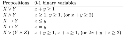
A common belief among QCA researchers is that Boolean algebra and linear algebra are, in the words of Thiem, Baumgartner, and Bol (Reference Thiem, Baumgartner and Bol2016, 748), “incommensurate.” Translating logical expressions into algebraic ones crops up in optimization problems that are subject to if-then constraints. The branch of optimization that deals with such problems is known as linear programming (LP). Integer linear programming (ILP) concerns mathematical optimization, where some or all of the variables are integers. If all of the variables are integer, it is a pure integer linear program; if some of the variables are integer, it is a mixed integer linear program (MILP). If the variables are Boolean, it is a 0–1 linear program.
Some ILP problems are formulated in Boolean propositions and predicate logic. The optimization problems that ILP can solve need not concern us. What is of interest is how logical expressions can be translated into mathematical expressions. Hürlimann (Reference Hürlimann2019, 5) writes, “Whether the problem is formulated in a purely mathematical notational framework or partially in logic is basically the same, because one can translate logical expressions into mathematical ones, and vice versa.”
The method is straightforward. First, every propositional formula can be written in the conjunctive normal form (CNF), which is a conjunction of disjunctions (van Benthem et al.
Reference van Benthem, van Ditmarsch, van Eijck and Jaspars2016). Thus, a formula of the type
 $A_{1}\wedge A_{2}\wedge \cdots \wedge A_{n}$
, where each
 $A_{i}$
is a disjunction, is in conjunctive normal form. A single disjunction (the case where
 $n=1$
), such as
 $x\vee \neg x$
(see Section 2), is already in CNF (Lemmon Reference Lemmon1992, 190). A Boolean expression is converted to conjunctive normal form using the normal tools of propositional logic (e.g., De Morgan’s laws, double negation, and the distributive laws).
Once the logical expression is in CNF, one simply transforms each clause into a linear constraint. The Boolean
 $x$
is treated as a real variable
 $x$
, and
 $\neg x$
is treated as
 $1-x$
. Any book on ILP contains a table of these transformations. Table 3 is a partial reproduction of Hürlimann’s (Reference Hürlimann2019, Table 5).
Logic-mathematical equivalences.
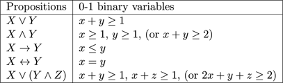
Another way to think of this problem is to define a binary variable
 $\unicode[STIX]{x1D6FF}_{j}$
that takes on only the values 0 and 1:
 $$\begin{eqnarray}\unicode[STIX]{x1D6FF}_{j}=\left\{\begin{array}{@{}ll@{}}1 & \text{if proposition }P_{j}\text{ is true},\\ 0 & \text{if proposition }P_{i}\text{ is false}.\end{array}\right.\end{eqnarray}$$
A Boolean expression as
 $(P_{1}\wedge P_{2})\rightarrow P_{3}$
is then easily translated into
 $\unicode[STIX]{x1D6FF}_{1}+\unicode[STIX]{x1D6FF}_{2}\leqslant 1+\unicode[STIX]{x1D6FF}_{3}$
.