


1 Introduction
The open cavity flow problem has been extensively investigated in the literature, aiming to predict and understand the relevant flow instabilities emanating inside cavities. This problem appears in numerous industrial applications, including open roofs on motor vehicles, landing gear in aeroplanes or dispersion of contaminants in cities. An understanding of the richness of the physics involved in this problem is therefore indispensable to designers in their endeavour to reduce noise levels, vibrations and drag in open cavity configurations.
The majority of the early work focused on the two-dimensional flow/feedback mechanism that produces self-sustained oscillations in the shear layer, commonly known as the Rossiter modes (Rossiter Reference Rossiter1964; Rockwell Reference Rockwell1977; Rockwell & Naudascher Reference Rockwell and Naudascher1979). As the incoming flow goes through the leading facing step of the cavity, recirculation vortices are developed and travel with the flow, impinging the rear face of the cavity and generating pressure waves that propagate upstream. These waves reach the leading edge of the cavity, creating a feedback mechanism that continually reinforces the shear layer oscillations, resulting in vortex shedding at the leading edge (Powell Reference Powell1953). According to Rockwell & Naudascher (Reference Rockwell and Naudascher1979), this process can be acoustic or hydrodynamic, depending on the streamwise length of the cavity. In compressible flow, Rossiter modelled an empirical formula to predict the discrete locked-on frequencies of the self-sustained modes, based on the parameters free-stream velocity and cavity length (Powell Reference Powell1961; Rossiter Reference Rossiter1964). Subsequent studies demonstrated that the feedback phenomenon is instantaneous in the incompressible regime (Mach number
 $=$
0) (Sarohia Reference Sarohia1977; Basley et al.
Reference Basley, Pastur, Lusseyran, Faure and Delprat2011; Yamouni, Sipp & Jacquin Reference Yamouni, Sipp and Jacquin2013).
Further research observed a modulation of the shear layer modes at smaller frequencies (Rockwell & Knisely Reference Rockwell and Knisely1980; Knisely & Rockwell Reference Knisely and Rockwell1982; Ziada & Rockwell Reference Ziada and Rockwell1982; Koseff & Street Reference Koseff and Street1984; Neary & Stephanoff Reference Neary and Stephanoff1987) as a result of the onset of centrifugal-type instabilities along the two-dimensional recirculating flow, which induce spanwise exchanges of fluid (Sipp & Jacquin Reference Sipp and Jacquin2000). These disturbances emerge from the combination of Görtler and Taylor–Couette instabilities (Faure et al. Reference Faure, Pastur, Lusseyran, Fraigneau and Bisch2009), generally developing inside cavities with span-to-depth ratios larger than 4 and at relatively low Reynolds numbers (Basley et al. Reference Basley, Pastur, Lusseyran, Soria and Delprat2014). While the first type of instability is developed from centrifugal forces in boundary layer flows over curved surfaces (Floryan Reference Floryan1991), the latter type of instability appears along the recirculating flow near the cavity walls, in closed-streamline flow regions where the magnitude of the angular velocity decreases towards the outward direction of the recirculation (Brès & Colonius Reference Brès and Colonius2008). This last criterion, originally provided by Rayleigh for basic inviscid swirling flows, is commonly employed in several configurations to identify parts of the flow that are centrifugally unstable (e.g. Barkley, Gomes & Henderson (Reference Barkley, Gomes and Henderson2002) in a backward-facing step, Migeon (Reference Migeon2002) in lid-driven cavities and Brès & Colonius (Reference Brès and Colonius2008) in open cavities).
The development of centrifugal instabilities inside the open cavity causes the exponential growth of three-dimensional disturbances, which reach a saturated state when the linear growth dynamics is suppressed by nonlinear effects (Schmid & Henningson Reference Schmid and Henningson2001). This allows one to define the flow as saturated when the growth of the three-dimensional structures stops being exponential. In the saturated regime, the spanwise cavity flow exhibits a row of coherent counter-rotating vortices along the span of the cavity, organized with a certain periodic pattern. These Taylor–Görtler structures pulsate and coil around the main recirculation flow inside the cavity, and present spanwise wavelengths in the order of the cavity depth (
 $\unicode[STIX]{x1D706}_{z}\sim D$
) (Faure et al.
Reference Faure, Pastur, Lusseyran, Fraigneau and Bisch2009; Basley et al.
Reference Basley, Pastur, Lusseyran, Soria and Delprat2014; Douay, Pastur & Lusseyran Reference Douay, Pastur and Lusseyran2016). The first linear computations of these three-dimensional instabilities were presented in Theofilis & Colonius (Reference Theofilis and Colonius2004), and they were proven to be dominant under certain flow conditions, as well as independent of the two-dimensional shear layer modes, from the work of Brès & Colonius (Reference Brès and Colonius2008). Their linear stability analysis results showed also that the unstable centrifugal modes oscillate with frequencies one order of magnitude lower than the 2D shear layer modes, confirming the previously observed low-frequency modulation of the shear layer oscillations. A thorough discussion on the nature of the interactions between these two types of modes was recently given by Basley et al. (Reference Basley, Pastur, Lusseyran, Soria and Delprat2014). Faure et al. (Reference Faure, Pastur, Lusseyran, Fraigneau and Bisch2009) performed an experimental campaign focusing on the visualization and characterization of these centrifugal modes inside the cavity, as functions of Reynolds number, aspect ratio and span ratio, and identified thresholds for their appearance. They also reported for the first time in open cavities a slow drift motion of the centrifugal instabilities from the centre of the cavity towards its spanwise bounding walls (Faure et al.
Reference Faure, Adrianos, Lusseyran and Pastur2007). It was postulated by the authors that this behaviour was due to the development of secondary spanwise flows in the inner part of the cavity from the sides towards the centreline, resulting from Bödewadt (Ekman-like) layers as a consequence of the presence of spanwise walls (Albensoeder, Kuhlmann & Rath Reference Albensoeder, Kuhlmann and Rath2001; Guermond et al.
Reference Guermond, Migeon, Pineau and Quartapelle2002; Migeon, Pineau & Texier Reference Migeon, Pineau and Texier2003; Albensoeder & Kuhlmann Reference Albensoeder and Kuhlmann2006). In a recent experimental parametric study of the centrifugal instabilities in an open cavity flow, Douay et al. (Reference Douay, Pastur and Lusseyran2016) observed that the reduction of the spanwise length of the cavity strengthens the sidewall effect, favouring the appearance of stationary perturbations in contrast to oscillatory ones. These results were in agreement with Faure et al. (Reference Faure, Pastur, Lusseyran, Fraigneau and Bisch2009), who tracked an increase in the drift velocity of the travelling disturbances with respect to the span ratio of the cavity.
Similar spanwise dynamics arising in the recirculating flow inside open cavities were previously observed in different flow configurations. In the flow past a backward-facing step, its centrifugal instabilities were notably treated in the work of Barkley et al. (Reference Barkley, Gomes and Henderson2002). In lid-driven cavities, cells of Taylor–Görtler vortices are also developed from centrifugal instabilities along its recirculating flow, regardless of the shear layer oscillations, as described in the works of Ramanan & Homsy (Reference Ramanan and Homsy1994), Kuhlmann, Wanschura & Rath (Reference Kuhlmann, Wanschura and Rath1997), Albensoeder et al. (Reference Albensoeder, Kuhlmann and Rath2001), Theofilis, Duck & Owen (Reference Theofilis, Duck and Owen2004), Albensoeder & Kuhlmann (Reference Albensoeder and Kuhlmann2006), de Vicente et al. (Reference de Vicente, Rodríguez, Theofilis and Valero2011) and González et al. (Reference González, Ahmed, Kühnen, Kuhlmann and Theofilis2011), among others.
For a deeper understanding of the physics involved, an extensive parametric study of the three-dimensional dynamics inside the open cavity, using linear stability analysis, was presented in Meseguer-Garrido et al. (Reference Meseguer-Garrido, de Vicente, Valero and Theofilis2014) for the incompressible limit. By investigating the behaviour of the linear eigenmodes for the significant parameters of the problem (i.e. length-to-depth aspect ratio of the cavity
 $L/D$
, Reynolds number based on the cavity depth
 $Re_{D}$
, incoming boundary layer momentum thickness
 $\unicode[STIX]{x1D703}_{0}/D$
and spanwise length of the perturbation
 $\tilde{L}_{z}$
, which can also be considered through the spanwise wavenumber,
 $\unicode[STIX]{x1D6FD}$
), the authors were able to extract the morphological structures and characteristic frequencies of the eigenmodes, and present neutral stability curves and dependence laws between the different parameters. In de Vicente et al. (Reference de Vicente, Basley, Meseguer-Garrido, Soria and Theofilis2014), the results described by linear analysis were compared with experimental results for two different set-ups in an
 $L/D=2$
cavity:
 $Re_{D}=1500$
(case A) and
 $Re_{D}=2400$
(case B). The main coherent structures present in the saturated and wall-bounded regime were found to match the ones of linear stability analysis, given the difference in flow conditions. Nonetheless, one of the main results obtained from the aforementioned experimental campaign was the apparent reduction of the characteristic frequencies of the most energetic Fourier modes from the theoretical values predicted by the linear analysis. The authors postulated that this frequency reduction was a consequence of the presence of the spanwise walls, which had the effect of slowing down the main centrifugal recirculation, thus reducing the characteristic Strouhal number of these structures. Other possible sources for this phenomenon not considered in their work could be the saturated regime of the flow or the onset of nonlinear interactions between several unstable modes.
In an attempt to further investigate the physics that led to the reduction of the characteristic Strouhal number of the most energetic mode, a three-dimensional direct numerical simulation (DNS) of the incompressible open cavity flow was employed in Vinha et al. (Reference Vinha, Meseguer-Garrido, de Vicente and Valero2016). In this study, a dynamic mode decomposition (DMD) algorithm (Schmid Reference Schmid2010) was applied from the linear to the saturated regime, with the objective of understanding the evolution of spanwise instabilities of the flow and the interactions between different dynamic modes. The case studied in Vinha et al. (Reference Vinha, Meseguer-Garrido, de Vicente and Valero2016) corresponds to the experimental case B of de Vicente et al. (Reference de Vicente, Basley, Meseguer-Garrido, Soria and Theofilis2014) (
 $Re_{D}=2400$
), as it presents a greater variety of linearly unstable modes. However, to simplify the analysis and reduce the amount of interaction between the different modes, the spanwise length of the computational domain
 $L_{z}/D$
was restricted to
 $2\unicode[STIX]{x03C0}/6$
. By doing this, the authors guaranteed that only the modes of
 $\unicode[STIX]{x1D6FD}$
that were multiples of 6, which are those corresponding to the
 $\unicode[STIX]{x1D6FD}$
of maximum amplification of the linear modes (
 $\unicode[STIX]{x1D6FD}=6$
and
 $\unicode[STIX]{x1D6FD}=12$
), appeared in the DNS solutions. The effect of the presence of spanwise walls was also neglected by imposing periodic boundary conditions on the simulations. The reduction of the characteristic Strouhal number of the dominant mode was found again after applying the DMD to snapshots within the saturated regime, contradicting the hypothesis deduced in de Vicente et al. (Reference de Vicente, Basley, Meseguer-Garrido, Soria and Theofilis2014). Nonetheless, the nature of this study and its simplifications have not proved sufficient to determine whether this effect is due to the saturated regime of the cavity flow or to secondary instabilities resulting from the occurrence of nonlinear interactions between the different unstable primary modes evolving from the base state.
This paper extends the previous research of the authors on the spanwise dynamics of saturation inside an open cavity, and presents a comprehensive numerical analysis of the entire saturation process. Direct numerical simulations of the full open cavity geometry are performed for the same inflow conditions as the abovementioned experimental case B, with a spanwise length of the computational domain
 $L_{z}/D$
in agreement with the experimental one. Thus, the forced selection of spanwise wavenumber is diminished, allowing a greater variety of modes to interact. Additionally, two distinct spanwise boundary conditions are imposed in order to determine the true nature of the reported drop in Strouhal number, namely spanwise walls bounding the computational domain, but also spanwise periodic boundary conditions to cancel the effect of the presence of walls, allowing more comprehensive comparisons. A DMD technique is applied to both cases for the identification of the relevant dynamic modes within the saturated flow. Both temporal and spatial modal analyses are performed to capture the frequency and spanwise wavenumber of the relevant perturbations.
2 Methodology
2.1 Problem description
A schematic representation of the flow configuration is depicted in figure 1. The parameters that completely define the incoming flow are (i) the Reynolds number based on the cavity depth (
 $Re_{D}=U_{\infty }D/\unicode[STIX]{x1D708}$
, where
 $U_{\infty }$
is the free-stream velocity, and
 $\unicode[STIX]{x1D708}$
is the kinematic viscosity) and (ii) the incoming boundary layer momentum thickness (
 $\unicode[STIX]{x1D703}_{0}/D$
). The geometrical parameters of the cavity are (i) the length-to-depth aspect ratio (
 $L/D$
) and (ii) the spanwise length normalized by the cavity depth (
 $L_{z}/D$
). The case studied in the present work corresponds to the experimental case B of de Vicente et al. (Reference de Vicente, Basley, Meseguer-Garrido, Soria and Theofilis2014), with
 $Re_{D}=2400$
and
 $\unicode[STIX]{x1D703}_{0}/D=0.036$
, in a cavity with geometrical parameters
 $L/D=2$
and
 $L_{z}/D\sim 10$
.
Schematic description of the three-dimensional rectangular open cavity and the parameters of the problem (
 $\unicode[STIX]{x1D6FF}_{0}$
denotes the boundary layer thickness at the leading edge of the cavity).

2.2 Linear stability and experimental analysis
The linear stability theory is concerned with the evolution of disturbances of small amplitude superimposed over a basic state (
 $\bar{\boldsymbol{q}}$
). In this case, BiGlobal instability analysis, in which the three-dimensional space comprises an inhomogeneous two-dimensional domain that is extended periodically in
 $z$
, was used to analyse the flow over an open cavity.
The linearization of the incompressible Navier–Stokes (NS) equations around
 $\bar{\boldsymbol{q}}(\tilde{x},{\tilde{y}})$
results in
 $$\begin{eqnarray}\boldsymbol{q}(\tilde{x},{\tilde{y}},\tilde{z},t)=\bar{\boldsymbol{q}}(\tilde{x},{\tilde{y}})+\unicode[STIX]{x1D716}\hat{\boldsymbol{q}}(\tilde{x},{\tilde{y}})\text{e}^{\text{i}(\unicode[STIX]{x1D6FD}\tilde{z}-\unicode[STIX]{x1D714}t)},\end{eqnarray}$$
where
 $\unicode[STIX]{x1D6FD}=2\unicode[STIX]{x03C0}/\tilde{L}_{z}$
is the spatial wavenumber of the perturbation in the
 $z$
-direction,
 $\tilde{L}_{z}$
being its corresponding dimensionless wavelength, while
 $\unicode[STIX]{x1D714}$
stands for the frequency in the temporal instability analysis framework. In this equation, it should be noted that the three spatial directions are normalized by the cavity depth, i.e.
 $(\tilde{x},{\tilde{y}},\tilde{z})=(x/D,y/D,z/D)$
. This gives rise to the following complex generalized eigenvalue problem:
 $$\begin{eqnarray}\boldsymbol{A}(\bar{\boldsymbol{q}})\hat{\boldsymbol{q}}=\unicode[STIX]{x1D714}\hat{\boldsymbol{q}},\end{eqnarray}$$
where
 $\boldsymbol{A}(\bar{\boldsymbol{q}})$
is a linear NS operator.
The associated eigenvalue problem is then solved for the determination of the complex eigenvalue,
 $$\begin{eqnarray}\unicode[STIX]{x1D714}=2\unicode[STIX]{x03C0}\frac{\mathit{St}_{D}U_{\infty }}{D}+\text{i}\unicode[STIX]{x1D70E},\end{eqnarray}$$
where
 $\unicode[STIX]{x1D70E}$
is the amplification/damping rate of the disturbance, and the Strouhal number (
 $\mathit{St}_{D}$
) represents the dimensionless frequency based on the cavity depth.
In the range of parameters close to the limit of stability, a detailed linear stability analysis was performed by Meseguer-Garrido et al. (Reference Meseguer-Garrido, de Vicente, Valero and Theofilis2014), showing the presence of three main branches of unstable eigenmodes. These branches can be seen in the neutral curves for
 $L/D=2$
depicted in figure 2(a). The mode that becomes unstable at lower Reynolds number, mode I (represented in red in figure 2), is a travelling disturbance that is more unstable in the proximity of
 $\unicode[STIX]{x1D6FD}\simeq 6$
and
 $\unicode[STIX]{x1D6FD}\simeq 12$
. Mode II (represented in blue in figure 2), the second to become unstable, is stationary at higher
 $\unicode[STIX]{x1D6FD}$
and undergoes a bifurcation at
 $\unicode[STIX]{x1D6FD}\simeq 9$
, resulting in a pair of complex conjugate eigenvalues (so it is also a travelling mode) for values of
 $\unicode[STIX]{x1D6FD}$
lower than that. The third mode to become unstable, mode III (represented by empty circles with grey outline in figure 2
a), is also a travelling disturbance with negligible relevance for the Reynolds number of the study (
 $Re_{D}=2400$
).
Neutral stability curves for the
 $L/D=2$
cavity in the
 $Re_{D}$
versus
 $\unicode[STIX]{x1D6FD}$
plane (a) (adapted from Meseguer-Garrido et al. (Reference Meseguer-Garrido, de Vicente, Valero and Theofilis2014)). The
 $\mathit{St}_{D}$
versus
 $\unicode[STIX]{x1D6FD}$
map of unstable eigenmodes from linear stability analysis, compared with the most energetic modes of the experiments of de Vicente et al. (Reference de Vicente, Basley, Meseguer-Garrido, Soria and Theofilis2014), depicted by grey areas, at
 $Re_{D}=2400$
(b).

For this flow configuration, the comparison between previous linear stability and experimental results from de Vicente et al. (Reference de Vicente, Basley, Meseguer-Garrido, Soria and Theofilis2014) can be seen in figure 2(b) for both modes I and II in the
 $\mathit{St}_{D}$
–
 $\unicode[STIX]{x1D6FD}$
plane. The red and blue symbols refer to modes I and II of the linear stability analysis while the grey areas show the natural frequencies of the spanwise structures of the real flow in the experiments. This figure shows the discrepancy in the Strouhal numbers, already discussed in § 1, between the
 $\unicode[STIX]{x1D6FD}=2\unicode[STIX]{x03C0}$
eigenmode of mode I and the low-
 $\unicode[STIX]{x1D6FD}$
branch of mode II, and the corresponding experimental Fourier modes.
The present paper intends then to delve into the possible causes of these discrepancies in Strouhal number. Throughout this paper, the results derived from our numerical simulations are confronted with previous linear stability analysis and experimental results, entirely extracted from the work of de Vicente et al. (Reference de Vicente, Basley, Meseguer-Garrido, Soria and Theofilis2014). It should be noted that these experimental results were obtained from high-resolution particle image velocimetry measurements performed in the spanwise plane
 $y/D=-0.1$
.
The interpolated multi-domain mesh of the cavity in the streamwise/normal plane (a) and the spanwise/normal plane (b).

2.3 Direct numerical simulation
The numerical solutions required to construct the data sequences of snapshots for the DMD were obtained by means of a three-dimensional unsteady DNS solver. The incompressible laminar Navier–Stokes (NS) equations constitute a system of partial differential equations which can be written in vector form as
 $$\begin{eqnarray}\displaystyle {\displaystyle \frac{\unicode[STIX]{x2202}\boldsymbol{U}}{\unicode[STIX]{x2202}t}}+\unicode[STIX]{x1D735}\boldsymbol{\cdot }\boldsymbol{F}(\boldsymbol{U})=0, & & \displaystyle\end{eqnarray}$$
where
 $\boldsymbol{U}$
represents the vector of conservative variables and
 $\boldsymbol{F}(\boldsymbol{U})$
represents the convective and diffusive 3D fluxes.
High-order spectral type methods have been extensively used in computational fluid dynamics due to their accuracy and efficiency in the simulation of fluid flows. In particular, these methods are suitable for problems where high accuracy is required, and, hence, are well suited to tracking the evolution of small flow perturbations.
In this context, the discontinuous Galerkin spectral element method (DG-SEM) (Kopriva Reference Kopriva2009) is used in this work to solve (2.4). The original domain is divided into non-overlapping hexahedral subdomains,
 $E_{k}$
, such that
 $\unicode[STIX]{x1D6FA}=\sum _{k}E_{k}$
. Inside each subdomain, a polynomial of degree
 $N$
is used to approximate the unknowns and the fluxes,
 $\boldsymbol{U},\boldsymbol{F}$
. For details on methodology, implementation and numerical validation of the spectral discontinuous tool employed, the reader is directed to Kopriva (Reference Kopriva1998), Jacobs, Kopriva & Mashayek (Reference Jacobs, Kopriva and Mashayek2005), Kopriva (Reference Kopriva2009) and Vinha et al. (Reference Vinha, Meseguer-Garrido, de Vicente and Valero2016).
The DNS code used for the present work was compiled and executed using 64 nodes in the HPC cluster Magerit, installed in the Supercomputing and Visualization Center of Madrid (CeSViMa (http://www.cesvima.upm.es/infrastructure/hpc), Universidad Politécnica de Madrid).
2.3.1 Computational set-up
In a cavity with length-to-depth aspect ratio
 $L/D=2$
, two types of spanwise boundary conditions were investigated: spanwise bounding walls and spanwise periodicity. For the periodic case, the spanwise length was set to 10 times the one chosen in Vinha et al. (Reference Vinha, Meseguer-Garrido, de Vicente and Valero2016) (i.e.
 $L_{z}/D=10\times 2\unicode[STIX]{x03C0}/6$
), while for the second configuration, this parameter was fixed to
 $L_{z}/D=10$
, reproducing the same cavity domain as in the experiments.
A multi-block structured mesh with a total of
 $416$
hexahedral subdomains was used for the DNS computations, with nine subdomains in the streamwise direction, eight in the spanwise direction and eight in the normal direction. Inside each subdomain, a polynomial of degree
 $(N_{x},N_{y},N_{z})=(12,12,12)$
was defined. The resulting three-dimensional grid generated for the DNS is shown in figure 3. It should be noted that the grid generated near the boundaries was sufficiently refined to compute the boundary layer with accuracy.
Control parameters of the simulated cavity flow, characterizing the inflow Blasius profile.

The chosen flow conditions were the same as in the linear analysis, with the exception of the Mach number (
 $M=0.2$
). The control parameters involved in the present numerical analysis are provided in table 1. A good agreement between incompressible results from linear analysis and the low-Mach case of Brès & Colonius (Reference Brès and Colonius2008) is shown in Meseguer-Garrido et al. (Reference Meseguer-Garrido, de Vicente, Valero and Theofilis2014), while compressibility effects are still negligible at this low Mach number. Blasius profiles were imposed in a weak form at the inlet and outlet sections, while non-slip boundary conditions were applied at the walls. At the far-field boundaries, constant free-stream conditions were imposed.
The two-dimensional stationary solution was extruded into the whole computational domain, and then a random noise of
 $10^{-8}$
was introduced to kickstart the linear growth of the unstable modes. Solution snapshots of the whole flow field were saved within a period between 1 and 5 non-dimensional time units. The
 $L_{\infty }$
-norm of the spanwise velocity component of the perturbed flow was also monitored as a function of non-dimensional time (
 $\unicode[STIX]{x1D70F}=tU_{\infty }/D$
) at several control points located inside the cavity in order to determine the different regimes of the spanwise flow. This information is indispensable to perform the DMD, as is discussed in the following subsection. Moreover, since the value of this velocity component is zero in the two-dimensional base flow, the whole effect corresponds to perturbation, giving greater detail about the underlying spanwise dynamics.
2.4 Dynamic mode decomposition
The DMD is a recent data-based technique that allows the extraction of spatial modal structures from a set of data snapshots of the flow field. Each identified dynamic mode is associated with a single and unique frequency, a consequence of the orthogonalization in time of the decomposition. This technique is based on the Koopman analysis of a dynamical system (Rowley et al. Reference Rowley, Mezic, Bagheri, Schlatter and Henningson2009; Mezic Reference Mezic2013), aiming to approximate the Koopman modes and eigenvalues of a linear infinite dimensional operator that describes that system, even if its dynamic behaviour is nonlinear. Contrary to other decomposition techniques, the DMD does not rank the extracted coherent structures in terms of energy content. However, their amplitudes provide a feedback about the individual contribution of a specific mode to the original dataset (Schmid Reference Schmid2013).
The advantages offered by the DMD in the postprocessing of numerical and experimental data are ease of implementation, efficient data analysis, inherent low computational cost and possibility of application to large datasets or to subdomains of a certain flow region. Some implementations of this tool for cavity problems can be found in the literature (Seena & Sung Reference Seena and Sung2011; Gómez et al. Reference Gómez, Le Clainche, Paredes, Hermanns and Theofilis2012; Ferrer, de Vicente & Valero Reference Ferrer, de Vicente and Valero2014; Vinha et al. Reference Vinha, Meseguer-Garrido, de Vicente and Valero2016). This method has also demonstrated superior performance over other traditional data-based decomposition techniques for oscillatory dominated problems (Schmid Reference Schmid2013) and for fluid flows presenting strong peaks in the spectrum (Mezic Reference Mezic2013).
Nonetheless, it is important to be aware of its current limitations. According to Bagheri (Reference Bagheri2013), there is as of yet no validation between Koopman and DMD modes for chaotic and noisy high-Reynolds-number flow data. The works of Duke, Soria & Honnery (Reference Duke, Soria and Honnery2012) and Dawson et al. (Reference Dawson, Hemati, Williams and Rowley2016) showed also that this decomposition can be sensitive to the presence of noise in the data field. For some complex problems, the effectiveness of the DMD in approximating the associated flow field still needs to be demonstrated.
Before initializing the decomposition, flow-field snapshots have to be collected with a constant sampling frequency, dictated by the Nyquist criterion. In order to avoid aliasing and possibly a diverged decomposition, the data must be sampled at least at twice the highest frequency of the dynamic modes to be extracted. A snapshot matrix can then be constructed containing
 $N$
snapshots temporally sorted and equally spaced by a constant sampling time
 $\unicode[STIX]{x0394}t$
,
 $$\begin{eqnarray}\unicode[STIX]{x1D651}_{1}^{N}=(\boldsymbol{v}_{1},\boldsymbol{v}_{2},\boldsymbol{v}_{3},\ldots ,\boldsymbol{v}_{N}).\end{eqnarray}$$
The matrix
 $\unicode[STIX]{x1D651}_{1}^{N}$
may be composed of one or all variables of the flow field. If we consider only one flow variable, the computational cost of the DMD is substantially reduced. Nevertheless, to describe the whole dynamics of the system more accurately, as many flow-field variables as possible should be included, given that the basis of the dynamic modes is common to all of them (Richecoeur et al.
Reference Richecoeur, Hakim, Renaud and Zimmer2012). In the previous work (Vinha et al.
Reference Vinha, Meseguer-Garrido, de Vicente and Valero2016) with very similar flow conditions, the authors verified that performance of the DMD with the three velocity components of the flow, rather than use of only the spanwise velocity component, did not add relevant features to the extracted dynamic modes. The results presented and discussed in the following sections were therefore obtained using only the spanwise velocity component in the decomposition.
The aim of the DMD is to extract the dynamic characteristics of the linear operator
 $\unicode[STIX]{x1D63C}$
that approximates the dynamical process between two consecutive snapshots,
 $$\begin{eqnarray}\displaystyle & \unicode[STIX]{x1D63C}(\boldsymbol{v}_{1},\boldsymbol{v}_{2},\ldots ,\boldsymbol{v}_{N-1})=(\boldsymbol{v}_{2},\boldsymbol{v}_{3},\ldots ,\boldsymbol{v}_{N}), & \displaystyle\end{eqnarray}$$
 $$\begin{eqnarray}\displaystyle & \unicode[STIX]{x1D63C}\unicode[STIX]{x1D651}_{1}^{N-1}=\unicode[STIX]{x1D651}_{2}^{N}. & \displaystyle\end{eqnarray}$$
For a sufficiently long sequence of snapshots, the original DMD initially performs a singular value decomposition (SVD) on the snapshot matrix
 $\unicode[STIX]{x1D651}_{1}^{N-1}=\unicode[STIX]{x1D650}\unicode[STIX]{x1D72E}\unicode[STIX]{x1D652}^{H}$
in order to find a matrix
 $\unicode[STIX]{x1D64E}$
that describes the dynamics of the unknown matrix
 $\unicode[STIX]{x1D63C}$
. This guarantees higher robustness in the presence of noise and other uncertainties, or in the case of rank-deficiency data. Projecting then the matrix
 $\unicode[STIX]{x1D63C}$
onto a basis spanned by the SVD modes
 $\unicode[STIX]{x1D650}$
, and after some algebraic manipulation,
 $$\begin{eqnarray}\unicode[STIX]{x1D64E}=\unicode[STIX]{x1D650}^{H}\unicode[STIX]{x1D63C}\unicode[STIX]{x1D650}=\unicode[STIX]{x1D650}^{H}\unicode[STIX]{x1D651}_{2}^{N}\unicode[STIX]{x1D652}\unicode[STIX]{x1D72E}^{-1}.\end{eqnarray}$$
The following step consists of solving the eigenvalue problem
 $\unicode[STIX]{x1D64E}\boldsymbol{y}_{i}=\unicode[STIX]{x1D707}_{i}\boldsymbol{y}_{i}$
. The dynamic modes can finally be recovered using the expression
 $$\begin{eqnarray}\unicode[STIX]{x1D753}_{i}=\unicode[STIX]{x1D650}\boldsymbol{y}_{i}.\end{eqnarray}$$
From the imaginary part (
 $\unicode[STIX]{x1D714}_{i}$
) and real part (
 $\unicode[STIX]{x1D70E}_{i}$
) of the eigenvalues of
 $\unicode[STIX]{x1D64E}$
, we retrieve the frequency information and growth rates of the dynamic modes respectively. The eigenvalues of
 $\unicode[STIX]{x1D64E}$
can be expressed in terms of physical or dynamic information by
 $$\begin{eqnarray}\unicode[STIX]{x1D706}_{i}=\frac{1}{\unicode[STIX]{x0394}t}\log \unicode[STIX]{x1D707}_{i}.\end{eqnarray}$$
In order to recover the amplitude information of the DMD modes, the matrix
 $\unicode[STIX]{x1D651}_{1}^{N-1}$
needs to be decomposed into
 $$\begin{eqnarray}\unicode[STIX]{x1D651}_{1}^{N-1}=\unicode[STIX]{x1D731}\unicode[STIX]{x1D63F}\unicode[STIX]{x1D63E},\end{eqnarray}$$
with
 $\unicode[STIX]{x1D731}=[\unicode[STIX]{x1D753}_{1},\unicode[STIX]{x1D753}_{2},\ldots ,\unicode[STIX]{x1D753}_{N-1}]$
. The matrix
 $\unicode[STIX]{x1D63E}$
is a Vandermonde matrix that contains the identified discrete frequencies
 $\unicode[STIX]{x1D707}_{i}$
, and is expressed by
 $$\begin{eqnarray}\displaystyle \unicode[STIX]{x1D63E}=\left[\begin{array}{@{}ccccc@{}}1 & \unicode[STIX]{x1D707}_{1} & \unicode[STIX]{x1D707}_{1}^{2} & \ldots & \unicode[STIX]{x1D707}_{1}^{N-2}\\ 1 & \unicode[STIX]{x1D707}_{2} & \unicode[STIX]{x1D707}_{2}^{2} & \ldots & \unicode[STIX]{x1D707}_{2}^{N-2}\\ \vdots & & & & \vdots \\ 1 & \unicode[STIX]{x1D707}_{N-1} & \unicode[STIX]{x1D707}_{N-1}^{2} & \ldots & \unicode[STIX]{x1D707}_{N-1}^{N-2}\end{array}\right]. & & \displaystyle\end{eqnarray}$$
The matrix
 $\unicode[STIX]{x1D63F}$
is the diagonal matrix containing the amplitudes of the respective modes. In order to avoid an inversion of the matrix
 $\unicode[STIX]{x1D63E}$
and an ill-conditioned operation, one has to look for the inverse of the amplitude matrix
 $\unicode[STIX]{x1D63F}$
, following the expression (Schmid Reference Schmid2013)
 $$\begin{eqnarray}\unicode[STIX]{x1D63F}^{-1}=\unicode[STIX]{x1D63E}\unicode[STIX]{x1D652}\unicode[STIX]{x1D72E}^{-1}\boldsymbol{y}_{i}.\end{eqnarray}$$
It should be noted that
 $\unicode[STIX]{x1D63F}$
is much easier to invert than
 $\unicode[STIX]{x1D63E}$
. With this approach, it is possible to recover all of the amplitudes of the dynamic modes.
Our DMD implementation was written in the Fortran programming language. For the computation of the SVD and eigenvalue problem, the subroutines dgesvd and dgeev of LAPACK were used respectively.
3 Modal analysis of the spanwise dynamics
3.1 Cavity with periodic boundary conditions
When periodic boundary conditions are imposed on the investigated open cavity flow, two instability regions for the spanwise velocity component are identified. These regimes can be seen in figure 4(a), which shows the temporal evolution of the spanwise velocity component for three control points placed inside the cavity, with different spanwise locations. The coordinates of these points are indicated above each curve in figure 4(a). As expected, the aforementioned velocity component exhibits at these control points a linear growth phase followed by a saturated regime. As is shown in figure 4(b), the exponential growth slopes at the three DNS control points match the one predicted by linear stability analysis. In the centre of the computational domain, differences between DNS and linear growth rates are within 1 %, while in regions closer to the periodic boundaries, discrepancies can reach 7 %.
The temporal evolution of the absolute value of the spanwise velocity component at three control points located inside the cavity, from the linear to the saturated regime (a). Detail of the linear zone in logarithmic scale and comparison with linear analysis (b).

The saturated regime is reached when the nonlinear dynamics overcomes the linear behaviour of the centrifugally growing disturbances. The contribution of high-order terms to the size of the perturbation starts then to become important when the slope of the most unstable linearly growing perturbation experiences a significant change of its linear value. In this context, we accept that the saturated regime starts when the change of this slope exceeds a certain threshold value
 $\unicode[STIX]{x1D6FC}$
, i.e.
 $$\begin{eqnarray}\left|\left.\begin{array}{@{}c@{}}\text{d}w/\text{d}t\end{array}\right|_{t+\text{d}t}-\left.\begin{array}{@{}c@{}}\text{d}w/\text{d}t\end{array}\right|_{t}\right|\geqslant \unicode[STIX]{x1D6FC}.\end{eqnarray}$$
The value of
 $\unicode[STIX]{x1D6FC}$
adopted in this paper is
 $\unicode[STIX]{x1D6FC}=0.1\times \left.\begin{array}{@{}c@{}}\text{d}w/\text{d}t\end{array}\right|_{t}$
.
From figure 4, it can be inferred that saturation does not occur at the same moment for the three investigated control points due to the fact that a random numerical noise was artificially imposed for the onset of spanwise perturbations. This motivates slightly different initial states at these points, resulting in variations in the size of the perturbation of one order of magnitude. At
 $P_{1}$
and
 $P_{3}$
, saturation of the leading mode occurs at around 700 time units, while at
 $P_{2}$
, saturation seems to occur earlier. After the occurrence of saturation, the spanwise velocity component experiences an oscillatory behaviour with unstable amplitude at the three control points, with
 $\mathit{St}_{D}\approx 0.020$
.
The DMD technique was applied to each of the identified regimes in order to investigate the morphology and characteristic frequencies of the relevant modes appearing in each regime. Convergence of the DMD was assumed when the residual norm of the decomposition was sufficiently low and when the eigenvalues corresponding to the most relevant dynamic modes became independent of the number of snapshots comprising the initial matrix
 $\unicode[STIX]{x1D651}_{1}^{N}$
. The DNS solution snapshots were collected with a constant sampling frequency, which was selected taking into account the temporal evolution of the spanwise instabilities. The following subsections describe the most relevant results obtained with the DMD.
3.1.1 Linear regime
A modal analysis was conducted by applying the DMD to the linear growth regime. Recovering the first solution snapshot at
 $\unicode[STIX]{x1D70F}=250$
, this technique took 40 DNS snapshots temporally spaced by a constant
 $\unicode[STIX]{x0394}\unicode[STIX]{x1D70F}=5$
. It should be noted that only the spanwise velocity component was added to the snapshot matrix for the decomposition, as previously explained in § 2.4.
The obtained DMD spectrum is compared with the BiGlobal stability analysis performed by Meseguer-Garrido et al. (Reference Meseguer-Garrido, de Vicente, Valero and Theofilis2014). In figure 5, the real and imaginary parts of the eigenmodes are plotted. The eigenvalues from linear stability analysis are coloured with respect to the wavenumber of the perturbations. We can observe that both the frequency and the growth rate of all unstable DMD modes are in agreement with linear stability analysis results. The dominant DMD modes in the decomposition, matching each branch of the most unstable BiGlobal modes (modes I and II in figure 2), were selected to evaluate the spatial wavenumbers of those modes. The DMD modes A, B and C correspond to the stationary branch of linear mode II, the DMD mode D to the low-
 $\unicode[STIX]{x1D6FD}$
branch of linear mode II and finally the DMD modes E and F to the linear mode I.
Comparison between the obtained DMD spectrum (empty rhombuses) and the linear stability analysis (filled dots, coloured as a function of the spanwise wavenumber of the linear eigenspectrum).

Isosurfaces of spanwise velocity (on the left) and spatial FFTs (on the right) of the selected unstable DMD modes in the linear regime, obtained within the time interval 250–450. Two contour levels of spanwise velocity are displayed, namely
 $-0.0015$
and
 $0.0015$
. Coordinate axes are shown in (a).

The morphology of the selected unstable DMD modes is represented on the left of figure 6 by isosurfaces of spanwise velocity. On the right, the averaged results obtained from a spatial Fourier analysis of each DMD mode are shown. The spatial fast Fourier transforms (FFTs) were performed on the spanwise velocity component over several
 $x$
positions in the
 $y/D=-0.1$
plane. The shape of the growing DMD mode A resembles the leading disturbance from linear stability analysis. The FFT demonstrates an amplitude peak for
 $\unicode[STIX]{x1D6FD}=11.6$
, this wavenumber being in accordance with the BiGlobal analysis for the leading unstable mode. The DMD mode A did not grow uniformly over the spanwise direction, as instabilities start growing first at the centre of the cavity and later towards the periodic boundaries. This lack of homogeneity over the spanwise direction can also be observed in DMD modes B and E, and was already observed in the experimental work of de Vicente et al. (Reference de Vicente, Basley, Meseguer-Garrido, Soria and Theofilis2014). As explained before, the random nature of the initial seeding means that the base upon which the exponential growth starts can be different in each part of the computational domain. In the same way, slight inequalities in the incoming flow in the experimental set-up can affect the local morphology of the flow inside the cavity.
Spatial FFT power spectral density performed on the spanwise velocity component for each DNS snapshot. The PSD is averaged for several streamwise locations in the
 $y/D=-0.1$
plane. (a) Linear regime towards transition to the saturated regime. (b) Saturated regime.

Although the DMD is supposed to separate eigenmodes by frequency, in the present case it retrieved three unstable stationary modes (DMD modes A, B and C) that represent all of the unstable linear eigenmodes of the high-
 $\unicode[STIX]{x1D6FD}$
branch of mode II (the stationary branch shown in figure 2
b). The extraction of more than one DMD mode for a certain frequency was documented for the first time in the very recent work of le Clainche & Vega (Reference le Clainche and Vega2017), when the original DMD formulation of Schmid (Reference Schmid2010) was applied.
3.1.2 Transition to the nonlinear regime
In an attempt to characterize how transition from the linear to the nonlinear regime is produced, a spatial Fourier analysis was conducted. From the beginning of the periodic DNS until
 $\unicode[STIX]{x1D70F}=1200$
, spatial FFTs were performed on the spanwise velocity component over several streamwise positions in the
 $y/D=-0.1$
plane. The results obtained are combined in figure 7, where the amplitude of peaks in the Fourier power spectral density (PSD) is plotted over the DNS time.
The linear growth phase can clearly be observed in figure 7(a). Modes with wavenumbers in the
 $\unicode[STIX]{x1D6FD}$
range 11.5–12 are the most unstable growing ones and dominate the spectrum until saturation of these modes occurs. These observations are consistent with the DMD analysis presented in § 3.1.1 for the linear regime. Just before the leading modes saturate, at approximately
 $\unicode[STIX]{x1D70F}\simeq 650$
, we can observe that the slopes of the low-
 $\unicode[STIX]{x1D6FD}$
growing modes suddenly increase. After this moment,
 $\unicode[STIX]{x1D70F}\simeq 850$
, the flow enters a completely nonlinear regime, with no apparent predominance of a certain spanwise perturbation over the others.
Figure 7(b) concentrates the FFT data for the saturated regime, allowing us to track in time the evolution of the amplitude of the PSD of a certain mode. In the first periods right after saturation, modes with wavenumbers around
 $\unicode[STIX]{x1D6FD}\simeq 9$
are clearly dominating the spectrum. Nonetheless, the figure displays also an increase of the energy of space scales with wavenumbers in the proximity of
 $\unicode[STIX]{x1D6FD}\simeq 2\unicode[STIX]{x03C0}$
, suggesting that these structures turn dominant after a short amount of time. The strong PSD amplitude oscillations in figure 7(b) are related to the highly complex spanwise behaviour of the flow and to nonlinear interactions occurring between the different modes.
3.1.3 Saturated regime
After an initial linear growth phase, saturation of the leading mode occurs, and perturbations start to fluctuate with a characteristic Strouhal number, as previously shown in figure 4. This can also be seen in figure 8, showing for a longer DNS time the evolution of the spanwise velocity component at eight probes. These new control points are distributed over the two central subdomains of the cavity, sharing the same axial and normal coordinates but having different spanwise positions. Their coordinates are shown on the top of each graph in figure 8. The close spanwise proximity between these points allows us to capture with higher confidence the nature and characteristics of the dominant perturbations occurring in a central region of the cavity. This also influences the sampling rate at which flow-field snapshots are taken from the DNS to perform the dynamic decomposition. All of the aforementioned control points track a pulsating behaviour for the entire recorded time just after saturation, with a dominant frequency in the range
 $\mathit{St}_{D}\in (0.017,0.020)$
. These values are within the Strouhal number range of the most predominant dynamics revealed by previous experiments, and represented in figure 2 by the middle grey area. This behaviour was not recovered by linear stability analysis.
The saturated regime inside the open cavity. The temporal evolution of the absolute value of the spanwise velocity component at eight probes in the middle of the cavity
 $(0.5L,-0.5D,z)$
with different spanwise locations.

Space–time diagrams of the spanwise velocity component, extracted at
 $y/D=-0.1$
and
 $x/D=0.5$
, for the DNS time intervals (a) 1200–1700 and (b) 3000–3500, with periodic boundary conditions. Lines (1) and (3) indicate left-travelling waves while lines (2) and (4) indicate right-travelling waves.

In a first attempt to clarify the space–time dynamics of the saturated flow, figure 9 shows space–time diagrams over the spanwise direction in the planes
 $y/D=-0.1$
and
 $x/D=0.5$
for two different DNS segments,
 $1200\leqslant \unicode[STIX]{x1D70F}\leqslant 1700$
in (a) and
 $3000\leqslant \unicode[STIX]{x1D70F}\leqslant 3500$
in (b),
 $\unicode[STIX]{x1D70F}$
being the DNS dimensionless time. Contours of spanwise velocity component are shown in this figure. In the saturated regime, the flow is characterized by the presence of highly coherent left- and right-travelling waves. The phase velocity of these structures over the spanwise direction can be estimated from slopes in the space–time diagram (
 $\unicode[STIX]{x0394}m$
), as depicted in figure 9 by the lines (1), (2), (3) and (4), and it can provide a rough indication about the Strouhal number of these perturbations through the expression (Basley Reference Basley2012)
 $$\begin{eqnarray}St_{D}=\frac{w_{\unicode[STIX]{x1D711}}}{U_{\infty }}{\displaystyle \frac{\unicode[STIX]{x1D6FD}}{2\unicode[STIX]{x03C0}}}=\unicode[STIX]{x0394}m{\displaystyle \frac{\unicode[STIX]{x1D6FD}}{2\unicode[STIX]{x03C0}}},\end{eqnarray}$$
where
 $w_{\unicode[STIX]{x1D711}}$
denotes the spanwise phase velocity of the travelling waves. For the dominant wavenumber of the experiments,
 $\unicode[STIX]{x1D6FD}\simeq 6$
and
 $St_{D}\approx |\unicode[STIX]{x0394}m|$
. The absolute values of the slopes drawn in figure 9 are as follows:
 $\unicode[STIX]{x0394}m_{1}=0.019$
,
 $\unicode[STIX]{x0394}m_{2}=0.022$
,
 $\unicode[STIX]{x0394}m_{3}=0.018$
and
 $\unicode[STIX]{x0394}m_{4}=0.017$
. These values are in agreement with the experimental results described in part II of Basley (Reference Basley2012), and suggest that the leading spanwise dynamics inside the cavity remains practically unchanged after the occurrence of saturation.
The DMD was applied to the saturated regime, starting the decomposition at
 $\unicode[STIX]{x1D70F}=1222$
. The results discussed in the present subsection were obtained using 272 DNS snapshots, temporally spaced from one another by 1 non-dimensional time units (i.e. approximately 5 oscillation periods were covered), which was found to be enough for a converged decomposition. In the
 $St_{D}\in (0,0.030)$
range, the DMD technique captured nine modes, associated with nine eigenvalues of
 $\unicode[STIX]{x1D64E}$
with slightly negative real parts. These modes are plotted in the
 $\unicode[STIX]{x1D6FD}$
–
 $\mathit{St}_{D}$
plane of figure 10(a), where only a single frequency corresponds to each DMD mode, represented in this graph by a set of horizontal blue diamonds. In the
 $y/D=-0.1$
plane of each mode, spatial FFTs were performed on the spanwise velocity component over various
 $x$
positions. In figure 10(a), the size of the blue diamonds is proportional to the amplitude of the averaged PSD in the abovementioned plane. The DMD spectrum is also compared in this figure with previous linear stability analysis (BiGlobal) and experimental results.
The DMD performed for the present regime was able to capture the experimental modes, represented in figure 10(a) by the grey regions. For each DMD mode, the spanwise FFTs do not exhibit a dominant wavenumber, but instead a range of prevailing wavenumbers, as shown in the experiments. For a comprehensive comparison, four DMD modes with closer frequency to the experimental modes described in de Vicente et al. (Reference de Vicente, Basley, Meseguer-Garrido, Soria and Theofilis2014) were selected, in order of increasing frequency, namely stationary DMD mode A, DMD mode B with
 $\mathit{St}_{D}=0.0059$
, DMD mode C with
 $\mathit{St}_{D}=0.018$
and DMD mode D with
 $\mathit{St}_{D}=0.025$
. Figure 10(b) displays the isosurfaces of spanwise velocity for these modes in the
 $zy$
and
 $zx$
planes.
Extracted DMD modes for the saturated regime, starting the decomposition at
 $\unicode[STIX]{x1D70F}=1222$
and using 272 DNS snapshots. (a) Extracted DMD modes in the
 $\unicode[STIX]{x1D6FD}$
–
 $\mathit{St}_{D}$
plane. Each mode is associated with a single frequency, represented by a set of horizontal blue diamonds. The size of the diamonds is proportional to the amplitude of the PSD performed on the spanwise velocity component of each DMD mode. The DMD results are compared with data from BiGlobal (red dots) and experiments (grey areas) of de Vicente et al. (Reference de Vicente, Basley, Meseguer-Garrido, Soria and Theofilis2014). (b) Isosurfaces of spanwise velocity of the aforementioned DMD modes in the
 $zy$
and
 $zx$
planes.

The DMD mode A contains several coherent structures with similar morphological shapes along the entire spanwise direction, but with different wavenumbers. The spanwise FFTs in the
 $y/D=-0.1$
plane returned amplitude peaks within the range of
 $\unicode[STIX]{x1D6FD}\in (9,12)$
, these structures resembling the stationary branch of linear bifurcated mode II. This mode comprises also low-
 $\unicode[STIX]{x1D6FD}$
structures, as indicated by the FFTs and isosurfaces of spanwise velocity, fitting the corresponding experimental shading. It should be noted that the distribution of all of these stationary structures inside the cavity is not homogeneous.
Low-
 $\unicode[STIX]{x1D6FD}$
perturbations can also be found in DMD mode B, with higher-energy structures in the range
 $\unicode[STIX]{x1D6FD}\in (4.8,7)$
. Along the spanwise direction, these structures can mainly be found in two portions of the cavity, namely
 $2.5\leqslant z/D\leqslant 4.5$
and
 $7.5\leqslant z/D\leqslant 10$
. Even if these characteristic wavenumbers are slightly lower than the ones predicted by linear stability analysis, but within the range of the experiments, the associated structures seem to correspond to the oscillatory branch of linear mode II. Moreover, the increase of Strouhal number with the decrease of associated spatial wavenumber can also be observed with the DMD.
The DMD mode C is in the Strouhal range of the most energetic mode of the experiments, oscillating with
 $\mathit{St}_{D}=0.018$
. Coherent low-
 $\unicode[STIX]{x1D6FD}$
structures can be recognized in figure 10(b) for this mode, being in agreement with the PSD amplitude peaks shown above in the range
 $\unicode[STIX]{x1D6FD}\in (4.8,6.6)$
. They can be favourably compared with the low-
 $\unicode[STIX]{x1D6FD}$
structures of travelling linear mode I; however, with lower frequency but in accordance with the experiments. Similarly to what happens with the other discussed DMD modes within the saturated regime, and also in agreement with the experiments, these structures lose their periodicity and homogeneity inside the cavity over the spanwise direction.
Finally, DMD mode D is characterized by the presence of some coherent high-
 $\unicode[STIX]{x1D6FD}$
structures, confined to small spanwise subregions of the cavity (see
 $1.5\leqslant z/D\leqslant 5$
and
 $7.5\leqslant z/D\leqslant 10$
). The highest FFT peak occurs for
 $\unicode[STIX]{x1D6FD}=10.3$
; nonetheless, other relevant structures involving wavenumbers in the range
 $\unicode[STIX]{x1D6FD}\in (3,12)$
are also obtained for this mode. Despite its highly dynamic complexity, this highly inhomogeneous mode exhibits properties that bear strong similarity to various eigenmodes of linear mode I.
Similar DMD analyses were also carried out utilizing later time windows within the saturated regime in the decomposition, and their results resembled the dynamics already described in the present subsection and did not add new relevant information. Despite the highly nonlinear and complex nature of the saturated flow inside the cavity, the DMD technique was able to identify the most relevant modes of the linear stability analysis and the experiments. The reported drop in
 $\mathit{St}_{D}$
was also revealed in the absence of spanwise walls, strongly suggesting that this effect is directly associated with the saturation process.
3.2 Cavity with spanwise wall boundary conditions
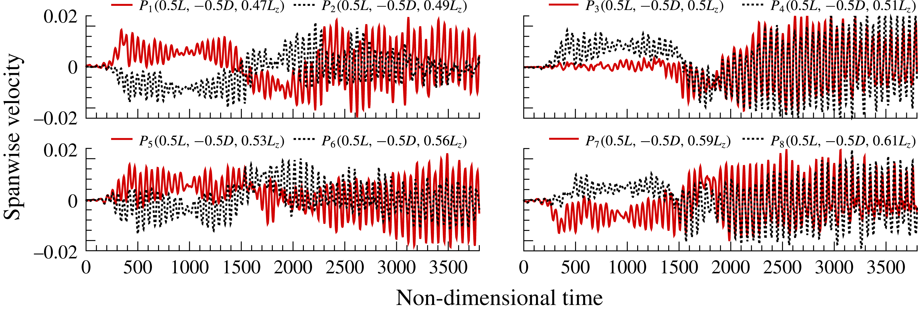
Similar investigation considering the effect of spanwise walls was also carried out. New computations were performed imposing solid wall boundary conditions at the spanwise limits of the computational domain, for the same inlet flow conditions as the periodic case. The evolution of the spanwise velocity component was tracked at eight control points distributed over the two central subdomains of the cavity. Figure 11 shows the temporal evolution of spanwise velocity at these probes, from the beginning of the DNS. The coordinates of these control points are shown at the top of their corresponding plots. Contrary to what happened in the periodic study, a linear growth regime could not be recognized for the present case. The numerical perturbation generated by the growth of the boundary layer due to the presence of lateral walls overcomes the artificial noise introduced to kickstart the DNS, triggering a faster growth of the linearly unstable modes.
The temporal evolution of the absolute value of the spanwise velocity component at eight probes in the middle of the cavity with spanwise walls.
Space–time diagram of the spanwise velocity component extracted at
 $y/D=-0.1$
and
 $x/D=0.5$
for the DNS time interval 500–3000 with spanwise bounding walls. Lines (5) and (7) indicate left-travelling waves while lines (6) and (8) indicate right-travelling waves.

From the beginning of the DNS, all control points show a wavering growth phase before spanwise velocity perturbations reach a saturated state at approximately
 $\unicode[STIX]{x1D70F}=420$
. From this moment, the spanwise velocity component fluctuates with a dominant frequency within the range
 $\mathit{St}_{D}\in (0.017,0.018)$
, inside the
 $\mathit{St}_{D}$
range of the most predominant dynamics revealed by the experiments (middle grey zone in figure 2
b), and it is related to low-
 $\unicode[STIX]{x1D6FD}$
travelling modes. These oscillations seem to reach a more stable regime around
 $\unicode[STIX]{x1D70F}=2000$
for the majority of the control points. Nonetheless, their dominant frequency remains more or less unchanged from the saturation point until the end of the computation.
As in § 3.1.3, a space–time diagram was constructed to track the temporal evolution of spanwise velocity perturbations in the saturated regime with the presence of walls in the spanwise confinements of the cavity. Once again, this variable was extracted at the
 $y/D=-0.1$
and
 $x/D=0.5$
planes for the DNS window
 $500\leqslant \unicode[STIX]{x1D70F}\leqslant 3000$
. These values were selected in order to allow a comprehensive coverage of the two main regions of velocity fluctuation previously displayed in figure 11. This diagram is shown in figure 12 in the form of spanwise velocity contours.
Due to the presence of solid walls at
 $z/D=0$
and
 $z/D=10$
, a thick horizontal band appears next to these two boundaries, delimiting a region where no periodic or stationary structures stand out and implying the formation of Bödewadt layers of opposite sign near the two end walls. The main differences between the left and right sides of figure 12 occur in the central region of the cavity, for
 $3.5\leqslant z/D\leqslant 6.5$
. On the left side, we can observe some horizontal stripes within this central region, revealing the existence of stationary perturbations. Left- and right-travelling waves also coexist in the centre of the cavity, as is suggested by the slopes (5) and (6) drawn in this figure, with absolute values
 $\unicode[STIX]{x0394}m_{5}=0.021$
and
 $\unicode[STIX]{x0394}m_{6}=0.017$
respectively. As explained in the previous section, the phase velocity of the travelling waves can be deduced from these values.
Later in the simulation, the central stationary oscillations tend to vanish as a result of saturation and onset of nonlinear interactions between the coexisting structures. This behaviour is evidenced in figure 7. At the beginning of the nonlinear regime, it can be observed that the
 $\unicode[STIX]{x1D6FD}$
modes 5 and 6 are growing at the expense of their multiples, (modes) 10 and 12 respectively, strongly suggesting that these latter modes give energy to the former ones. In the same way, modes 5 and 10 interact with modes 6 and 12, fomenting the growth of modes with wavenumbers 15 and 18 (not shown in figure 7). Eventually, when the energy of the
 $\unicode[STIX]{x1D6FD}$
modes 5 and 6 is high enough and of the same order of magnitude as the energy of the modes 10 and 12, numerous nonlinear interactions start to occur inside the cavity, giving rise to much more complex interactions between modes (see figure 7
b). Similar nonlinear behaviour is also observed in the previous work of Vinha et al. (Reference Vinha, Meseguer-Garrido, de Vicente and Valero2016). On the right side of the space–time diagram of figure 12, left- and right-travelling waves clearly dominate the spectrum inside the cavity. The absolute values of the slopes drawn on the right side of this figure are
 $\unicode[STIX]{x0394}m_{7}=0.018$
and
 $\unicode[STIX]{x0394}m_{8}=0.019$
. For the dominant wavenumber of the experiments (
 $\unicode[STIX]{x1D6FD}\simeq 6$
), these two slopes approximate the characteristic Strouhal numbers of the left and right waves (as previously shown by (3.2)).
Two different DNS time frames were selected to perform the DMD analysis. The first one started at
 $\unicode[STIX]{x1D70F}=417$
and comprised 228 snapshots while the second time interval started at
 $\unicode[STIX]{x1D70F}=1985$
and contained 291 snapshots. In both cases, the snapshots were equally spaced by a constant
 $\unicode[STIX]{x0394}\unicode[STIX]{x1D70F}=1$
. These values were chosen after performing a DMD convergence study for the two cases. Furthermore, the spatial domain of the decompositions was reduced to the six central subdomains of the mesh (
 $1.25\leqslant z/D\leqslant 8.75$
) in order to avoid the perturbations introduced by the presence of walls into the DMD.
Figure 13 summarizes the most important results obtained by means of the two DMDs. The plots on the left side were constructed for the DMD started at
 $\unicode[STIX]{x1D70F}=417$
while the ones on the right side for the DMD initiated at
 $\unicode[STIX]{x1D70F}=1985$
. The modes extracted inside the
 $St_{D}\in (0,0.030)$
range are plotted in the
 $\unicode[STIX]{x1D6FD}$
–
 $\mathit{St}_{D}$
planes of figure 13(a), where the frequency of each mode is represented by a set of horizontal diamonds. It should be noted that the corresponding eigenvalues of all of these modes have a stable behaviour. The size of the plotted diamonds is once again proportional to the amplitude of the spatial Fourier averaged PSD, performed for both cases on the spanwise velocity component over various streamwise positions in the plane
 $y/D=-0.1$
. The DMD spectrum is again confronted with data from previous linear stability analysis and experimental measurements.
Extracted DMD modes for DNS solutions with spanwise wall boundary conditions. On the left, the decomposition was started at
 $\unicode[STIX]{x1D70F}=417$
using 228 snapshots. On the right, the decomposition was started at
 $\unicode[STIX]{x1D70F}=1985$
using 291 snapshots. The spatial domain of both DMDs was reduced to the six central subdomains of the mesh. (a) Extracted DMD modes in the
 $\unicode[STIX]{x1D6FD}$
–
 $\mathit{St}_{D}$
plane. Each mode is associated with a single frequency, represented by a set of horizontal blue diamonds. The size of the diamonds is proportional to the amplitude of the PSD performed on the spanwise velocity component of each DMD mode. The DMD spectrum is compared with data from BiGlobal analysis (red dots) and experimental measurements (grey areas) of de Vicente et al. (Reference de Vicente, Basley, Meseguer-Garrido, Soria and Theofilis2014). (b) Isosurfaces of spanwise velocity of the aforementioned DMD modes in the
 $zy$
and
 $zx$
planes.

For the investigated wall-bounded cavity, both DMDs were capable of capturing modes inside the three grey areas of the experiments, with a sharp abundance of wavenumbers inside them. For a deeper comparison between the experimental Fourier and BiGlobal modes, and the extracted DMD modes, four DMD modes with closer frequency to the experimental ones were chosen. These modes are labelled by circled letters A–D in figure 13(a), in the order of increasing
 $\mathit{St}_{D}$
. Figure 13(b) shows the morphology of the DMD modes associated with those four letters, by means of isosurfaces of the spanwise velocity component (blue A–D on the left for DMD started at
 $\unicode[STIX]{x1D70F}=417$
; black A–D on the right for DMD started at
 $\unicode[STIX]{x1D70F}=1985$
).
On the left side of figure 13(b), blue DMD mode A exhibits the most coherent structures in the centre of the cavity, with wavenumbers of the order of
 $\unicode[STIX]{x1D6FD}\simeq 11$
. It should be noted that this value is close to the wavenumber for maximum amplification according to linear stability analysis (
 $\unicode[STIX]{x1D6FD}\simeq 12$
), and in agreement with the experiments. We can also notice that structures of this same mode lose some coherence in the vicinity of the walls due to the numerical establishment of the boundary layer. The existence of stationary structures mainly in the centre of the cavity was also observed on the left side of the space–time diagram of figure 12.
The black DMD mode A on the right side of figure 13(b), belonging to the second DMD time interval considered for the present analysis, shows a different morphology compared with the blue DMD mode A. We can visualize now some well-defined structures within the spanwise range
 $3\leqslant z/D\leqslant 5$
, with wavenumbers around
 $\unicode[STIX]{x1D6FD}\simeq 9$
, which is the bifurcation point from the stationary to the oscillatory branch of linear mode II. Some other structures can be seen more to the right side of the cavity (
 $6\leqslant z/D\leqslant 8$
), indicating that the distribution of structures of this stationary mode is no longer uniform inside the cavity, but inhomogeneous as in the experiments.
The left and right DMD modes B exhibit low-
 $\unicode[STIX]{x1D6FD}$
structures with wavenumbers that match the experimental grey area of figure 13(a), and they are confined to several portions of the cavity, as suggested by the isosurfaces of spanwise velocity. Other structures with smaller wavenumbers also emerge inside the cavity, possibly as a result of the growth of the boundary layer in the spanwise boundaries. Nonetheless, for the corresponding perturbation frequencies (left DMD mode B,
 $St_{D}=0.0055$
; right DMD mode B,
 $St_{D}=0.0048$
), the experiments also exhibited highly non-uniform structures with a pronounced range of wavelengths in the spanwise direction.
A similar situation occurs with the two DMD modes D displayed in figure 13(b), which are also characterized by a strong plurality of wavenumbers. The blue DMD mode D on the left is pulsating with
 $St_{D}=0.0248$
while the black DMD mode on the right with
 $St_{D}=0.0224$
. The isosurfaces of spanwise velocity display several highly inhomogeneous structures with certain coherence near the region of the walls, resembling some of the dynamics of the matching experimental mode. However, these features are not relevant in terms of energy in comparison with the ones composing the other DMD modes distinguished in figure 13 and probably evolve from nonlinear interactions between the different structures.
The most relevant mode revealed by both decompositions is DMD mode C. The blue DMD mode on the left oscillates with a characteristic
 $\mathit{St}_{D}=0.0185$
while the black one on the right with
 $\mathit{St}_{D}=0.0174$
. Both DMD modes contain clearly defined features uniformly distributed along the majority of the spanwise length of the cavity, with wavenumbers of the order of
 $\unicode[STIX]{x1D6FD}\approx 2\unicode[STIX]{x03C0}$
. On the left side, the FFT amplitude peak occurs for
 $\unicode[STIX]{x1D6FD}\simeq 5$
, while the structures on the right side present a dominant wavenumber of
 $\unicode[STIX]{x1D6FD}\simeq 6$
. In both cases, these dominant structures consist of highly coherent right- or left-travelling waves, previously observed in the space–time diagram of figure 12. The morphological shape of the present DMD modes bears thus strong similarity to the most energetic one described by the experiments, with identical shift in frequency in comparison with the linear mode I. It should be noted that a similar mode was also recovered in § 3.1.3 considering periodic boundary conditions, disclosing that the abovementioned discrepancy in frequency is not an exclusive effect of the presence of spanwise walls.
The two DMD analyses of figure 13 recovered the dominant modes of the experiments; however, a small discrepancy in frequency can be observed between the blue DMD mode C (on the left side) and the black DMD mode C (on the right side). Figure 14 compares the streamwise velocity profiles in the
 $y/D=-0.1$
plane, averaged for the following two temporal scenarios: the solid blue line uses the same DNS snapshots as in the left DMD of figure 13 while the dashed black line takes the same DNS solutions as in the right DMD of the same figure. It can be seen that the streamwise velocity in the region of the main recirculation is lower for the second case, suggesting that the saturation process has the effect of slowing down the main vortex inside the cavity, causing the aforementioned drop in
 $St_{D}$
.
Averaged dimensionless streamwise velocity profiles in the
 $y/D=-0.1$
plane considering the same DNS snapshots as in the DMDs of figure 13.

4 Discussion
With and without the presence of solid bounding walls inside the open cavity, the DMD technique was able to recover high-energy modes from a highly nonlinear and saturated flow regime, containing features that resemble the dominant structures obtained in the experimental campaign of de Vicente et al. (Reference de Vicente, Basley, Meseguer-Garrido, Soria and Theofilis2014). The frequency of those DMD modes also matched the
 $St_{D}$
range of the experiments, and confirmed the shift in frequency from the corresponding oscillatory BiGlobal mode I.
Averaged dimensionless streamwise velocity profiles within the saturated regime in the
 $y/D=-0.1$
plane. The DNS profiles are compared with the BiGlobal and experimental ones, obtained from the 2D base flow and 3D mean flow respectively and previously published in the work of de Vicente et al. (Reference de Vicente, Basley, Meseguer-Garrido, Soria and Theofilis2014) (a). Circulation around the primary vortex of the cavity, calculated out of the 3D mean flow (for the two DNS cases) and 2D base flow (linear stability analysis) (b).

Figure 15(a) shows averaged dimensionless streamwise velocity profiles for the two DNS cases studied in the present paper. These profiles were taken in the
 $y/D=-0.1$
plane and are compared with the two-dimensional base flow (i.e. a steady Navier–Stokes solution) from linear stability analysis and with the experimental mean flow averaged in time and in the spanwise direction. Within the saturated regime, we observe for both DNS cases a strong reduction of the velocity of the main recirculation, which explains the said drop in Strouhal number. This effect is consistent with previous observations of Brès & Colonius (Reference Brès and Colonius2008), which ascertained that the oscillation frequency of the three-dimensional modes is affected by the time these perturbations require to advect around the primary vortex. A reduction in the velocity of the main recirculation inside the cavity implies a longer travelling time along it, thereby contributing to a decrease in the characteristic Strouhal number of the leading centrifugal disturbance.
The trend of the maximum value of the averaged dimensionless streamwise velocity (blue squares) and circulation around the main vortex core (green diamonds) in several DNS time intervals compared with the dominant Strouhal number (red circles) retrieved by the DMD for the same time intervals: (a) DNS with spanwise periodic boundary conditions; (b) DNS with spanwise wall boundary conditions.

The circulation around the primary vortex can provide a more precise quantification of its strength. This quantity was thus estimated for the BiGlobal and DNS cases compared in figure 15(a), and it is presented in figure 15(b) normalized by its value calculated out of the base flow of the linear stability analysis. As expected, the recirculation is reduced from its two-dimensional base flow value due to the saturated regime of the three-dimensional flow for the two DNS cases. These results confirm also the strong relationship existing between the velocity of the main recirculation, or strength of this rotating region, and the oscillation frequency of the centrifugal perturbations.
A secondary effect arises from the presence of spanwise walls, leading to an additional decrease in the velocity and circulation of the main recirculation region. The development of Bödewadt layers near the spanwise end walls of the cavity motivates this further deceleration. The presence of end-wall corner vortices slowing down the main centrifugal recirculation inside the cavity was first described in the literature by Shankar & Deshpande (Reference Shankar and Deshpande2000). By comparing streamwise velocity profiles in lid-driven cavity flows, the authors observed an increasing discrepancy between the 2D (at the midplane) and 3D profiles with respect to the Reynolds number in the region of the main recirculation, with a smaller peak for the case of the 3D curves. This braking phenomenon was also observed in the experiments. Nonetheless, this effect is not as strong as the one measured inside the experimental cavity. Such discrepancies can be explained by the development of end-wall effects from the inlet of the experimental test section, yielding to more developed lateral boundary layers at the leading edge of the experimental cavity. Nevertheless, the results of figure 15 point out that the main mechanism for the reduction of frequency is the reduction of the velocity and circulation of the main vortex, and that such reduction occurs mainly due to the saturation process, while the presence of the walls is a second-order effect.
In order to attest this relationship between the recirculation velocity/strength of the main recirculation and the associated Strouhal number of the leading perturbation, the behaviour of the peak velocity of the main vortex with time, and of the frequency of the dominant DMD mode is plotted in figure 16 for both investigated DNS cases. The circulation out of the mean numerical flow is also shown in this figure, normalized by its value from the two-dimensional base flow solution. The symbols representing the parameters velocity and circulation were averaged in different DNS time intervals, and the DMDs were performed for the corresponding interval. For the periodic case (figure 16 a), the clear trend is that the saturation process reduces the recirculation velocity inside the cavity, and the frequency of the modes is reduced in the same fashion. After an initial reduction for all parameters depicted in this figure, we can observe later in the simulation a slight increase of the streamwise velocity and circulation, possibly induced by nonlinear interactions occurring inside the cavity, resulting in a small increment of the Strouhal number. However, for a much longer DNS duration, the streamwise velocity and circulation values do not change, and for this reason the oscillation frequency of the leading centrifugal mode does not vary.
For the case where lateral wall boundary conditions were imposed, figure 16(b) shows an initial trend in line with the periodic case, confirming that the reduction of Strouhal number of the leading mode is a consequence mainly of the saturation mechanism. The presence of high-energy centrifugal modes inside the cavity acts as a brake on the main recirculation, which in turn leads to a further drop in the oscillation frequency of these structures. Nonetheless, the effect of the presence of end walls also contributes to a further decrease in the velocity of the main recirculation, resulting in a stronger drop of the Strouhal number. As expected, the circulation around the primary vortex also follows this reduction trend with DNS time.
5 Concluding remarks
This paper demonstrated the capability of the DMD to analyse the spanwise perturbations occurring in an open cavity flow problem within the completely saturated regime. This technique was applied to a set of snapshots obtained from DNS, imposing lateral periodic and solid wall boundary conditions, in order to investigate the possible cause of the drop of the characteristic Strouhal number of the most energetic mode of the experiments of de Vicente et al. (Reference de Vicente, Basley, Meseguer-Garrido, Soria and Theofilis2014). Despite the highly nonlinear regime inside the cavity triggered by saturation of linearly unstable modes, the DMD was able to retrieve the morphological shapes and oscillation frequencies of the most relevant modes of the linear stability analysis and the experiments. Furthermore, similar reduction of Strouhal number was again found in the present analysis for the dominant dynamic mode, with or without the presence of spanwise bounding end walls. We found that this behaviour is mainly due to the saturated regime of the flow, which has the effect of slowing down the main centrifugal recirculation, thus reducing the characteristic Strouhal number of the modes. The presence of end-wall vortices near the spanwise confinements of the cavity only strengthens this effect, and its overall weight is always lower in comparison with saturation.
The DMD technique was revealed to be a powerful instrument in the analysis of this particular open cavity flow problem. Moreover, with the reconstruction of the dynamic modes, the DMD was demonstrated also to be a very useful tool for the visualization of the characteristics of such a complex flow field. Using this postprocessing tool, we were able to establish the link that was missing between previous experimental and linear stability analysis results, and the present DNS data, and find the true nature of the decrease in Strouhal number.
Acknowledgements
The authors would like to thank E. Ferrer for the many fruitful discussions regarding the DMD, and the European Commission for the funding received within the FP7-PEOPLE-ITN project AIRUP (Airbus–UPM European Industrial Doctorate in mathematical methods applied to aircraft design) under grant agreement number PIAP-GA-2013-608087.



