


1. Introduction
In the seminal work of von Kármán (Reference von Kármán1931), the logarithmic mean velocity was obtained by applying the mixing length hypothesis of Prandtl (Reference Prandtl1925) to the inviscid equation for mean streamwise velocity in a pressure-driven plane channel flow. Von Kármán proposed a very specific form of closure for the mixing length, which could well be viewed to be ad hoc. However, he pointed out that, in the inviscid limit, the only possible mixing length in the region close to the wall would be the distance from the wall. This leads to the logarithmic law of the mean velocity, the modern form of which is given by
 \begin{equation} U^{+}(y^{+})=\frac{1}{\kappa}\ln y^{+}+B, \end{equation}
where the superscript ‘ $^{+}$’ indicates the normalisation by the friction velocity
 $u_\tau$ and the viscous inner length scale
 $\delta _\nu (\equiv \nu /u_\tau$ where
 $\nu$ is the kinematic viscosity);
 $U$ is the mean streamwise velocity;
 $y$ is the distance from the wall;
 $\kappa$ is the so-called ‘von Kármán constant’, which was originally introduced just to match (1.1) with experimental data; and
 $B$ is an adjusting constant.
Given the mixing length hypothesis originally introduced from the analogy to diffusion in the kinetic theory of gases (Prandtl Reference Prandtl1925), Townsend (Reference Townsend1956) hypothesised that, in the region where the mean velocity is logarithmic, there would exist energy-containing eddies which are self-similar with respect to the distance from the wall  $y$. Using this so-called attached eddy hypothesis, he subsequently developed a theory for turbulence intensity in the logarithmic region by superposing a general form of second-order statistical moment of these eddies subject to constant Reynolds shear stress. The theory predicts logarithmic wall-normal dependence of streamwise and spanwise turbulence intensity, which has been demonstrated over the last two decades (e.g. Marusic et al. Reference Marusic, Monty, Hultmark and Smits2013; Lee & Moser Reference Lee and Moser2015) as reliable data at high Reynolds numbers have become available. Indeed, there has been a significant amount of evidence supporting the attached eddy hypothesis and its subsequent modelling efforts (see also the recent review by Marusic & Monty Reference Marusic and Monty2019): for example, statistical evidence on the existence of self-similar energy-containing eddies (Perry & Chong Reference Perry and Chong1982; Perry, Henbest & Chong Reference Perry, Henbest and Chong1986; del Álamo et al. Reference del Álamo, Jiménez, Zandonade and Moser2006; Hwang & Cossu Reference Hwang and Cossu2011; Lozano-Durán & Jiménez Reference Lozano-Durán and Jiménez2014; Hwang Reference Hwang2015; McKeon Reference McKeon2017; Hwang & Sung Reference Hwang and Sung2018; Baars & Marusic Reference Baars and Marusic2020a,Reference Baars and Marusicb) and supporting mathematical evidence from analysis of the Navier–Stokes equations (Hwang & Cossu Reference Hwang and Cossu2010; Klewicki Reference Klewicki2013; Moarref et al. Reference Moarref, Sharma, Tropp and McKeon2013; Eckhardt & Zammert Reference Eckhardt and Zammert2018; Doohan, Willis & Hwang Reference Doohan, Willis and Hwang2019; Yang, Willis & Hwang Reference Yang, Willis and Hwang2019; Hwang & Eckhardt Reference Hwang and Eckhardt2020).
Despite the ever-growing evidence supporting the attached eddy hypothesis, the most fundamental question, namely why this hypothesis should be correct, has still remained unanswered over many decades. Indeed, no work has demonstrated the ground hypothesis of how and why the logarithmic mean velocity should relate to the existence of self-similar energy-containing eddies. The objective of the present study is to provide a mathematical analysis which directly relates the logarithmic mean velocity to the fluctuation dynamics of the energy-containing eddies. In particular, we will analytically demonstrate that the mean velocity is logarithmic if and only if the energy balance at the energy-containing length scale is self-similar. Supporting evidence will then be provided using direct numerical simulation (DNS) data for incompressible channel flow at  $Re_\tau \simeq 5200$ (Lee & Moser Reference Lee and Moser2015, Reference Lee and Moser2019).
2. Self-similarity in Reynolds shear stress
2.1. Spectra of Reynolds shear stress
We consider a pressure-driven flow between two parallel planes (i.e. a plane channel). We denote by  $x$,
 $y$ and
 $z$ the streamwise
 $(x_1)$, wall-normal
 $(x_2)$ and spanwise
 $(x_3)$ directions, respectively, and the corresponding velocity components by
 $u$,
 $v$ and
 $w$, which are also used interchangeably with
 $u_1$,
 $u_2$ and
 $u_3$. The height of the channel is given by
 $2h$, and the lower and upper walls are located at
 $y=0$ and
 $y=2h$, respectively. We assume that the flow is turbulent. Using the Reynolds decomposition,
 $\boldsymbol {u}=\boldsymbol {U}+\boldsymbol {u}'$ where
 $\boldsymbol {U}=(U,0,0)$ and
 $\boldsymbol {u}'=(u',v',w')$, the mean streamwise momentum equation is written as
 \begin{equation} \nu \frac{\mathrm{d}U}{\mathrm{d}y}-\overline{u'v'}=\frac{\tau_w}{\rho}\left(1-\frac{y}{h}\right), \end{equation}
where the overbar indicates an average in time,  $\tau _w$ wall shear stress and
 $\rho$ the density of the fluid. In the logarithmic layer where
 $\delta _\nu \ll y \ll h$, the mean momentum equation is reduced to
 \begin{equation} -\frac{\overline{u'v'}}{u^{2}_\tau} \simeq 1, \end{equation}
in the limit of  $Re_\tau \rightarrow \infty$ (Tennekes & Lumley Reference Tennekes and Lumley1967), leading to its well-known property of constant Reynolds shear stress.
Since (2.2) has no information on the ‘eddies’ in the flow, we shall proceed further by introducing the spectral density of the Reynolds shear stress, such that
 \begin{equation} \frac{\overline{u'v'}(y)}{u^{2}_\tau} = \int_{0}^{\infty} \frac{\varPhi_{uv}(y;k)}{u_\tau^{2}}~\mathrm{d}k, \end{equation}
where  $\varPhi _{uv}(k;y)=2{\rm Re}\{\overline {\hat {u}^{*}(y;k)\hat {v}(y;k)}\}$ (the superscript ‘
 $^{*}$’ denotes the complex conjugate). Here,
 $(~\hat \cdot ~)$ stands for a Fourier transform defined through
 \begin{equation} u_{i}^{\prime}(t,y,r,r^{\bot})=\int_{-\infty}^{\infty} {\widehat{u_{i}^{\prime}}(k;t,y,r^{\bot}}) \,\textrm{e}^{\textrm{i} k r} \,\mathrm{d}k, \end{equation}
where  $r$ is a wall-parallel direction (i.e.
 $r=x$ or
 $z$),
 $k$ the corresponding wavenumber, and
 $r^{\bot }$ the wall-parallel direction orthogonal to
 $r$ (i.e.
 $r^{\bot }=z$ or
 $x$).
Now, following von Kármán (Reference von Kármán1931), we assume that the length scale in the logarithmic layer is  $y$, as the presence of the wall would be the only physical element restraining the size of the energy-containing eddies smaller than the length scale of the global shear
 $h$. It should be noted that the length scale in the logarithmic layer may be defined in a more refined manner if the mean velocity is available (Mizuno & Jiménez Reference Mizuno and Jiménez2011). However, this is not useful here as the mean velocity is assumed to be unavailable at this stage. It also may well be replaced by the one which admits an invariant form of the mean momentum equation (2.1) with a suitable closure (Klewicki Reference Klewicki2013), but this would be beyond the scope of the present study. With the assumption of the integral length scale in the logarithmic layer being
 $y$, (2.3) is written as
 \begin{equation} \frac{\overline{u'v'}(y)}{u^{2}_\tau} =\int_{0}^{\infty} \frac{k\varPhi_{uv}(y;k)}{\xi u^{2}_\tau}\mathrm{d}\xi \simeq -1, \end{equation}
where  $\xi =ky$ is the self-similar variable (wavenumber) scaled with the distance from the wall
 $y$. Here, for the integration in (2.5) to be a constant (i.e.
 $-1$), the spectral density of the Reynolds shear stress must be given in the form
 \begin{equation} k\varPhi_{uv}(y;k) \simeq f(\xi). \end{equation}
Equation (2.6) implies that the premultiplied Reynolds shear-stress co-spectra would be self-similar with respect to  $y$. It is important to note that (2.6) is neither an ansatz nor a hypothesis. It is an exact theoretical outcome for the given limiting conditions (i.e.
 $Re_\tau \rightarrow \infty$ and
 $\delta _\nu \ll y \ll h$). The only assumption made for (2.6) is that the integral length scale is the distance from the wall
 $y$. Indeed, (2.2) and (2.6) are equivalent under this assumption. Therefore, its interpretation needs to be made carefully when examined with numerical or experimental data obtained at finite Reynolds numbers (see § 2.2) – in such data, the integral length scale may not be precisely
 $y$, especially at finite Reynolds numbers.
We also note that a scaling property similar to (2.6) in the logarithmic layer was proposed by Perry & Abel (Reference Perry and Abel1975) for the power spectra of streamwise velocity,  $\varPhi _{uu}(y;k)$. However, they later admitted that there may be a potential issue in their measurement data at low wavenumbers (Perry & Abel Reference Perry and Abel1977) due to the effect of the ‘inactive’ motions, which refer to the wall-reaching part of the energy-containing eddies with little Reynolds shear stress (Townsend Reference Townsend1956). The original proposition of Perry & Abel (Reference Perry and Abel1975) was significantly improved later by Perry et al. (Reference Perry, Henbest and Chong1986), who derived the
 $k^{-1}$ law by matching (2.6) with the outer-scaling spectra from the inactive motions. In the case of the Reynolds shear-stress spectra, there is, however, no need of any extra modelling effort for the inactive motions. Indeed, by the definition of the inactive motion, the Reynolds shear stress is supposed to be carried by only the active part of energy-containing eddies, due to the impermeable boundary condition for
 $v'$ (Townsend Reference Townsend1956). Therefore, it is expected that (2.6) would be true, provided that
 $Re_\tau$ is sufficiently high.
2.2. Numerical evidence
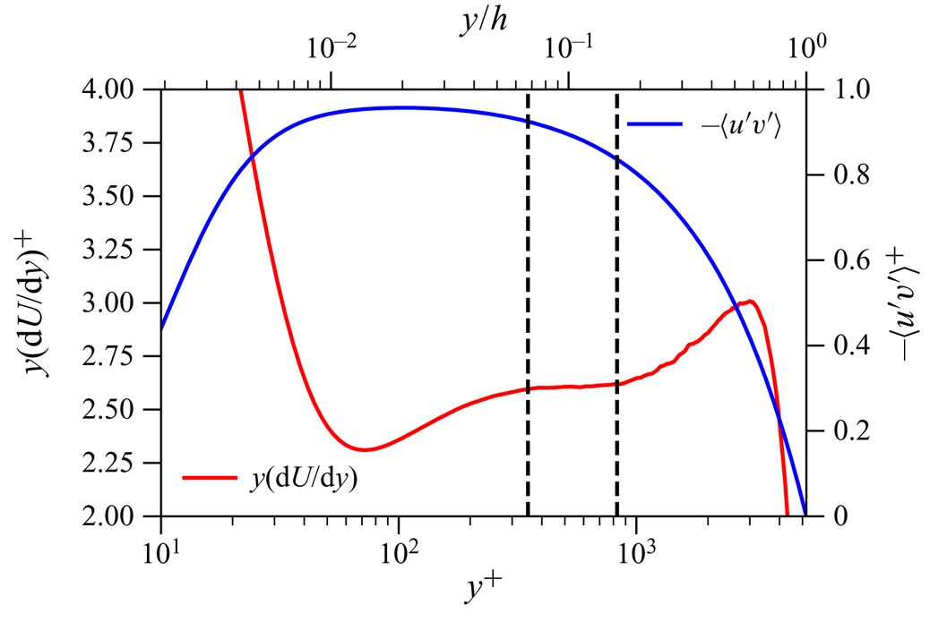
To demonstrate the validity of (2.6), the regions where the Reynolds shear stress is approximately constant and the mean velocity is approximately logarithmic (i.e.  $y^{+}\mathrm {d}U^{+}/\mathrm {d}y^{+}$ is approximately constant) are examined in figure 1. The region of
 $-\overline {u'v'}\simeq 1$ is located at
 $y^{+} \simeq 100$, whereas the one where
 $y^{+}\mathrm {d}U^{+}/\mathrm {d}y^{+}$ is approximately constant emerges a little above (
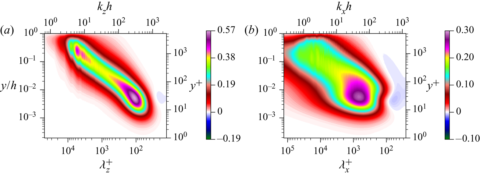
 $350 \delta _\nu \lesssim y \lesssim 0.16h$). Both spanwise and streamwise wavenumber spectra of the Reynolds shear stress shown in figure 2 suggest that
 $y^{+} \simeq 100$ would not be the best location where the self-similar scaling (2.6) is developed, as it is still under some non-negligible influence from the near-wall peak. Instead, the peak intensity of the premultiplied spectra at each wall-normal location is approximately constant in the region where
 $y^{+}\mathrm {d}U^{+}/\mathrm {d}y^{+}$ is approximately constant (see the spectral intensities along the ridge of figures 2a and 2b for
 $350 \delta _\nu \lesssim y \lesssim 0.16h$). The fact that (2.6) appears slightly above the peak wall-normal location of
 $-\overline {u'v'}$ is likely due to the Reynolds number of the DNS, which is still not high enough to directly compare with the asymptotic theory. Note that the maximum of
 $-\overline {u'v'}$ will occur at
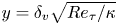 $y = \delta _v \sqrt {Re_\tau / \kappa }$, which is obtained by combining (1.1) with (2.1) (Afzal Reference Afzal1982; Morrison et al. Reference Morrison, McKeon, Jiang and Smits2004; Panton Reference Panton2007; Sillero, Jiménez & Moser Reference Sillero, Jiménez and Moser2013; Lee & Moser Reference Lee and Moser2015). Therefore, the maximum of
 $-\overline {u'v'}$ will be located in the region of
 $y \ge 350\delta _v$ when
 $Re_\tau \ge 47\,000$ with
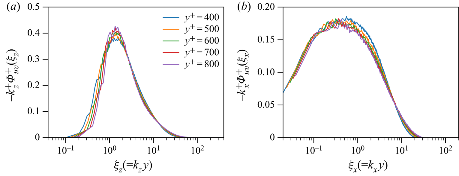
 $\kappa = 0.384$. However, given the scope of the present study and the further development of the analysis in § 3, it is more important to identify the wall-normal locations where the self-similarity of the Reynolds shear stress (2.6) is more precisely developed with the logarithmic mean velocity. Indeed, plotting
 $k \varPhi _{uv}$ in figure 3 with respect to the self-similar spanwise and streamwise wavenumbers (i.e.
 $\xi _z=k_z y$ and
 $\xi _x=k_x y$) confirms that (2.6) is approximately true in the region of
 $350 \delta _\nu \lesssim y \lesssim 0.16h$ where the mean velocity is close to a logarithmic with the von Kármán constant,
 $\kappa \simeq 0.384$ (Lee & Moser Reference Lee and Moser2015).
Test function for the logarithm in the mean velocity ( $y^{+}\mathrm {d}U^{+}/\mathrm {d}y^{+}$) and Reynolds shear stress. The data are from Lee & Moser (Reference Lee and Moser2015).

Contours of premultiplied Reynolds shear-stress (a) spanwise and (b) streamwise wavenumber co-spectra (from Lee & Moser Reference Lee and Moser2015).

Premultiplied Reynolds shear-stress co-spectra with respect to the similarity wavenumbers (a)  $\xi _z(=k_zy)$ and (b)
 $\xi _x(=k_xy)$ (from Lee & Moser Reference Lee and Moser2015).

3. Self-similarity of energy balance and the logarithmic mean
3.1. Energy balance in the logarithmic layer
While (2.6) provides a useful prediction for the self-similarity of the Reynolds shear stress, it does not carry any information for the mean velocity. Therefore, we shall proceed further by considering the equations for turbulent fluctuation:
 \begin{equation} \frac{\partial u_i^{\prime}}{\partial t}+U_j\frac{\partial u_i^{\prime}}{\partial x_j}=-{u_j^{\prime}} \frac{\partial U_i}{\partial x_j}+\frac{\partial}{\partial x_j} \left(-\frac{p^{\prime}}{\rho} \delta_{ij}-({u_i^{\prime}u_j^{\prime}}-\overline{u_i^{\prime}u_j^{\prime}})+ \nu\frac{\partial u_i^{\prime}}{\partial x_j}\right), \end{equation}
where  $p'$ is the pressure fluctuation. After taking the Fourier transform (2.4) to (3.1), multiplication by
 $\hat {u}^{*}_i$ and an average in time and the
 $r^{\bot }$-direction lead to the following equation for the spectral intensity of the total turbulent kinetic energy:
 \begin{align} 0 &\simeq \underbrace{\left\langle {\textrm{Re}} \left\{- \overline{\widehat{u^{\prime}}^{\ast} (y;k)\widehat{v^{\prime}}(y;k)} \frac{{\textrm d} U(y)}{{\textrm d} y} \right\} \right\rangle_{r^{\bot}}}_{\hat{P}\left( y;k \right)} -\underbrace{\left\langle \nu \overline{\frac{\partial{\widehat{u_{i}^{\prime}}(y;k)} }{\partial{x_{j}} } \frac{\partial{\widehat{u_{i}^{\prime}}^{\ast}(y;k)} }{\partial{x_{j}} }}\right\rangle_{r^{\bot}}}_{\hat{\epsilon}\left( y;k \right)} \nonumber\\ &\quad + \underbrace{\left\langle {\textrm{Re}} \left\{- \overline{\widehat{u_{i}^{\prime}}^{\ast}(y;k) \frac{\partial }{\partial{x_{j}} } \left( \widehat{ u_{i}^{\prime}u_{j}^{\prime} }(y;k) \right)}\right\}\right\rangle_{r^{\bot}}}_{\hat{T} \left( y;k \right)}, \end{align}
where  $\langle \cdot \rangle _{r^{\bot }}$ indicates an average in the
 ${r^{\bot }}$-direction. Here, the first term
 $\hat {P}$ in the right-hand side of (3.2) is the rate of turbulence production, the second term
 $\hat {T}$ is the rate of turbulent transport mostly representing the energy cascade, and the last term
 $\hat {\epsilon }$ is the rate of viscous dissipation. We note that, in (3.2), the wall-normal transport by pressure and viscous diffusion is ignored with the assumption of
 $y \gg \delta _\nu$, as it essentially originates from the no-slip boundary condition at the wall: indeed, the numerical simulation data have consistently shown that such wall-normal transport terms are quite small in the logarithmic layer (Cho, Hwang & Choi Reference Cho, Hwang and Choi2018; Lee & Moser Reference Lee and Moser2019). For the same reason, one would expect that
 $\int _0^{\infty } \hat {T}(y;k)\,\mathrm {d}k \simeq 0$ in the logarithmic layer due to the energy-conservative nature of the nonlinear term (see also figure 5). This implies that integration of (3.2) over
 $k$ yields the approximate balance between turbulence production and dissipation in the logarithmic layer (Tennekes & Lumley Reference Tennekes and Lumley1967): i.e.
 \begin{equation} P \simeq \epsilon, \end{equation}
where
 \begin{equation} P = \int_0^{\infty} \hat{P}(y;k)\,\mathrm{d}k \quad \mathrm{and}\quad \epsilon = \int_0^{\infty} \hat{\epsilon}(y;k)\,\mathrm{d}k. \end{equation}
It is worth noting that (3.3a) is valid only approximately in practice. Recent DNS studies of channel flows have shown that there is a subtle imbalance between production and dissipation in the logarithmic region, which slowly increases with  $Re_\tau$ (Lee & Moser Reference Lee and Moser2015). The non-zero
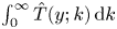 $\int _0^{\infty } \hat {T}(y;k)\,\mathrm {d}k$ is associated with the wall-normal transport of the imbalanced energy from the logarithmic to the near-wall region (Lee & Moser Reference Lee and Moser2019). Nonetheless, the turbulent energy transport
 $\hat {T}$ transferred across the wall-parallel wavenumbers is still significantly greater than that transferred in the wall-normal direction.
3.2. Logarithmic mean and self-similar energy balance
Now, we consider the energy balance given in (3.2) at the integral length scale, since the attached eddy hypothesis of Townsend (Reference Townsend1956, Reference Townsend1976) only concerns energy-containing eddies. In this case, the relevant regime of the wavenumber of interest should only be  $k \sim O(1/y)$, and the order of magnitude of each term in (3.2) is given by
 \begin{equation} \hat{P}\left( y;k\right) \sim O\left({u^{3}_\tau}\right),\quad \hat{T}\left( y;k\right)\sim O \left({u^{3}_\tau}\right),\quad \hat{\epsilon}\left( y;k \right) \sim O\left(Re^{-1}_y{u^{3}_\tau}\right), \end{equation}
where  $Re_y=Re_\tau y/h$. The approximate energy balance at
 $k \sim O(1/y)$ is then written as
 \begin{equation} \hat{P}+\hat{T} \simeq 0, \end{equation}
indicating that, at the integral scale, the turbulent energy production is approximately balanced with the turbulent transport due to the locally high Reynolds number  $Re_y$. It is evident that the turbulent transport term would transfer the energy produced at the integral scale to the Kolmogorov scale through the energy cascade (Kolmogorov Reference Kolmogorov1941). Here, we also note that the nature of slightly non-zero
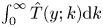 $\int _0^{\infty } \hat {T}(y;k) \mathrm {d}k$ does not affect (3.5) – it only affects (3.3). Combining (3.5) with (2.6) leads to the following energy balance at
 $k \sim O(1/y)$:
 \begin{equation} - \frac{f(\xi)}{k}\frac{{\textrm d} U}{{\textrm d} y} +\hat{T}\left(\, y;k \right) \simeq 0. \end{equation}
It is worth pointing out that (3.6) now contains the information of the mean shear, enabling us to relate the self-similarity at the integral scale to the mean velocity.
Let us now demonstrate that (3.6) admits a logarithmic mean velocity if and only if the energy balance in (3.6) is self-similar. First, we start by claiming that the energy balance at  $k \sim O(1/y)$ is self-similar. In other words, the turbulent transport term is claimed to be only a function of
 $\xi$:
 \begin{equation} \hat{T}\left(\, y;k_z \right) = g(\xi). \end{equation}
This then automatically makes the production  $\hat {P}$ only a function of
 $\xi$ from (3.6). Rearranging (3.6) subsequently yields
 \begin{equation} y\frac{{\textrm d} U}{{\textrm d} y} \simeq \frac{\xi g(\xi)}{f(\xi)}. \end{equation}
We note that the left-hand side of (3.8) is only a function of  $y$, while the right-hand side is only a function of
 $\xi$. Since
 $y$ and
 $k$ are independent of each other, so are
 $y$ and
 $\xi$. Therefore, the only possible way for (3.8) to be true would be if both sides are constant, resulting in
 \begin{equation} y \frac{{\textrm d} U(y)}{{\textrm d} y} \simeq C_0, \end{equation}
where  $C_0$ is the constant. This subsequently yields a logarithmic mean velocity:
 \begin{equation} U(y) \simeq C_0\ln y+C_1, \end{equation}
where  $C_1$ is a constant. It is even more straightforward to demonstrate that the inverse of this is true. If we claim (3.9) to be true, (3.6) gives
 \begin{equation} \hat{P}\left(\, y;k\right) \simeq -\frac{C_0}{\xi}f(\xi)\quad \textrm{and}\quad \hat{T}\left( y;k\right) \simeq \frac{C_0}{\xi}f(\xi), \end{equation}
indicating that the energy balance (3.5) is indeed only a function of  $\xi$ or is self-similar with respect to the distance from the wall
 $y$.
3.3. Numerical evidence
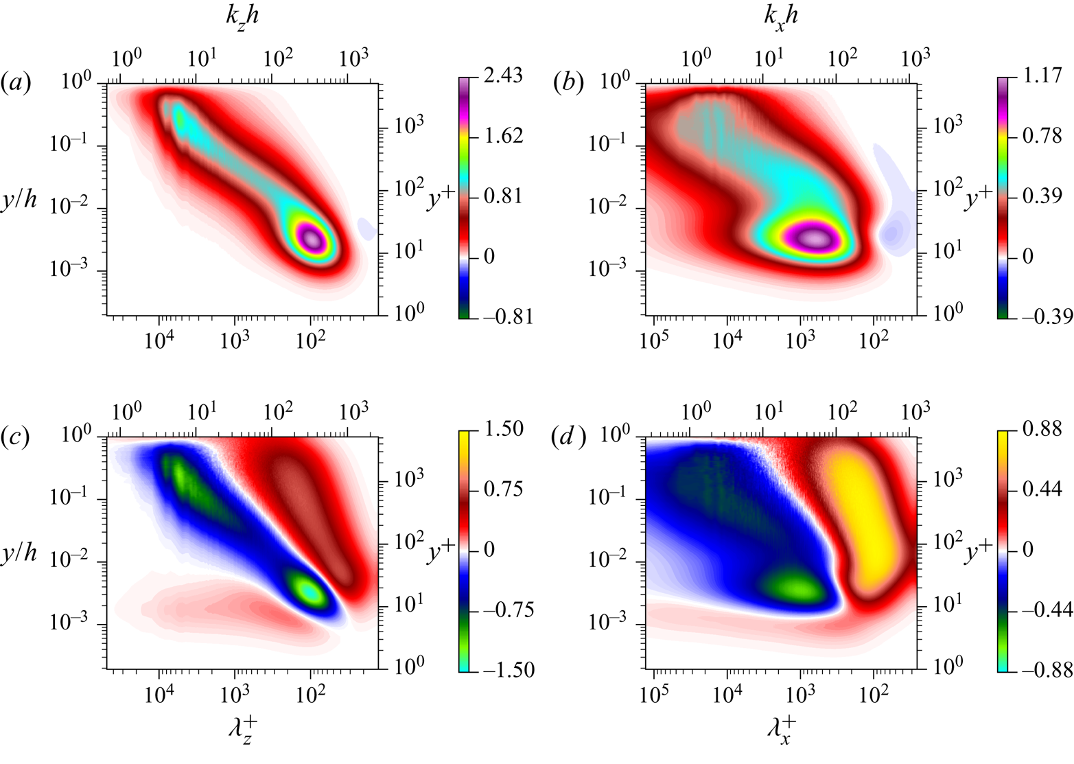
To verify the asymptotic theory in §§ 3.1 and 3.2, the premultiplied streamwise and spanwise wavenumber spectra of the rate of production ( $ky \hat {P}$) and turbulent transport (
 $ky \hat {T}$) are shown in figure 4. The production spectra are positive in most of the
 $k$–
 $y$ space (figures 4a,b). However, the turbulent transport spectra exhibit both positive and negative values from the energy-conservative nature of the turbulent transport (i.e.
 $\iint ky\hat {T} (y;k)\,\mathrm {d}(\ln k)\,\mathrm {d}(\ln y)=0$). We note that the contour shape of the positive production spectra appears to be very similar to that of the negative transport spectra. This implies that the turbulent transport takes most of the energy from the production and subsequently transfers it to the region where
 $\hat {T} (y;k)>0$ in the
 $k$–
 $y$ space for dissipation. The most obvious mechanism of this is the energy cascade (Kolmogorov Reference Kolmogorov1941): indeed, the region of
 $\hat {T} (y;k)>0$ with strong intensities appears for
 $k\gg O(y)$ (figures 4c,d), and it was shown to be aligned along
 $k\sim O(1/\eta )$ where
 $\eta =(y\delta _\nu ^{3})^{1/4}$ is the Kolmogorov length scale (Cho et al. Reference Cho, Hwang and Choi2018; Lee & Moser Reference Lee and Moser2019). In wall-bounded turbulence, it has also been found that
 $\hat {T} (y;k)>0$ appears with relatively weak intensities for
 $k\ll O(y)$. This region is located in the region close to the wall for very low
 $k$, and this was found to be associated with inverse energy transfer from small to large scale (e.g. Cho et al. Reference Cho, Hwang and Choi2018; Kawata & Alfredsson Reference Kawata and Alfredsson2018; Lee & Moser Reference Lee and Moser2019).
Contours of premultiplied spectral densities of the rate of (a,b) production ( $k^{+}y^{+}\hat {P}^{+}$) and (c,d) turbulent transport (
 $k^{+}y^{+}\hat {T}^{+}$) (from Lee & Moser Reference Lee and Moser2019): (a,c) spanwise and (b,d) streamwise wavenumber spectra.

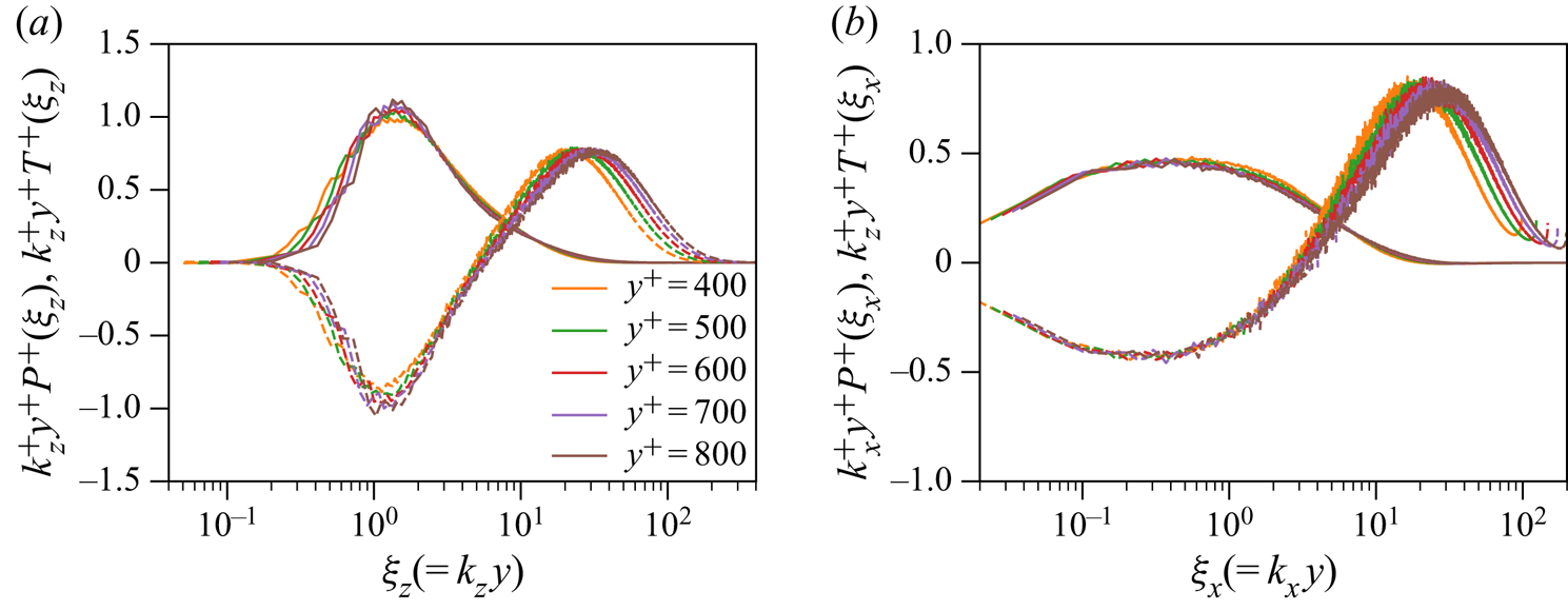
Finally, the self-similarity of the energy balance at  $k \sim O(1/y)$ for the logarithmic mean velocity is examined in figure 5. For the spanwise wavenumber spectra (figure 5a), (3.5) is approximately true for
 $\xi _z \sim 1$ (
 $\xi _z=k_z y$), and both
 $\hat {P}$ and
 $\hat {T}$ do follow the self-similar scaling given in (3.10a,b). Essentially the same happens in the streamwise wavenumber spectra (figure 5b) – the only difference from the spanwise wavenumber spectra is that (3.5) appears at
 $\xi _x \sim 0.1$ (
 $\xi _x=k_x y$), and this is presumably because the typical energy-containing eddies tend to be elongated in the streamwise direction with the scaling of
 $k_x \sim 0.1 k_z$ (Hwang Reference Hwang2015).
Premultiplied spectral densities of the rate of production (——) and turbulent transport (– – –) with respect to the self-similar wavenumbers (a)  $\xi _z(=k_zy)$ and (b)
 $\xi _x(=k_xy)$ (from Lee & Moser Reference Lee and Moser2019).

4. Concluding remarks
Starting from the self-similarity in the spectra of the Reynolds shear stress, in the present study we have analytically demonstrated that the mean velocity exhibits a logarithmic wall-normal dependence if and only if the balance of turbulent kinetic energy at the integral scale is self-similar with respect to the distance from the wall  $y$. This has then been verified with the DNS data of Lee & Moser (Reference Lee and Moser2015, Reference Lee and Moser2019). Given that the turbulent kinetic energy at the integral scale would statistically characterise energy-containing eddies in the flow, this analysis suggests that the existence of self-similar energy-containing eddies scaling with the distance from the wall would be a necessary and sufficient condition for the logarithmic mean velocity, providing direct theoretical grounds for the attached eddy hypothesis of Townsend (Reference Townsend1956, Reference Townsend1976).
It should also be mentioned that the most crucial assumption made in the present study is that the length scale in the logarithmic layer is the distance from the wall (von Kármán Reference von Kármán1931). In fact, if the length scale is chosen to be a fixed constant, every single element of the analysis from (2.2) can be replaced for homogeneous shear turbulence, resulting in a constant  $\textrm {d} U/ \textrm {d} y$. This is consistent with the simulation-based study of Mizuno & Jiménez (Reference Mizuno and Jiménez2013), who replaced the buffer layer with a suitably rescaled flow field from the region much farther from the wall. By doing so, they managed to retrieve the typical features of wall-bounded turbulence. It is evident that the rescaling procedure in their study artificially imposed the distance-from-the-wall scale on the simulation. Indeed, they also reported that if the rescaling procedure is removed from their simulation, they only obtain a homogeneous shear flow. Together with their numerical findings, the present study highlights the critical importance of the length scale given to the flow – as long as the distance-from-the-wall scale is imposed on the given system, it will reproduce many important features of wall turbulence. However, this should not be misinterpreted as meaning that the wall is not of the essence for the description of wall turbulence, because it is actually the wall which imposes the distance-from-the-wall scale. Finally, given the importance of the length scale imposed, the present analysis may well be improved further by incorporating a more precise form of the length scale (Klewicki Reference Klewicki2013), and this would remain future work.
Acknowledgements
Y.H. thanks Professor J. Klewicki for sharing a useful discussion during his visit to the University of Melbourne. Y.H. also thanks Professor I. Marusic for sharing the information about Perry & Abel (Reference Perry and Abel1975, Reference Perry and Abel1977) in relation to (2.6). Y. H. gratefully acknowledges the financial support of the Leverhulme Trust (RPG-2019-123), the Engineering and Physical Sciences Research Council (EPSRC; EP/T009365/1) in the UK, and the University of Melbourne through a visiting fellowship. This research used resources of the Argonne Leadership Computing Facility, which is a DOE Office of Science User Facility supported under Contract DE-AC02-06CH11357. Sandia National Laboratories is a multimission laboratory managed and operated by National Technology and Engineering Solutions of Sandia, LLC, a wholly owned subsidiary of Honeywell International, Inc., for the US Department of Energy's National Nuclear Security Administration under Contract DE-NA0003525. This paper describes objective technical results and analysis. Any subjective views or opinions that might be expressed in the paper do not necessarily represent the views of the US Department of Energy or the United States Government.
Declaration of interests
The authors report no conflict of interest.