





1. Introduction
Understanding and modelling turbulent flow in real-world systems ideally call for dense, time-resolved Eulerian fields: velocity, pressure, density and gradient tensors of the same. These fields allow one to educe coherent structures and superstructures (Schröder et al. Reference Schröder, Geisler, Sieverling, Wieneke, Henning, Scarano, Elsinga and Poelma2009; Schanz et al. Reference Schanz, Schröder, Gesemann, Huhn, Novara, Geisler, Manovski and Depuru-Mohan2018; Weiss et al. Reference Weiss, Schanz, Erdogdu, Schröder and Bosbach2023), quantify energy transfer and dissipation (Schneiders et al. Reference Schneiders, Scarano and Elsinga2017; Schröder et al. Reference Schröder, Schanz, Gesemann, Huhn, Garaboa-Paz and Bodenschatz2022), determine surface loading from pressure and shear stress (Rival & van Oudheusden Reference Rival and van Oudheusden2017; van Gent et al. Reference van Gent2017; Jux et al. Reference Jux, Sciacchitano and Scarano2020), analyse buoyancy-driven transport in convection (Muralidhar Reference Muralidhar2002; Wissink & Herlina Reference Wissink and Herlina2023) and so forth. In principle, scale-resolving computational fluid dynamics (CFD) methods can deliver such fields, but direct numerical simulation (DNS) becomes intractable when applied to device-scale flows at realistic Reynolds numbers (Slotnick et al. Reference Slotnick, Khodadoust, Alonso, Darmofal, Gropp, Lurie and Mavriplis2014; Cary et al. Reference Cary, Chawner, Duque, Gropp, Kleb, Kolonay, Nielsen and Smith2021), and large-eddy simulation depends on subgrid-scale closures that require tuning for new physical regimes (Argyropoulos & Markatos Reference Argyropoulos and Markatos2015; Duraisamy et al. Reference Duraisamy, Iaccarino and Xiao2019). Even in a small subdomain, accurate simulations hinge on the fidelity of boundary conditions that are often difficult to specify, such as representative upstream disturbances (Buchta et al. Reference Buchta, Laurence and Zaki2022; Johnson et al. Reference Johnson, Mysore, Schau and Oefelein2023), wall heat fluxes (Roy & Blottner Reference Roy and Blottner2006) or coherent structures in the inflow (Gorlé et al. Reference Gorlé, Garcia-Sanchez and Iaccarino2015; Xiao & Cinnella Reference Xiao and Cinnella2019). These boundaries are challenging to measure experimentally, and it is uncommon to set up CFD simulations using empirical unsteady boundary conditions.
Experiments, by contrast, capture the true behaviour of flows but yield measurements that are typically sparse, noisy and indirectly related to the quantities of interest. Data assimilation (DA) offers a means to combine these complementary capabilities: enforcing the governing equations via CFD methods while matching available measurements, thereby producing physically consistent reconstructions of real flows (He et al. Reference He, Li and Liu2025; Zaki Reference Zaki2025; Zaki & Wang Reference Zaki and Wang2025). In this context, Lagrangian particle tracking (LPT) (Schröder & Schanz Reference Schröder and Schanz2023) is an especially attractive diagnostic because it provides time-resolved, volumetric velocity and acceleration information in complex configurations and at high Reynolds numbers. The data, however, are limited to particle trajectories (also known as ‘tracks’) that are spatially sparse, subject to localisation and tracking errors, and, in some flows, whose velocities deviate from the underlying fluid velocity due to particle inertia. This leads to the central question motivating our study: Given experimentally realisable Lagrangian data, to what extent can we recover the antecedent sequence of Eulerian flow states and salient particle properties, such as their true positions, sizes and densities, by supplementing the tracks with the equations of motion for the carrier and particle phases in a DA reconstruction?
1.1. Capabilities and limitations of Lagrangian particle tracking
Lagrangian particle tracking has emerged as a leading diagnostic for volumetric velocimetry in both laboratory and field environments (Bristow et al. Reference Bristow, Li, Hartford, Guala and Hong2023; Li et al. Reference Li, Guala and Hong2024; Schröder et al. Reference Schröder, Schanz, Geisler, Godbersen, Agocs and Simhan2024). Compared with tomographic particle image velocimetry (PIV) (Scarano Reference Scarano2012), it achieves higher spatial resolution and nearly ghost-free particle fields, enabling more accurate computation of derivatives and more reliable pressure inference (van Gent et al. Reference van Gent2017). Tracks are obtained by seeding the flow with tracer particles (or by leveraging natural tracers), imaging them with one or more cameras and reconstructing three-dimensional (3-D) particle positions before linking them in time. Multi-camera triangulation provides high-accuracy localisation from overlapping views, while single-camera methods such as digital in-line holography (DIH) (Toloui et al. Reference Toloui and Hong2015; Mallery et al. Reference Mallery and Hong2019), plenoptic cameras (Fahringer et al. Reference Fahringer, Lynch and Thurow2015; Hall et al. Reference Hall, Guildenbecher and Thurow2017) or defocusing imaging (Guo et al. Reference Guo, Ardekani and Vlachos2019) enable four-dimensional measurements in settings where optical access is limited. Recent advances, including the predictor–corrector approach of shake-the-box (STB) tracking (Schanz et al. Reference Schanz, Gesemann and Schröder2016; Schröder et al. Reference Schröder, Schanz, Geisler, Godbersen, Agocs and Simhan2024), object-aware LPT near boundaries (Wieneke & Rockstroh Reference Wieneke and Rockstroh2024), field-scale deployments in atmospheric turbulence (Bristow et al. Reference Bristow, Li, Hartford, Guala and Hong2023; Li et al. Reference Li, Guala and Hong2024) and multi-pulse schemes for high-speed compressible flows (Novara et al. Reference Novara, Schanz, Geisler, Gesemann, Voss and Schröder2019; Manovski et al. Reference Manovski, Novara, Mohan, Geisler, Schanz, Agocs, Godbersen and Schröder2021), have expanded the technique’s reach. Hence, LPT is now frequently applied to flows of practical relevance.
Two challenges are especially relevant to the question of what can be inferred from LPT data. The first challenge is localisation and tracking error. Although present in all LPT variants, these errors are most severe for single-camera systems (i.e. based on plenoptic or DIH imaging), which suffer from strongly anisotropic uncertainties due to depth-of-focus limitations. The largest errors occur along the optical axis (Katz & Sheng Reference Katz and Sheng2010; Gao et al. Reference Gao, Guildenbecher, Reu and Chen2013), degrading velocity estimates and, in turn, derived quantities such as vorticity and pressure. The second challenge is inertial transport. Particles with finite response times, characterised by their Stokes number
 $\textit{St} = \tau _{\!{p}}/\tau _{\!{f}}$
, where
 $\tau _{\!{p}}$
and
 $\tau _{\!{f}}$
are characteristic time scales of the particle and carrier fluid, deviate systematically from the local fluid velocity (Melling Reference Melling1997; Raffel et al. Reference Raffel, Willert, Scarano, Kähler, Wereley and Kompenhans2018). While small particles, with
 $\textit{St} \lt 0.1$
, are used to ensure good ‘traceability’ in LPT, inertial particle transport may occur inadvertently in both laboratory and natural settings. Examples include helium-filled soap bubbles in wind tunnels (Wolf et al. Reference Wolf, Schwarz, Kaufmann, Gardner, Michaelis, Bosbach, Schanz and Schröder2019; Faleiros et al. Reference Faleiros, Tuinstra, Sciacchitano and Scarano2021), solid particles in shocked flows (Ragni et al. Reference Ragni, Schrijer, van Oudheusden and Scarano2011), snowflakes in the atmospheric boundary layer (Li et al. Reference Li, Guala and Hong2022; Bristow et al. Reference Bristow, Li, Hartford, Guala and Hong2023) and sediment transport in waterways (Righetti & Romano Reference Righetti and Romano2004), with
 $\textit{St}$
varying from 0.1 to 10 in these examples. Track errors and particle inertia seemingly reduce the information content of LPT data and thus prevent the accurate determination of flow fields from particle tracks in a typical LPT workflow.
1.2. Data assimilation for Lagrangian particle tracking
Early reconstruction approaches for LPT converted Lagrangian tracks into Eulerian fields by interpolation (Agüí & Jimenez Reference Agüí and Jimenez1987; Malik & Dracos Reference Malik and Dracos1995), but these methods were limited by the particle sampling resolution and prone to amplifying noise. Modern DA methods incorporate the Navier–Stokes equations as constraints, either as hard constraints (ensemble Kalman filters (Deng et al. Reference Deng, He, Wen and Liu2018); adjoint–variational methods (Gronskis et al. Reference Gronskis, Heitz and Mémin2013; Foures et al. Reference Foures, Dovetta, Sipp and Schmid2014; He et al. Reference He, Zeng, Wang, Wen and Liu2024)) or as soft ones (physics-based interpolation with B-splines (Gesemann et al. Reference Gesemann, Huhn, Schanz and Schröder2016); radial basis functions (Casa & Krueger Reference Casa and Krueger2013); vorticity formulations (Jeon et al. Reference Jeon, Schneiders, Müller, Michaelis and Wieneke2018)). By enforcing physical consistency, these methods have the potential to reconstruct velocity fields beyond the limits of interpolation per se, recovering information at scales finer than the particle-sampling Nyquist wavenumber (though this has yet to be demonstrated experimentally). Machine learning variants, like those based on physics-informed neural networks (PINNs) (Raissi et al. Reference Raissi, Perdikaris and Karniadakis2019), offer flexible functional representations and have been successfully applied to a broad range of flows. They are increasingly relied upon for LPT DA, including in the present study, owing to their ease of implementation, robustness in inverse settings and demonstrated accuracy with sparse or noisy data (Zhou et al. Reference Zhou, Grauer, Schanz, Godbersen, Schröder, Rockstroh, Jeon and Wieneke2024).
Two central difficulties remain when processing LPT data, stemming from the challenges introduced above. One is localisation and tracking errors, which directly limit the fidelity of reconstructed velocities; these errors can be compounded by biases which are inadvertently introduced during track filtering. The other is the assumption of ideal tracers, which breaks down when particles have non-negligible inertia, creating the additional challenge of jointly inferring particle properties alongside flow fields. In other words, the particle–flow coupling must be modelled to reconstruct the flow, and it is not known a priori whether carrier-phase flow fields and particle properties can be jointly determined from LPT track data. A related theoretical question is whether the same framework can also recover the true particle positions from noisy measurements. Although this is rarely a primary objective in LPT, since particle positions are merely a means to recover flow fields, successful recovery of the true positions from noisy data would indicate that the governing physics and the measurements jointly constrain the track geometries, highlighting the information content of Lagrangian data in turbulence. Addressing these challenges requires a DA framework that treats particle positions as the measured quantity rather than velocities, encodes the coupled carrier-phase and particle-phase dynamics and operates directly on noisy particle position data. The development and demonstration of such a framework is one focus of this work.
1.3. Present approach and investigations of joint estimation
We empirically demonstrate the feasibility of jointly estimating flow fields and particle properties using a framework that we term neural-implicit particle advection (NIPA). The NIPA framework couples an Eulerian flow model, parametrised by coordinate neural networks (i.e. PINNs when trained with a physics loss), to individual Lagrangian particle models that embed the particle advection equation as a hard constraint. For inertial particles, their size, density and other attributes enter the model as trainable parameters, enabling estimation of properties that determine their response times. The governing physics enter via soft constraints on the Navier–Stokes equations for the carrier phase and an extended Maxey–Riley formulation for the particle (or ‘disperse’) phase (Subramaniam & Balachandar Reference Subramaniam and Balachandar2022). By design, NIPA works directly from the raw track positions, avoiding any biases induced by filtering the tracks, and it estimates both flow states and particle properties without requiring direct observations of either.
The NIPA framework provides numerical means to assess the factors that govern reconstruction accuracy across a range of flow regimes and measurement conditions. Moreover, it represents an algorithmic advance in LPT DA. We probe the degree to which flow fields can be recovered from Lagrangian data through synthetic test cases that include noisy tracks from ideal tracers in incompressible turbulence, inertial particles in the same and inertial particles in a compressible flow with a shock wave. In each case, we examine whether the available track data and governing equations suffice to recover the flow field and particle properties, and we study the sensitivity of reconstruction accuracy to the seeding density, noise level and Stokes number. These results provide empirical evidence for the existence of an inverse mapping from a Lagrangian measurement manifold to a flow’s global attractor in state space. Despite the empirical nature of this work, our findings motivate a formal analysis of the joint observability of flow–particle systems (Zaki Reference Zaki2025). The remainder of this paper outlines the reconstruction methodology in § 2, describes the flow cases used for numerical testing in § 3 and the implementation details in § 4, tests the joint estimation of particle positions for ideal tracers in § 5 and extends this treatment to inertial particles for turbulent and compressible flow reconstruction in § 6. Lastly, in § 7, we investigate the sensitivity of reconstruction accuracy to both particle inertia and noise before concluding the paper in § 8.
2. Methodology: neural-implicit particle advection
Understanding when flow fields and particle properties can be jointly recovered from Lagrangian data requires a DA algorithm that accounts for the physics of both phases. Existing DA methods either reconstruct the flow but treat the particles as ideal tracers, neglecting particle–fluid interactions, or they infer the particle dynamics given full knowledge of the flow field (Domínguez-Vázquez et al. Reference Domínguez-Vázquez, Escobar-Castaneda, Wang and Jacobs2025). Neither approach is adequate to the task at hand. To remedy this shortcoming, we introduce a new framework for LPT DA, which we call NIPA. It features dedicated models of both the flow and the particles, which are coupled through the governing equations of disperse multiphase flow, namely the Navier–Stokes and extended Maxey–Riley equations. By simultaneously optimising the flow and particle models to satisfy these equations, NIPA recovers not only time-resolved flow fields but also enhanced particle trajectories and otherwise unknown particle properties. This tool thus enables the systematic evaluation of how dataset attributes (e.g. the number and spacing of particles, data fidelity, particle inertia and compressibility) affect reconstruction accuracy. Below, we present our framework, define the objective loss terms and describe our flow and particle models.
2.1. Framework for data assimilation
The NIPA framework employs ‘neural-implicit flow states’ coupled to a set of particle models, with one model per particle, to reconstruct unsteady flow fields from Lagrangian tracks. A schematic of the approach is shown in figure 1. The flow field is represented using one or more coordinate neural networks, which take space–time input coordinates and return flow variables at that position and time:
 \begin{equation} \mathsf{F} : \mathcal{V} \times \mathcal{T} \rightarrow \mathbb{R}^{d+1}, \quad \left (\boldsymbol{x}, t\right ) \mapsto \left (\boldsymbol{u}, p\right )\!, \end{equation}
where
 $\boldsymbol{x} \in \mathcal{V}$
are the spatial coordinates in the flow domain
 $\mathcal{V}$
,
 $t \in \mathcal{T}$
is a time within the measurement interval
 $\mathcal{T}$
,
 $\boldsymbol{u}$
and
 $p$
are the velocity and pressure fields, respectively, and
 $d = 2$
or 3 is the number of spatial dimensions. Additional variables can be added to the outputs of
 $\mathsf{F}$
as needed, such as density or temperature in compressible flows. When coordinate neural networks like
 $\mathsf{F}$
are trained to minimise residuals to a set of physical equations, they are deemed to be PINNs. Network architectures used in this work are described in more detail in § 2.3.
Architecture of the neural DA solver. Eulerian flow fields are represented by one or more neural networks. Fourier encoding (FE) enhances network expressivity and broadband spectral coverage. Each particle is represented by a Lagrangian kinematics-constrained track (KCT) model. Flow fields, particle kinematics and particle properties (when
 $\textit{St} \gt 0$
) are jointly inferred from the data and governing equations.

We next introduce the concept of our Lagrangian particle model, whose detailed formulation is derived in § 2.4. Measured particle tracks natively comprise sequences of spatial positions determined at the image times. Accordingly, our particle models are defined with respect to these tracked locations, which may be adjusted during training to account for localisation uncertainty. For the
 $k$
th particle, a dedicated model
 ${\mathsf{P}}^{\kern-1pt(k)}$
is built to represent its velocity as a continuous function of time:
 \begin{equation} {\mathsf{P}}^{\kern-1pt(k)} : {\mathcal{T}}^{\,(k)} \rightarrow \mathbb{R}^d, \quad t \mapsto {\boldsymbol{v}}^{\kern-1pt(k)} \quad \text{for}\quad k \in \{1, \ldots , n_{\!{p}}\}, \end{equation}
where
 ${\boldsymbol{v}}^{\kern-1pt(k)}$
is the velocity of particle
 $k$
at time
 $t \in {\mathcal{T}}^{\,(k)}$
,
 ${\mathcal{T}}^{\,(k)} \subseteq \mathcal{T}$
is the time span of that track and
 $n_{\!{p}}$
is the total number of particle tracks. Although
 ${\mathsf{P}}^{\kern-1pt(k)}$
may take various forms, a physical track model must satisfy both kinematic and dynamic constraints. Kinematic consistency corresponds to an advection equation:
 \begin{equation} {\boldsymbol{x}_{\!j}}^{\kern-1pt(k)} - {\boldsymbol{x}_{\!j-1}}^{\kern-1pt(k)} = \int _{t_{\!j-1}}^{t_{\!j}} {\boldsymbol{v}}^{\kern-1pt(k)}\mathopen {} \left (t\right ) \,\mathrm{d}t \quad \text{for}\quad j \in \{1, \ldots , n_k-1\}, \end{equation}
where
 ${\boldsymbol{x}_{\!j}}^{\kern-1pt(k)}$
is the position of particle
 $k$
at the
 $j$
th time step
 $t_{\!j}$
and
 $n_k$
is the number of measurement points along that track. We embed this advection equation (2.3) as a hard constraint into
 ${\mathsf{P}}^{\kern-1pt(k)}$
, as elaborated in § 2.4. The dynamic consistency of
 ${\mathsf{P}}^{\kern-1pt(k)}$
is weakly enforced by the physics-based optimisation described in § 2.2.
Our formulation of
 ${\mathsf{P}}^{\kern-1pt(k)}$
provides a general framework for modelling the kinematics of both ideal tracers and inertial particles. In the latter case, properties of inertial particles like their size, density and shape determine
 $\tau _{\!{p}}$
and govern the particles’ coupling to the carrier fluid (Subramaniam & Balachandar Reference Subramaniam and Balachandar2022). These properties, and hence any slip velocities, are nearly always unknown in practice, complicating the reconstruction problem. To address this, we treat the relevant particle properties as model parameters to be learned, enabling the implicit characterisation of particles from LPT data in conjunction with the equations of motion for both phases. In well-characterised experiments, by contrast, where the pertinent particle properties are known prior to reconstruction, they may be fixed in the model.
2.2. Composite objective function
Flow and particle states ought to satisfy the governing equations for both phases, they must match known boundary conditions and they should be consistent with the observed LPT data. To achieve these objectives, the flow model
 $\mathsf{F}$
and particle models
 ${\mathsf{P}}^{\kern-1pt(k)}$
are trained in tandem by minimising a composite loss:
 \begin{equation} \mathscr{J}_{\textit{total}} = \chi _1 \mathscr{J}_{\textit{data}}^{\,\boldsymbol{x}} + \chi _2 \,\mathscr{J}_{\textit{phys}}^{\,\textit{flo}w} + \chi _3 \,\mathscr{J}_{\textit{phys}}^{\,\textit{part}} + \chi _4 \,\mathscr{J}_{\textit{bound}}, \end{equation}
where
 $\chi _i$
are weighting coefficients that balance the relative contributions of each term. The four loss terms, detailed below, are the position-based data fidelity term
 $\mathscr{J}_{\textit{data}}^{\,\boldsymbol{x}}$
(cf. the velocity-based term in § 2.2.4), the flow physics term
 $\mathscr{J}_{\mathrm{phys}}^{\,\textit{flo}w}$
, the particle physics term
 $\mathscr{J}_{\textit{phys}}^{\,\textit{part}}$
and the boundary condition term
 $\mathscr{J}_{\textit{bound}}$
.
2.2.1. Data fidelity loss
Particle positions are treated as trainable parameters, meaning that the estimated position of each particle at each measurement time can be adjusted during reconstruction. Without additional constraints, however, allowing the particles to move risks unmooring the models from the measurements. To anchor reconstructions to the experiment, therefore, we introduce a data fidelity term that penalises discrepancies between measured and estimated positions, weighted by the localisation uncertainty:
 \begin{equation} \mathscr{J}_{\textit{data}}^{\,\boldsymbol{x}} = \left ( \frac {1}{{ d} n_{\!{p}}} \sum _{k=1}^{n_{\!{p}}} \frac {1}{n_k} \sum _{i=1}^{n_k} {\underbrace {\left \lVert {\boldsymbol{x}_{i}}^{\kern-1pt(k)} - {\widehat {\boldsymbol{x}}_{i}}^{\kern-1pt(k)} \right \rVert _{\unicode{x1D647}}^2}_{\text{chi-squared statistic}}} - 1 \right )^2\!. \end{equation}
Here,
 ${\boldsymbol{x}_i}^{\kern-1pt(k)}$
and
 ${\widehat {\boldsymbol{x}}_i}^{\kern-1pt(k)}$
are the measured and estimated (i.e. trainable) positions of the
 $k$
th particle at time
 $t_i$
, with
 $n_{\!{p}}$
total tracks and
 $n_k$
samples in the
 $k$
th track. The norm is the matrix-weighted Mahalanobis norm:
 \begin{align} \left \lVert \Delta \boldsymbol{x} \right \rVert _{\unicode{x1D647}}^2 = \Delta \boldsymbol{x}^\top\unicode{x1D647}^\top\unicode{x1D647} \Delta \boldsymbol{x}, \quad \text{where}\quad\unicode{x1D647}^\top\unicode{x1D647} = \boldsymbol{\varGamma }^{-1} \end{align}
and
 $\boldsymbol{\varGamma }$
is the covariance matrix for the localisation errors. For independent, centred Gaussian errors, the weighted norm follows a chi-squared distribution with
 $d$
degrees of freedom, where
 $d$
is the dimension of
 $\boldsymbol{x}$
and also the expected value of the statistic. Normalising the chi-squared statistic by
 $d$
, subtracting 1 and squaring the result, as in (2.5), encourages consistency of the residuals
 $\lVert {\boldsymbol{x}_{i}}^{\kern-1pt(k)} - {\widehat {\boldsymbol{x}}_{i}}^{\kern-1pt(k)}\rVert _2$
with the expected statistics of the localisation errors. Values below
 $d$
are indicative of overfitting to noise, while values above
 $d$
suggest underfitting. In isolation, (2.5) acts as a maximum likelihood criterion for the particle positions. Notably, there exists an infinite set of minimisers for (2.5) for any set of LPT data. When coupled with the physics and boundary losses, however, the data loss enables a physics-informed particle tracking method. Both uses of (2.5) are demonstrated in § 5.
2.2.2. Physics-based loss terms
The flow physics loss penalises residuals of the carrier-phase governing equations:
 \begin{equation} \mathscr{J}_{\textit{phys}}^{\,\textit{flo}w} = \frac {\dim (\boldsymbol{e}_{\!{f}})^{-1}}{\left |\mathcal{V} \times \mathcal{T}\right |} \int _{\mathcal{T}} \int _{\mathcal{V}} \left \lVert \boldsymbol{e}_{\!{f}} \right \rVert _2^2 \mathrm{d}\boldsymbol{x} \,\mathrm{d}t, \end{equation}
where
 $\boldsymbol{e}_{\!{f}}$
is the residual vector associated with the governing flow equations within
 $\mathcal{V} \times \mathcal{T}$
. For domains with transient boundaries, the space–time domain is not the simple Cartesian product of
 $\mathcal{V}$
and
 $\mathcal{T}$
; see Tang et al. (Reference Tang, Zhou, Tan and Grauer2026) for details on handling such situations. While most LPT DA algorithms are restricted to incompressible flows, the present framework can be extended to compressible configurations with minimal modification. Appendix A summarises the governing equations used in this study.
The particle physics loss is based on residuals from an equation of motion for the disperse phase:
 \begin{equation} \mathscr{J}_{\textit{phys}}^{\,\textit{part}} = \frac {\dim \mathopen {} ( {\boldsymbol{e}_{\!{p}}})^{-1}}{n_{\!{p}}} \sum _{k=1}^{n_{\!{p}}} \frac {1}{|{\mathcal{T}}^{\,(k)}|} \int _{{\mathcal{T}}^{\,(k)}} \big \lVert {\boldsymbol{e}_{\!{p}}}^{\kern-1pt(k)}\big \rVert _2^2 \mathrm{d}t, \end{equation}
where
 ${\boldsymbol{e}_{\!{p}}}^{\kern-1pt(k)}$
is the residual of the
 $k$
th particle’s governing equation. For small spherical particles with a vanishing particle Reynolds number, the dynamics is described by the Maxey–Riley equation (Maxey & Riley Reference Maxey and Riley1983; Capecelatro & Wagner Reference Capecelatro and Wagner2023). The specific form adopted in this work, including its adaptation for compressible flows, is summarised in Appendix B. In cases with inertial particle transport, information about particle properties is obtained through the residuals in (2.8), since the equation of motion (and therefore
 ${\boldsymbol{e}_{\!{p}}}^{\kern-1pt(k)}$
) generally depends on the flow velocity
 $\boldsymbol{u}$
, the particle velocity
 ${\boldsymbol{v}}^{\kern-1pt(k)}$
and particle characteristics such as their sizes and densities.
In many LPT experiments, the particles are carefully selected to behave as ideal tracers with negligible slip velocities. In the limit
 $\textit{St} \to 0$
, the particle and carrier motions are equal. Hence, we specify velocity and acceleration residuals for ideal tracers:
 \begin{equation} {\boldsymbol{e}_{\!{p}, \boldsymbol{u}}}^{\kern-1pt(k)} = \boldsymbol{u} - {\boldsymbol{v}}^{\kern-1pt(k)} \quad \text{and}\quad {\boldsymbol{e}_{\!{p}, \boldsymbol{a}}}^{\kern-1pt(k)} = \frac {\mathrm{D}\boldsymbol{u}}{\mathrm{D}t} - {\boldsymbol{a}}^{\kern-1pt(k)}, \end{equation}
where
 $\mathrm{D}/\mathrm{D}t$
is the material derivative operator,
 ${\boldsymbol{a}}^{\kern-1pt(k)}$
is the acceleration of a particle and
 $\boldsymbol{e}_{\!{p}}$
is the concatenation of
 $\boldsymbol{e}_{\!{p}, \boldsymbol{u}}$
and
 $\boldsymbol{e}_{\!{p}, \boldsymbol{a}}$
.
2.2.3. Boundary condition loss
Although neural state estimation does not explicitly require boundary conditions, incorporating known constraints can improve reconstruction accuracy. In turbulent boundary layers (TBLs), for instance, enforcing a no-slip condition at the wall enhances near-wall resolution, where positional uncertainties are worsened by optical reflections and where the flow scales are smallest. This combination of large relative uncertainty and fine-scale dynamics makes boundary conditions especially valuable near walls. The no-slip boundary loss is
 \begin{equation} \mathscr{J}_{\textit{bound}} = \frac {\dim (\boldsymbol{u})^{-1}}{\left |\mathcal{A} \times \mathcal{T}\,\right |} \int _{\mathcal{T}} \int _{\mathcal{A}} \left \lVert \boldsymbol{u} \right \rVert _2^2 \,\mathrm{d}\boldsymbol{x} \,\mathrm{d}t, \end{equation}
where
 $\mathcal{A} \subseteq \partial \mathcal{V}$
denotes the no-slip portion of the domain boundary
 $\partial \mathcal{V}$
. This formulation can be extended to moving-wall conditions (Tang et al. Reference Tang, Zhou, Tan and Grauer2026), enabling the inference of wall motion, or to hybrid constraints that feature multiple variables (e.g. a constant free-stream density, adiabatic walls, or known pressures at tap locations) and boundary types (Dirichlet, Neumann, Robin), depending on the pertinent physics.
2.2.4. Baseline flow-only reconstruction
To evaluate the added value of joint flow–particle reconstruction, we implement a simplified baseline that neglects the particle models and instead relies on velocity information derived from the particle tracks through an intermediate step, as is common in LPT DA (Di Leoni et al. Reference Di Leoni, Agarwal, Zaki, Meneveau and Katz2023; Shin & Schröder Reference Shin and Schröder2025). In this baseline, the framework reduces to a flow network
 $\mathsf{F}$
that is trained to reproduce the track-based velocity estimates
 $\widehat {\boldsymbol{v}}$
while satisfying the governing equations and boundary conditions. The corresponding loss is
 \begin{equation} \mathscr{J}_{\textit{total}} = \chi _1 \mathscr{J}_{\textit{data}}^{\,\boldsymbol{u}} + \chi _2 \mathscr{J}_{\textit{phys}}^{\,\textit{flo}w} + \chi _3 \mathscr{J}_{\textit{bound}}, \end{equation}
where
 $\mathscr{J}_{\textit{data}}^{\,\boldsymbol{u}}$
enforces agreement between the reconstructed flow velocity and particle velocities inferred from the tracks. The velocity-based data fidelity term is
 \begin{equation} \mathscr{J}_{\textit{data}}^{\,\boldsymbol{u}} = \frac {1}{n_{\!{p}}} \sum _{k=1}^{n_{\!{p}}} \frac {1}{n_k} \sum _{i=1}^{n_k} \big \lVert \boldsymbol{u} - {\widehat {\boldsymbol{v}}_{i}}^{\kern-1pt(k)} \big \rVert _2^2, \end{equation}
where
 $\boldsymbol{u}$
is the velocity field from
 $\mathsf{F}$
and
 ${\widehat {\boldsymbol{v}}_{i}}^{\kern-1pt(k)}$
is the velocity estimate for the
 $k$
th particle at time
 $t_i$
. Such estimates may be obtained by differentiating the tracked positions, but finite differencing amplifies noise, so smoothing or interpolation schemes like those based on B-splines, polynomial fits or kernel convolution are often applied. Here, we demonstrate ‘baseline reconstructions’ using both a second-order finite-difference scheme (with single-sided differences at the track ends) and a quasi-optimal B-spline filter, detailed in Appendix C. While these methods can suppress the effects of noise in
 ${\widehat {\boldsymbol{v}}_{i}}^{\kern-1pt(k)}$
, they also embed errors in
 $\mathscr{J}_{\textit{data}}^{\,\boldsymbol{u}}$
through the heuristic choice of filter parameters. By contrast, our position-based formulation in (2.5) and the associated particle models bypass the intermediate estimation of velocity. Instead, we anchor the reconstruction to the measured positions, subject to the localisation error statistics.
We wish to emphasise that this ‘velocity data loss’ formulation is used solely as a baseline. It represents the performance attainable when particle–fluid coupling and particle properties are ignored, thereby highlighting the added value of joint estimation.
2.3. Neural flow model
The flow model consists of one or more neural networks, here denoted by
 $\mathsf{F}$
, comprising an input layer, output layer and
 $n_{{L}}$
hidden layers:
 \begin{equation} {\boldsymbol{z}}^{(n_{{L}}+1)} = \mathsf{F}\mathopen {} \big ({\boldsymbol{z}}^{(0)}\big) = \unicode{x1D652}^{\,(n_{{L}}+1)} \big [{\mathsf{L}}^{(n_{{L}})} \circ {\mathsf{L}}^{(n_{{L}}-1)} \circ \cdots \circ {\mathsf{L}}^{(2)} \circ \mathsf{G}\mathopen {}\big ({\boldsymbol{z}}^{(0)}\big )\big ] + {\boldsymbol{b}}^{(n_{{L}}+1)}, \end{equation}
with
 \begin{equation} {\boldsymbol{z}}^{(L)} = \mathsf{L}^L\mathopen {}\big ({\boldsymbol{z}}^{(L-1)}\big) = \text{swish}\mathopen {} \big ({\unicode{x1D652}}^{\,(L)} {\boldsymbol{z}}^{(L-1)} + {\boldsymbol{b}}^{(L)}\big ), \quad \text{for}\quad L \in \{2, \ldots , n_{{L}}\}. \end{equation}
In this expression,
 ${\boldsymbol{z}}^{(L)}$
are the outputs at layer
 $L$
and
 $\mathsf{L}$
represents the operator that maps between consecutive hidden layers. This operator consists of an affine transform followed by a nonlinear activation that is applied element-wise. The matrix
 ${\unicode{x1D652}}^{\,(L)}$
and the vectors
 ${\boldsymbol{b}}^{(L)}$
are the weights and biases of the affine transform, respectively; the latter provides an additive offset at each layer (not to be confused with measurement or estimation biases). We use the swish activation
 \begin{equation} \text{swish}(z_i) = \frac {z_i \,\exp (z_i)}{1 + \exp (z_i)}, \end{equation}
which has been shown to mitigate issues associated with vanishing gradients and is also smooth, making it well suited for representing flow fields that must be at least twice differentiable (Jagtap & Karniadakis Reference Jagtap and Karniadakis2023). Furthermore, to mitigate the low-frequency bias that commonly occurs in gradient-based training (Wang et al. Reference Wang, Teng and Perdikaris2021), the first hidden layer
 ${\mathsf{L}}^{(1)}$
is replaced by a Fourier encoding
 $\mathsf{G}$
(Tancik et al. Reference Tancik, Srinivasan, Mildenhall, Fridovich-Keil, Raghavan, Singhal, Ramamoorthi, Barron and Ng2020):
 \begin{align} {\boldsymbol{z}}^{(1)} = \mathsf{G}\mathopen {}\big ({\boldsymbol{z}}^{(0)}\big) = \Big [\sin \mathopen {}\big(2\pi \boldsymbol{f}_1 \boldsymbol{\cdot } {\boldsymbol{z}}^{(0)}\big), \,\cos \mathopen {}\big(2\pi \boldsymbol{f}_1 \boldsymbol{\cdot } {\boldsymbol{z}}^{(0)}\big), \ldots , \,\sin \mathopen {}\big(2\pi \boldsymbol{f}_{n_{\!{f}}} \boldsymbol{\cdot } {\boldsymbol{z}}^{(0)}\big), \,\cos \mathopen {}\big(2\pi \boldsymbol{f}_{n_{\!{f}}} \boldsymbol{\cdot } {\boldsymbol{z}}^{(0)}\big)\Big ], \end{align}
where
 $\boldsymbol{f}_{\!i}$
are random frequency vectors, sampled once upon initialisation and fixed during training, and
 $n_{\!{f}}$
is the number of features. For an incompressible flow represented by a single network, the input is
 ${\boldsymbol{z}}^{(0)} = (\boldsymbol{x}, t)$
and the output is
 ${\boldsymbol{z}}^{(n_{{L}}+1)} = (\boldsymbol{u}, p)$
.
Two additional strategies are used to improve reconstruction accuracy. First, some flow variables (e.g. density, temperature, total energy in compressible flows) must be strictly positive. Enforcing positivity stabilises the inverse problem, and we achieve this by reparametrising the corresponding outputs with a softplus function:
 \begin{align} \text{softplus}(z_i) = \log \mathopen {} \left [1 + \exp (z_i)\right ]\!, \end{align}
which smoothly maps
 $\mathbb{R} \to (0, \infty )$
. Second, different flow variables often have distinct spectral characteristics, which can hinder the performance of a shared network. For example, in homogeneous isotropic turbulence (HIT), velocity and pressure follow
 $\kappa ^{-5/3}$
and
 $\kappa ^{-7/3}$
scalings, respectively (Kolmogorov Reference Kolmogorov1941; Obukhov Reference Obukhov1949; Corrsin Reference Corrsin1951). In such cases, it is advantageous to assign dedicated subnetworks, e.g.
 $\mathsf{F}_{\!\boldsymbol{u}} : (\boldsymbol{x}, t) \mapsto \boldsymbol{u}$
and
 $\mathsf{F}_{\!p} : (\boldsymbol{x}, t) \mapsto p$
. Both strategies are employed in this work where appropriate and noted, accordingly.
2.4. Kinematics-constrained particle model
Particles are represented by models that we term kinematics-constrained tracks (KCTs), which embed the advection equation (2.3) as a hard constraint. As a result, trajectories given by KCTs always integrate to the positions specified by the model parameters. Measured positions are incorporated directly into the models. When high-fidelity LPT data are available, the specified particle positions can be fixed. In cases with appreciable localisation uncertainty, however, they are treated as trainable variables and refined through optimisation of the position-based data fidelity term
 $\mathscr{J}_{\textit{data}}^{\,\boldsymbol{x}}$
in conjunction with the physics and boundary losses. Velocities, accelerations and intermediate positions are determined by free parameters of the model, but these parameters are themselves unconstrained. Instead, kinematic consistency is enforced by the model formulation, rather than by explicit nonlinear restrictions in parameter space. This ensures that the model outputs meet a baseline of physical fidelity without complicating gradient-based training. Figure 2 illustrates a representative KCT. In the example, tracked positions are fixed while other model parameters are adjusted, yielding multiple velocity histories that integrate to the same set of data.
Illustration of a KCT model. Coloured trajectories show particle histories outputted by the KCT, with colour indicating particle speed. Dotted lines indicate the ground truth. Embedding (2.3) as a hard constraint ensures that tracks pass through the specified positions (circles), regardless of adjustments to velocity via
 $\boldsymbol{\theta }$
. Accordingly,
 $\boldsymbol{\theta }$
remains unconstrained.

In what follows, the KCT formulation is presented for a single velocity component
 $v$
, with the particle index
 $k$
omitted for clarity. Extension to the full vector
 ${\boldsymbol{v}}^{\kern-1pt(k)}$
is straightforward. The construction draws on the theory of functional connections (Leake et al. Reference Leake, Johnson and Mortari2022), which provides a systematic framework for converting constrained optimisation problems into unconstrained ones. Within this framework, each velocity component can be written as a function of time:
 \begin{equation} v\mathopen {}\left (t\right ) = g\mathopen {} \left (t\right ) + \sum _{j=1}^{n_{{c}}} \eta _{\!j} \,\varphi _{\!j}\mathopen {}\left (t\right ), \end{equation}
where
 $g$
is a user-chosen ‘free function’,
 $\eta _{\!j}$
is a projection coefficient that enforces the integral constraint over the interval
 $[t_{\!j-1}, t_{\!j}]$
,
 $\varphi _{\!j}$
is a switch function that activates the projections over time and
 $n_{{c}} = n_k - 1$
is the number of constraints. The choice of
 $g$
determines the form of the projection coefficients. Here,
 $g$
is taken as a
 $P$
th-order polynomial in time:
 \begin{equation} g\mathopen {}\left (t\right ) = \sum _{i = 0}^{P} \theta _i \,t^i, \end{equation}
with the coefficients
 $\theta _i$
being trainable parameters. To enforce the advection constraint, the projection coefficients are set to
 \begin{equation} \eta _{\!j} = \left (x_{\!j} - x_{\!j-1}\right ) - \int _{t_{\!j-1}}^{t_{\!j}} g\mathopen {}\left (t\right )\, \mathrm{d}t, \end{equation}
where
 $x_{\!j}$
is the tracked position at time
 $t_{\!j}$
. The switch functions are linear combinations of a set of so-called ‘support functions’:
 \begin{equation} \varphi _{\!j}\mathopen {}\left (t\right ) = \sum _{i = 1}^{n_{{c}}} s_i\mathopen {}\left (t\right ) A_{ij}, \end{equation}
where
 $s_i$
is the
 $i$
th support function and
 $A_{ij}$
is a weighting coefficient. The switch functions must successively activate the integral constraints over the corresponding intervals, which amounts to the condition
 \begin{equation} \int _{t_{i-1}}^{t_i} \varphi _{\!j}\mathopen {} \left (t\right ) \mathrm{d}t = \begin{cases} 1, & i = j \\[3pt] 0, & i \neq j \end{cases} \quad \text{for}\quad i, j \in \{1, \ldots , n_{{c}}\}. \end{equation}
Enforcing this condition is equivalent to solving the linear system
 \begin{equation}\unicode{x1D64E}\unicode{x1D63C} =\unicode{x1D644}, \end{equation}
where
 $\unicode{x1D64E}$
is an
 $n_{{c}}\times n_{{c}}$
matrix with entries
 \begin{equation} S_{ij} = \int _{t_{i-1}}^{t_i} s_{\!j}\mathopen {} \left (t\right )\, \mathrm{d}t \end{equation}
and
 $\unicode{x1D644}$
is the identity matrix. The support functions
 $s_{\!j}$
must yield a non-singular matrix
 $\unicode{x1D64E}$
but are otherwise flexible. While Leake et al. (Reference Leake, Johnson and Mortari2022) suggested monomials (e.g.
 $s_{\!j}(t) = t^{j-1}$
), the resulting KCT model becomes ill-conditioned for long tracks. Instead, we use radial basis functions:
 \begin{equation} s_{\!j}\mathopen {} \left (t\right ) = \exp \mathopen {} \left [-\beta _{\!j}^2 \left (t - t_{0,j}\right )^2\right ]\!, \end{equation}
with
 $\beta _{\!j} = (t_{\!j} - t_{\!j-1})^{-1}$
and where
 $t_{0,j} = (t_{\!j-1}+t_{\!j})/2$
is the midpoint for the
 $j$
th interval.
Given a set of support functions, the coefficient matrix
 $\unicode{x1D63C}$
is determined by solving (2.22), which may be done independently of the free function
 $g$
and its parameters. Conversely, the projection coefficients
 $\eta _{\!j}$
explicitly depend upon the polynomial parameters
 $\theta _i$
through (2.19). Substituting the polynomial form of
 $g$
from (2.18) yields a closed-form expression for the projection coefficients:
 \begin{equation} \eta _{\!j} = \left (x_{\!j} - x_{\!j-1}\right ) - \sum _{i=0}^P \frac {\theta _i}{i + 1} \left (t_{\!j}^{i+1} - t_{\!j-1}^{i+1}\right )\!, \end{equation}
where
 $t_{\!j}^{i+1}$
is time
 $t_{\!j}$
raised to the
 $(i+1)$
th power.
For ease of implementation, it is convenient to recast (2.17) in matrix form. We thus define a series of entities: a parameter vector
 $\boldsymbol{\theta } = \{\theta _0, \ldots , \theta _P\}$
, time vector
 $\boldsymbol \tau _{{v}}(t) = \{t^j \mid j=0, \ldots , P\}$
, displacement vector
 $\boldsymbol{\delta } = \{x_{\!j} - x_{\!j-1} \mid j = 1, \ldots , n_{{c}}\}$
, support-function vector
 $\boldsymbol{s}_{{v}}(t) = \{s_{\!j}(t) \mid j = 1, \ldots , n_{{c}}\}$
and
 $(P + 1)\times n_{{c}}$
support matrix
 $\unicode{x1D63E}$
, with entries
 \begin{equation} C_{ij} = i^{-1} \big (t_{\!j}^i - t_{\!j-1}^i\big ). \end{equation}
Using these definitions, the KCT velocity model can be written compactly as
 \begin{equation} v(t) = \boldsymbol{\theta }^\top \boldsymbol \tau _{{v}}(t) + \left (\boldsymbol{\delta }^\top - \boldsymbol{\theta }^\top\unicode{x1D63E}\right )\unicode{x1D63C}^\top \boldsymbol{s}_{{v}}(t). \end{equation}
This representation, which is one component of
 $\mathsf{P}$
for a single particle, provides a continuous, differentiable velocity profile that inherently satisfies the advection constraint. The displacement vector
 $\boldsymbol{\delta }$
encodes the measured particle positions. For noisy tracks, however, the positions in
 $\boldsymbol{\delta }$
can be adjusted during training alongside
 $\boldsymbol{\theta }$
, enabling refinement of particle positions at measurement times.
Integration and differentiation of the velocity model yield continuous expressions for the particle’s position and acceleration. The position is
 \begin{equation} x(t) = \boldsymbol{\theta }^\top \boldsymbol \tau _{{x}}(t) + \left (\boldsymbol{\delta }^\top - \boldsymbol{\theta }^\top\unicode{x1D63E}\right )\unicode{x1D63C}^\top \boldsymbol{s}_{{x}}(t) + x_0, \end{equation}
where
 $x_0$
is the initial position of the chosen track component. The acceleration is
 \begin{equation} a(t) = \boldsymbol{\theta }^\top \boldsymbol \tau _{{a}}(t) + \left (\boldsymbol{\delta }^\top - \boldsymbol{\theta }^\top\unicode{x1D63E}\right )\unicode{x1D63C}^\top \boldsymbol{s}_{{a}}(t). \end{equation}
As in (2.27), all time dependencies are carried by the
 $\boldsymbol{\tau }$
and
 $\boldsymbol{s}$
vectors. For position, these are
 \begin{align} \hspace{-2pc} \boldsymbol \tau _{{x}}(t) &= \left \{t^{j+1}/(j+1) \,\big |\, j = 0, \ldots , P\right \} \end{align}
and
 \begin{align} \hspace{2pc} \boldsymbol{s}_{{x}}(t) &= \left \{\frac {\sqrt {\pi }}{2 \, \beta _{\!j}} \,\mathrm{erf}\mathopen {} \left [\beta _{\!j} \left (t - t_{0,j}\right ) \right ] \,\Big |\, j = 1, \ldots , n_{{c}} \right \}\!, \end{align}
and for acceleration, they are
 \begin{align} \def\lumina\hspace{-2.5pc} \boldsymbol \tau _{{a}}(t) &= \left \{j \,t^{j-1} \,\big |\, j = 0, \ldots , P\right \} \end{align}
and
 \begin{align} \def\lumina\hspace{2.5pc} \boldsymbol{s}_{{a}}(t) &= \left \{-2 \,\beta _{\!j}^2(t - t_{0,j}) \,s_{\!j}(t) \,\big |\, j = 1, \ldots , n_{{c}} \right \}\!. \end{align}
It should be emphasised that while the KCT model enforces particle kinematics as a hard constraint, the dynamics emerges through the joint optimisation of
 $\mathsf{F}$
and
 ${\mathsf{P}}^{\kern-1pt(k)}$
by minimisation of the particle physics loss in (2.4). For any prescribed set of positions, the KCT admits many velocity histories, as illustrated in figure 2. Accordingly, the free parameters
 $\boldsymbol{\theta }$
and
 $\boldsymbol{\delta }$
must be identified from the interplay of physics and data losses. In cases involving inertial transport with particles of unknown size, density or other properties, the kinematic parameters alone are insufficient. Additional training variables associated with the relevant particle dynamics (diameter
 $d_{\!{p}}$
, density
 $\rho _{\!{p}}$
, etc.) must be included in the optimisation.
2.4.1. Comparison to alternative track models
Track processing for LPT generally falls into two categories: filtering and optimisation. In filtering methods, the particle position time series is differentiated and smoothed by convolving the raw trajectories with a discrete kernel. Velocities and accelerations are estimated at the measurement times. The simplest example is finite differencing, which amplifies noise. For this reason, low-pass filtering is commonly introduced, with Gaussian kernels being a standard choice (Mordant et al. Reference Mordant, Crawford and Bodenschatz2004; Berk & Coletti Reference Berk and Coletti2021; Will et al. Reference Will, Mathai, Huisman, Lohse, Sun and Krug2021; Brandt & Coletti Reference Brandt and Coletti2022). These methods are simple and computationally efficient, but they suffer from large endpoint errors due to the asymmetric support of the stencil. Berk (Reference Berk2024) found that Gaussian smoothing requires kernels with 20 points or more to perform well, which effectively removes 10 points from each end of a track. Short tracks may then be discarded entirely, introducing a potential selection bias, since tracks associated with larger velocities and accelerations are often the shortest ones (Lawson et al. Reference Lawson, Bodenschatz, Lalescu and Wilczek2018).
In optimisation methods, including our KCT approach, an analytical function is fitted to the raw trajectories, thereby providing a continuous representation in time and avoiding the worst of the endpoint issue. Early techniques in this class represented tracks using low-order polynomials (Malik et al. Reference Malik, Dracos and Papantoniou1993; Voth et al. Reference Voth, La Porta, Crawford, Alexander and Bodenschatz2002; Di Leoni et al. Reference Di Leoni, Agarwal, Zaki, Meneveau and Katz2023); these models were typically under-parametrised and optimised by least squares (Lynch & Scarano Reference Lynch and Scarano2013). Such models inherently suppress noise, but they can also smooth out bona fide fluctuations. More recently, spline-based models have become prominent, with TrackFit as a notable example (Gesemann et al. Reference Gesemann, Huhn, Schanz and Schröder2016; Gesemann Reference Gesemann2021; Buchwald et al. Reference Buchwald, Schanz and Schröder2025). In that method, each trajectory is represented by an over-parametrised B-spline. Regularisation is supplied by a third-order smoothness penalty, and the weighting parameter is selected so as to balance realistic spectral characteristics against the suppression of noise. See Gesemann (Reference Gesemann2021) for a full description.
In a similar spirit, KCTs also over-parametrise each track and yield a continuous, differentiable representation of the trajectory. We do not claim that KCTs confer a theoretical advantage over spline-based methods. Rather, we have simply found that the KCT formulation performs well across all of our tests, being easy to initialise and sample and well conditioned in the joint optimisation. More broadly, the main point of the present work is not the use of KCTs per se, but the use of parametrised tracks within a physics-constrained reconstruction, which amounts to a form of physics-informed particle tracking. A similar approach could be implemented using the B-splines of TrackFit or other smooth track models.
3. Flow cases and datasets
We investigate the joint estimation problem using three flow configurations: a TBL, forced HIT and supersonic flow over a cone–cylinder body. These are referred to as the TBL, HIT and cone cases, respectively, and they are introduced below in the order in which they appear in the paper. First, in the TBL case, we estimate true tracer trajectories from noisy data, corresponding to physics-informed tracking in the
 $\textit{St} \to 0$
limit. Second, in the HIT and cone–cylinder cases, we estimate inertial particle properties for particles with finite
 $\textit{St}$
and
 $\textit{Re}_{\!{p}}$
. Third, in the HIT case, we jointly estimate particle positions and sizes from noisy tracks to assess the interaction between noise and inertia. Each dataset mimics realistic LPT conditions in terms of particle densities and tracking accuracy.
3.1. Turbulent boundary layer with noisy particle tracks
The first case is drawn from a DNS of channel flow with a favourable pressure gradient, obtained from the Johns Hopkins Turbulence Database (JHTDB) (Perlman et al. Reference Perlman, Burns, Li and Meneveau2007). An imposed pressure gradient drives the development of TBLs along the top and bottom walls, with friction Reynolds numbers up to
 $\textit{Re}_\tau \approx 1000$
. The DNS domain spans
 $8\pi \times 3\pi \times 2$
and is discretised with
 $2048 \times 1536 \times 512$
voxels in the streamwise, spanwise and wall-normal directions, and the data are stored at a dimensionless temporal resolution of 0.0065. Our study focuses on a (
 $126 \times 54 \times 80$
)-voxel subvolume at the bottom wall, corresponding to a physical region of
 $56 \times 12 \times 4.25$
mm
 $^3$
(air,
 $\nu = 15$
mm
 $^2$
s−1). In viscous units, this region spans
 $1546 \times 331 \times 117$
and covers the buffer layer. The viscous length and time scales are
 $\ell _\nu = 0.036$
mm and
 $\tau _\nu = 0.09$
ms, respectively.
Synthetic LPT data are generated by advecting 70 000 ideal tracers, yielding a particle image density of 0.07 particles per pixel (ppp) for a 1 MP camera. This lies squarely within the capability of standard multi-camera STB workflows (which extend to about 0.1 ppp; Schanz et al. Reference Schanz, Gesemann and Schröder2016) and slightly above the typical range reported for single-camera techniques such as DIH and plenoptic LPT (0.03–0.06 ppp; Shao et al. Reference Shao, Mallery, Kumar and Hong2020; Yamakaitis et al. Reference Yamakaitis, Rezaiguia, Fort, Capanna and Bardet2025b
). Advection is performed with a fourth-order Runge–Kutta scheme and periodic boundary conditions. To mitigate boundary-related artefacts, the tracks are first computed in an extended outer domain and then cropped to an inner region that is 15 % smaller in each direction. Tracks are ‘recorded’ for 51 consecutive frames at a temporal resolution of 0.057 ms. The mean particle spacing is about
 $9\ell _\nu$
, which is sufficient to resolve most of the flow’s energy content using PINNs. The particle field is downsampled by factors of 8 and 64 to produce datasets with lower seeding densities, having mean inter-particle spacings of
 $18\ell _\nu$
and
 $36\ell _\nu$
.
To simulate experimental localisation errors, the ground-truth particle positions are corrupted with random noise drawn from the error probability density function (PDF) reported for iterative particle reconstruction at 0.1 ppp (Wieneke Reference Wieneke2012; Schanz et al. Reference Schanz, Jahn and Schröder2022). A range of localisation uncertainties is considered, with standard deviations of
 $\sigma _x = \sigma _y \in \{0.05, 0.15, 0.25, 0.35, 0.45, 0.5\}$
in pixel units in the
 $x$
–
 $y$
plane. In viscous units, this corresponds to
 $0.09\ell _\nu$
–
 $0.9\ell _\nu$
. To reflect the anisotropy commonly observed in experiments, the wall-normal noise is taken to be twice as large as the other components, with
 $\sigma _z/\sigma _x = 2$
, under the assumption that the
 $z$
axis coincides with the optical axis. This ratio is broadly consistent with STB and with advanced DIH and plenoptic techniques. For example, Shao et al. (Reference Shao, Mallery, Kumar and Hong2020) developed a deep learning method for DIH–LPT that reduced the positional uncertainty ratio to
 $\sigma _z/\sigma _x = 2$
–4, and Moaven et al. (Reference Moaven, Gururaj, Raghav and Thurow2024) proposed a ray-bundling method that achieved a ratio of about 3 for plenoptic LPT. By contrast, when processed using conventional numerical refocusing, low-aperture LPT methods can exhibit much larger anisotropy ratios, often up to 10. In previous work, we showed that DA can compensate for such issues (Zhou et al. Reference Zhou, Li, Hong and Grauer2023, Reference Zhou, Grauer, Schanz, Godbersen, Schröder, Rockstroh, Jeon and Wieneke2024), but a comprehensive study of noise distributions is outside the scope of the present paper.
The selected localisation noise levels span a broad range of measurement conditions. Low noise levels, with
 $\sigma _x \leq 0.15$
px, roughly correspond to multi-camera STB (Schanz et al. Reference Schanz, Gesemann and Schröder2016), whereas high noise levels, with
 $\sigma _x \geq 0.35$
px, are consistent with low-aperture single-camera systems (Mallery & Hong Reference Mallery and Hong2019; Moaven et al. Reference Moaven, Gururaj, Raghav and Thurow2024; Yamakaitis et al. Reference Yamakaitis, Rezaiguia, Capanna and Bardet2024b
). At the high end of this range, recent campaigns using DIH and plenoptic LPT to measure turbulent flows have reported particle image densities and extraction rates similar to those considered here. For instance, deep learning methods for DIH–LPT can achieve extraction rates up to 95 % at seeding densities reaching 0.06 ppp (Shao et al. Reference Shao, Mallery, Kumar and Hong2020). Likewise, the plenoptic LPT algorithm of Moaven et al. (Reference Moaven, Gururaj, Raghav and Thurow2024) extracts more than 90 % of particles at seeding densities up to 0.06 particles per microlens (analogous to ppp for plenoptic imaging), although a larger sensor would be required to recover the same number of particles in a plenoptic configuration. Other sources of error, such as ghost particles and broken tracks, are not considered here because modern processing methods have been shown to suppress most such artefacts (Schanz et al. Reference Schanz, Gesemann and Schröder2016; Mallery et al. Reference Mallery, Shao and Hong2020).
The TBL case is specifically designed to reproduce the conditions of a recent LPT experiment conducted by Schröder et al. (Reference Schröder, Schanz, Geisler, Godbersen, Agocs and Simhan2024, Reference Schröder, Schanz, Geisler, Voss, Shin, Godbersen, Agocs and Simhan2025). In it, a TBL with
 $\textit{Re}_\tau \approx 995$
was measured in a near-wall region of size
 $60 \times 12 \times 2$
mm
 $^3$
. Particle images were captured by five high-speed cameras at a temporal resolution of 0.042 ms, with a particle image density of 0.06–0.07 ppp for a
 $2048 \times 512$
pixel sensor. The flow properties and acquisition parameters in this experiment closely match those of our synthetic case, which features a slightly larger domain (
 $56 \times 12 \times 4.25$
mm
 $^3$
) and lower temporal resolution (0.057 ms), thereby posing a somewhat harder reconstruction problem. Similar near-wall measurements have also been performed using low-aperture imaging systems (Yamakaitis et al. Reference Yamakaitis, Bardet, Pigeon, Anderson, Parker and Ehrmann2024a
, Reference Yamakaitis, Pigeon, Ehrmann, Parker, Anderson and Bardet2025a
). Given this experimental backdrop, we use the TBL case to address our first question: can noisy tracks, when coupled with flow physics constraints and a localisation error PDF, support accurate reconstruction of both the flow field and the true tracer trajectories?
3.2. Homogeneous isotropic turbulence with bidisperse inertial particles
The second case is based on a DNS of forced incompressible HIT, also taken from the JHTDB. Inertial particle transport in HIT has been studied extensively, both numerically (Eaton Reference Eaton2009; Rosa et al. Reference Rosa, Parishani, Ayala and Wang2016) and experimentally (Petersen et al. Reference Petersen, Baker and Coletti2019; Ferran et al. Reference Ferran, Machicoane, Aliseda and Obligado2023), making it a suitable numerical testbed for evaluating the joint estimation problem. The selected JHTDB dataset has a Taylor-scale Reynolds number of
 $\textit{Re}_\lambda = 433$
and is simulated in a periodic domain of size
 $2\pi \times 2\pi \times 2\pi$
, which is discretised into
 $1024^3$
voxels. We focus on the central
 $128^3$
-voxel subvolume, spanning 100 frames at a dimensionless temporal resolution of 0.002. To mimic laboratory conditions, the data are dimensionalised assuming air as the carrier fluid, giving a physical volume of
 $10^3$
cm
 $^3$
, a measurement duration of 0.04 s and a sampling rate of 2500 Hz. The Taylor and Kolmogorov length scales are
 $\ell _\lambda = 14.38$
mm and
 $\ell _\eta = 0.35$
mm, with corresponding time scales of
 $\tau _\lambda = 31.9$
ms and
 $\tau _\eta = 8.2$
ms.
Particle tracks are generated by simulating 50 000 spherical soda-lime glass beads of density
 $\rho _{\!{p}} = 2500$
kg m
 $^{-3}$
. Diameters are drawn from two Gaussian distributions, one with mean 32 μm and standard deviation 2 μm, and the other having mean 73 μm and standard deviation 4 μm, with equal sampling from each distribution. The resulting particle field has a volume fraction of
 $3.4 \times 10^{-6}$
and a mass loading of
 $6.9 \times 10^{-3}$
, placing it near the upper boundary of the one-way-coupled regime (Elghobashi Reference Elghobashi1994; Brandt & Coletti Reference Brandt and Coletti2022). The corresponding Stokes numbers, based on
 $\tau _\eta$
and
 $\tau _{\!{p}}$
, are approximately 1 and 5, indicating substantial inertial lag and clustering (Samimy & Lele Reference Samimy and Lele1991). Particle dynamics is governed by the Maxey–Riley equation (Maxey et al. Reference Maxey, Patel, Chang and Wang1997), which applies to small spherical particles in the one-way-coupled regime, together with a Schiller–Naumann drag correction that is valid for
 $\textit{Re}_{\!{p}} \lt 800$
(Schiller Reference Schiller1933). Here, the maximum particle Reynolds number is about 6.5. Following Eaton (Reference Eaton2009) and Ling et al. (Reference Ling, Parmar and Balachandar2013), the Basset history force is neglected. Trajectories are integrated using a second-order Runge–Kutta scheme (we use a second-order Runge–Kutta scheme to preserve the native temporal resolution of the DNS data; at the time steps used here, it yields nearly identical particle positions to a fourth-order scheme) with periodic boundaries applied at the periphery of an extended domain (150 voxels). The simulation is run for 201 frames to minimise initialisation and boundary artefacts. Reconstructions are performed for the
 $128^3$
-voxel subvolume over the final 100 frames at a temporal resolution of 0.4 ms. On average, 33 000 particles occupy the probe volume at any instant, corresponding to 0.033 ppp for a 1 MP camera. Once again, this seeding level lies comfortably within the capability of leading LPT techniques (Schröder & Schanz Reference Schröder and Schanz2023). The mean inter-particle spacing is approximately
 $8.9 \ell _\eta$
or
 $0.216 \ell _\lambda$
, which is low enough for joint reconstruction (see § 7.1).
The configuration of this case is motivated by extensive experimental studies of inertial particle dynamics in HIT. A pertinent example is the work of Petersen et al. (Reference Petersen, Baker and Coletti2019), who investigated particle clustering and settling dynamics in HIT at
 $\textit{Re}_\lambda \approx 200$
–500. In that study, sub-Kolmogorov inertial particles (
 $d_{\!{p}} = 30$
–90 μm) exhibited Stokes numbers of order 1–10; the carrier fluid was simultaneously seeded with 1–2 μm diethylhexyl sebacate tracers having negligible Stokes numbers. A single imaging system was used to perform simultaneous planar PIV and LPT, with intensity-based image processing used to segregate the tracers and inertial particles. This enabled detailed analysis of particle–flow interactions, including preferential sampling of high-strain/low-vorticity regions and turbulence modulation. The same facility was later used at comparable
 $\textit{Re}_\lambda$
and
 $\textit{St}$
to study conditional Lagrangian statistics of inertial particles (Berk & Coletti Reference Berk and Coletti2021) and slip velocities (Berk & Coletti Reference Berk and Coletti2024). Although the flow and particle parameters in these studies are broadly comparable to the present case, the planar nature of the measurements can bias trajectory sampling (Berk & Coletti Reference Berk and Coletti2021). Extending such measurements to three dimensions would alleviate this issue, but doing so whilst tracking both tracer and inertial particles would restrict the admissible concentration of the latter. Moreover, optical segregation of tracers and inertial particles becomes quite difficult for smaller particles, e.g. towards
 $\textit{St} \sim 1$
, where phenomena such as inertial clustering (Wang & Maxey Reference Wang and Maxey1993; Petersen et al. Reference Petersen, Baker and Coletti2019) and gravitational settling (Aliseda et al. Reference Aliseda, Cartellier, Hainaux and Lasheras2002; Rosa et al. Reference Rosa, Parishani, Ayala and Wang2016) are especially pronounced.
Such limitations could, in principle, be addressed by joint estimation, in which time-resolved 3-D flow fields and particle characteristics are inferred solely from inertial track data. Ideally, no additional seeding of tracers would be required to measure the carrier phase, nor would image-based phase segregation be needed, thereby permitting measurements of denser inertial particle fields. The present HIT case therefore allows us to assess whether inertial particle trajectories, themselves, contain enough information to support joint recovery of the flow field and unknown particle properties.
3.3. Supersonic cone–cylinder flow with inertial particle transport
The third case involves a steady compressible axisymmetric flow at Mach 2 over a 15
 $^\circ$
half-angle cone–cylinder body, generating an oblique shock wave at the nose and an expansion fan over the shoulder. The inflow density and temperature are 0.55 kg m−
 $^3$
and 166.7 K, and the cylinder radius is 20 mm, consistent with the experiments of Venkatakrishnan & Meier (Reference Venkatakrishnan and Meier2004). The flow is simulated with the compressible, axisymmetric Navier–Stokes solver in SU2 7.3.0. The computational domain spans a radius of 0.15 m and a length of 0.25 m, with
 $\gamma = 1.4$
. For reference, the free-stream velocity is
 $U_\infty \approx 520$
m s−1 and the cone length is 40 mm, leading to a characteristic Reynolds number of
 $\textit{Re} \sim 10^6$
. Viscous scales for this flow are of the order of a micrometre in length and tens of nanoseconds in time, and the physical shock thickness is likewise submicrometric, i.e. well below both the resolution of the CFD grid and that of present LPT scenario. Nevertheless, particle tracks throughout the domain provide physical anchors for DA reconstruction. Further details on the mesh, solver settings and experimental validation are reported by Molnar et al. (Reference Molnar, Grauer, Léon, Donjat and Nicolas2023).
Particle tracks are simulated for 2000 solid spherical particles, modelled as agglomerated
 $\text{TiO}_2$
seed. Diameters are drawn from a Gaussian distribution with mean
 $d_{\!{p}} = 2$
μm and standard deviation 0.5 μm, and densities from a Gaussian distribution with mean
 $\rho _{\!{p}} = 950$
kg m−
 $^3$
and standard deviation 100 kg m−
 $^3$
; these values were obtained from the calibration measurements of Williams et al. (Reference Williams, Nguyen, Schreyer and Smits2015). The resulting mean response time is
 $\tau _{\!{p}} \approx 20$
μs, which implies appreciable lag through the shock wave and expansion fan. The particle volume fraction and mass loading for this scenario are
 $10^{-9}$
and
 $10^{-6}$
, respectively, lying well within the one-way-coupled regime (Brandt & Coletti Reference Brandt and Coletti2022). Particle transport is computed using a compressible drag law (see Appendix B.3); the particles are injected at the entrance of the computational domain at the free-stream velocity and advected downstream with periodic reinjection.
This case is intentionally idealised with respect to the measurement configuration and conservative with respect to the particle dynamics. The synthetic tracks are generated for eight frames at an implied imaging rate of 0.5 MHz. This frame rate, and the eight-pulse LPT configuration, lie near the boundary of what is currently possible in high-speed aerodynamic measurements, for which double-frame PIV remains the standard approach (Beresh Reference Beresh2021). Nevertheless, recent work has begun to extend multi-pulse LPT into this regime (Novara et al. Reference Novara, Schanz, Geisler, Gesemann, Voss and Schröder2019; Manovski et al. Reference Manovski, Novara, Mohan, Geisler, Schanz, Agocs, Godbersen and Schröder2021), and such developments may ultimately enable LPT-based interrogation of high-speed flows. The particle properties, by contrast, correspond to a relatively unfavourable seeding condition. The resulting test therefore asks whether joint estimation remains useful when high-speed LPT data are available but particle filtering remains significant. Although we consider only the mean flow in this case, the characteristic time scales of turbulent fluctuations are much shorter than those associated with mean velocity gradients. As a result, effective Stokes numbers in real experiments on unsteady high-speed flows may be comparable to those tested here, even for tracers with much faster response times.
As mentioned above, shorter response times than those reported by Williams et al. (Reference Williams, Nguyen, Schreyer and Smits2015) have indeed been achieved for
 $\text{TiO}_2$
seed. For example, Urban & Mungal (Reference Urban and Mungal2001) reported response times of 3–4 μs for
 $\text{TiO}_2$
particles from oblique-shock tests in supersonic shear layers, and Scarano & van Oudheusden (Reference Scarano and van Oudheusden2003) determined relaxation times below 2 μs. Ragni et al. (Reference Ragni, Schrijer, van Oudheusden and Scarano2011) further developed specialised seeding and calibration procedures and reported typical response times of 2.5–3.25 μs for
 $\text{TiO}_2$
, reducing the response time to as little as 0.5 μs through dehydration, a custom cyclone seeder and a 1 μm particle filter. Such measures may be necessary to ensure adequate traceability, although the particle filter in particular was reported to substantially reduce the number of particles delivered to the probe volume. In light of these studies, the calibration data of Williams et al. (Reference Williams, Nguyen, Schreyer and Smits2015) are likely associated with agglomerated seed. The present cone case thus provides a conservative test of whether joint estimation can compensate for non-ideal tracer behaviour without a priori knowledge of the particle response. We note again that the filtering effect associated with
 $\tau _{\!{p}} \approx 20$
μs tracers in steady flow may be viewed as a proxy for effect of very agile tracers when resolving turbulent fluctuations in high-speed flows, for which effective values of
 $\textit{St}$
can be high. For completeness, we also consider a lower-inertia case with
 $\tau _{\!{p}} = 3.1$
μs in Appendix D.
3.4. Homogeneous isotropic turbulence with varying inertial particles and noise
Lastly, we extend the HIT case from § 3.2 to establish how localisation uncertainty and inertial effects interact when jointly determining flow fields and particle properties. We use the central
 $64^3$
-voxel subdomain of the HIT dataset while keeping the temporal resolution, number of frames and advection schemes unchanged. A dense field of 6600 particles is first simulated and then downsampled by factors of
 $2^N$
, for
 $N \in \{1, \ldots , 6\}$
, producing seeding densities with inter-particle spacings from
 $7.3\ell _\eta$
to
 $29.3\ell _\eta$
. The particle density is increased from 2500 kg m−
 $^3$
in § 3.2 to 6000 kg m−
 $^3$
, and diameters are drawn from a Gaussian distribution with mean 33 μm and standard deviation 4 μm. This ensures one-way coupling, even at the densest seeding condition. The mean Stokes number is 3, and no localisation error is applied at this stage.
We then vary the localisation error and Stokes number independently. A total of 3300 particles are simulated, giving a mean spacing of
 $9.2\ell _\eta$
, sufficient for a scale-resolving reconstruction in the tracer limit. Particle densities are then adjusted to set
 $\textit{St} \in \{1, \ldots , 5\}$
via
 $\rho _{\!{p}} = 2000 St$
kg m−
 $^3$
; diameters are fixed to avoid the two-way-coupled regime. The clean tracks are corrupted with additive Gaussian noise, with
 $\sigma _x = \sigma _y \in \{0.1, \ldots , 0.5 \}$
in pixel units, assuming a 1 MP camera. Similar to § 3.1, the lowest level (
 $\sigma _x = 0.1$
px) corresponds to STB accuracy in ideal laboratory conditions (Schanz et al. Reference Schanz, Gesemann and Schröder2016). Once again, to mimic anisotropy, the magnitude of wall-normal noise is doubled (
 $\sigma _z/\sigma _x = 2$
). These settings yield 25 cases spanning a matrix of localisation errors and Stokes numbers.
4. Implementation of the method and evaluation metrics
4.1. Neural network architectures
We implement NIPA in TensorFlow 2.10. Exact partial derivatives of the model outputs with respect to
 $\boldsymbol{x}$
and
 $t$
, and derivatives of the loss function with respect to the model parameters, are computed using automatic differentiation. The integrals over
 $\mathcal{V}$
,
 $\mathcal{A}$
and
 $\mathcal{T}$
in (2.7)–(2.10) are approximated by Monte Carlo sampling. At each training step, the probe volume is sampled with a batch of 5000 points drawn uniformly from
 $\mathcal{V}$
, and the boundary loss is evaluated using 1000 points drawn uniformly from
 $\mathcal{A}$
. For the particles, 5000 tracks are sampled at each iteration, and eight random times are drawn for each track; the first and last times are also included to suppress boundary inflections, culminating in a particle batch size of 50 000 points.
The network architectures are tailored to the complexity of each flow case, with the corresponding parameters listed in table 1. Flow models and submodels are denoted by
 $\mathsf{F}$
, with subscripts indicating the target fields, e.g.
 $\mathsf{F}_{\!\boldsymbol{u}}$
and
 $\mathsf{F}_{\!p}$
represent neural models of the velocity and pressure fields, respectively. All the networks employ a Fourier encoding layer (see § 2.3), with frequency vectors
 $\boldsymbol{f}_{\!i}$
drawn from a standard Gaussian distribution for spatial features and from a zero-mean Gaussian distribution with a standard deviation of 0.2 for temporal features. The number of features is fixed at 1024. This choice provides sufficient expressivity for all the flow cases. We tested networks with 128, 256, 512 and 1024 Fourier features and found that the accuracy of the learned fields saturated before 1024 features, with little additional computational cost incurred between 512 and 1024. An assessment of the the networks’ representational power is provided in Appendix E.
Network architectures used for the flow models (velocity, pressure or full primitive state) in the three test cases.

Table 1. Long description
The table presents the network architectures used for flow models in three test cases: TBL, HIT, and Cone. It has three columns: Case, Flow model, and Layers x neurons. The table has three rows for each case, detailing the specific flow models and the corresponding network architectures. For the TBL case, the flow models are F_u and F_p, with network architectures of 10 x 300 and 10 x 150 layers x neurons, respectively. For the HIT case, the flow models are F_u and F_p, with network architectures of 15 x 300 and 15 x 150 layers x neurons, respectively. For the Cone case, the flow model is F_(rho, u, T), with a network architecture of 10 x 250 layers x neurons.
4.2. Model initialisation strategy
Initialisation of the flow model is straightforward: the network weights are drawn from a standard normal distribution and the biases are set to zero. Initialisation of the KCTs proceeds in three steps. First, long tracks are split into shorter segments to reduce computational costs and keep the associated matrix operations manageable; guidelines for selecting an appropriate segment length are provided in Appendix F.1. Second, for ideal tracers, the particle displacements
 $\boldsymbol{\delta }$
are directly initialised from the raw (noisy) track data, while the polynomial coefficients in
 $\boldsymbol{\theta }$
are set to zero. We refer to this as a cold start since it requires no prior information. Conversely, inertial tracks are warm-started using filtered track data to aid convergence. This is necessary because additional unknowns, such as particle diameters and densities, are inferred in the inertial cases, making the inverse problem more ill-posed. Warm-started KCTs thus inherit both the regularity and the bias of the chosen filter, which is a necessary trade-off for stable optimisation. Finally, all trainable parameters are normalised to be of order unity. This allows for particle quantities with different units and scales to be trained together using a single learning rate. Appendix F.2 provides details of the warm-start procedure, and Appendix F.3 describes the normalisation and parameter selection strategy.
4.3. Training procedure
Flow and KCT models are trained together by minimising
 $\mathscr{J}_{\textit{total}}$
. The weighting coefficients for each loss term
 $\chi _i$
are chosen through a simple parameter sweep, in which reconstructions are performed for different values of
 $\chi _i$
. We found that accuracy is relatively insensitive to
 $\chi _i$
near the optimum. Training is performed using the Adam optimiser, with the learning rate for flow networks fixed at
 $10^{-3}$
. For particle models, the learning rate is annealed from
 $10^{-4}$
to
 $10^{-5}$
and finally to
 $10^{-6}$
to improve precision. All cases are trained to convergence, typically requiring about 2000 epochs per learning rate. Computations are performed on an NVIDIA RTX A6000 GPU with 48 GB of onboard memory. The total wall-clock training time is approximately 25 hours for the TBL cases, 15 hours for the HIT cases and 3 hours for the cone case.
More advanced neural architectures and optimisation strategies may further improve DA performance. Examples include nonlinear residual layers such as PirateNet (Wang et al. Reference Wang, Li, Chen and Perdikaris2024), multi-stage networks designed to better capture multi-scale features (Wang & Lai Reference Wang and Lai2024), quasi-second-order optimisers like SOAP (Wang et al. Reference Wang, Bhartari, Li and Perdikaris2025) and automatic loss-weighting methods (Wang et al. Reference Wang, Yu and Perdikaris2022). Incorporating such techniques could improve both reconstruction accuracy and training efficiency in future studies.
4.4. Error metrics and spectral resolution
Reconstruction accuracy is evaluated using global and spectral error metrics. For a field variable
 $\varphi$
, the normalised root-mean-square error (NRMSE) is
 \begin{equation} e_\varphi = \left (\frac {\left \langle \left \lVert \varphi - \varphi _{\textit{exact}} \right \rVert _2^2 \right \rangle } {\left \langle \left \lVert \varphi _{\textit{exact}} \right \rVert _2^2 \right \rangle }\right )^{1/2} \!, \end{equation}
where
 $\varphi _{\textit{exact}}$
is the ground truth. The averaging operator
 $\langle \boldsymbol{\cdot }\rangle$
may be taken either over the spatio-temporal domain,
 \begin{equation} \left \langle \varphi \right \rangle _{\mathcal{V} \times \mathcal{T}} = \frac {1}{\left | \mathcal{V} \times \mathcal{T} \right |} \int _{\mathcal{T}} \int _{\mathcal{V}} \varphi \mathopen {} \left (\boldsymbol{x}, t\right )\, \mathrm{d}\boldsymbol{x} \,\mathrm{d}t, \end{equation}
or across the tracks,
 \begin{equation} \left \langle \varphi \right \rangle _{\!{p}} = \frac {1}{n_{\!{p}}} \sum _{k=1}^{n_{\!{p}}} \frac {1}{\left | {\mathcal{T}}^{\,(k)} \right |} \int _{{\mathcal{T}}^{\,(k)}} \varphi (t) \,\mathrm{d}t. \end{equation}
In practice, these integrals are approximated by sums over DNS grid points and time steps for flow fields, and over discrete measurement instants in
 ${\mathcal{T}}^{\,(k)}$
for tracks. In the unsteady flow cases, we report errors for the fluctuating component
 $\varphi ^\prime$
, defined by a Reynolds decomposition
 $\varphi = \overline {\varphi } + \varphi ^\prime$
. This yields a conservative estimate of reconstruction accuracy, since mean fields are easier to recover than turbulent fluctuations. In the steady cone flow case, errors are reported for the primitive fields without modification.
Spectral error analysis quantifies reconstruction accuracy across wavenumbers. The spherical averaging operator in Fourier space is
 \begin{equation} \left \langle \widetilde {\varphi } \right \rangle _{\kappa } = \int _{\mathcal{K}(\kappa )} \widetilde {\varphi }\mathopen {} \left (\boldsymbol{\kappa }\right )\, \mathrm{d}\boldsymbol{\kappa }, \end{equation}
where
 $\widetilde {\varphi }$
is the 3-D Fourier transform of
 $\varphi$
and
 $\mathcal{K}(\kappa )$
is a shell of radius
 $\kappa$
. In practice, the integration is approximated by averaging Fourier magnitudes within discrete shells of width
 $\Delta \kappa$
. For velocity fields, the turbulent kinetic energy (TKE) spectrum is computed using (4.4) for
 $\varphi = \boldsymbol{u} \boldsymbol{\cdot } \boldsymbol{u}/2$
. Normalised velocity error spectra are then given by
 \begin{equation} e_{\widetilde {\boldsymbol{u}}}(\kappa ) = \left (\frac {\left \langle \left \lVert \widetilde {\boldsymbol{u}} - \widetilde {\boldsymbol{u}}_{\textit{exact}} \right \rVert _2^2 \right \rangle _\kappa } {\left \langle \left \lVert \widetilde {\boldsymbol{u}}_{\textit{exact}} \right \rVert _2^2 \right \rangle _\kappa }\right )^{1/2} \!. \end{equation}
This spectrum measures the energy of velocity reconstruction errors relative to the true turbulent energy at each wavenumber. A key reference point for interpreting these spectra is the particle sampling Nyquist wavenumber:
 \begin{equation} \kappa _{{Nyq}} = \frac {\pi }{\delta }, \end{equation}
where
 $\delta$
is the mean inter-particle spacing. Note that
 $\kappa _{{Nyq}}$
represents the highest resolvable wavenumber from interpolation of the particle velocities, alone. In the absence of physics-based constraints, error levels beyond this limit are expected to saturate at 100 %.
5. Joint estimation of flow fields and particle positions
We firstly examine the TBL case, in which the particle tracks correspond to ideal tracers. Because trajectory estimation is the first step in LPT workflows, we begin in § 5.1 by comparing several track processing methods applied directly to noisy LPT data, including finite differencing, B-splines with a fixed length, TrackFit and KCTs trained without a physics loss. We then compare these results with the track estimates produced by our joint reconstruction procedure.
Next, we examine flow-field reconstructions in § 5.2. Specifically, we compare baseline reconstructions, produced using the track-only kinematics, with the results of joint estimation. By varying the seeding density and magnitude of localisation error, we assess how track density and track quality affect both stages of the reconstruction problem.
Standard deviations of track errors in the
 $x$
direction for varying noise levels. At each level, the three sub-rows correspond to the position, velocity and acceleration errors, normalised by the friction length
 $\ell _\nu$
, velocity
 $v_\nu$
and acceleration
 $v_\nu ^2/\ell _\nu$
, respectively. The lowest error in each row is shown in bold.

Table 2. Long description
A table comparing standard deviations of track errors for varying noise levels. The table has 10 rows and 7 columns. The columns are labeled Noise level, Raw, Filtered, TrackFit, KCT, and Joint estimation with sub-columns for different delta values. The rows are labeled with different noise levels in pixels (px) and corresponding sub-rows for position, velocity, and acceleration errors. Each cell contains a numerical value representing the standard deviation of track errors. The lowest error in each row is highlighted in bold.
Standard deviations of track errors in the
 $z$
direction for varying noise levels. At each level, the three sub-rows correspond to the position, velocity and acceleration errors, normalised by the friction length
 $\ell _\nu$
, velocity
 $v_\nu$
and acceleration
 $v_\nu ^2/\ell _\nu$
, respectively. The lowest error in each row is shown in bold.

Table 3. Long description
A table comparing standard deviations of track errors for varying noise levels. The table has 5 columns and 15 rows, including headers and sub-rows. The columns are labeled as Noise level, Raw, Filtered, TrackFit, KCT, and Joint estimation. The rows are grouped by noise levels in pixels (0.05 px, 0.15 px, 0.25 px, 0.35 px, 0.45 px, and 0.5 px), with each noise level having three sub-rows corresponding to position, velocity, and acceleration errors. The values in the table represent the standard deviations of track errors normalized by the friction length, velocity, and acceleration, respectively. The lowest error in each row is shown in bold. Row 1: 0.05 px, 0.18, 0.12, 0.08, 0.25, 0.08. Row 2: 0.05 px, 0.21, 0.09, 0.06, 0.35, 0.04. Row 3: 0.05 px, 0.28, 0.08, 0.05, 0.52, 0.02. Row 4: 0.15 px, 0.54, 0.28, 0.22, 0.76, 0.17. Row 5: 0.15 px, 0.45, 0.18, 0.12, 0.71, 0.06. Row 6: 0.15 px, 0.63, 0.17, 0.07, 0.82, 0.03. Row 7: 0.25 px, 0.9, 0.47, 0.34, 1.27, 0.27. Row 8: 0.25 px, 0.69, 0.28, 0.17, 1.08, 0.08. Row 9: 0.25 px, 0.96, 0.26, 0.09, 1.19, 0.03. Row 10: 0.35 px, 1.26, 0.65, 0.46, 1.77, 0.36. Row 11: 0.35 px, 0.94, 0.39, 0.22, 1.81, 0.10. Row 12: 0.35 px, 1.3, 0.37, 0.11, 2.42, 0.04. Row 13: 0.45 px, 1.62, 0.84, 0.58, 2.28, 0.42. Row 14: 0.45 px, 1.17, 0.50, 0.27, 1.99, 0.10. Row 15: 0.45 px, 1.67, 0.47, 0.13, 2.80, 0.03. Row 16: 0.5 px, 1.8, 0.93, 0.64, 2.5, 0.45. Row 17: 0.5 px, 1.36, 0.55, 0.29, 2.11, 0.11. Row 18: 0.5 px, 1.87, 0.52, 0.15, 2.85, 0.04.
5.1. Particle track optimisation
We process datasets with three seeding densities, corresponding to mean particle spacings of
 $\delta = 9\ell _\nu$
,
 $18\ell _\nu$
and
 $36\ell _\nu$
, where
 $\ell _\nu$
is the friction length. We also consider six localisation error levels, with
 $\sigma _x \in \{0.09, 0.27, 0.45, 0.63, 0.81, 0.9\}\ell _\nu$
. Five approaches are used to estimate the tracks. First, we present the raw tracks, with velocities obtained by finite differencing. Second, we apply a B-spline filter, described in Appendix C, with the segment length tuned in a supervised manner to minimise error across all the datasets. Third, we use TrackFit (Gesemann et al. Reference Gesemann, Huhn, Schanz and Schröder2016; Gesemann Reference Gesemann2021), which also represents trajectories with B-splines and approximates an optimal Wiener filter. Specifically, we use the advanced TrackFit variant of Buchwald et al. (Reference Buchwald, Schanz and Schröder2025), wherein the weights are adapted from local track statistics to improve performance in inhomogeneous flows. Fourth, we train KCT models using the data loss in isolation. These four approaches rely solely on measurement data and do not incorporate any flow physics information. For our fifth and final approach, we train KCTs jointly with the flow model using the combined data, flow physics, particle physics and boundary losses. This final setting embeds physical constraints and therefore indicates the extent to which such coupling improves track accuracy. Below, these five datasets are labelled raw, filtered, TrackFit, KCT (i.e. data only) and joint estimation.
Tables 2 and 3 report the error standard deviations in the
 $x$
and
 $z$
directions; statistics for the
 $x$
and
 $y$
directions are nearly identical. Finite differencing amplifies positional errors into very noisy velocity and acceleration estimates. B-spline filtering, by contrast, suppresses these errors by factors of two or more, consistent with the findings of Li & Pan (Reference Li and Pan2024). TrackFit further improves upon the B-spline results by adapting its filter parameters from the position amplitude spectra of local track statistics (Buchwald et al. Reference Buchwald, Schanz and Schröder2025). Data-only KCTs perform worse than the raw tracks because the data loss merely enforces statistical consistency with the assumed localisation uncertainty. The resulting optimisation is therefore highly ill-posed because infinitely many non-physical trajectories are perfectly consistent with the target distribution of residuals. Therefore, we exclude data-only KCTs from the flow reconstructions in § 5.2.
In stark contrast, joint particle–flow estimation substantially improves the accuracy of the KCT estimates, yielding lower position, velocity and acceleration errors than the filtering-based approaches across all the seeding densities considered here. Unlike the first four methods, however, performance of the jointly trained models depends upon the seeding density: as the number of particles decreases, the flow becomes progressively under-resolved, which in turn degrades the track estimates. Figure 3 plots the error standard deviations for the raw, filtered, TrackFit and jointly estimated tracks in the
 $x$
and
 $z$
directions against the noise level. At the lowest levels, all methods exhibit similar performance. At higher levels, however, joint estimation reduces the position, velocity and acceleration errors by up to 60 % relative to B-spline filtering and TrackFit in the densely seeded cases. The benefit of joint estimation diminishes as the seeding density decreases, and TrackFit becomes competitive once the mean spacing
 $\delta$
lies between
 $18\ell _\nu$
and
 $36\ell _\nu$
.
Standard deviations and NRMSEs of particle position, velocity and acceleration errors in the
 $x$
and
 $z$
directions under varying noise levels. Joint flow–particle estimation is applied at three inter-particle spacings (
 $\delta = 9\ell _\nu$
,
 $18\ell _\nu$
and
 $36\ell _\nu$
). Standard deviations are normalised by viscous units. The corresponding position uncertainty at each noise level is labelled below. Joint estimation consistently yields the lowest errors, with some dependence on seeding density. TrackFit achieves accuracy comparable to joint estimation for
 $\delta = 18\ell _\nu$
to
 $36\ell _\nu$
.

Figure 4 shows representative raw, filtered and jointly estimated tracks for the densest seeding case,
 $\delta = 9\ell _\nu$
, at the lowest and highest noise levels. Tracks are coloured by the
 $v_3$
component of velocity and by its absolute error. The
 $z$
direction coincides with the optical axis and therefore exhibits the largest localisation errors. Finite-difference velocities are highly sensitive to noise, largely obscuring the underlying flow. Track filtering suppresses this amplification and recovers tracks that qualitatively resemble the ground truth, but at high noise the filtered tracks still exhibit substantial errors. This is especially evident in segments of high curvature, where localisation errors become comparable to the true particle motion, and near the first and last time steps, where the available temporal support is limited. Joint estimation ameliorates these issues through physical constraints, yielding low errors over the full extent of each track across all noise levels and seeding densities. A close-up in figure 5 shows this contrast: the ‘jointly estimated track’ captures subtle fluctuations of the true trajectory, whereas the filtered track remains visibly distorted. Quantitatively, at low noise, NRMSEs for the
 $v_3$
velocity component are 17.9 %, 7.7 % and 3.9 % for finite differencing, B-spline filtering and KCTs with joint estimation, respectively. At high noise, these errors increase to 174.4 %, 47.2 % and 9.0 %. That is to say, noise amplifies the errors of the raw and filtered tracks by nearly an order of magnitude, whereas joint estimation limits the amplification to roughly a factor of two to three. This robustness carries directly into the flow reconstruction, as discussed next.
Comparison of exact, raw, filtered and jointly estimated tracks, together with their pointwise velocity errors, at the lowest (
 $\sigma _x = 0.09\ell _\nu$
) and highest (
 $\sigma _x = 0.9\ell _\nu$
) noise levels for the densest seeding case (
 $\delta = 9\ell _\nu$
). Only 200 tracks are shown for clarity. Colours indicate the
 $v_3$
velocity or its absolute error. Raw track velocity errors at high noise are downscaled by a factor of five for visualisation. Joint estimation accurately reconstructs track geometries and velocities across noise levels, whereas finite differencing and filtering show large errors, especially near boundaries and in regions of high acceleration.

Close-up of a representative track at the noisiest condition. The true track is shown in black, the noisy data as red circles, the filtered track in green and the jointly estimated track in blue. Although filtering improves upon the raw data, joint estimation more accurately recovers the true trajectory.

5.2. Flow-field reconstruction
Flow states are reconstructed by two methods. First, in the baseline method, described in § 2.2.4, we train the flow model using velocities obtained either from raw tracks processed by finite differencing or using tracks filtered by B-spline smoothing. Second, in the joint estimation, we train the KCT and flow models together. Figure 6 shows the ground truth and error fields of the
 $u_3$
velocity component and pressure at the lowest noise level,
 $\sigma _x = 0.09\ell _\nu$
, using the tracks shown in figure 4. The fields are rendered on three orthogonal planes at the central snapshot in time. All three methods recover the main flow structures with high fidelity, but finite differencing and filtering yield larger errors than joint estimation, with NRMSEs of 17.6 %, 8.0 % and 4.2 %, respectively. The corresponding error fields show a clear reduction in reconstruction error from finite differencing to filtering to joint estimation, illustrating the effects of particle–flow feedbacks. For the
 $u_3$
field, low-noise NRMSEs are 11.6 %, 9.4 % and 7.8 %, while for pressure they are 14.9 %, 13.4 % and 12.9 %.
Exact flow fields (a) and absolute error fields (b) at the lowest noise level (
 $\sigma _x = 0.09\ell _\nu$
) and highest seeding density (
 $\delta = 9\ell _\nu$
). Dark and grey contour lines indicate low and high iso-values from the exact fields, overlaid on the reconstructions for comparison. The iso-values are
 $-0.17$
and 0.17 m s−1 for
 $u_3$
, and 0 and 0.81 Pa for
 $p$
, respectively. All methods recover the main flow features, but joint estimation yields the lowest errors.

Real LPT experiments can be subject to large localisation errors, especially when single-camera methods are used. Figure 7 shows the ground-truth flow fields and reconstruction errors at the highest noise level considered, which is representative of high-quality plenoptic and DIH–LPT measurements. Baseline reconstructions obtained from finite-difference velocities exhibit large errors throughout the probe volume, reflecting the strong blurring of fine-scale structures. Using velocities from filtered tracks improves the reconstruction markedly, while joint estimation yields the lowest errors and most faithfully recovers the highest-frequency turbulent features. High-noise NRMSEs for the
 $u_3$
velocity are 20.9 %, 15.1 % and 12.1 % for finite differencing, filtering and joint estimation, respectively, with corresponding pressure errors of 18.9 %, 13.5 % and 12.2 %. The same trend is evident in the coherent structures extracted from the reconstructions. Specifically, figure 8 shows that, whereas the baseline methods yield flow fields with varying degrees of smoothing, joint estimation resolves more bona fide structures across a broad range of scales.
Exact flow fields (a) and absolute error fields (b) at the highest noise level (
 $\sigma _x = 0.9\ell _\nu$
) and highest seeding density (
 $\delta = 9\ell _\nu$
). Dark and grey contour lines indicate low and high iso-values from the exact fields, overlaid on the reconstructions for comparison. The iso-values are
 $-0.17$
and 0.17 m s−1 for
 $u_3$
, and 0 and 0.81 Pa for
 $p$
, respectively. Finite-difference and filtered reconstructions blur fine-scale features, whereas joint estimation more faithfully recovers the detailed flow structure.

Figure 7. Long description
The image contains multiple 3D plots comparing exact flow fields and error fields. Panel A shows exact velocity and pressure fields, while Panel B displays error fields using different methods. Panel A includes two 3D plots: one for the velocity component u3 and another for pressure p. The velocity plot uses a color scale ranging from -1 to 1 meters per second, with contour lines indicating low and high iso-values. The pressure plot uses a color scale ranging from -4 to 4 Pascals, also with contour lines. Panel B includes three 3D plots showing error fields for finite difference, track filtering, and joint estimation methods. Each error plot uses a different color scale: 0 to 0.16 meters per second for velocity and 0 to 0.40 Pascals for pressure. The error fields are compared to the exact fields using dark and grey contour lines overlaid on the reconstructions. The finite-difference and filtered reconstructions blur fine-scale features, whereas joint estimation more faithfully recovers the detailed flow structure.
Coherent structures in the TBL reconstructed at the highest noise level (
 $\sigma _x = 0.9\ell _\nu$
) and densest seeding (
 $\delta = 9\ell _\nu$
): finite differencing (a), filtered tracks (b), joint estimation (c) and ground truth (d). Structures are visualised as
 $Q$
-criterion isosurfaces (
 $Q = 2.5\times 10^6\,\mathrm{s}^{-2}$
) coloured by velocity magnitude. Joint estimation best recovers the true structures.

Estimates shown in figure 6–8 correspond to the densest seeding case, which is highly favourable, with particles spaced about 10 viscous units apart. To examine how seeding density and noise interact, we applied both the baseline and joint reconstruction methods to the full matrix of TBL cases described in § 3.1. The resulting NRMSEs of the velocity and pressure fields are plotted over time in figure 9. Naturally, both larger inter-particle spacings and higher noise increase the errors for all methods. Baseline reconstructions with velocities computed by finite differencing are especially sensitive. Reconstructions based on filtered velocities benefit from smoothing, but these estimates still degrade substantially as the level of noise increases.
Velocity and pressure errors of the reconstructed flows over the full time window. Colours denote inter-particle spacings of
 $9\ell _\nu$
(blue),
 $18\ell _\nu$
(green) and
 $36\ell _\nu$
(red), with darker shades indicating less noise and brighter shades indicating more noise. Errors increase with both noise level and particle spacing. Finite-difference reconstructions are the most sensitive; filtering provides modest noise suppression; and joint flow–particle estimation consistently maintains the lowest errors.

A notable feature of the error traces is the high errors near the beginning and end of the assimilation window. They reflect the limited temporal support available for differentiation near the track ends. In contrast, joint estimation keeps the errors within a relatively narrow band across all the seeding densities and noise levels that we tested, consistent with the trends in track error shown in figure 3. The accuracy of joint reconstructions is also fairly uniform over time. Although more advanced optimisers, such as SOAP (Wang et al. Reference Wang, Bhartari, Li and Perdikaris2025), may mitigate this effect, the underlying difficulty is tied to the limited temporal support of noisy, sparse and truncated tracks near the observation boundaries. More broadly, this boundary behaviour suggests that reliable flow reconstruction could require a minimum of temporal support. How such a requirement might depend on the flow time scales, measurement rate, noise level and imposed physical constraints remains a topic for future study.
Taken together, the track and flow results reported in §§ 5.1 and 5.2 show that incorporating uncertainty information and physics into a joint reconstruction can improve the recovery of particle trajectories as well as flow fields. The governing equations constrain the track geometries; when combined with a prescribed uncertainty model, those geometries permit better localisation of the particles, and the resulting kinematics support more accurate flow reconstruction: a virtuous circle! In this demonstration, we have assumed that the localisation uncertainty distribution is known. In practice, it may be estimated a priori using model-based methods (Bhattacharya & Vlachos Reference Bhattacharya and Vlachos2020) or a posteriori by estimating the high-frequency noise floor of the position spectrum (Buchwald et al. Reference Buchwald, Schanz and Schröder2025).
6. Joint estimation of flow fields and inertial particle properties
We next study the joint estimation of flow fields and inertial particle properties from particle tracks. Unlike ideal tracers, inertial particles deviate from local flow motion and exhibit dissipative dynamics (Bec Reference Bec2003). It is therefore not obvious whether inertial track data contain sufficient information to uniquely identify both flow states and the unknown particle properties that affect slip. Flow reconstruction from inertial tracks amounts to a parametrised partial-differential-equation-constrained inverse problem, with the Navier–Stokes equations coupled to one parametrised Maxey–Riley equation per particle (here parametrised by particle diameter
 $d_{\!{p}}$
and density
 $\rho _{\!{p}}$
). The framework presented in this text allows us to empirically test whether flow fields and particle properties can be inferred together from the Lagrangian data, alone. We show that such reconstructions are in fact possible. Two representative cases are considered: incompressible turbulence seeded with bidisperse particles that follow the Schiller–Naumann drag law (Schiller Reference Schiller1933), and a supersonic, shock-dominated flow with particle motion described by the compressible Loth drag law (Loth Reference Loth2008). These examples feature one-way coupling with
 $\textit{St} \sim 1$
–5 in the former case and non-trivial compressible dynamics with shock–particle interactions in the latter.
6.1. Homogeneous isotropic turbulence with bidisperse particles
Figure 10 shows a random subset of 3100 inertial tracks in the HIT flow, coloured by particle diameter. Tracks from small and large particles are intertwined in a dense cluster, with figures 10(b) and 10(c) isolating each group. The comparison highlights qualitative differences between
 $\textit{St} \sim 1$
and
 $\textit{St} \sim 5$
transport. Smaller particles (purple) whirl around in all directions with slight velocity lag, while larger particles (chartreuse) bear the mark of gravitational settling, drifting downward in the negative
 $z$
direction over time. The mean and maximum slip velocities normalised by the Kolmogorov velocity scale, i.e.
 $|\boldsymbol{u}-\boldsymbol{v}|/u_\eta$
, are 2.2 and 13.3 for the small particles (
 $\textit{St} \sim 1$
) and 9.3 and 27.6 for the large particles (
 $\textit{St} \sim 5$
). Unlike ideal tracers, which remain strongly correlated to the flow, inertial tracks begin to decorrelate at finite
 $\textit{St}$
and become effectively uncorrelated at high
 $\textit{St}$
. As a result, both sets of inertial tracks ‘mask’ the underlying flow in distinct ways, and the particles are unlabelled in the reconstruction (i.e. with no knowledge of their diameter available in the optimisation). This poses a challenge for reconstructing coupled flow states and particle trajectories.
Random selection of bidisperse particle tracks in isotropic turbulence: (a) 3100 tracks; (b) small particles; (c) large particles. Tracks are coloured by particle diameter. Small particles meander in all directions more uniformly, whereas larger particles exhibit pronounced gravitational settling. Tracks are unlabelled in the reconstruction, since
 $d_{\!{p}}$
and hence
 $\textit{St}$
are unknown.

Inertial tracks from the bidisperse particles are used in both the baseline flow-only reconstruction from § 2.2.4 and the joint particle–flow reconstruction. In the baseline case, particles are treated as ideal tracers, such that
 $\boldsymbol{u} = \boldsymbol{v}$
, leading to the velocity-based data loss in (2.12). Particle velocities are obtained from the track data using the B-spline filter. In the joint reconstruction, each particle diameter
 $d_{\!{p}}$
is a trainable parameter that determines the particle’s relaxation time
 $\tau _{\!{p}}$
. For inertial particles,
 $\tau _{\!{p}}$
can vary dynamically with the slip velocity through
 $\textit{Re}_{\!{p}}$
(B1) and
 $C_{\!{D}}$
(B3), so the particle dynamics depends on both intrinsic particle properties and the local instantaneous flow velocity. For initialisation,
 $d_{\!{p}}$
values are drawn from a single Gaussian distribution with mean
 $52.5$
μm and standard deviation
 $4$
μm, chosen to have minimal overlap with the true size distributions.
Figure 11 shows velocity and pressure cut plots from the ground-truth DNS and both reconstructions. Cuts are taken at the bottom (
 $z = 0$
cm), rear (
 $y = 10$
cm) and right (
 $x = 10$
cm) faces of the domain, which represent locations of high error due to the lack of boundary conditions in the reconstructions. While there is qualitative agreement between the DNS and flow-only reconstructions in the
 $u_1$
and
 $u_2$
components, significant errors appear in
 $u_3$
and pressure. These
 $z$
-direction errors arise because the flow-only method cannot separate gravitational settling from advection, and inaccurate velocities prevent pressure recovery (Pan et al. Reference Pan, Whitehead, Thomson and Truscott2016; Faiella et al. Reference Faiella, Macmillan, Whitehead and Pan2021; Nie et al. Reference Nie, Whitehead, Richards, Smith and Pan2022). Even for the apparently accurate
 $u_1$
and
 $u_2$
fields, the corresponding error fields reveal large deviations. In contrast, the joint reconstructions are highly accurate across the board, as seen in the dark purple (null) error maps. Time-averaged NRMSEs are 4.2 %, 3.6 % and 11.0 % for the velocity components and 17.2 % for pressure, compared with 18.9 %, 18.3 %, 92.6 % and 72.3 % for the flow-only method. The reconstructions are further examined through coherent structures identified by isosurfaces of the
 $Q$
-criterion field. Figure 12 shows that flow-only reconstruction produces entirely spurious high-frequency structures, despite the superficial similarity in velocity fields. Meanwhile, joint estimation recovers rich, physically consistent structures, albeit with some noticeable spatial filtering. These results establish the possibility of flow-field reconstruction through the veil of inertial particle dynamics.
Isotropic turbulent flow fields: (a) exact and reconstructed velocity fields; (b) absolute error fields. Dark and grey contour lines indicate low and high iso-values from the exact fields, overlaid on the reconstructions for comparison. The iso-values are
 $-636.8$
and
 $-318.4$
m s−1 for
 $u_1$
, 318.4 and 636.8 m s−1 for
 $u_2$
,
 $-127.3$
and 127.3 m s−1 for
 $u_3$
and
 $-81.1$
and 81.1 Pa for
 $p$
, respectively. Accounting for particle dynamics enables accurate recovery of turbulent flow from inertial particle tracks.

Coherent structures in HIT: (a) exact structures; (b) flow-only reconstruction under the ideal-tracer assumption (
 $\boldsymbol{u} = \boldsymbol{v}$
); (c) joint estimation with inferred
 $\textit{St}$
(through
 $d_{\!{p}}$
). Structures are shown as
 $Q$
-criterion isosurfaces (
 $Q = 5000\,\mathrm{s}^{-2}$
) coloured by velocity magnitude. Flow-only reconstructions are dominated by artefacts, whereas joint estimation recovers physically consistent structures with some filtering.

Figure 13(a) compares the TKE spectra (4.4) from flow-only and joint reconstructions with the DNS reference. For context, we compute the Nyquist wavenumber
 $\kappa _{{Nyq}}$
of particle sampling via (4.6), which sets the maximum recoverable wavenumber for ideal tracers by interpolation alone. Inertial particles, however, alter this picture. Flow-only reconstructions exhibit abnormal TKE behaviour: underestimating energy at low wavenumbers and giving rise to spurious amplification at high wavenumbers, with the low- and high-wavenumber regions demarcated by
 $\kappa _{{Nyq}}$
. The low-wavenumber deficit occurs because inertial particles respond to turbulent fluctuations with a delay, collectively acting as a low-pass filter on the carrier-phase velocity field (Mei Reference Mei1996). At high wavenumbers, weakly inertial particles (
 $\textit{St} \sim 1$
) continue to track the flow, but heavier particles (
 $\textit{St} \sim 5$
) detach from fluid parcels that are rapidly accelerating, such as in vortices and shear layers (Bewley et al. Reference Bewley, Saw and Bodenschatz2013; Voßkuhle et al. Reference Voßkuhle, Pumir, Lévêque and Wilkinson2014). This detachment leads to multi-valued velocities in an Eulerian description, which cannot be reconciled without accounting for slip velocities, thus producing spurious fluctuations at small scales in a flow-only approach.
Comparison of TKE spectra. (a) The DNS reference (black), flow-only reconstruction (red) and joint reconstruction (blue). (b) Normalised error spectra relative to the true energy at each wavenumber, including errors for the flow-only reconstruction (red), joint estimation (blue) and tracer-data baselines under identical conditions: interpolation (yellow) and flow-only reconstruction with tracer data (green). The Nyquist wavenumber
 $\kappa _{{Nyq}} = 1.007$
is indicated for reference and coincides with the peak error. Neural reconstructions show decaying error beyond
 $\kappa _{{Nyq}}$
because of the networks’ inductive bias. Finite-
 $\textit{St}$
data produce larger errors, and the flow-only model shows a spurious peak in the super-Nyquist range because of the
 $\textit{St} \to 0$
assumption.

By contrast, joint estimation reproduces the DNS spectra well across the wavenumbers. A slight underestimation of TKE appears before
 $\kappa _{{Nyq}}$
, consistent with the spatial filtering effect seen in figure 12. This filtering reflects the additional challenge that comes with using inertial tracks, since particle properties (e.g.
 $d_{\!{p}}$
) must be inferred simultaneously with the flow states. Because inertial particles encode only indirect information about the carrier phase, they seem to sample the flow less efficiently than ideal tracers. In § 7.1, we show that increasing seeding density mitigates this issue.
Strictly speaking, matching the true TKE spectrum does not guarantee recovery of the target flow fields. For example, distinct snapshots of statistically stationary HIT may share the same TKE spectrum but differ in spatial structure. We therefore compute normalised velocity error spectra, defined in (4.5), and plot them in figure 13(b). These spectra quantify reconstruction errors relative to TKE across wavenumbers. For reference, we also include results from ideal tracer tracks that were reconstructed by two conventional methods: adaptive Gaussian windowing, a naive interpolation approach (Agüí & Jimenez Reference Agüí and Jimenez1987), and a flow-only reconstruction. As expected, interpolation without physics asymptotes to 100 % error beyond the Nyquist wavenumber, while flow-only reconstruction at the tracer limit achieves the lowest errors, particularly in the super-Nyquist region, demonstrating the ability of DA methods to recover under-resolved dynamics. A systematic study of the performance of neural DA under varying seeding densities of ideal tracers is presented in Appendix G. By comparison, joint estimation with inertial tracks yields errors lower than naive interpolation but higher than the tracer-based reference, supporting the notion that the information content of inertial tracks that can be leveraged for flow reconstruction is diminished relative to ideal tracers. Finally, flow-only reconstruction with inertial tracks performs worst in the sub-Nyquist region due to inconsistent physical assumptions, but it appears to outperform interpolation at high wavenumbers. This apparent advantage is simply a by-product of implicit filtering by the network (i.e. its low-frequency inductive bias), which coincides with the natural decay of turbulent energy at small scales.
By training the inertial particle and flow models in tandem, we also recover each particle’s diameter. Figure 14 shows normalised joint PDFs of the true and inferred values of
 $d_{\!{p}}$
. Figure 14(a) depicts the random initialisation, drawn from a Gaussian distribution that is centred between the true size distributions. Following joint estimation, the inferred diameters separate into two clusters (figure 14
b), raising the Pearson correlation between true and estimated values of
 $d_{\!{p}}$
from 0.01 to 0.95. A slight bias towards underestimation is visible, with density bowing ever so slightly below the 45
 $^\circ$
line. We attribute this to spatial filtering in the reconstructed velocity fields. That is, high-acceleration events are smoothed out, reducing the apparent slip velocities
 $|\boldsymbol{u}-\boldsymbol{v}|$
and thus lowering the inferred particle sizes. To test this, we pretrained a high-fidelity neural flow model on DNS velocity data and froze it during the particle inference. With the flow known, the estimated diameters are unbiased (figure 14
c), and the correlation rises to 0.99.
Normalised joint PDFs of estimated and true particle diameters: (a) initialisation; (b) estimates from joint reconstruction; (c) KCT-only estimates computed using the true velocity fields. Joint estimation recovers
 $d_{\!{p}}$
accurately, with slight underestimation due to filtered slip velocities; reconstructions based on the exact flow are more accurate and essentially unbiased.

Before leaving this section, we emphasise that the
 $d_{\!{p}}$
classification does not rely on prior knowledge of the flow fields nor on analysis of particle images (cf. Khalitov & Longmire Reference Khalitov and Longmire2002; Zhang et al. Reference Zhang, Wang and Lee2008). Rather, the results are obtained solely from the tracks and governing physics. When additional sizing information is available, as in Huang et al. (Reference Huang, Li, Zi, Qian, Cai, Aldén and Li2021) or de la Torre & Jensen (Reference de la Torre and Jensen2023), it can be incorporated into the estimation of
 $d_{\!{p}}$
to further improve accuracy of both the flow states and particle properties. We confirmed this through supplementary tests (not shown), wherein exact values of
 $d_{\!{p}}$
were prescribed, which yielded more accurate reconstructions of
 $\boldsymbol{u}$
and
 $p$
. Statistical priors on
 $d_{\!{p}}$
from calibration measurements can be similarly beneficial.
6.2. Supersonic flow over a cone–cylinder body
We next turn to joint flow–particle estimation in a compressible, shock-dominated flow with inertial particle transport. In high-speed PIV/LPT experiments, seed particles such as
 $\text{TiO}_2$
or
 $\text{Al}_2\text{O}_4$
are subject to agglomeration due to electrostatic forces, leading to variability in the size and density of the aggregates (Williams et al. Reference Williams, Nguyen, Schreyer and Smits2015). These unknown properties, combined with inertial tracks, obscure the flow field. Prior work has shown that PIV measurements of seed traversing an oblique shock wave can be used to calibrate the particle property distributions, yielding values close to manufacturer specifications (Ragni et al. Reference Ragni, Schrijer, van Oudheusden and Scarano2011; Williams et al. Reference Williams, Nguyen, Schreyer and Smits2015). Such calibration data have been employed to assign a constant particle relaxation time
 $\tau _{\!{p}}$
, which could then be used to correct the apparent velocity fields from a cross-correlation analysis of the image pairs (Koike et al. Reference Koike, Takahashi, Tanaka, Hirota, Takita and Masuya2007; Boiko et al. Reference Boiko, Zapryagaev, Pivovarov and Poplavski2015). In practice, however,
 $\tau _{\!{p}}$
usually varies between particles, due to size and density differences, and along individual trajectories, due to local changes in temperature and viscosity. These variations introduce uncertainty into particle properties and flow fields. This issue can be addressed via a joint reconstruction with trainable particle properties.
Figure 15(a) shows simulated particle tracks coloured by the local particle speed, with background shading indicating the flow speed. Regions of slip, especially in the aft-shock and expansion fan regions, are clearly visible, manifesting as streaks in the continuous flow speed field. Steep gradients in carrier-phase viscosity, density and speed of sound strongly influence the particle dynamics across shocks and expansions, causing the particle response time to vary substantially throughout the domain (Williams Reference Williams2014; Williams et al. Reference Williams, Nguyen, Schreyer and Smits2015). Figure 15(b) presents PDFs of the normalised intra-track range of
 $\tau _{\!{p}}$
for particles punching through the shock wave or lurching forward in the expansion fan. Particles upstream of the shock are excluded, as they are initialised without slip and retain a constant
 $\tau _{\!{p}}$
. On average,
 $\tau _{\!{p}}$
varies by 5.5 % along the tracks in this case, with changes up to 40 % across the shock. These variations underscore the transient character of particle relaxation times in supersonic flows, which has been neglected in some correction schemes for high-speed PIV (Koike et al. Reference Koike, Takahashi, Tanaka, Hirota, Takita and Masuya2007; Boiko et al. Reference Boiko, Zapryagaev, Pivovarov and Poplavski2015).
(a) Tracks of agglomerated
 $\text{TiO}_2$
particles in supersonic flow, coloured by particle speed and overlaid on a flow-speed map. Slip is visible in the aft-shock region and expansion fan, where it appears as streaking. (b) The PDFs of the normalised intra-track variation of
 $\tau _{\!{p}}$
, highlighting transient changes in particle response across shocks and expansions.

Inertial tracks from the cone–cylinder case are pre-processed for joint estimation. Since all tracks have a uniform length of eight positions, no track splitting is required. Initial particle diameters are sampled from a Gaussian distribution with mean 2 μm and standard deviation 0.5 μm, while densities are drawn from a Gaussian distribution with mean 950 kg m−
 $^3$
and standard deviation 100 kg m−
 $^3$
. These distributions provide coarse estimates of particle property statistics, assumed to be available in practice from calibration experiments or manufacturer specifications. Figure 16 presents reconstructed axial and radial velocity, density and temperature fields for the cone–cylinder flow. Results are compared against the baseline flow-only reconstruction, which assumes ideal tracers. In the baseline estimates, the shock interface is smeared and density/temperature artefacts appear near the surface, consistent with prior observations (Samimy & Lele Reference Samimy and Lele1991; Ragni et al. Reference Ragni, Schrijer, van Oudheusden and Scarano2011). The joint estimation more accurately resolves the shock structure. Absolute error maps, presented in figure 16(b), quantify this improvement: joint estimation achieves NRMSEs of 1 % (axial velocity), 6 % (radial velocity), 3 % (density) and 2 % (temperature), compared to 2 %, 25 %, 18 % and 22 % for the flow-only mode.
(a) Reconstructed cone–cylinder flow fields compared with the CFD reference. (b) Absolute error fields, showing sharper shocks and fewer artefacts with joint estimation than with the flow-only baseline. Dark and grey contour lines indicate low and high iso-values from the CFD reference, overlaid on the reconstructions for comparison. The iso-values are 480 and 506 m s−1 for the axial velocity component, 22 and 57 m s−1 for the radial velocity component, 0.59 and 0.70 kg m−
 $^3$
for density and 172 and 183.5 K for temperature, respectively.

Figure 17 shows the inferred particle properties from the joint estimation in the middle column. The top row plots normalised joint PDFs of the estimated and true particle diameters. Although initialised randomly,
 $d_{\!{p}}$
is effectively optimised to align with the ground truth, with the correlation coefficient improving from 0.01 to 0.8. As in results from the incompressible HIT case,
 $d_{\!{p}}$
tends to be underestimated due to implicit filtering, particularly across the shock. The bottom row shows the joint PDFs of the estimated and true particle densities
 $\rho _{\!{p}}$
, which are poorly estimated compared with
 $d_{\!{p}}$
since
 $\tau _{\!{p}}$
depends quadratically on
 $d_{\!{p}}$
and linearly on
 $\rho _{\!{p}}$
, that is:
 $\tau _{\!{p}} \sim \rho _{\!{p}} d_{\!{p}}^2 / C_{\!{D}} \textit{Re}_{\!{p}}$
per (B2). We numerically confirmed that the product
 $C_{\!{D}} \textit{Re}_{\!{p}}$
remains of order 0.01 for this flow, with minimal variation across particles. Importantly, even with divergent
 $\rho _{\!{p}}$
estimates, the flow fields are reconstructed with high accuracy, as per figure 16, indicating that the flow model is relatively insensitive to uncertainties in particle density at these conditions.
Implicit particle characterisation in the cone–cylinder flow. Initial
 $d_{\!{p}}$
and
 $\rho _{\!{p}}$
values (a), jointly optimised estimates (b) and
 $d_{\!{p}}$
-only estimates (c) are compared with the ground truth. As expected, fixing
 $\rho _{\!{p}}$
improves the accuracy of the inferred
 $d_{\!{p}}$
values.

The joint reconstruction above assumed both
 $d_{\!{p}}$
and
 $\rho _{\!{p}}$
to be unknown, representing the most challenging scenario in supersonic PIV/LPT. To assess how prior knowledge of particle properties affects the reconstruction, we reduce the degrees of freedom by fixing
 $\rho _{\!{p}}$
to its true values and allowing only
 $d_{\!{p}}$
to vary. The resulting
 $d_{\!{p}}$
estimates are shown in figure 17(c). Compared to the fully unconstrained case, shown in figure 17(b), the alignment between estimated and true
 $d_{\!{p}}$
values is substantially improved, with the Pearson correlation coefficient rising from 0.8 to 0.93. This enhanced particle characterisation translates directly into better flow reconstruction, lowering the NRMSEs to 0.5 % (axial velocity), 4.8 % (radial velocity), 2.3 % (density) and 1.3 % (temperature). These results underscore the complementary nature of the two phases: even partial knowledge of particle properties (here
 $\rho _{\!{p}}$
) improves the accuracy of both flow fields and particle properties.
7. Interaction of noise and inertia in flow–particle reconstruction
Section 6 establishes the possibility of jointly estimating flow fields and inertial particle properties, albeit under idealised conditions with dense, noise-free tracks. In real LPT experiments, one must contend with sparse and noisy tracks that could admit many possible solutions. When the number of particles is small, the inversion problem becomes ill-posed: the available data eventually become insufficient to recover both particle properties and flow states. Even when the problem remains formally well-posed, reconstructions may be ill-conditioned in the presence of localisation errors or high-
 $\textit{St}$
particles, which behave ballistically and interact only weakly with the carrier flow, heightening the sensitivity to noise. In this section, we examine how seeding density, localisation uncertainty and Stokes number interact to govern the feasibility and robustness of joint reconstructions with inertial tracks.
7.1. Seeding density effects
To start, we examine the influence of particle seeding density. A suite of test cases is generated in a reduced
 $64^3$
HIT domain, with seeding density varied as described in § 3.4. Both the flow-only and joint estimation methods are tested for comparison. Figure 18 reports NRMSEs of the reconstructed velocity and pressure fields as functions of the normalised inter-particle spacing
 $\delta /\ell _\eta$
. Because the flow-only method neglects particle–fluid coupling, reducing the particle spacing does not substantially improve the conditioning of the inverse problem, and the reconstruction remains poor, with velocity and pressure NRMSEs hovering near 40 % and 100 %, respectively. The velocity field is not entirely out of reach, however, since inertial particles (
 $\textit{St} = 3$
) retain some correlation with large-scale structures. By contrast, joint estimation improves markedly as the particle spacing decreases, with
 $e_{\!\boldsymbol{u}}$
and
 $e_{\!p}$
dropping from roughly 20 % and 50 % to 5 % and 10 %, respectively. This major reduction in error indicates a transition from a severely ill-posed regime to a well-posed one; interestingly, the transition is very gradual.
The NRMSEs of reconstructed HIT flow fields versus seeding density: (a) velocity; (b) pressure. Flow-only reconstructions are shown in red and joint estimation in blue. Errors from joint estimation decrease as the seeding density increases, indicating a transition from a severely ill-posed regime to a much better constrained one.

Figure 19(a) shows the normalised spectral errors, per (4.5), for the flow-only and joint reconstructions. Nyquist wavenumbers are plotted to aid interpretation. Errors in the flow-only reconstruction stagnate at a high level, exceeding 10 % across most wavenumbers, whereas the joint estimation method achieves much smaller errors as the particle spacing decreases. To better visualise these trends, figure 19(b) plots the error spectra relative to the corresponding Nyquist wavenumbers and separates the sub- and super-Nyquist regions. In the sub-Nyquist region, joint estimation increasingly outperforms the flow-only approach towards lower wavenumbers, in some cases by up to three orders of magnitude. This highlights an important limitation of the flow-only inversion: even the large-scale structures do not improve much as more particles are added. In the super-Nyquist region, the flow-only reconstruction plateaus at high error, with NRMSEs exceeding 30 %, whereas joint estimation achieves super-resolution at high seeding densities, with errors dropping below 8 % beyond the Nyquist wavenumber in the densest case.
Error spectra of HIT reconstructions under varying inter-particle spacings. Spectra are shown versus wavenumber (a) and normalised by the Nyquist wavenumber (b). Colours denote particle spacing. Dashed lines indicate flow-only reconstructions, and solid lines indicate joint estimation. Errors in joint estimation decrease rapidly as the seeding density increases, whereas flow-only reconstructions retain large errors across all scales.

As before, particle sizes are inferred jointly through the inertial model. Figure 20 shows normalised PDFs of the initial and optimised
 $d_{\!{p}}$
values against the ground truth for four representative particle spacings, labelled at the top of each sub-figure. At small spacings, the optimised values of
 $d_{\!{p}}$
are closely aligned with the true distribution, whereas at large spacings, the optimisation fails to converge, reflecting the poor flow fields recovered at sparse seeding conditions. The correlation coefficient drops from 0.94 to 0.24 between the smallest and largest spacings. As in figures 14 and 17,
 $d_{\!{p}}$
is systematically underestimated, consistent with the filtering of slip velocities in the reconstructed flow fields. Figure 21 shows the bias and random error in
 $d_{\!{p}}$
before and after optimisation, where the bias is the mean error across particles and the random error is its standard deviation. As expected from the random initialisation, the initial
 $d_{\!{p}}$
values are unbiased, whereas the optimised values develop an increasingly negative bias as the particle spacing grows, again reflecting the degradation of the reconstructed velocity field (see figure 19). Random error, by contrast, is sharply reduced with denser seeding, falling from about 5 μm in the sparsest case to 1.5 μm at the highest seeding density.
Implicit particle characterisation in a reduced HIT domain under varying seeding densities. Initial (a) and optimised (b) estimates of
 $d_{\!{p}}$
are compared with the ground truth. At sparse seeding, the optimised
 $d_{\!{p}}$
values diverge from the truth, consistent with poor flow reconstruction.

Bias (a) and random (b) errors in
 $d_{\!{p}}$
before (red) and after (blue) optimisation across seeding densities. Both decrease sharply at high density because the flow reconstruction improves.

Taken together, these results show that joint reconstructions with inertial particles depend strongly on seeding density. Dense track data provide enough information for the coupled models to accurately recover the carrier flow and particle properties, whereas sparse seeding leaves the inverse problem too poorly constrained for this task, leading to filtered flow fields and degraded particle property estimates.
7.2. Noise and Stokes number effects
Lastly, we examine how measurement uncertainty and particle inertia interact in joint estimation. Inertial tracks are reconstructed over a range of noise levels and Stokes numbers. The resulting NRMSEs for velocity and pressure are shown in the 3-D bar plots of figure 22. Both quantities have similar effects on error, which increases with both noise levels and
 $\textit{St}$
. At low
 $\textit{St}$
, the reconstruction is relatively insensitive to noise, whereas at high
 $\textit{St}$
, the errors increase rapidly with noise. This behaviour is expected. To see why, we rearrange the Maxey–Riley equation (B4) to isolate the carrier velocity:
 \begin{equation} \boldsymbol{u} = \mathopen {}\left (\frac {\mathrm{d} \boldsymbol{v}}{\mathrm{d} t} - \boldsymbol{g} \right ) \tau _{\!{p}} + \boldsymbol{v}. \end{equation}
Here, terms II–IV of (B4) are neglected because of the large the density ratio,
 $\rho _{\!{p}}/{}\rho \sim O(10^3)$
. In the low-
 $\textit{St}$
limit, with
 $\tau _{\!{p}} \to 0$
, this reduces to
 $\boldsymbol{u} = \boldsymbol{v}$
, so the particle velocity directly tracks the fluid velocity and the reconstruction remains robust, as already seen in § 5. At high
 $\textit{St}$
, however, the acceleration term
 $(\mathrm{d}\boldsymbol{v}/\mathrm{d}t - \boldsymbol{g})\,\tau _{\!{p}}$
becomes increasingly important, making
 $\boldsymbol{u}$
highly sensitive to errors in particle acceleration. Since acceleration estimates degrade rapidly with noise (Berk Reference Berk2024), the reconstruction becomes much less reliable. In the ballistic limit, where
 $\tau _{\!{p}} \to \infty$
, even small acceleration errors can be amplified without bound. In that regime, the tracks carry too little usable imprint of the surrounding flow to permit accurate reconstruction.
The NRMSEs of reconstructed HIT flow fields: (a) velocity; (b) pressure, under varying noise levels and Stokes numbers. Accuracy deteriorates with increasing noise and
 $\textit{St}$
. In the
 $\textit{St} \to \infty$
limit, accurate flow recovery becomes extremely difficult because of strong sensitivity to errors in particle acceleration.

To illustrate what information is practically lost from the inertial tracks and what can be recovered by our joint estimation procedure, figure 23 shows the normalised error spectra of both the flow-only and joint reconstructions over a range of
 $\textit{St}$
. A medium noise level,
 $\sigma _x = 0.3$
px, is used, corresponding to the upper end of STB uncertainty. The particle-sampling Nyquist wavenumber is plotted for reference. As expected, the flow-only reconstruction yields large errors in both the sub- and super-Nyquist regions, and these increase sharply with
 $\textit{St}$
. This arises mainly because the particle velocity field becomes multi-valued at finite
 $\textit{St}$
, which cannot be reconciled without explicitly accounting for slip velocities. In contrast, the error spectra from joint estimation collapse into a much narrower band and show only a weak dependence on
 $\textit{St}$
. The residual spread across
 $\textit{St}$
reflects the noise sensitivity described above: reconstructions based on higher-
 $\textit{St}$
particles are more vulnerable to acceleration errors through (7.1). Quantitatively, the cutoff wavenumbers of the flow-only reconstruction at
 $e_{\widetilde {\boldsymbol{u}}}^2 = 0.1$
are 0.37 mm
 $^{-1}$
and 0.24 mm
 $^{-1}$
for
 $\textit{St} = 1$
and 2, respectively; beyond
 $\textit{St} = 2$
, the spectral errors are uniformly large. Conversely, joint estimation yields cutoff wavenumbers near 0.75 mm
 $^{-1}$
across all cases, showing that it can recover substantially smaller flow scales than are available under an erroneous assumption of tracer behaviour.
Error spectra of HIT reconstructions under varying Stokes numbers at the medium noise level,
 $\sigma _x = 0.3$
px. Colour denotes
 $\textit{St}$
. Dashed lines indicate flow-only reconstructions, and solid lines indicate joint estimation. Errors from joint estimation collapse into a relatively narrow band, whereas flow-only reconstructions deteriorate rapidly as
 $\textit{St}$
increases.

Figure 24 shows the absolute bias and random errors in the inferred particle diameters from joint reconstruction. The bias increases with both noise level and Stokes number, mirroring the trends in the velocity and pressure errors in figure 22. This likely reflects stronger filtering of the reconstructed flow field at larger noise and
 $\textit{St}$
, which then propagates into the inferred particle sizes. The random error, however, shows a more nuanced trend. As expected, it grows with noise, but it decreases as
 $\textit{St}$
increases. Thus, particles with some degree of inertia make the diameter estimate more repeatable, even though the associated flow reconstruction worsens. This behaviour is consistent with the particle physics loss (2.8), which becomes more sensitive to
 $d_{\!{p}}$
at larger Stokes number. During training,
 $d_{\!{p}}$
is optimised together with the flow model to estimate
 $\tau _{\!{p}}$
, i.e. through (B1)–(B3), such that the residuals of (7.1) are minimised. According to (B2) and (B3),
 $\tau _{\!{p}}$
scales as
 $\tau _{\!{p}} \sim \rho _{\!{p}} d_{\!{p}}^{1.313}$
, so the sensitivity of
 $\tau _{\!{p}}$
to
 $d_{\!{p}}$
increases with particle inertia. In the tracer limit, by contrast, perturbations in
 $d_{\!{p}}$
have little effect on the dynamics, such that the true particle size cannot be determined from track data. It should be noted that this lack of information about
 $d_{\!{p}}$
does not compromise recovery of the flow field, however, since near-tracer particles closely track the carrier phase.
Absolute bias (a) and random (b) errors of the inferred particle diameters under varying noise levels and Stokes numbers. The bias increases with both noise and
 $\textit{St}$
because the reconstructed velocity fields become more strongly filtered. The random error decreases with increasing
 $\textit{St}$
because the physics loss becomes more sensitive to
 $d_{\!{p}}$
. In the tracer limit,
 $d_{\!{p}}$
is nearly unidentifiable.

Several practical (and largely intuitive) guidelines follow from these results. First, seeding density should be increased whenever possible, provided that one-way coupling remains valid and that particle tracking is not degraded by overlapping particle images. Second, low-inertia particles are generally preferable for accurate flow reconstruction. When only high-inertia particles are available, high-resolution LPT systems become especially important because they reduce noise and improve acceleration estimates during joint reconstruction. Third, when particle properties are also of interest, lower measurement noise reduces both the bias and the random error in the inferred quantities. High seeding densities are again beneficial because they reduces implicit filtering of the flow and thereby limit bias in the recovered particle properties.
8. Concluding remarks
This work numerically investigates the joint estimation of flow fields and particle properties using Lagrangian track data. The problem is motivated by two central challenges in LPT experiments: noisy particle tracks and inertial transport effects. Existing DA algorithms rely on error-prone velocity estimates derived from fitted tracks and assume ideal tracer particles with zero slip, both of which can compromise the fidelity of Eulerian reconstructions. To overcome these limitations, we propose to reconstruct the flow and particle states jointly from track data, under the combined constraints of disperse multiphase flow physics and known/estimated localisation uncertainties. The resulting framework, termed NIPA, is built on a PINN architecture that couples a neural flow model with a set of KCT models, with one for each particle. Joint training of these models yields flow fields and particle properties that at once satisfy governing physics and match the LPT data.
We test NIPA across a range of particle-laden flows: incompressible turbulence with ideal tracers in § 5, incompressible turbulence with inertial particles in § 6.1 and compressible, shock-dominated flow with inertial particles in § 6.2. For each case, we ask whether the available track data, taken together with the governing physics, suffice to recover both flow states and unknown particle properties. We also examine how seeding density, noise magnitude and Stokes number influence the robustness of reconstructions in § 7. From these studies, four main conclusions emerge, as summarised below.
-
(i) For noisy tracks of ideal tracers, joint estimation can recover both the flow field and the underlying particle trajectories in the TBL case, provided a sufficient number of tracks are available (§ 5). Across a broad range of seeding densities, jointly estimated tracks and flow fields are more accurate than filtered tracks or baseline flow-only reconstructions, highlighting the value of coupled flow–particle learning. As seeding density decreases, accuracy degrades, and conventional filtering may become preferable once the Eulerian field can no longer be inferred reliably from the available tracks. At large localisation uncertainties, however, joint estimation remains robust and outperforms conventional filtering by up to 50 %, owing to the integration of physics-informed tracking with the flow reconstruction.
-
(ii) Inertial particle properties can be inferred jointly with incompressible (§ 6.1) and compressible (§ 6.2) flow fields. Reconstructions that account for particle–fluid interactions, e.g. through the Maxey–Riley equation, recover the flow accurately from inertial tracks. Particle properties such as their diameter can be inferred from the tracks and governing physics. In the compressible case, particle densities do not reliably converge, reflecting the weak sensitivity of the reconstruction to
 $\rho _{\!{p}}$
, although this does not noticeably degrade the flow field. When particle properties are known and supplied during training, the flow reconstruction improves substantially.
-
(iii) In inertial-particle cases, reconstruction quality depends strongly on the information content of the track data (§ 7.1). Dense seeding enables scale-resolving reconstructions, in some cases beyond the particle Nyquist wavenumber, whereas sparse seeding makes the inversion severely ill-posed and yields heavily filtered flow fields that miss much of the high-wavenumber content. These filtered fields in turn degrade the particle inference, leading to systematic underestimation of particle diameters and increased random errors.
-
(iv) Both flow reconstruction and particle inference depend strongly on localisation uncertainties and Stokes numbers (§ 7.2). As expected, reconstruction accuracy declines with increasing noise and
$\textit{St}$
. At high
$\textit{St}$
, ballistic particle motion amplifies even small acceleration errors through the Maxey–Riley dynamics, making accurate flow recovery increasingly difficult. Bias in the inferred particle size also grows with noise and
$\textit{St}$
because the flow field becomes more strongly filtered. At the same time, random errors in particle size decrease with increasing
$\textit{St}$
, since higher-inertia particles make the physics loss more sensitive to changes in
$d_{\!{p}}$
. In the tracer limit, particle size is effectively unidentifiable, though this does not hinder recovery of the flow field.


Lastly, we note that the ideas developed here are not tied specifically to NIPA. The central point is that Lagrangian information can be incorporated directly into a coupled, physics-constrained flow–particle reconstruction. Similar ideas could be pursued with other DA frameworks, including adjoint–variational approaches (Gutierrez & Wang Reference Gutierrez and Wang2026; Ke et al. Reference Ke, You and Wang2026). Continued advances in solvers, track models and optimisation methods may further improve performance, especially in the inertial regime, thereby broadening the range of LPT conditions under which such reconstructions are useful.
Acknowledgements
The authors acknowledge the generous support of Professor A. Schröder, Dr D. Schanz, Mr T. Buchwald and Mr P. Godbersen of the German Aerospace Center (DLR) Göttingen and Brandenburg University of Technology Cottbus-Senftenberg for their assistance in generating the TrackFit results and for helpful discussions regarding their interpretation.
Funding
This material is based upon work supported by the National Science Foundation under Grant Number 2615425.
Declaration of interests
The authors report no conflict of interest.
Appendix A. Carrier-phase governing equations
Lagrangian particle tracking experiments involve disperse multiphase flows, wherein tracer particles constitute the disperse phase and the fluid of interest is the carrier phase. Depending on the particle mass loading and volume fraction, particle–fluid interactions are modelled using one-way, two-way or four-way coupling schemes (Subramaniam & Balachandar Reference Subramaniam and Balachandar2022). Analysis in this work applies to the one-way-coupled regime, where momentum transfer from particles to the carrier flow is negligible. This assumption is appropriate for most PIV and LPT experiments, which typically operate in the dilute limit. Governing equations for flows in the test cases introduced in § 3 are summarised below.
A.1. Equations for unsteady 3-D incompressible flow
Flows in the TBL (§ 3.1) and HIT (§ 3.2) cases are governed by the 3-D continuity and momentum equations for incompressible flow:
 \begin{align} \boldsymbol{\nabla } \boldsymbol{\cdot } \boldsymbol{u} &= 0, \\[-12pt]\nonumber \end{align}
 \begin{align} \frac {\partial \boldsymbol{u}}{\partial t} + \boldsymbol{u} \boldsymbol{\cdot } \boldsymbol{\nabla } \boldsymbol{u} &= -\frac {1}{\rho }\boldsymbol{\nabla }\! p + \nu {\nabla} ^2\boldsymbol{u} + \boldsymbol{F}, \end{align}
where
 $\boldsymbol{u}$
is the 3-D velocity vector and
 $\boldsymbol{\nabla }$
denotes the del operator in Cartesian coordinates. For isotropic turbulence, a forcing term is introduced to sustain stationary turbulence (Rosales & Meneveau Reference Rosales and Meneveau2005):
 \begin{equation} \boldsymbol{F} = \frac {\varepsilon }{3 u^{2}_{\textit{rms}}} \boldsymbol{u}, \end{equation}
with
 $\varepsilon$
being the mean energy dissipation rate and
 $u_{\textit{rms}}$
the root-mean-square velocity. For the TBL case, we set
 $\boldsymbol{F} = \mathbf{0}$
. In both the TBL and HIT cases, the residual vector
 $\boldsymbol{e}_{\!{f}}$
in (2.7) is formed from the components of (A1).
A.2. Equations for steady axisymmetric compressible flow
The cone–cylinder flow (§ 3.3) is governed by the steady, axisymmetric compressible Navier–Stokes equations for the conservation of mass, momentum and energy:
 \begin{align} \boldsymbol{\nabla } \boldsymbol{\cdot } \left (\rho \,\boldsymbol{u}\right ) &= 0, \\[-12pt]\nonumber \end{align}
 \begin{align} \boldsymbol{\nabla } \boldsymbol{\cdot } \left (\rho \,\boldsymbol{u} \,\boldsymbol{u}^\top \right ) &= -\boldsymbol{\nabla }\! p + \boldsymbol{\nabla } \boldsymbol{\cdot } \left [\mu \left (\boldsymbol{\nabla }\boldsymbol{u} + \boldsymbol{\nabla }\boldsymbol{u}^\top \right ) - \frac {2}{3} \mu \left (\boldsymbol{\nabla } \boldsymbol{\cdot } \boldsymbol{u}\right )\unicode{x1D644}\right ]\!, \\[-12pt]\nonumber \end{align}
 \begin{align} \boldsymbol{\nabla } \boldsymbol{\cdot } \left [\left (\rho E + p\right )\boldsymbol{u}\right ] &= \boldsymbol{\nabla } \boldsymbol{\cdot } \left (k \boldsymbol{\nabla } T\right ) + \boldsymbol{\nabla } \boldsymbol{\cdot } \left \{\left [\mu \left (\boldsymbol{\nabla }\boldsymbol{u} + \boldsymbol{\nabla }\boldsymbol{u}^\top \right ) - \frac {2}{3} \mu \left (\boldsymbol{\nabla } \boldsymbol{\cdot } \boldsymbol{u}\right )\unicode{x1D644}\right ] \boldsymbol{\cdot } \boldsymbol{u}\right \}\!. \end{align}
In these expressions,
 $\boldsymbol{u}$
denotes the velocity vector with axial and radial components and
 $\boldsymbol{\nabla }$
is the two-dimensional del operator in cylindrical coordinates (axial–radial). The thermodynamic variables are the density
 $\rho$
, pressure
 $p$
and temperature
 $T$
, while
 $E$
is the specific total energy and
 $k$
the thermal conductivity of the carrier phase. The temperature
 $T$
is obtained from the local total energy and velocity magnitude, and transport properties
 $\mu$
and
 $k$
are evaluated via Sutherland’s law (Anderson Reference Anderson1990).
Equation (A3) comprises four governing equations with five unknowns and must therefore be closed with an equation of state. We adopt the calorically perfect gas law:
 \begin{equation} p = \left (\gamma - 1\right ) \rho \underbrace {\left (E - \frac {1}{2} \boldsymbol{u} \boldsymbol{\cdot } \boldsymbol{u}\right )}_{C_{{v}} T}, \end{equation}
where
 $\gamma = C_{\!{p}}/C_{{v}}$
is the ratio of specific heat at constant pressure
 $C_{\!{p}}$
to that at constant volume
 $C_{{v}}$
. For the cone–cylinder test case, the residual vector
 $\boldsymbol{e}_{\!{f}}$
in (2.7) collects the contributions from each of the conservation laws in (A3).
Appendix B. Disperse-phase governing equations
This appendix summarises the particle dynamics models employed for the bidispersed HIT case (§ 3.2) and the supersonic cone–cylinder flow case (§ 3.3). We begin with the full Maxey–Riley equation, which governs the motion of small spherical particles in incompressible fluids. We then outline its modification for compressible flows, relevant to tracer particle dynamics in high-speed PIV/LPT applications. Next, we introduce key dimensionless numbers that quantify the relative importance of viscous, compressibility and rarefaction effects on particle motion. Finally, we summarise a drag law suitable for supersonic conditions, which incorporates corrections for these effects.
B.1. Maxey–Riley equation
Small spherical particles moving in a locally uniform flow are subject to both inertial and viscous forces. The inertial transport regime is commonly characterised by the particle Reynolds number, defined in terms of a characteristic particle length (diameter
 $d_{\!{p}}$
), slip velocity and fluid density and viscosity:
 \begin{equation} \textit{Re}_{\!{p}} = \frac {\rho d_{\!{p}} \overbrace {\left |\boldsymbol{u} - \boldsymbol{v}\right |}^{\textit{slip}}}{\mu }. \end{equation}
Here, ‘slip’ refers to the ballistic motion of the particle relative to the carrier fluid. A related measure is the particle response time, which quantifies the time scale at which a particle relaxes towards the local fluid velocity:
 \begin{equation} \tau _{\!{p}} = \frac {4}{3 C_{\!{D}} \textit{Re}_{\!{p}}} \frac {\rho _{\!{p}} d_{\!{p}}^2}{\mu } = \frac {4}{3 C_{\!{D}}} \frac {\rho _{\!{p}}}{\rho } \frac {d_{\!{p}}}{\left |\boldsymbol{u} - \boldsymbol{v}\right |}, \end{equation}
where
 $C_{\!{D}}$
is the drag coefficient. In the creeping-flow limit, where
 $\textit{Re}_{\!{p}} \ll 1$
, the Stokes law applies, with
 $C_{\!{D}} = 24/\textit{Re}_{\!{p}}$
. For finite
 $\textit{Re}_{\!{p}}$
, however, inertial effects necessitate modification of the drag law. For our HIT case, we adopt the Schiller–Naumann correlation:
 \begin{equation} C_{\!{D}} = \frac {24}{\textit{Re}_{\!{p}}} \mathopen {}\left (1+0.15\textit{Re}_{\!{p}}^{0.687}\right )\!, \quad \textit{Re}_{\!{p}} \lt 800, \end{equation}
which has been validated over a broad range of
 $\textit{Re}_{\!{p}}$
. More general drag laws applicable at higher
 $\textit{Re}_{\!{p}}$
are reviewed in Chapter 8 of Subramaniam & Balachandar (Reference Subramaniam and Balachandar2022) and can be incorporated into the DA framework where applicable.
When particles are much smaller than the relevant hydrodynamic length scale (i.e. quasi-point particles), their dynamics is governed by the version of the Maxey–Riley equation (Maxey et al. Reference Maxey, Patel, Chang and Wang1997) modified by Mei (Reference Mei1996):
 \begin{align} \frac {\mathrm{d} \boldsymbol{v}}{\mathrm{d} t} = \underbrace {\frac {\boldsymbol{u} - \boldsymbol{v}}{\tau _{\!{p}}}}_{\text{I}} + \underbrace {\frac {\rho }{\rho _{\!{p}}} \frac { \mathrm{D}\boldsymbol{u}}{\mathrm{D}t}}_{\text{II}} + \underbrace {\frac {1}{2} \frac {\rho }{\rho _{\!{p}}} \left (\frac { \mathrm{D}\boldsymbol{u}}{\mathrm{D}t} - \frac {\mathrm{d}\boldsymbol{v}}{\mathrm{d}t} \right )}_{\text{III}} + \underbrace {\sqrt {\frac {9}{2\pi } \frac {\rho }{\rho _{\!{p}} \tau _{\!{p}}}} \int _{-\infty }^t \frac {1}{\sqrt {t-\tau }} \frac {\mathrm{d} (\boldsymbol{u} - \boldsymbol{v})}{\mathrm{d} \tau } \mathrm{d}\tau }_{\text{IV}} + \underbrace {\boldsymbol{g}}_{\text{V}}, \end{align}
where
 $\mathrm{D}/\mathrm{D}t$
and
 $\mathrm{d}/\mathrm{d}t$
denote total derivatives following a fluid parcel and a particle, respectively. The five terms on the right-hand side correspond to: (I) quasi-steady drag, (II) pressure gradient force, (III) added mass effect, (IV) Basset history term (unsteady vorticity diffusion) and (V) gravitational force. Since the carrier-phase momentum equation, i.e. (A1b
), neglects gravity, buoyancy is not included in (B4). If gravity were retained, the last term would instead appear as
 $(1 - \rho /\rho _{\!{p}}) \boldsymbol{g}$
, consistent with the formulation of Mei (Reference Mei1996). The relative magnitude of each contribution depends on flow conditions and particle properties, e.g. density and diameter (Thomas Reference Thomas1992; Ling et al. Reference Ling, Parmar and Balachandar2013).
Two simplifications are made based on the properties of the small, dense particles assumed in our simulations. First, owing to the large particle-to-fluid density ratio,
 $\rho _{\!{p}}/\rho \sim O(10^3)$
, we neglect the Basset history force in the forward simulations (Eaton Reference Eaton2009; Ling et al. Reference Ling, Parmar and Balachandar2013). In the reconstructions, we additionally omit the pressure gradient and added mass forces, which are indeed included in the forward simulations, since their magnitudes are roughly three orders of magnitude smaller than Stokes drag. This deliberate mismatch between the forward and reconstruction force models highlights the robustness of NIPA to imperfect particle dynamics, which is important in practice. Second, given the minute particle size, we neglect finite-size corrections such as the Faxén term and Saffman lift (Maxey et al. Reference Maxey, Patel, Chang and Wang1997). The Kolmogorov length scale in § 3.2 is about 350 μm: substantially larger than the maximum particle diameter of
 ${\sim }70$
μm, thereby justifying the quasi-point-particle assumption. Consequently, for the HIT case, the residual vector
 ${\boldsymbol{e}_{\!{p}}}^{\kern-1pt(k)}$
in (2.8) includes only the contributions from Stokes drag and gravity, i.e. terms (I) and (V) in (B4), for the
 $k$
th particle.
B.2. Particle dynamics in compressible flows
Tracer particles in high-speed flow are often modelled as solid spheres immersed in an unbounded fluid and subject only to quasi-steady drag (Williams et al. Reference Williams, Nguyen, Schreyer and Smits2015). For typical tracers in PIV or LPT, i.e. very small (
 $d_{\!{p}} \sim 1$
μm) and with large density ratios (
 $\rho _{\!{p}}/\rho \gg 1$
), the contributions of pressure gradient, added mass, Basset history and body forces are negligible in high-speed conditions (Melling Reference Melling1997; Ragni et al. Reference Ragni, Schrijer, van Oudheusden and Scarano2011). Under these assumptions, the Maxey–Riley equation reduces to a balance between slip velocity and quasi-steady drag:
 \begin{equation} \frac {\mathrm{d} \boldsymbol{v}}{\mathrm{d} t} = \frac {\boldsymbol{u} - \boldsymbol{v}}{\tau _{\!{p}}}, \end{equation}
where
 $\tau _{\!{p}}$
is the particle response time given in (B2). In our supersonic cone flow case,
 $\boldsymbol{u}$
and
 $\boldsymbol{v}$
are two-dimensional vectors (axial and radial), and the residual
 ${\boldsymbol{e}_{\!{p}}}^{\kern-1pt(k)}$
in (2.8) comprises both components of (B5) for the
 $k$
th particle. Although pressure gradient, added mass and Basset history forces can momentarily exceed Stokes drag as particles traverse a shock wave, their cumulative effect on particle trajectories is negligible in the high-density-ratio limit (Thomas Reference Thomas1992; Parmar et al. Reference Parmar, Haselbacher and Balachandar2009; Capecelatro & Wagner Reference Capecelatro and Wagner2023), making them safe to neglect for our purposes.
B.3. Compressible drag law
Particle drag in high-speed flow depends not only on viscous forces from the carrier phase but also on compressibility and rarefaction effects. Compressibility effects scale with the particle Mach number:
 \begin{equation} \textit{Ma}_{\!{p}} = \frac {\left |\boldsymbol{u} - \boldsymbol{v}\right |}{\sqrt {\gamma \textit{RT}}}, \end{equation}
where
 $R$
is the specific gas constant of the carrier phase. Rarefaction effects are governed by the ratio of the mean free path of the carrier fluid,
 $\lambda$
, to a characteristic length scale, typically the particle diameter at low
 $\textit{Re}_{\!{p}}$
. This ratio defines the particle Knudsen number:
 \begin{equation} {\textit{Kn}}_{\!{p}} = \frac {\lambda }{d_{\!{p}}} = \frac {\textit{Ma}_{\!{p}}}{\textit{Re}_{\!{p}}} \sqrt {\frac {\pi \gamma }{2}}, \end{equation}
where the expression on the right-hand side follows from the ideal gas law. Thus, drag correlations for compressible particle-laden flows can be expressed in terms of any two of the three non-dimensional groups:
 $\textit{Re}_{\!{p}}$
,
 $\textit{Ma}_{\!{p}}$
and
 ${\textit{Kn}}_{\!{p}}$
. In practice, this formulation allows models such as Loth’s drag law, discussed next, to bridge viscous, compressibility-dominated and rarefaction-dominated regimes.
Loth (Reference Loth2008) put forth a comprehensive drag correlation for compressible particle-laden flows. The model expresses the drag coefficient
 $C_{\!{D}}$
as a function of particle Reynolds and Mach numbers, thereby defining the particle response time
 $\tau _{\!{p}}$
through (B2). The general form is
 \begin{equation} C_{\!{D}} = \left \{\begin{array}{ll}\dfrac {C_{\!{D}, \textit{Kn}, \textit{Re}}}{1 + \textit{Ma}_{\!{p}}^4} + \dfrac {\textit{Ma}_{\!{p}}^4 C_{\!{D}, f_{{M}}, \textit{Re}}}{1+\textit{Ma}_{\!{p}}^4}, &\quad \textit{Re}_{\!{p}} \lt 45, \\[19pt] \frac {24}{\textit{Re}_{\!{p}}} \left [1 + 0.15 \textit{Re}_{\!{p}}^{0.687}\right ] H_{{M}} + \dfrac {0.42 C_{{M}}}{1 + \frac {42\,500 \,G_{{M}}}{\textit{Re}_{\!{p}}^{1.16}}}, &\quad \textit{Re}_{\!{p}} \gt 45.\end{array}\right . \end{equation}
The first branch of (B8) applies in the rarefaction-dominated regime (
 $\textit{Re}_{\!{p}} \lt 45$
) and the second branch in the compression-dominated regime (
 $\textit{Re}_{\!{p}} \gt 45$
). Although we implement the full model in forward simulations, the cone–cylinder case has
 $\textit{Re}_{\!{p}} \lt 23$
throughout, so only the rarefaction branch is used in our reconstructions. Figure 25 shows
 $C_{\!{D}}$
normalised by Stokes drag as a function of
 $\textit{Re}_{\!{p}}$
and
 $\textit{Ma}_{\!{p}}$
. At low
 $\textit{Re}_{\!{p}}$
, contours of
 $C_{\!{D}}$
align with those of
 ${\textit{Kn}}_{\!{p}}$
, indicating rarefaction control. As
 $\textit{Re}_{\!{p}}$
increases, the gradient of
 $C_{\!{D}} \textit{Re}_{\!{p}}/24$
bends towards the
 $\textit{Ma}_{\!{p}}$
axis, marking the onset of compressibility effects. In our case, however, the flow remains entirely within the aforementioned rarefaction regime.
Loth drag model normalised by Stokes drag, showing its dependence on
 $\textit{Re}_{\!{p}}$
and
 $\textit{Ma}_{\!{p}}$
. Black lines indicate contours of constant
 ${\textit{Kn}}_{\!{p}}$
.

Returning to (B8), the rarefaction-specific terms are
 \begin{align} C_{\!{D}, \textit{Kn}, \textit{Re}} &= \frac {24}{\textit{Re}_{\!{p}}} \left (1 + 0.15 \textit{Re}_{\!{p}}^{0.687}\right ) f_{\textit{Kn}}, \\[-12pt]\nonumber \end{align}
 \begin{align} f_{\textit{Kn}} &= \frac {1}{1+\textit{Kn}_{\!{p}} \left [2.514 + 0.8 \,\exp \mathopen {}\left (-\frac {0.55}{{\textit{Kn}}_{\!{p}}}\right )\right ]}, \\[-12pt]\nonumber \end{align}
 \begin{align} C_{\!{D}, f_{{M}}, \textit{Re}} &= \frac {C_{\!{D, f_M}}}{1+\left (\frac {C_{\!{D, f_M}}}{1.63}-1\right ) \sqrt {\frac {\textit{Re}_{\!{p}}}{45}}}, \\[-12pt]\nonumber \end{align}
 \begin{align} C_{\!{D, f_M}} &= \frac {\left (1 + 2s_{{M}}^2\right ) \mathrm{erf}\mathopen {}\left (-s_{{M}}^2\right )}{s_{{M}}^3 \sqrt {\pi }} + \frac {\left (4s_{{M}}^4 + 4s_{{M}}^2 - 1\right ) \mathrm{erf}\mathopen {}\left (s\right )}{2s_{{M}}^4} + \frac {2}{3s_{{M}}} \sqrt {\frac {\pi T_{\!{p}}}{T}}, \\[-12pt]\nonumber \end{align}
 \begin{align} s_{{M}} &\equiv \textit{Ma}_{\!{p}} \sqrt {\gamma /2}, \\[-12pt]\nonumber \end{align}
where
 $T_{\!{p}}$
is the particle temperature. The compression-specific contributions to (B8) are
 \begin{align} H_{{M}} &= 1 - \frac {0.258 C_{{M}}}{1 + 514 \,G_{{M}}}, \\[-12pt]\nonumber \end{align}
 \begin{align} G_{{M}} &= \left \{\begin{array}{ll} 1 - 1.525 \,\textit{Ma}_{\!{p}}^4, &\quad \textit{Ma}_{\!{p}} \lt 0.89, \\[10pt] 0.0002 + 0.0008 \,\mathrm{tanh}\mathopen {}\left [12.77 \left (\textit{Ma}_{\!{p}} - 2.02\right ) \right ]\!, &\quad \textit{Ma}_{\!{p}} \gt 0.89,\end{array}\right . \\[-12pt]\nonumber \end{align}
 \begin{align} &= \left \{\begin{array}{ll} \frac {5}{3} + \frac {2}{3} \,\mathrm{tanh}\mathopen {}\left [3 \,\log \mathopen {}\left (\textit{Ma}_{\!{p}} - 0.1\right ) \right ]\!, &\quad \textit{Ma}_{\!{p}} \lt 1.45 ,\\[13pt] 2.044 + 0.2 \,\exp \mathopen {}\left [-1.8 \,\log \mathopen {}\left (\frac {\textit{Ma}_{\!{p}}}{1.5} \right )^2 \right ]\!, &\quad \textit{Ma}_{\!{p}} \gt 1.45.\end{array}\right . \end{align}
The resultant drag law has been extensively benchmarked using experimental data and employed for many simulations of high-speed particle-laden flow. Recently, Loth et al. (Reference Loth, Daspit, Jeong, Nagata and Nonomura2021) published a comprehensive review of relevant results, obtained from particle-resolved DNS, rarefied-gas simulations and wind tunnel experiments. The authors found that Loth’s original model was not empirically supported near
 $\textit{Re}_{\!{p}} = 45$
. They reported an updated model that corrects for these discrepancies in Loth et al. (Reference Loth, Daspit, Jeong, Nagata and Nonomura2021). However, updates in that paper do not meaningfully affect the cone–cylinder simulation in § 3.3 because, again, it has a maximum
 $\textit{Re}_{\!{p}}$
of about 23. We thus employ the original formulation of Loth (Reference Loth2008), as presented above.
Appendix C. B-spline filtering
For the baseline flow-only reconstruction defined in § 2.2.4, particle velocities are estimated from measured tracks via finite differencing as well as smoothing. Among available options, cubic B-splines provide a standard filtering approach because they yield
 $C^2$
-continuous fits with good stability while relying only on low-order piecewise polynomials (Gesemann et al. Reference Gesemann, Huhn, Schanz and Schröder2016; Li et al. Reference Li, Guala and Hong2024). A representative cubic B-spline approximation for the
 $x$
coordinate of a particle trajectory is
 \begin{equation} \widehat {x}(t) = \sum _{j=0}^{K} c_{\!j} \,\alpha \mathopen {} \left (\frac {t-t_{\!j}^\prime }{\Delta t}\right )\!, \end{equation}
where
 $c_{\!j}$
are spline coefficients,
 $\{t_{\!j}^\prime \mid j = 0, \ldots , K\}$
are uniformly spaced knots with spacing
 $\Delta t$
and
 $\alpha$
denotes the cubic basis function (Skare & Andersson Reference Skare and Andersson2005):
 \begin{equation} \alpha \mathopen {}\left (t\right ) = \left \{\begin{array}{lll}\frac {2}{3} - \left (1-\frac {\lvert t \rvert }{2}\right )t^2, &\quad 0 \lt \lvert t \rvert \lt 1, \\[9pt] \frac {\left (2-\lvert t \rvert ^3\right )}{6}, &\quad 1 \lt \lvert t \rvert \lt 2, \\[9pt] 0, &\quad \lvert t \rvert \gt 2.\end{array}\right . \end{equation}
Velocity and acceleration are then obtained analytically as the first and second derivatives of
 $\widehat {x}$
. Naturally, the same construction applies to the other spatial components.
The number of knots
 $K$
controls the trade-off between smoothness and fidelity. Increasing
 $K$
improves the ability of the spline to follow fine-scale fluctuations but risks fitting to measurement noise. Conversely, small-
 $K$
splines over-smooth the trajectories. In practice, we set
 $K$
adaptively such that each spline segment spans about 10 measured points, a choice tuned to ensure sufficient expressivity while effectively suppressing measurement noise. This choice of segment length is robust across the noise levels and achieves the optimal accuracy through supervision against the ground truth. This set-up represents an idealised, best-case scenario filtering that is not available in real experimental data. The spline coefficients are obtained by minimising the residual between measured and filtered positions in a least-squares sense, i.e. by minimising
 \begin{align} \sum _{j=1}^{n_k} \left \lVert {x_{\!j}}^{\kern-1pt(k)} - \widehat {x}(t_{\!j}) \right \rVert _2^2, \end{align}
where
 ${x_{\!j}}^{\kern-1pt(k)}$
is the measured position at the
 $j$
th time step
 $t_{\!j}$
,
 $\widehat {x}$
is the spline estimate from (C1) evaluated at the same time and
 $n_k$
is the total number of points in the track.
In our implementation, filtering is performed via MATLAB’s spap2 and fnder routines. While details of software usage are secondary, the essential point here is that B-spline filtering yields smoothed particle tracks from which velocities and accelerations can be determined in a consistent manner. These filtered quantities serve as inputs to the baseline reconstruction method introduced in § 2.2.4, used for comparison throughout our tests.
Appendix D. Cone–cylinder flow with low-inertia particles
Particles of lower inertia are simulated in the cone–cylinder flow, following the procedure in § 3.3. This case helps to assess the advantage of joint estimation over the flow-only mode much closer the tracer limit, as might be expected in a highly controlled experiment. To reduce inertia, the particle diameters are drawn from a Gaussian distribution with mean
 $d_{\!{p}} = 0.8$
μm and standard deviation 0.2 μm. The particle density and all other computational settings, including the number of particles and frames, advection scheme and boundary treatment, are kept the same as in § 3.3. The resulting response time decreases to
 $\tau _{\!{p}} \approx 3.1$
μs, comparable to the
 $\text{TiO}_2$
response times reported by Ragni et al. (Reference Ragni, Schrijer, van Oudheusden and Scarano2011). Figure 26 shows the reconstructed flow fields for the flow-only and joint estimation modes. Because these lower-inertia particles have better traceability, both reconstructions resemble the DNS reference closely, with only subtle visual differences.
Cone–cylinder flow reconstruction with low-inertia particles at
 $\tau _{\!{p}} \approx 3$
μs. (a) Reconstructed flow fields compared with the CFD reference. (b) Absolute error fields, showing substantial error reduction with joint estimation even at low particle inertia. Dark and grey contour lines indicate low and high iso-values from the CFD reference, overlaid on the reconstructions for comparison. The iso-values are 480 and 506 m s−1 for the axial velocity component, 22 and 57 m s−1 for the radial velocity component, 0.59 and 0.70 kg m−
 $^3$
for density and 172 and 183.5 K for temperature, respectively. The white dashed lines indicate the locations at which the flow profiles in figure 27 are extracted.

Flow-field cuts along the horizontal line at
 $r = 0.05$
m with
 $0.1\,\mathrm{m} \lt z \lt 0.25\,\mathrm{m}$
. The exact simulation is shown in black, joint estimation in blue and flow-only reconstruction in red. Joint estimation nearly overlaps with the CFD data, whereas the flow-only result is shifted towards the post-shock region because of delayed particle response.

To resolve those differences, figure 27 plots velocity, density and temperature profiles along a horizontal line at
 $r = 0.05$
m for
 $0.1\,\mathrm{m} \lt z \lt 0.25\,\mathrm{m}$
. These profiles cross both the shock interface (
 $z \approx 0.12$
m) and the expansion fan (
 $z \approx 0.18$
m). The joint estimation results nearly overlap with the ground truth across the full line. The flow-only results capture the overall trends, but are shifted slightly towards the post-shock region because of the delayed particle response. Such discrepancies are expected to be much more significant for fluctuations in high-speed flows. The corresponding absolute-error fields are shown in figure 26(b). As expected, the flow-only mode exhibits its largest errors across the shock and expansion regions, much as in the larger-inertia case of § 6.2. Joint estimation substantially reduces these errors, yielding NRMSEs of 0.4 % for the axial velocity, 5.2 % for the radial velocity, 2.0 % for the density and 2.0 % for the temperature, compared with 1.0 %, 10.7 %, 6.8 % and 3.4 % for the flow-only mode.
Implicit particle characterisation in the cone–cylinder flow with low-inertia particles at
 $\tau _{\!{p}} \approx 3$
μs. Initial
 $d_{\!{p}}$
and
 $\rho _{\!{p}}$
values (a) and jointly optimised estimates (b) are compared with the ground truth.

Figure 28 shows the normalised PDFs of the inferred particle diameter and density from joint estimation, compared with their true distributions. As in the case with the greater-inertia case, shown in figure 17,
 $d_{\!{p}}$
is recovered successfully from a random initialisation, whereas
 $\rho _{\!{p}}$
does not converge because the reconstruction is only weakly sensitive to the particle density, as discussed in § 6.2. Taken together, these results indicate that joint particle–flow reconstruction remains sensitive to particle size even for submicrometre particles with relatively weak inertial effects.
Appendix E. Characterisation of neural expressivity
The HIT architecture summarised in table 1 is evaluated here, using DNS data to assess neural expressivity. Three subvolumes are extracted from the full HIT dataset described in § 3.2, with domain sizes of
 $128^3$
,
 $256^3$
and
 $512^3$
voxels. After dimensionalisation, these correspond to physical domains of
 $10^3$
,
 $20^3$
and
 $40^3$
cm
 $^3$
, respectively. Five training datasets are constructed at two temporal resolutions, each spanning 100 frames over 0.04 s. Two high-resolution cases use the
 $128^3$
and
 $256^3$
domains at a temporal resolution of
 $0.05\tau _\eta$
. Owing to memory limits, the
 $512^3$
case is only tested at a coarser temporal resolution of
 $0.25\tau _\eta$
, for which 21 frames are sampled uniformly from the corresponding high-resolution data. The
 $128^3$
high-resolution case matches the conditions used for the inertial HIT study in § 3.2, allowing for direct comparison.
Velocity (a) and pressure (b) error spectra from idealised training on DNS data of HIT over three domain sizes:
 $128^3$
,
 $256^3$
and
 $512^3$
voxels. Dashed and solid lines denote high- and low-temporal-resolution cases, respectively. Vertical lines indicate the wavenumbers associated with the three turbulence length scales. The horizontal line marks an error threshold of 0.01, used to define the cutoff wavenumber for each domain size. The selected neural network resolves scales beyond the Taylor scale for the
 $128^3$
and
 $256^3$
domains, but only the large integral scales for the
 $512^3$
domain.

To isolate representation error, the networks are trained to learn the DNS data with the idealised loss functions for velocity and pressure:
 \begin{align} \mathscr{J}_{\textit{ideal}}^{\,\boldsymbol{u}} = \frac {\dim (\boldsymbol{e}_{\!{f}})^{-1}}{\left |\mathcal{V} \times \mathcal{T}\right |} \int _{\mathcal{T}} \int _{\mathcal{V}} \left \lVert \boldsymbol{u} - \boldsymbol{u}_{\textit{exact}} \right \rVert _2^2 \,\mathrm{d}\boldsymbol{x} \,\mathrm{d}t \quad \text{and}\quad \mathscr{J}_{\textit{ideal}}^p = \frac {\dim (\boldsymbol{e}_{\!{f}})^{-1}}{\left |\mathcal{V} \times \mathcal{T}\right |} \int _{\mathcal{T}} \int _{\mathcal{V}} \left \lVert p - p_{\textit{exact}} \right \rVert _2^2 \,\mathrm{d}\boldsymbol{x} \,\mathrm{d}t, \end{align}
where
 $(\boldsymbol{\cdot })_{\textit{exact}}$
denotes a DNS quantity. The integrals are approximated by Monte Carlo sampling of the voxels and time steps, using batches of 5000 randomly sampled points. Both the velocity and pressure networks are trained using the procedure described in § 4.3, and all errors are evaluated at the higher temporal resolution. Hence, reconstruction errors serve as a proxy for network expressivity.
Figure 29 shows normalised velocity and pressure error spectra for the different domain sizes and temporal resolutions. Results for low and high temporal resolutions overlap nearly perfectly, indicating that temporal resolution is not the limiting factor in these tests. At low temporal resolution, the mean velocity NRMSEs are 1.1 %, 3.6 % and 9.6 % for the
 $128^3$
,
 $256^3$
and
 $512^3$
domains, respectively, while the corresponding pressure NRMSEs are 1.6 %, 3.6 % and 7.1 %. In each case, the difference relative to the corresponding high-resolution result is below 0.1 %. Naturally, errors systematically increase with domain size, due to the increased spectral content and constant neural expressivity. By comparison, the inertial HIT reconstruction in § 3.2 yields velocity and pressure NRMSEs of 5.0 % and 17.2 %, both being far larger than the ideal-training errors of 1.1 % and 1.6 % for the matched
 $128^3$
case. This indicates that the inertial HIT results are not limited by the neural representation, but rather by the conditioning of the inverse problem, i.e. the finite seeding density and particle inertia.
Appendix F. Initialisation of the KCT models
F.1. Track splitting
Particle tracks in LPT vary in length, ranging from only a few positions to several hundred. Since TensorFlow requires fixed tensor shapes for computational graphs, we divide each trajectory into fixed-length segments of 20 positions. Shorter segments are zero-padded. When a single trajectory spans multiple segments, its particle properties (e.g. size, density) are shared across all segments; these properties may be trainable in cases with inertial particles. Although longer segments are possible, they increase the number and dimension of coefficient matrices in (2.28)–(2.29), thereby raising the computational cost and memory demand of KCTs. Conversely, very short segments disrupt the continuity of tracks and introduce boundary-related artefacts. In practice, therefore, segment lengths of 15–30 points strike a good balance between efficiency and fidelity.
F.2. Warm-starting KCTs with filtered tracks
For inertial particles, joint optimisation of flow states, particle positions and per-particle properties from noisy data is ill-posed and prone to divergence. To improve stability, we ‘warm-start’ each KCT model using filtered tracks obtained from a conventional smoothing technique, such as polynomial regression or kernel convolution (Berk Reference Berk2024). Initialisation is posed as a per-track optimisation that identifies the displacement vector
 $\boldsymbol{\delta }$
and velocity parameters
 $\boldsymbol{\theta }$
which minimise
 \begin{equation} \mathscr{J}_{{warm}} = \sum _{j=1}^{n_{\mathrm{k}}} \left (\lVert \boldsymbol{v}_{\!j}-\widehat {\boldsymbol{v}}_{\!j}\rVert _2^2 + \chi \lVert \boldsymbol{a}_{\!j}-\widehat {\boldsymbol{a}}_{\!j}\rVert _2^2\right ), \end{equation}
where
 $\chi$
balances velocity and acceleration residuals and is assigned as
 \begin{equation} \chi = \frac {\langle \lVert \widehat {\boldsymbol{v}} \rVert _2 \rangle _{\!{p}}}{\langle \lVert \widehat {\boldsymbol{a}} \rVert _2 \rangle _{\!{p}}}, \end{equation}
with
 $\langle \boldsymbol{\cdot }\rangle _{\!{p}}$
indicating an average over the current track. Velocities
 $\boldsymbol{v}$
and accelerations
 $\boldsymbol{a}$
are the outputs of the particle model
 ${\mathsf{P}}^{\kern-1pt(k)}$
from (2.27) and (2.29).
We minimise (F1) using MATLAB’s implementation of the Levenberg–Marquardt algorithm, initialising
 $\boldsymbol{\delta }$
with raw (noisy, observed) positions and
 $\boldsymbol{\theta }$
with zeros. In this study, fifth-order polynomials provide the filtered velocity and acceleration vectors
 $\widehat {\boldsymbol{v}}$
and
 $\widehat {\boldsymbol{a}}$
, though more advanced methods such as TrackFit (Gesemann et al. Reference Gesemann, Huhn, Schanz and Schröder2016) could also be employed. This warm-start is only used for cases with inertial particles. For ideal tracers, initialising with filtered tracks offers no improvement and risks biasing the reconstruction, so we simply initialise
 $\boldsymbol{\delta }$
with raw data and
 $\boldsymbol{\theta }$
with zeros.
F.3. Particle property transform
In inertial cases, particle properties such as their size and density can differ in units and span several orders of magnitude, limiting the precision of optimisation. Therefore, we map each positive property
 $\varphi \gt 0$
to a dimensionless variable
 $\xi \sim O(1)$
, with the latter variable being optimised. The forward transformation is
 \begin{equation} \xi = \frac {\log \mathopen {} \left [\exp \mathopen {} \left (c_1 \varphi \right ) - 1\right ]}{c_2} - c_3, \end{equation}
with parameters
 $c_1$
,
 $c_2$
and
 $c_3$
chosen so that
 $\xi$
is of order one. The inverse transform recovers
 $\varphi$
:
 \begin{equation} \varphi = \frac {\log \mathopen {} \left [\exp \mathopen {} \left (c_2 \xi + c_2c_3\right )+1 \right ]}{c_1} = \frac {\mathrm{softplus}\mathopen {} \left (c_2 \xi + c_2c_3\right )}{c_1}, \end{equation}
where the softplus function ensures that
 $\varphi \gt 0$
for
 $c_1 \gt 0$
.
Parameters are chosen as follows. First,
 $c_1$
is set to
 $\varphi ^{-1}$
, so
 $c_1 \varphi = 1$
. Second, given an expected range
 $\varphi \in [\varphi _{\textit{min}}, \varphi _{\textit{max}}]$
, we determine
 $c_2$
and
 $c_3$
by enforcing
 $\xi (\varphi _{\textit{min}}) = -1$
and
 $\xi (\varphi _{\textit{max}}) = 1$
, yielding
 \begin{equation} c_2 = \frac {\log \mathopen {} \left [\exp \mathopen {} \left (c_1\varphi _{\textit{min}}\right )-1\right ]}{c_3-1}, \qquad c_3 = \frac {2}{1-\zeta }-1, \end{equation}
with
 \begin{equation} \zeta = \frac {\log \mathopen {} \left [\exp \mathopen {} \left (c_1\varphi _{\textit{min}}\right ) - 1\right ]}{\log \mathopen {} \left [\exp \mathopen {} \left (c_1\varphi _{\textit{max}}\right ) - 1\right ]}. \end{equation}
This mapping is bijective and has bounded gradients, ensuring one-to-one correspondence between
 $\psi$
and
 $\xi$
and stable optimisation during backpropagation. The formulation is valid for strictly positive (or negative) properties such as size and density; properties that may cross zero, such as electrical charge, require a different mapping.
Appendix G. Reconstruction accuracy for noise-free tracers
The capability of joint estimation to recover under-resolved dynamics from ideal tracers is numerically assessed and compared with naive interpolation by adaptive Gaussian windowing (Agüí & Jimenez Reference Agüí and Jimenez1987). Here HIT is used as a representative flow case. Noise-free tracks of perfect tracers are simulated using the same numerical settings as in § 3.2, including the domain size, temporal resolution and advection scheme. The number of tracks is varied to produce inter-particle spacings from
 $6\ell _\eta$
to
 $24\ell _\eta$
, corresponding to particle image densities from 0.1 to 0.0016 ppp for a 1 MP camera.
Error spectra of HIT reconstructions in the tracer limit (
 $\textit{St} \to 0$
) under varying inter-particle spacings. Spectra are shown versus wavenumber (a) and normalised by the Nyquist wavenumber (b). Colours denote particle spacing. Dashed lines indicate interpolation, and solid lines indicate joint estimation. Errors from joint estimation decrease rapidly in the super-Nyquist region because of the physical constraints, whereas naive interpolation asymptotes to 100 % error.

Figure 30 compares the velocity error spectra obtained by joint estimation and by interpolation. Figure 30(a) shows the spectra in absolute wavenumbers, with the particle-sampling Nyquist wavenumbers indicated for reference. Joint estimation reduces the error by one to two orders of magnitude compared with interpolation, especially at high wavenumbers. Figure 30(b) shows the error spectra versus the relative wavenumbers, i.e. relative to
 $\kappa _{{Nyq}}$
. Whereas the interpolation method saturates near 100 % error across all cases, joint estimation yields progressively smaller errors as the particle spacing decreases. This result illustrates the possibility for DA to recover flow information beyond the nominal sampling limit. However, this capability has not yet been definitively established for experimental data, which motivates further exploration.

 St>0
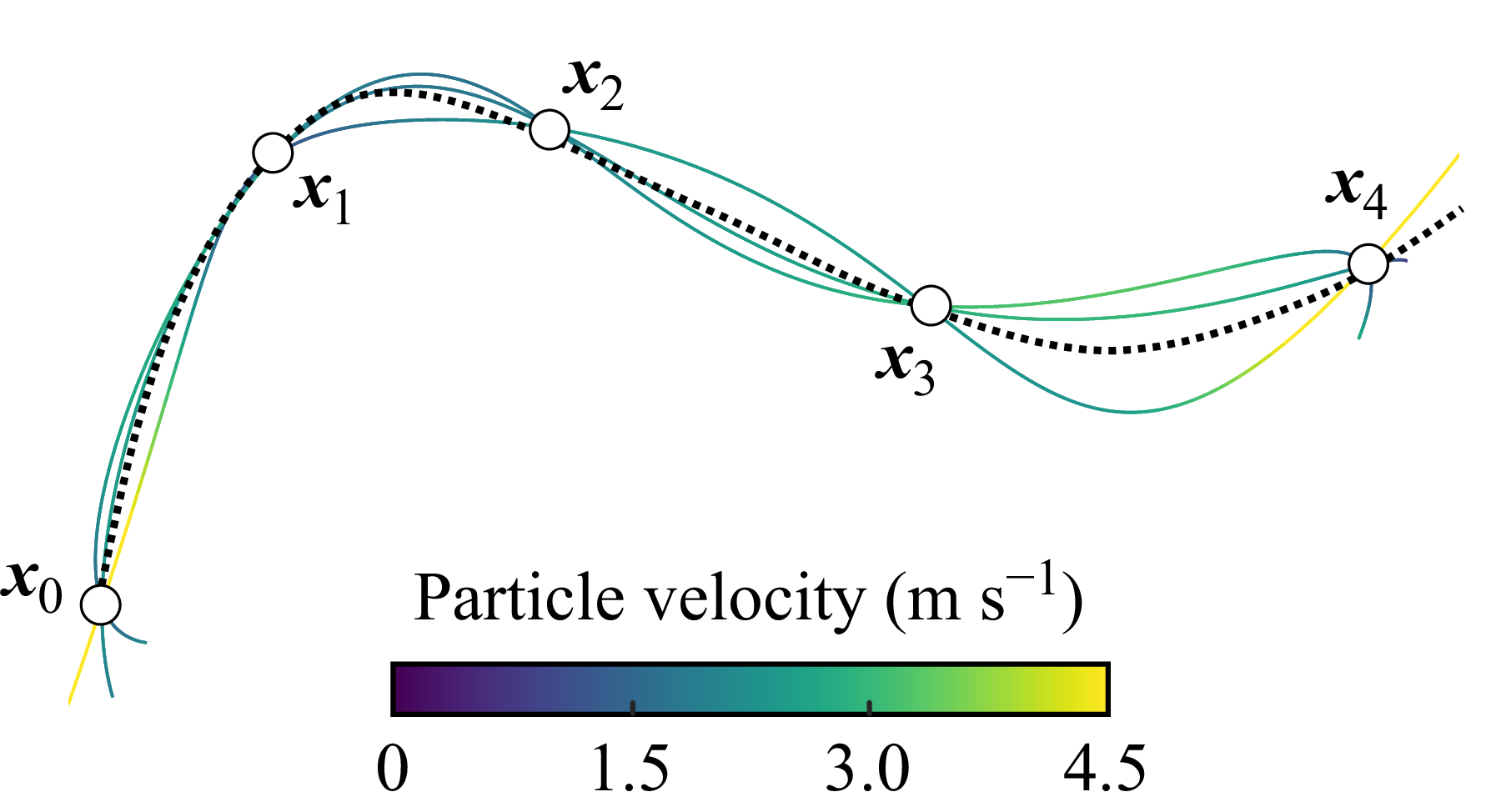
 θ
 θ

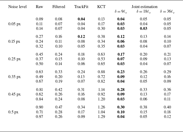
 x
 ℓν
 vν
 vν2/ℓν
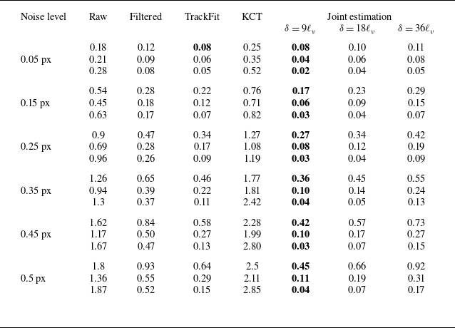
 z
 ℓν
 vν
 vν2/ℓν
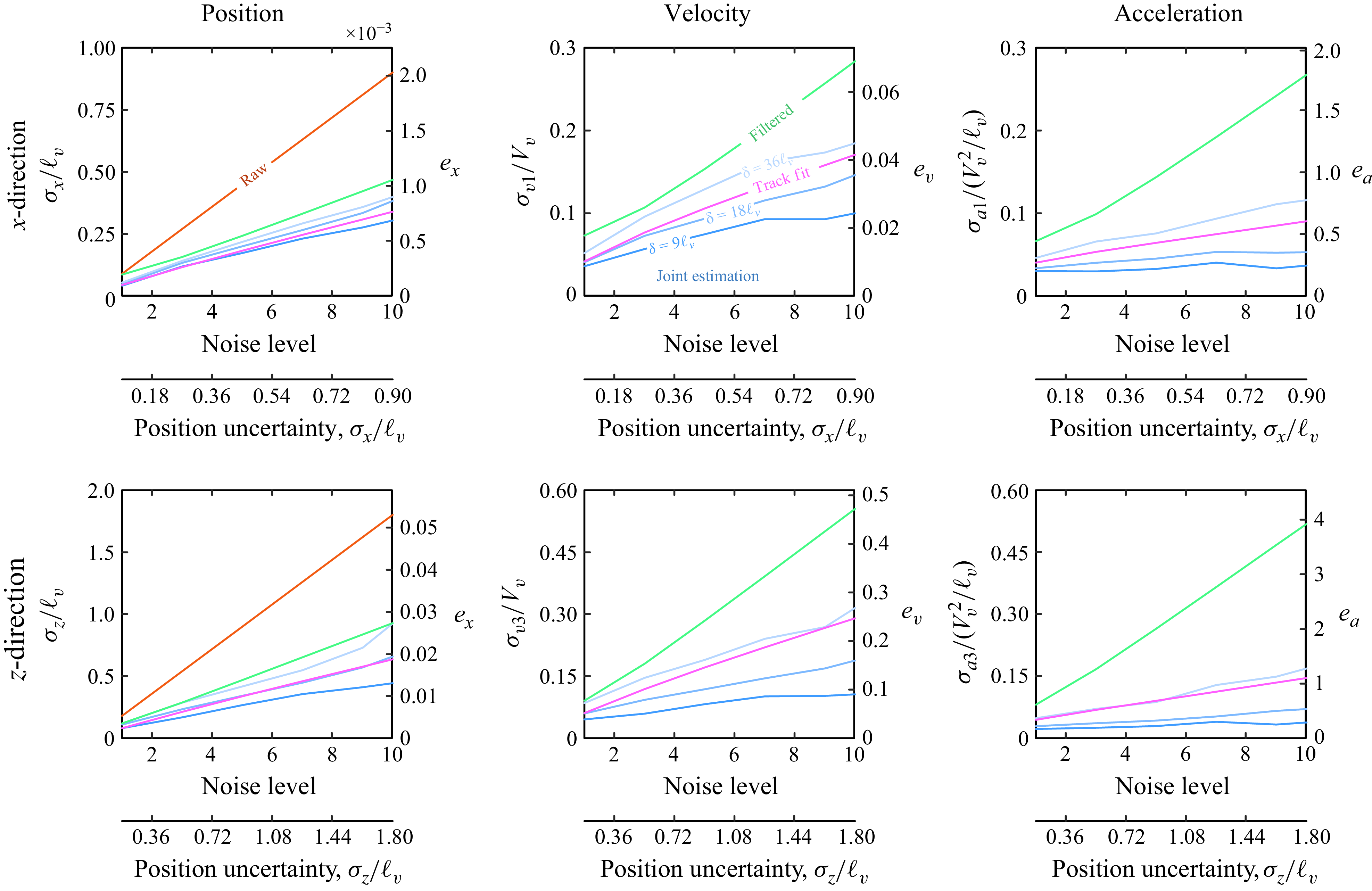
 x
 z
 δ=9ℓν
 18ℓν
 36ℓν
 δ=18ℓν
 36ℓν
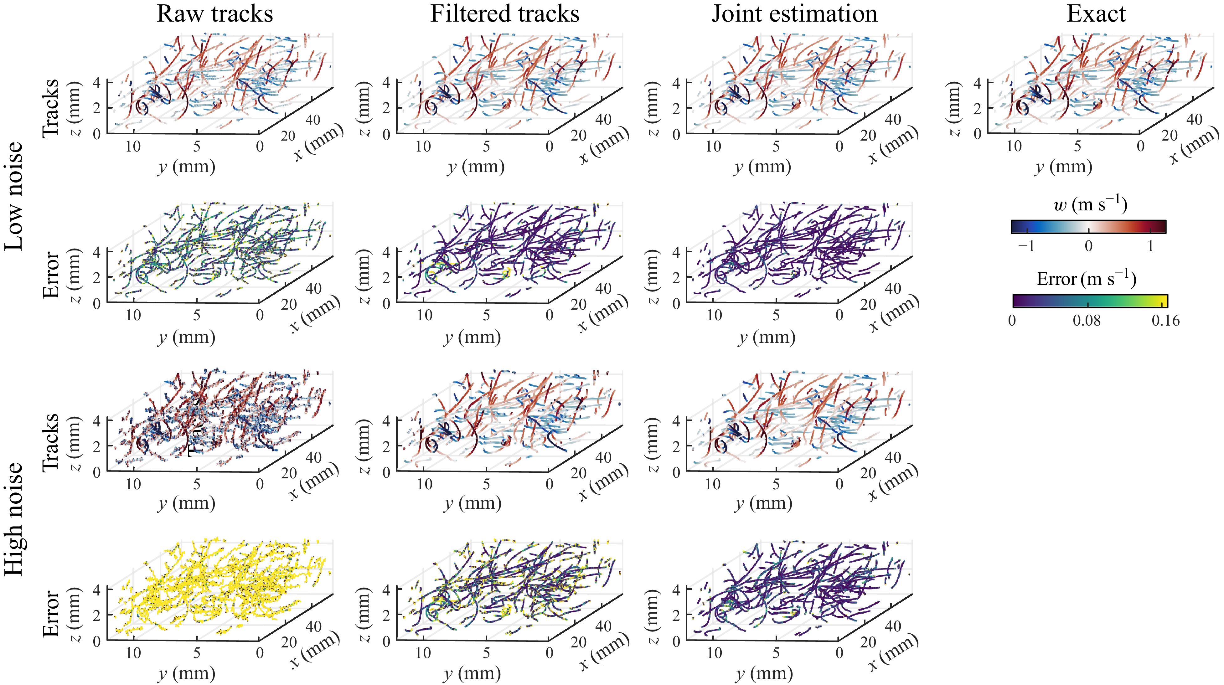
 σx=0.09ℓν
 σx=0.9ℓν
 δ=9ℓν
 v3
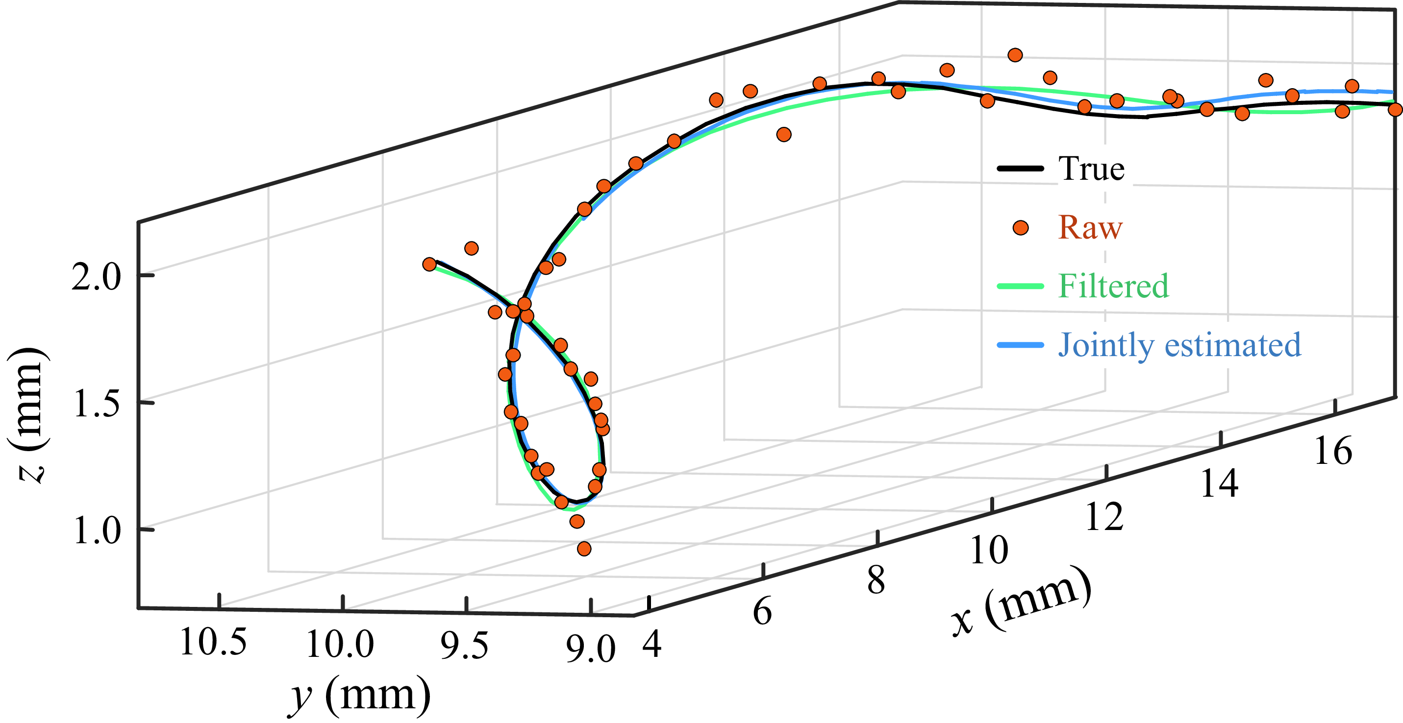

 σx=0.09ℓν
 δ=9ℓν
 −0.17
 u3
 p

 σx=0.9ℓν
 δ=9ℓν
 −0.17
 u3
 p

 σx=0.9ℓν
 δ=9ℓν
 Q
 Q=2.5×10⁶s−2

 9ℓν
 18ℓν
 36ℓν

 dp
 St

 −636.8
 −318.4
 u1
 u2
 −127.3
 u3
 −81.1
 p

 u=v
 St
 dp
 Q
 Q=5000s−2

 κNyq=1.007
 κNyq
 St
 St→0

 dp

 TiO2
 τp

 3

 dp
 ρp
 dp
 ρp
 dp


 dp
 dp

 dp

 St
 St→∞

 σx=0.3
 St
 St

 St
 St
 dp
 dp

 Rep
 Map
 Knp

 τp≈3
 3

 r=0.05
 0.1m

 τp≈3
 dp
 ρp

 1283
 2563
 5123
 1283
 2563
 5123

 St→0

 Open access

