1. Introduction
With the rapid development of various smart sensors, computer vision, pattern recognition and artificial intelligence technologies, vision-based target detection has become a hot topic in the field of intelligent vehicles and transport systems. In target detection, obstacle type recognition plays an important role in unmanned surface vehicle (USV) navigation, especially in cluttered environments (Mousazadeh et al., Reference Mousazadeh, Jafarbiglu, Abdolmaleki and Omrani2018; Polvara et al., Reference Polvara, Sharma, Wan, Manning and Sutton2018). The accurate recognition of obstacle type contributes to USV autonomous navigation operations, such as path planning (Long et al., Reference Long, Zuo, Su, Li and Zhang2020), obstacle avoidance (Shi et al., Reference Shi, Su, Wang, Wan and Luo2019) and reactive control (Wan et al., Reference Wan, Su, Zhang, Shi and AbouOmar2020).
For autonomous navigation of an unmanned vehicle, onboard visual camera and Laser Imaging Detection and Ranging (LIDAR) systems are normally utilised to capture images of the environment. Unlike LIDAR, a visual sensor is a visible light imaging device without movable parts, which makes it highly resistant to the mechanical stress encountered in USV operations. Although visual images are susceptible to weather conditions, the image characteristics of dynamic obstacles are richer than those obtained by LIDAR (Prasad et al., Reference Prasad, Rajan, Rachmawati, Rajabaly and Quek2017). In addition, the weight and size of the visual sensor is better for hull stability, and it does not interfere with other electronic devices (Bovcon et al., Reference Bovcon, Mandeljc, Perš and Kristan2018).
Currently, visual detection technologies are commonly installed on non-stationary buoys or ships for maritime environmental surveillance (Zhang et al., Reference Zhang, Li and Zang2017). However, obstacle type recognition for USV autonomous navigation based on visual images is still in the conventional computer vision stage. For instance, Hermann et al. (Reference Hermann, Galeazzi, Andersen and Blanke2015) utilised a camera system on a high-speed USV as an additional aiding sensor, mainly for horizon line detection, but obstacle type recognition has not been fully realised. For the detection or recognition of obstacles, the video sequences from visual systems are first transmitted to an image processing centre in real time. Then, the location and type of each obstacle is marked with a rectangular box on the image. The difficulties of obstacle type recognition include the following.
(1) Due to the phenomenon of mutual obstruction between obstacles such as ships, buoys, bridge piers, and other floating objects, obstacles often suddenly appear or disappear in dynamic scenarios.
(2) The presence of glinting/reflections on the water surface seriously interferes with the accuracy of obstacle recognition.
(3) The complexity of the shore background (buildings, ships at anchor, etc.) greatly affects the efficiency of obstacle recognition, but information about the shore background has no significance for USV autonomous navigation.
The above difficulties create certain challenges for obstacle type recognition for USV autonomous navigation. To remedy these limitations, a novel obstacle type recognition method is proposed for solving the above difficulties via a dilated convolutional neural network (CNN), which uses faster region-based convolutional neural network (R-CNN) and ResNet50 network. Some of the specific impacts that cluttered scenes have on obstacle detection need to be studied. Specific cluttered scenes may include the rolling and pitching of the USV, light changes, glare reflection, occlusion between obstacles, etc. Additionally, the various types of obstacles (cruise ships, barge ships, container ships, passenger ships, floating objects, speedboats, engineering ships, dredge ships, bridge piers and buoys) need to be distinguished. Obstacle type recognition lays the foundation for the intelligent identification and tracking of an obstacle.
The remaining content of this work is organised as follows. Section 2 provides a brief overview of target detection. The specific structure of the novel obstacle type recognition system is presented in Section 3. Section 4 designs an obstacle type recognition model using a dilated CNN. The experiments for verifying the proposed obstacle type recognition method are elaborated in Section 5. Section 6 and Section 7 wrap up the entire work with a related discussion and concluding remarks.
2. Related work
Few methods are available specifically for obstacle type recognition, but there are many methods for detection of ships. Considering that ships are the most critical target among many types of obstacles, this work expands further on ship detection methods. Therefore, the discussion of related work is focused on target (ship) detection methods and is divided into the following two subsections: conventional computer vision and deep learning techniques.
2.1 Conventional computer vision techniques
Target detection methods based on conventional computer vision techniques are generally divided into four categories. The first category is based on edge and contour features. For example, Hermann et al. (Reference Hermann, Galeazzi, Andersen and Blanke2015) and Fefilatyev et al. (Reference Fefilatyev, Goldgof, Shreve and Lembke2012) segment the obstacle ships from the target region under the estimated horizon by extracting the horizon using the operation of Canny edge extraction and Hough transform methods. Edge and contour features are widely applied in maritime target detection methods (Yan et al., Reference Yan, Chu, Xie and Yan2014). Although these methods have the characteristics of simplicity and small amounts of calculation, they may not perform well once targets are mixed with complex backgrounds.
The second category mainly uses the difference in various texture information from global features of visual images. Selvi et al. (Reference Selvi and Kumar2011) combined colour and texture components, and proposed a ship detection method via the local binary pattern. Loomans et al. (Reference Loomans, Peter and Wijnhoven2014) devised a robust target detector method based on the multi-scale histogram of gradients (HOG). Everingham et al. (Reference Everingham, Eslami, Gool, Williams, Winn and Zisserman2015) proposed a deformable part model based on the HOG, and achieved the best detection performance for 20 classes, including ships. Zhang et al. (Reference Zhang, Li and Zang2017) designed a ship detection algorithm based on the discrete cosine transform for maritime surveillance on non-stationary platforms. The above methods benefit from the texture consistency within sea-surface backgrounds but improve the recognition accuracy by relying greatly on texture information.
The third category relies on subtraction of background modelling. The specific methods include: modelling the median values of n video frames (Hu et al., Reference Hu, Yang and Huang2011) or adopting Gaussian functions to model the background and subtracting them (Frost and Tapamo, Reference Frost and Tapamo2013). Kristan et al. (Reference Kristan, Sulic, Kovacic and Perš2015) designed a graphical mask for obstacle detection via a semantic segmentation algorithm that generates a water segmentation mask and treats all objects outside of the water region as background. However, these methods require relatively stable background information, which is difficult to guarantee for a moving USV.
The fourth category imitates the mechanism of human visual attention. These methods utilise the high contrast of the target over the surrounding pixels. Liu et al. (Reference Liu, Zhou, Bai and Yu2012) realised the additional enhancement on visual attention model for ship target detection. Agrafiotis et al. (Reference Agrafiotis, Doulamis, Doulamis and Georgopoulos2014) combined the visual saliency map with Gaussian mixture model (GMM) to distinguish targets during maritime surveillance. Bovcon et al. (Reference Bovcon, Mandeljc, Perš and Kristan2018) designed a stereo obstacle detection method for the moving USV by combining hull roll and pitch measurements from the inertial measurement unit (IMU). Once the saliency of the obstacle is not obvious or the interference is at a higher order of magnitude, the obstacle recognition method based on the visual saliency map may become inaccurate.
2.2 Deep learning techniques
Deep learning techniques have achieved inspiring results in computer vision tasks over the past decade, such as face recognition, pedestrian recognition, and traffic signal recognition. Among these techniques, deep CNNs are commonly applied (Krizhevsky et al., Reference Krizhevsky, Sutskever and Hinton2012). In general, a CNN model usually includes two components: feature extraction and classification. The former is obtained through multi-layer stacks such as convolution, activation and pooling, while the latter outputs the score of each category through fully connected layers (Szegedy et al., Reference Szegedy, Liu, Jia, Sermanet, Reed, Anguelov, Erhan, Vanhoucke and Rabinovich2014). The CNN models commonly used for target detection mainly include AlexNet, ZF, GoogLeNet, VGG and ResNet (He et al., Reference He, Zhang, Ren and Sun2016).
The mate-architectures of target detection networks for CNN model training can be divided into region proposal-based and regression-based training. The former is two-stage training represented by R-CNN, fast R-CNN, and faster R-CNN (He et al., Reference He, Zhang, Ren and Sun2016). Regression-based training is single-stage training represented by a single shot multi-box detector and ‘you only look once’ (YOLO). Compared with single-stage training networks, two-state training networks generally have higher average precision but lower detection efficiency.
In addition to these conventional methods, scholars have increasingly begun to explore whether a machine can autonomously recognise an obstacle by deep learning, instead of utilising manually designed features, as in Kaushal et al. (Reference Kaushal, Khehra and Sharma2018). To cope with challenges such as motion blurring, scale changes, poor lighting conditions, background clutter and obstacles occluding each other, deep learning techniques are applied to identify images automatically (Nguyen et al., Reference Nguyen, Nguyen, Tran, Sang and Jeon2017). Deep learning is capable of extracting image features automatically and without spending additional effort in image preprocessing, which can significantly improve accuracy and efficiency. For instance, Zou and Shi (Reference Zou and Shi2016) and Zhang et al. (Reference Zhang, Jian, Zhang, Chen and Zhang2016) proposed singular value decomposition (SVD) networks and ship-CNN, respectively, for learning features from remote sensing images. Dairi et al. (Reference Dairi, Harrou, Senouci and Ying2018) utilised deep learning-based stereovision for unsupervised obstacle detection in driving environments. Meng et al. (Reference Meng, Hirayama and Oyanagi2018) developed an underwater drone for automatic fish recognition based on deep learning, which realised a detection system operating in real time and with high accuracy. Chen et al. (Reference Chen, Yang, Wang, Wu, Tang, Zhao and Wang2020) proposed a coarse-to-fine cascaded CNN for ship type recognition. Learned features based on deep learning provided substantial improvements in target detection as well as references for obstacle type recognition in USV autonomous navigation.
In this study, the obstacle type recognition system is implemented as the basic guarantee for obstacle avoidance in USV autonomous navigation. Higher priority is given to the system's average precision than its detection speed. Therefore, faster R-CNN is chosen for the original backbone architecture, while ResNet50 is chosen for the main feature extraction network. At the same time, a dilated convolution module is added to increase the field of view perception and improve the network's ability to learn the obstacle features in an image. The proposed network not only solves the problem of slow speed caused by selective search algorithms but also solves the bottleneck of slow detection of significant targets by sharing the previous convolution calculation.
3. Proposed autonomous recognition of obstacle type in visual images
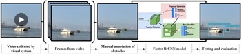
As the key link in USV navigation in this study, the autonomous recognition of obstacle type in visual images relies on the deep learning model. The block diagram in Figure 1 shows that the proposed system for autonomous obstacle type recognition in visual images using the dilated CNN includes: (1) video capture by the visual system, (2) extraction of frame images from the video, (3) annotation of manual obstacles, (4) model design and training, and (5) testing and evaluation. The specific details of the USV's visual sensor, image collection, model design and training, testing and evaluation parameters are presented in the following subsections.
Schematic of the autonomous obstacle type recognition system

3.1 Overview of the USV's visual sensor
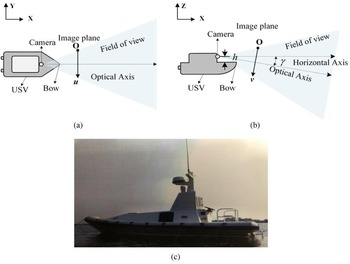
An USV is mainly driven forward during a voyage and rarely driven in reverse. Therefore, the videos obtained from the forward-looking visual sensor are referred to as the input frame images. The positional relationship between the camera and USV deck, as shown in Figures 2(a) and 2(b), and the shape of the test USV is shown in Figure 2(c). Among them, h and $\mathrm{\gamma }$ represent the height of camera from the deck and the angle between the optical axis and horizontal axis, respectively. These two parameters have an important influence on the field of view of the captured video.
Camera setup (a) top view, (b) side view, and (c) test USV

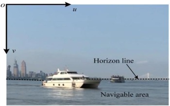
This study uses an Ezviz® Solo autonomous camera with a resolution of $1920 \times 1080$ pixels to collect and record video at 25 frames per second (FPS). The captured frame is shown in Figure 3, where the coordinate system is expressed as $({\textrm{u},\textrm{v}} )$
 in pixels with the origin point located at the top left. The frame is divided by the horizon line into two parts: the background area and the water surface. The water surface is also called the navigable area, and obstacle detection is focused on this area. The parameters h and $\mathrm{\gamma }$
 affect the proportion of the navigable area in the entire image.
Frame image captured by the test USV

3.2 Image collection
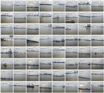
The authors collected $64$ video sequences of variable length at a resolution of $1920 \times 1080$
 pixels. A random frame from the $64$
 sequences is shown in Figure 4. Of the 64 sequences, $57$
 contain at least one type of obstacle. At least $16$
 sequences were captured in a cluttered environment, where the resulting disturbances make it difficult to detect and recognise obstacles. For example, Sequence28 and Sequence55 are tilted images resulting from significant rolling and pitching of the USV; Sequence1, Sequence5, and Sequence57 show the phenomenon of fogging on the water surface; Sequence3, Sequence43, Sequence48, Sequence60 and Sequence63 show sun glinting and reflection on the water.
Random frames from $64$ video sequences

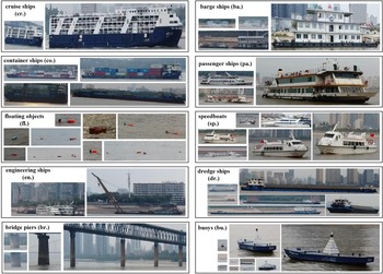
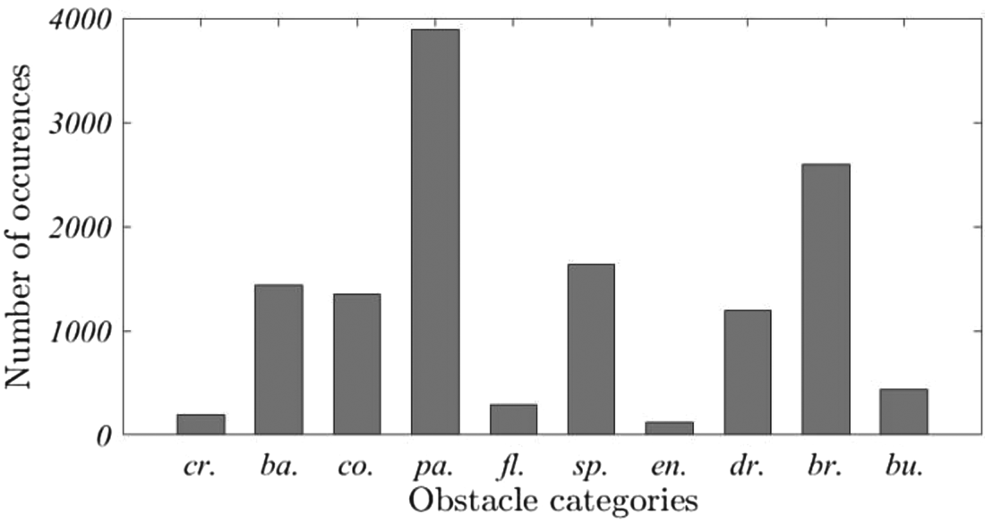
As the difference between adjacent frames is small, it is necessary to down-sample the video stream, that is, to store five frames per second as the sample for image annotation. After subtracting frames that do not contain any obstacles, the dataset contains a total of 8,040 frames, which contain 10 categories of obstacles: cruise ships, barge ships, container ships, passenger ships, floating object, speedboats, engineering ships, dredge ships, bridge piers and buoys. Some samples of the collected obstacle images are shown in Figure 5. The distribution of the obstacle occurrences is shown in Figure 6. To save space in the picture, abbreviations are used, e.g., the abbreviation ‘$\textrm{cr}.$ ’ stands for ‘cruise ship’ (and likewise for the other abbreviations).
Examples of each obstacle type

Distribution of obstacle categories

3.3 Dataset production
The accuracy of the recognition system is affected by the weather, lighting conditions, camera installation, and the categories and locations of obstacles. According to the different scenes, the testing dataset is divided into two groups: Group A collected under a normal environment and Group B collected under a cluttered environment. Meanwhile, the same number of frames in Group B are randomly selected from Group A to form Group C, which performs image augmentation by flipping, scaling and rotating. Group D contains all the mixed frames of Group A, Group B and Group C. The differences between the datasets of the four groups were shown in Table 1.
Specific differences of the four datasets

Generally, normal scenes specifically refer to the frames that are without obvious interference and relatively clear. Cluttered scenes mainly include the following situations: poor lighting conditions, interference caused by light reflection, water surface fogging, obscured obstacles, and the tilting of the image caused by significant rolling and pitching of the USV.
4. Applied recognition model based on the dilated convolutional operator
4.1 Dilated convolutional operator
The dilated convolution operator was initially applied to wavelet decomposition, and later extended to target detection, image segmentation and other fields (Yu and Koltun, Reference Yu and Koltun2016; Li et al., Reference Li, Zhao and Zhang2019; Xu et al., Reference Xu, Cao, Udupa, Tong and Torigian2020). The dilated convolution achieves the purpose of increasing the receptive field by inserting zero values into the convolution kernel.
Suppose that the discrete function $F:{{\mathbb{Z}}^2} \to {\mathbb{R}}$ , ${{\Omega }_r} = {[{ - r,r} ]^2} \cap {{\mathbb{Z}}^2}$
 , and define the discrete filter $w$
 : ${\mathrm{\Omega }_r} \to \mathrm{\mathbb{R}}$
 , the size of $({2r + 1} )\ast ({2r + 1} )$
 . The dilated convolutional operator ${ \otimes _\alpha }$
 can then be described as:

where $\mathrm{\alpha }$ indicates the order of dilated convolution, while $\mathrm{\alpha } = 1$
 means the dilated convolution operator degenerates to the convolution operator. For an ordinary convolutional operator with a kernel size of $k\ast k$
 , the range of affect is calculated as:

where ${H_i}$ and ${H_o}$
 denote the input feature map and output feature map, respectively. $\textrm{Pad}$
 means zero padding, $Str$
 is the sliding step, and $\textrm{floor}({\cdot} )$
 is the downward rounding function. The affect range of $\alpha$
 -dilated convolution is calculated as:

Define the $\alpha$ -dilated convolution$\; (\alpha > 1)$
 , thus $H_o^\alpha > {H_o}$
 . Compared with other mainstream approaches to feature extraction using an ordinary CNN, an $\alpha$
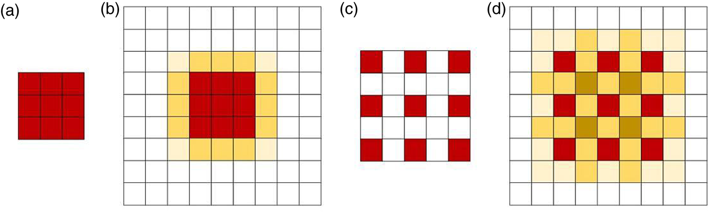
 -dilated convolutional operator allows the network to expand the receptive field domain without increasing the computational load of the calculation. Figure 7 illustrates the convolutional operator and the dilated convolutional operator, respectively.
Illustration of convolutional operator and dilated convolutional operator. (a) represents the convolution kernel size: $k = 3\mathrm{\ast }3$ ; (b) represents the response result of the centre pixel of a $9\mathrm{\ast }9$
 image after the convolution process. When the kernel is directly performed on the red area, the convolution affects the pixel range (considering the continuity of the image, there is a correlation between adjacent pixels and pixels) in a $5\mathrm{\ast }5$
 yellow area; (c) represents a $3\mathrm{\ast }3$
 convolution kernel with two dilated convolutional, and its receptive field increases to $5\mathrm{\ast }5$
 ; (d) indicates that the dilated convolutional operator affects the pixel range in a $7\mathrm{\ast }7$
 yellow area, and the calculation is not increased. The shade of yellow indicates the magnitude of the affect

Figure 7 fully demonstrates the role of dilated convolution in expanding the receptive field domain. When each pixel is operated on by dilated convolution, the response intensity of the feature map can be greatly improved. The feature extraction operation can be better completed, and a more accurate feature map of the input image can be obtained. The applied recognition model introduces a dilation rate to define the spacing of the data values processed by the convolution kernel during the convolutional layer. The convolutional operation mainly obtains the feature map through downsampling, such as the maximum value pooling method, which makes the size of the feature map obtained by sampling smaller and smaller. The original input image corresponding to each pixel on the obtained feature map covers a large area, which may result in sparse features. To avoid the phenomenon of sparse features, a dilated convolutional operator is applied to the convolutional layer.
4.2 Model design and optimisation
Analysis of the images collected by the USV visual sensor reveals that the characteristics of the same obstacle are quite different under different navigation conditions. For example, the scale of an obstacle will appear different based on its distance from the USV, and its colour will also change with the lighting conditions. If the receptive field can be increased through a dilated convolution operator, the obstacle information in the feature map can be enriched to a certain extent, which can further promote the network's ability to recognise various obstacle types in a cluttered environment. Therefore, this paper proposes an obstacle type recognition model based on a dilated CNN that applies faster R-CNN as the main architecture, including a backbone network based on ResNet50, deep-level feature extraction operations through dilated convolution, and the classification and regression region proposal network (RPN).
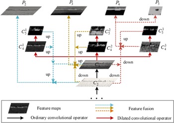
The specific application combines the dilated convolution with the ResNet50 network by replacing the ordinary convolution in the deep-level features $\{{{C_4},{C_5}} \}$ extracted by ResNet50 with the dilated convolution. As shown in Figure 8, the backbone network is optimised by the dilated convolutional operator. More specifically low-dimensional features contain a large number of trivial features, e.g., contours, textures and corners. However, there are distinctive features that can be used as a core component to distinguish similar targets. As the dilated convolution does not need to increase the parameters of the network, the detection is more convenient and faster, which improves the speed and efficiency of obstacle type recognition.
Backbone network optimised by the dilated convolutional operator

After the feature map of dilated convolution, a RPN is added to generate an object proposal region. For example, a small sliding window (size:$3 \times 3$ ) is proposed to slide over the lower-dimensional feature map, and projected to a lower n dimensional feature through the intermediate layer. For each sliding window location, nine anchor boxes are generated, which are determined by the number of aspect ratios and scales used in this model. There are three scales with box areas of ${128^2}$
 , ${256^2}$
 and ${512^2}$
 pixels, and three aspect ratios of $1:1$
 , $1:2$
 , and $2:1$
 , leading to nine region proposals. The extracted features are fed into fully connected layers, namely, the bounding box regression layer and classification layer, respectively. Meanwhile, non-maximum suppression is applied to reduce the overlapping regions by merging proposals that have high intersection of union.
The loss function of the RPN in faster R-CNN was calculated by He et al. (Reference He, Zhang, Ren and Sun2016):

where i indicates the anchor number, and ${p_i}$ represents the predicted probability of anchor i being an obstacle. $p_i^\ast$
 indicates the ground truth label, where $p_i^\ast$
 equal to one means it is positive, and zero means negative. ${N_{cls}}$
 and ${N_{reg}}$
 are normalisation components and are weighted by a balancing weight $\lambda$
 . The classification loss ${L_{cls}}$
 and the regression loss ${L_{reg}}\;$
 are given as follows:


where ${R_{{L_1}}}$ is the robust regression loss function, ${t_i}$
 is a vector representing the coordinates, and $t_i^\ast$
 indicates the ground truth coordinates. The parameterisations of the four coordinates are calculated as follows:


where x, y, w and h denote the centre coordinates, width and height, respectively. x, ${x_a}$ and ${x^\ast }$
 represent the corresponding values of the predicted and ground truth, as do variables y, w and h.
4.3 Model training
In this study, the technique of transfer learning is utilised to train the applied obstacle type recognition model, that is, the network parameters are initialised using the model parameters pre-trained in other large datasets, and then the dataset is used to fine-tune the parameters. The faster R-CNN and ResNet50 used in this study were initialised by the model parameters pre-trained in ImageNet. The training steps are as follows:
(1) Prepare the training and testing dataset and manually mark the collected training samples with the ground truth label;
(2) Initialise the RPN network parameters with the dilated CNN, and fine-tune the RPN network using a backpropagation algorithm and a random gradient descent algorithm;
(3) Initialise the fast R-CNN parameters with the dilated CNN, and extract the proposal regions using the RPN network by step (2) to train the obstacle type recognition network;
(4) Reset the RPN network parameters with the trained obstacle type recognition network, and fine-tune that part of the RPN network separately;
(5) Extract the proposal regions by using the fine-tuned RPN network in step (4) to fine-tune the obstacle type recognition network;
(6) Repeat steps (4) and (5) until the network converges or reaches the set maximum number of training sessions and the training process ends.
4.4 Model evaluation
The obstacle type recognition model is evaluated by the precision-recall curve, average precision, mean average precision, missing rate and detection speed.
(1) Precision-recall curve: Precision and recall as two conventional evaluation metrics can be calculated using:
(10)\begin{align}\textrm{precision} & = \frac{{\textrm{TP}}}{{\textrm{TP} + \textrm{FP}}}\end{align} (11)\begin{align}\textrm{recall} & = \frac{{\textrm{TP}}}{{\textrm{TP} + \textrm{FN}}}\end{align}


where $\textrm{TP}$ , or true positive, means the number of ground truth (GT) obstacles that are correctly detected. $\textrm{FP}$
 is false positive, which means that non-obstacles (background) are predicted as obstacles. $\textrm{FN}$
 is false negative, which means that GT obstacles are ignored, i.e., these obstacle are missing. A higher precision value reveals a high recognition accuracy, while a higher recall value indicates that almost no obstacles were missed. The precision-recall curve is composed of the recall value as the X-axis point and precision value as the Y-axis. The area under the precision-recall curve (AUC) reflects the accuracy of the obstacle type recognition model, that is, a larger area covered by the curve means a higher accuracy.
(2) $\textrm{AP}$
: The value of $\textrm{AP}$ denotes the average precision for the obstacle type recognition model as follows:
(12)\begin{equation}\textrm{mAP} = \frac{1}{{{N_{cls}}}}\mathop \sum \limits_i \textrm{A}{\textrm{P}_i}\end{equation}


among them, $p({\tilde{r}} )$ is the measured precision at recall $\tilde{r}$
 . The $\textrm{AP}$
 summarises the shape of the precision-recall curve, and is defined as the AP at a set of 11 equally spaced recall levels $\{{0,\;0 \cdot 1,\;0 \cdot 2, \ldots, 1} \}$
 .
(3) $\textrm{mAP}$
: The value $\textrm{mAP}$ is the mean AP for all classes and is calculated by:
(13)\begin{equation}\textrm{mAP} = \frac{1}{{{N_{cls}}}}\mathop \sum \limits_i \textrm{A}{\textrm{P}_i}\end{equation}
(4) $\textrm{MR}$
: The value of $\textrm{MR}$ represents the missing rate of the obstacle type recognition model, and is calculated as follows:
(14)\begin{equation}\textrm{MR} = \frac{{\textrm{FN}}}{{\textrm{TP} + \textrm{FN}}}\end{equation}


The value of $\textrm{MR}$ indicates the proportion of missed obstacles in the number of GT obstacles during the recognition process, that is, a lower value of $\textrm{MR}$
 means fewer obstacles are missed.
(5) $\textrm{FPS}$
: The value of $\textrm{FPS}$ is a typical indicator that is utilised to measure the detection speed of the deep learning model. The value of $\textrm{FPS}$ reflects the time required by the model to recognise the obstacle type in each frame. $\textrm{FPS}$ is the number of frames processed in 1 s.


5. Experiments and results
Three expreriments are conducted to investigate the proposed method. The obstacle type recognition system is implemented in a Pytorch platform, which provides libraries to build the architecture of deep learning models. The experiments are conducted on an Ubuntu 16⋅04 system with an Intel Core i7-8700 K CPU @ 3⋅70GHz${\times}$ 12 and NVIDIA GeForce GTX1080Ti GPU with 32G RAM. Experiment implementation details and the results are explained in the following sections.
5.1 Experiment 1 and results
The purpose of experiment 1 is to compare the deep learning method with the conventional computer vision method. The deep learning method uses a dilated CNN, while the conventional computer vision method is based on the Gaussian hybrid background model. The Gaussian hybrid based background modelling method can only determine the presence of an obstacle, but cannot identify the specific type of obstacle. For this reason, the block connected domain segmented using Gaussian hybrid based background modelling is considered as an obstacle. And it is considered as correctly detected if its overlap with the area covered by the GT box reaches 60% or more, otherwise it is considered as a missed detection. Similarly, the prediction box by the deep learning method is regarded as correctly detected if it overlaps with the GT box by more than 60%, without considering the specific type of classification. The recognition results of the two methods for Groups A and B are shown in Table 2.
Recognition results of traditional and deep learning methods

From Table 2, it can be seen that both the value of $\textrm{MR}$ and $\textrm{precision}$
 using the deep learning method are better than the Gaussian mixture background modelling method. For the Group A dataset under the normal scenes, the performance difference between the two methods is slightly smaller because there is no significant interference between the background and the obstacle in the normal scenes. The main performance difference between the two methods is reflected in the Group B dataset. The obstacle MR value of the background modelling method is close to 50%, and the $\textrm{precision}$
 value is less than 40%. This means that once the USV encounters a complex environment, it will result in most of the obstacles not being detected and recognised during autonomous navigation. Unlike the Gaussian hybrid based background modelling, the difference in recognition effectiveness between the two datasets resulting from the deep learning method is not significant. This is because the proposed obstacle detection and recognition method is based on a deep CNN network with constant translation, scaling and tilting, making it effective in overcoming the problems caused by mutual obstacle occlusion, scale change and screen tilt.
5.2 Experiment 2 and results
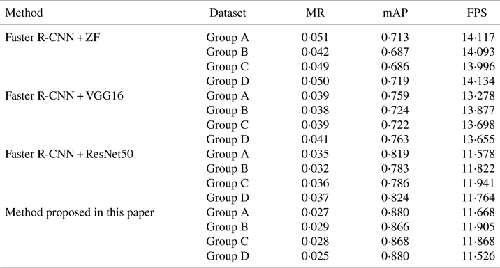
As the purpose of experiment 2 is to study the influence of the feature extractor and the size of the datasets on obstacle recognition effectiveness, the following subsections describe four datasets respectively tested by several deep learning networks that are fine-tuned for obstacle type recognition. In this work, faster R-CNN is investigated and applied with three convolutional feature extractors (ZF, VGG16, ResNet50). The proposed method combines the dilated convolution with the ResNet50 network as the feature extractor, which expands the receptive field domain to obtain high-level features. Detailed results using different methods and datasets are presented in Table 3 along with the value of $\textrm{MR}$ , $\textrm{mAP}$
 and FPS for each model.
The results using different methods and datasets

Table 3 confirms that the proposed method obtains better recognition accuracy than the other obstacle type recognition models. The results show that several CNN models recognise all of the various types of obstacles. Their missed rate is basically controlled within $6\%$ , and the mean recognition accuracy rate is mostly above $68\%$
 , which shows that the effect of using the deep learning techniques to recognise the obstacle type is quite satisfactory.
With respect to the $\textrm{AP}$ values of each class, Group D has the highest value of $\textrm{mAP}$
 and the lowest $\textrm{MR}$
 in all tests, and the recognition accuracy increases as the size of the datasets increases. Group A represents normal scenes, and its accuracy is better than that of Group B, which represents cluttered scenes. Cluttered scenes have less influence on the accuracy of the proposed model, which can be proved by the similar $\textrm{mAP}$
 and $\textrm{MR}$
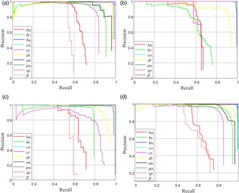
 values of Group B and Group C. The recognition accuracy of the model is positively correlated with the dataset size when the feature extraction master network is constant. It can be seen that the performance difference of the deep learning-based methods is not significant between normal sight scenes and cluttered scenes with comparable dataset sizes. This implies that dataset size has a positive effect on the recognition performance, because the more images are trained and tested, the more it helps the deep learning model to obtain richer feature information. The precision-recall curve for the 10 classes of obstacles using the four datasets are computed as shown in Figure 9.
Precision-recall curve for each class using different datasets. (a) Group A, (b) Group B, (c) Group C, (d) Group D

5.3 Experiment 3 and results
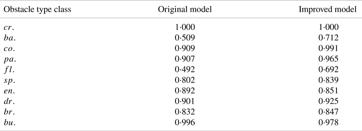
The purpose of experiment 3 is to compare the performance differences of the improved dilated CNN models on small-scale obstacle recognition. In this work, the Resnet50 network is improved by combining it with the dilated convolutional operator. The $\textrm{AP}$ values of the models before and after improvement for 10 categories of obstacles are shown in Table 4.
Specific AP values of Group D

The results in Table 4 show that the recognition effectiveness of the original model for two types of obstacles, namely, barge ships and floating objects, is much lower than the average. Because barge ships and floating objects are small and inconspicuous in the frames, both belong to the class of small-scale obstacle targets compared with large-scale obstacles such as cruise ships, container ships and passenger ships. The small-scale obstacle is easily lost in the deep feature map pooling, and this paper adopts multi-scale dilated convolutional operator to improve this phenomenon. The average accuracy is improved from 82⋅4% to 88%, mainly improving the recognition accuracy of two types of obstacles, the barge ships and floating objects.
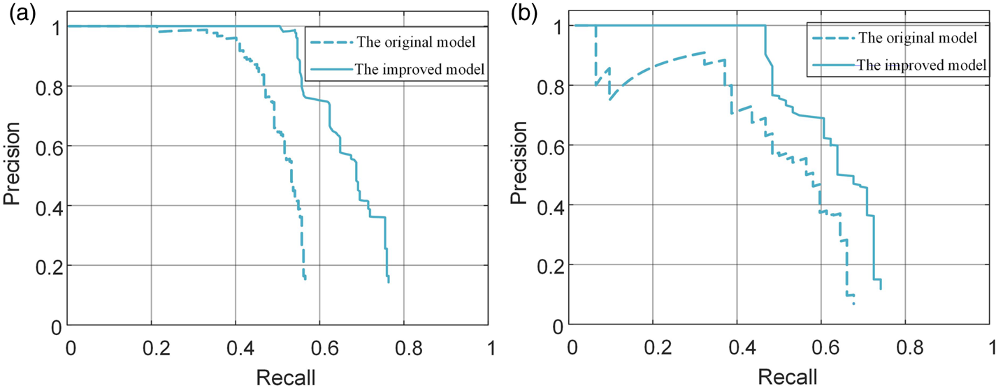
Figure 10 shows the performance improvement of the precision-recall curves for two small-scale obstacles, barge ships ($ba.$ ) and floating objects ($fl.$
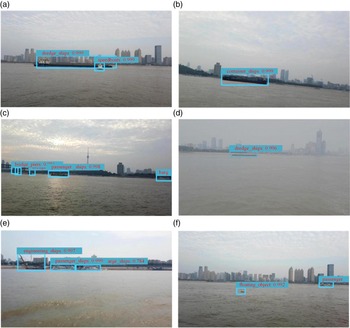
 ). And it can be seen that the area covered under the improved curve is larger than the original model, which indicates that the proposed model has improved the effectiveness of detection and recognition for small-scale obstacles. Figure 11 shows six examples of detecting obstacles in cluttered scenes.
Results of the precision-recall curves. (a) barge ships (ba.), (b) floating objects (fl.)

Results of recognition of obstacle types: (a) obstacles obscured, (b) image tilting, (c) sun setting, (d) water surface fogging, (e) cluttered background, (f) very small obstacles

6. Discussion
The proposed obstacle type recognition model using a visual sensor has been verified for USV navigation. The experiments indicated that network type, dataset size and cluttered environment can influence the performance of obstacle type recognition. First, the general rule is that deeper network layers can contribute to obtaining more detailed features. However, a deeper and complex neural network always means that a larger number of parameters need to be constructed, and the corresponding computational cost also increases as the network depth increases, which is why very deep or complex networks may not always be the optimal choice when constructing an appropriate deep learning model. It is worth noting that the recognition accuracy of these CNN models gradually increases; however, as the recognition accuracy increases, the detection speed gradually decreases. Therefore, when designing the obstacle type recognition system for USV navigation, the trade-off between the recognition accuracy and speed should be considered.
In addition, it was found that as the size of the datasets increases, the performance of the obstacle type recognition model continues to improve during the experiment. However, the dataset used to train and test the model is small due to experimental environment and the cost constraints. In this work, the pre-trained model in ImageNet was applied as the feature extractor to the small dataset by combining with transfer learning technique. Currently a quite small dataset needs to be expanded to enrich the diversity and improve the quality of datasets, which helps to enhance the detailed features of obstacles.
Finally, a cluttered scene can influence the recognition result, as shown for the Group A and Group B datasets. After excluding the influence of the inconsistent scale of the test datasets of Group A and Group B, the test results for these groups show that the proposed model is less affected by cluttered scenes. This improvement occurs because the proposed obstacle type recognition utilises a multi-scale dilated convolutional operator. This increases the value of $\textrm{mAP}$ to $88\%$
 by improving small-scale obstacle recognition, but there are still exist some problems to be mentioned. For example, small obstacles such as tiny floating objects, distant ships and bridge piers have a high probability of being incorrectly identified or undetected during testing. The reason for this phenomenon may be due to the tiny size of these obstacles or their similarity in colour to the colour of the water or background. Therefore, after overcoming the influence of the shape, size and colour of the obstacles, the type recognition model has room for further improvement.
7. Conclusion
The extensive application of deep learning techniques in intelligent marine equipment has become a trend in recent years, especially in the field of USV autonomous navigation. The visual system is an economical and convenient way for a USV to perceive the surrounding environment. Unlike ordinary ships operated by humans, a USV cannot rely on manual experience to identify obstacles. Previous obstacle detection methods focused on feature extractor methods – such as threshold segmentation, the multi-scale HOG method and the saliency map with GMM – require substantial effort for feature extraction. This paper proposes a deep learning model for recognising obstacle types in frames automatically using a dilated CNN. The main contribution of this paper is a novel method for USV intelligent autonomous navigation that is immune to cluttered environments and can meet the practical requirements of an obstacle type recognition system. In addition, rather than classifying obstacles into ships and non-ship targets, the proposed method subdivides various types of obstacles, laying the foundation for intelligent obstacle identification and tracking. In follow-up work, the authors will further study and judge the intention of dynamic obstacles based on this research, and identify dynamic obstacles that pose a security threat to USVs.
Acknowledgments
The authors would like to acknowledge the support of the Natural Science Foundation of China under Grants (Nos.61876219 and Nos.6150314), the Fundamental Research Funds for the Central Universities (Nos.175111001, Nos.2017-YB-030, and Nos.2018IVB084) and the Ideological and Political Department Project of Hubei Provincial Department of Education (Nos.21Q210).