1 Introduction
Boundary layer transition is a relevant phenomenon in many aerodynamic and aero-thermodynamic problems and has been extensively investigated from the past century till recent times (Kachanov Reference Kachanov1994). Among the factors affecting the boundary layer transition process, surface roughness plays a key role. When a roughness element with sufficiently large height (
 $h$
) compared to the boundary layer thickness (
 ${\it\delta}$
) is immersed in a laminar boundary layer, it will produce a disturbance with the potential to accelerate the transition process. Surface roughness is typically categorized in three types based on shape and distribution: two-dimensional (e.g. steps, gaps and wires); three-dimensional isolated elements; distributed roughness. The role of both isolated and distributed three-dimensional roughness in the process of promoting boundary layer transition is far from being fully understood, especially in relation to the effect of spanwise varying disturbances (Ergin & White Reference Ergin and White2006). Nevertheless, the triggering effect of isolated three-dimensional roughness can be predicted by the flow properties at the top edge of element, defined as roughness-height based Reynolds number,
 $Re_{h}=u_{h}h/{\it\nu}$
(van Driest & McCauley Reference van Driest and McCauley1960; Tani Reference Tani1969). Unlike two-dimensional roughness, where the transition location moves upstream gradually with the increase of
 $Re_{h}$
(Dryden Reference Dryden1953), three-dimensional roughness elements induce an upstream shift more rapidly when
 $Re_{h}$
exceeds a critical value (
 $Re_{h,crit}$
). Whereas below
 $Re_{h,crit}$
there will be little effect on the transition (Smith & Clutter Reference Smith and Clutter1959; Tani Reference Tani1969).
In low-speed flows, the onset of hairpin-shaped vortices shedding behind isolated roughness element has been generally associated to the process of early boundary layer transition (Acarlar & Smith Reference Acarlar and Smith1987; Klebanoff, Cleveland & Tidstrom Reference Klebanoff, Cleveland and Tidstrom1992). Ergin & White (Reference Ergin and White2006) studied the boundary layer downstream of a spanwise array of cylindrical roughness elements at both subcritical and supercritical roughness-height based Reynolds number (
 $Re_{h}$
) using hot-wire anemometry. The measured streamwise velocity fluctuations in the roughness wake revealed the possible existence of hairpin vortices, which originate from the Kelvin–Helmholtz (K–H) instability. However, the studies that link the existence of hairpin vortices to K–H instability are based either on two-dimensional flow visualization or statistical analysis from point-wise measurements. An isolated roughness element introduces a system of streamwise vortices, which perturb the spanwise homogeneity of the boundary layer by inducing low- and high-speed streaks (Fransson et al.
Reference Fransson, Brandt, Talamelli and Cossu2004). Andersson, Berggren & Henningson (Reference Andersson, Berggren and Henningson1999) found that steady streamwise vortices, later develop into low- and high-speed streaks, producing the optimal disturbances, which undergo maximum spatial energy growth, in turn leading to bypass transition. The stability of the resulting shear flow along with the unsteady fluctuations present in the wake of the roughness element have motivated a study using direct numerical simulations (DNS) (Rizzetta & Visbal Reference Rizzetta and Visbal2007) corresponding to the experiment of Ergin & White (Reference Ergin and White2006). A good agreement between numerical and experimental results was reported and the relation between K–H instability and transition was addressed.
Despite the attention devoted to the topic, the role of K–H instability remains controversial. In a recent study, Loiseau et al. (Reference Loiseau, Robinet, Cherubini and Emmanuel2014) conducted a three-dimensional global stability analysis over a cylinder. They reported that both varicose and sinuous modes, which are related to K–H and streaky instability, respectively, sustain in the wake. Which mode of the two is dominant in the transition process highly depends on the aspect ratio of the cylinder. In the compressible flow regime Choudhari et al. (Reference Choudhari, Li, Wu, Chang, Edwards, Kegerise and King2010) and Kegerise et al. (Reference Kegerise, King, Owens, Choudhari, Norris, Li and Chang2012) studied the flow over a square in the supersonic boundary layer both numerically and experimentally, and found that counter-rotating vortex pairs in the wake of roughness induce low- and high-speed regions and streak instabilities. Compared to shear layer instability, which undergoes rapid decrease with the streamwise distance from the roughness, streak instability persists in the downstream region. At lower
 $Re_{h}$
, the latter dominates the process of transition with final breakdown to turbulence. Therefore, more detailed numerical or experimental evidence is necessary to characterize the three-dimensional nature of the flow behind isolated roughness.
In subsonic flows, transition can be artificially promoted by either a roughness element (Lin Reference Lin2002) or by the use of a zigzag trip (van Rooij & Timmer Reference van Rooij and Timmer2003) in order to increase near-wall momentum and delay unwanted flow separation. Elsinga & Westerweel (Reference Elsinga and Westerweel2012) conducted a quantitative study of boundary layer transition behind a zigzag trip using tomographic particle image velocimetry (tomographic PIV). In the separated shear layer behind the zig–zag trip, spanwise vortices were observed, which develop into hairpin-like vortical structures further downstream. They concluded that unsteadiness in the shear layer strongly contributes to the velocity fluctuations and transition in the downstream region.
In the supersonic flow regime, roughness elements are often employed for passive control of the boundary layer, acting as vortex generators, which transport higher momentum flow towards the near-wall region. According to the investigation performed by Anderson, Tinapple & Surber (Reference Anderson, Tinapple and Surber2006), the micro-ramp geometry offers the advantages of strongly minimizing the transformed shape factor
 $H_{tr}$
of the boundary layer (Fukuda, Hingst & Reshotko Reference Fukuda, Hingst and Reshotko1975) and structural ruggedness when compared to the micro-vane. As a result, the micro-ramp geometry has received most attention as a vortex generator and it has demonstrated effectiveness in reducing flow separation caused by shock wave boundary layer interaction (SWBLI) (Dolling Reference Dolling2001; Babinsky, Li & PittFord Reference Babinsky, Li and PittFord2009).
Recent investigations have dealt with the flow topology over a micro-ramp immersed in supersonic turbulent boundary layers. Babinsky et al. (Reference Babinsky, Li and PittFord2009) studied the effect of ramp height and described a baseline surface flow topology. The wake consists of multiple counter-rotating vortex pairs, including one dominant primary pair and several secondary pairs. The primary vortex pair ejects low momentum fluid away from the wall in the region around the symmetry plane and entrains high momentum fluid downwards from the sides. The existence of the counter-rotating vortex pair was further confirmed by experimental visualization (Herges et al. Reference Herges, Kroeker, Elliott and Dutton2010) and numerical simulation (Lee et al. Reference Lee, Goettke, Loth, Tinapple and Benek2010).
Blinde et al. (Reference Blinde, Humble, van Oudheusden and Scarano2009) investigated the instantaneous flow organization past an array of micro-ramps using stereo PIV along wall-parallel planes. The presence of instantaneous counter-rotating vortices at the side of each element wake was ascribed to the leg portion of hairpin vortices, which agrees with observations in low-speed flows (Acarlar & Smith Reference Acarlar and Smith1987; Klebanoff et al. Reference Klebanoff, Cleveland and Tidstrom1992). The LES study by Li & Liu (Reference Li and Liu2010) reports a train of vortex rings produced in the highly sheared region of the wake. This vortex ring is further explained as a product of K–H instability, with a highly intermittent nature (Lu, Pierce & Shih Reference Lu, Pierce and Shih2010; Wang et al. Reference Wang, Liu, Zhao, Fan and Wang2012). Sun et al. (Reference Sun, Schrijer, Scarano and van Oudheusden2012) experimentally visualized the full three-dimensional flow organization using tomographic PIV. The instantaneous flow organization shows the presence of a train of arc-shaped vortices at the edge of the wake due to the K–H instability. In the downstream wake region of the micro-ramp, the K–H instability at the upper shear layer further develops with the onset of vortex pairing (Sun et al. Reference Sun, Schrijer, Scarano and van Oudheusden2014b ). In a more recent numerical study, Sun et al. (Reference Sun, Scarano, van Oudheusden, Schrijer, Yan and Liu2014a ) also investigated the temporal evolution of the latter vortices, concluding that the onset of arc-like vortices pairing and connection at the bottom in the downstream region contributes to the distortion of the streamwise counter-rotating vortex pair.
The above survey indicates the interest in the effect of isolated micro-ramps within a turbulent incoming boundary layer, with the special application of micro-ramps for SWBLI control. The resulting flow behaviour downstream of the micro-ramp is therefore to be connected to the presence of the micro-ramp in combination with the incoming boundary layer turbulence which in turn affects the stability of the overall wake structure. This interaction partly masks the mechanism of the wake evolution and the onset of instability. In this respect, studies in the laminar regime potentially yield a clearer scenario of transition and the instability mechanisms behind a submerged isolated micro-ramp. Tirtey, Chazot & Walpot (Reference Tirtey, Chazot and Walpot2011) studied the transitional flow over a micro-ramp in the hypersonic flow regime both numerically and experimentally revealing the presence of two pairs of counter-rotating vortices. Furthermore, secondary vortex structures were observed at the outer side of the primary vortices. The fast spreading behaviour of the secondary vortex pair downstream was conjectured to indicate the onset of transition. Although compressibility will have a stabilizing effect and delay transition, many features are still similar to the transition process at low speed, thus considered relevant (Redford, Sandham & Roberts Reference Redford, Sandham and Roberts2010; Bernardini, Pirozzoli & Orlandi Reference Bernardini, Pirozzoli and Orlandi2012). For similar flow conditions, Choudhari, Li & Edwards (Reference Choudhari, Li and Edwards2009) found that the micro-ramp introduces spanwise alternated low- and high-speed streaks resulting in velocity inhomogeneity in both wall-normal and spanwise directions. Further stability analysis indicated that streaky instability, which relates to spanwise velocity gradients, plays a more relevant role in the context of boundary layer transition. However, no observation of the dynamical behaviour of the flow could be reported and the related transition mechanism remains to be investigated. Moreover, the aforementioned studies mostly focus on the near-wake region (within 20 micro-ramp heights), whereas the vortex evolution process leading to transition would require observations in the far wake, where the turbulent regime is established.
Although the flow downstream of a micro-ramp has been studied rather extensively in turbulent (compressible) boundary layers, to some surprise, the flow around a micro-ramp submerged in a laminar and incompressible boundary layer has not been reported in literature. This case, although simplistic, would represent the reference scenario for boundary layer transition induced by a micro-ramp to which further studies in the compressible or turbulent regime may refer. The main objective here is to identify early stages of transition by detecting the three-dimensional oscillations of the wake. For this aim, tomographic PIV (Elsinga et al. Reference Elsinga, Scarano, Wieneke and van Oudheusden2006) is employed.
The methodology of the current study is detailed in § 2, where the flow facility and the measurement conditions are discussed. The characteristics of undisturbed boundary layer are discussed in § 3. The mean flow organization (§§ 4.1 and 4.2) identifies the streamwise vortical structures and the induced spanwise and wall-normal velocity variation. The details of unsteady flow activity are inspected by instantaneous visualization in § 4.3, with the aid of the vortex detection
 ${\it\lambda}_{2}$
criterion (Jeong & Hussain Reference Jeong and Hussain1995). The statistical analysis of velocity field fluctuations and turbulence production are given in § 5, aiming at a quantitative characterization of the wake turbulent structure and yielding the edge of turbulent/non-turbulent interface along with its spreading angle.
2 Experimental set-up and measurement technique
2.1 Flow facility and micro-ramp configuration
Experiments were carried out in the low-speed open test section wind tunnel (W-tunnel) of the Aerodynamics Laboratories of the Aerospace Engineering Faculty at TU Delft. The W-tunnel operates at room temperature and pressure with a test section of
 $0.4\times 0.4~\text{m}^{2}$
following a contraction ratio of 9 : 1. The maximum operating velocity of the tunnel is
 $35~\text{m}~\text{s}^{-1}$
and the turbulence level in the free stream is below
 $0.5\,\%$
.
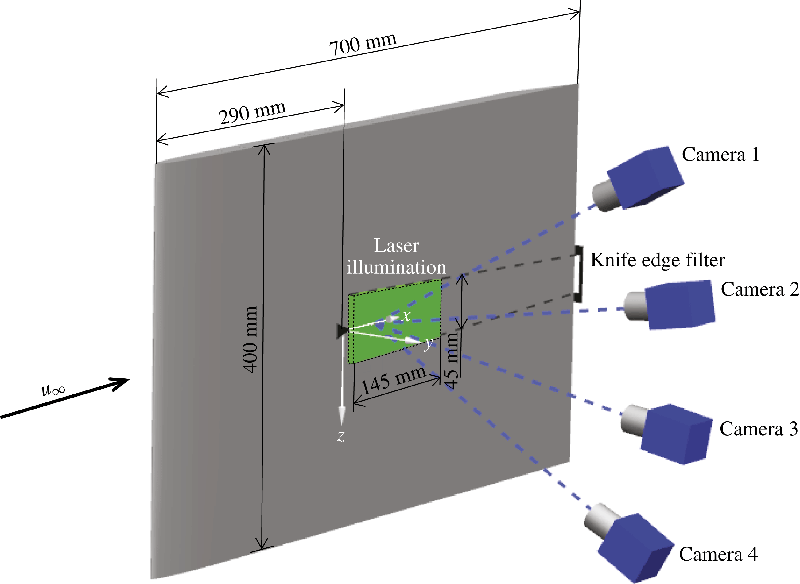
An aluminium flat plate of 700 mm long and 10 mm thick was installed in the mid-plane of the test section, spanning its entire width (400 mm). The plate was equipped with a modified super ellipse leading edge (Lin, Reed & Saric Reference Lin, Reed, Saric, Hussaini, Kumar and Streett1992), with no curvature discontinuity and preventing laminar flow separation. The plate terminates with a sharp trailing edge at a surface angle of
 $11.3^{\circ }$
with respect to the free-stream direction. The plate surface was covered by black matt adhesive foil to reduce laser refection during the tomographic PIV measurements. A micro-ramp, with a height (
 $h$
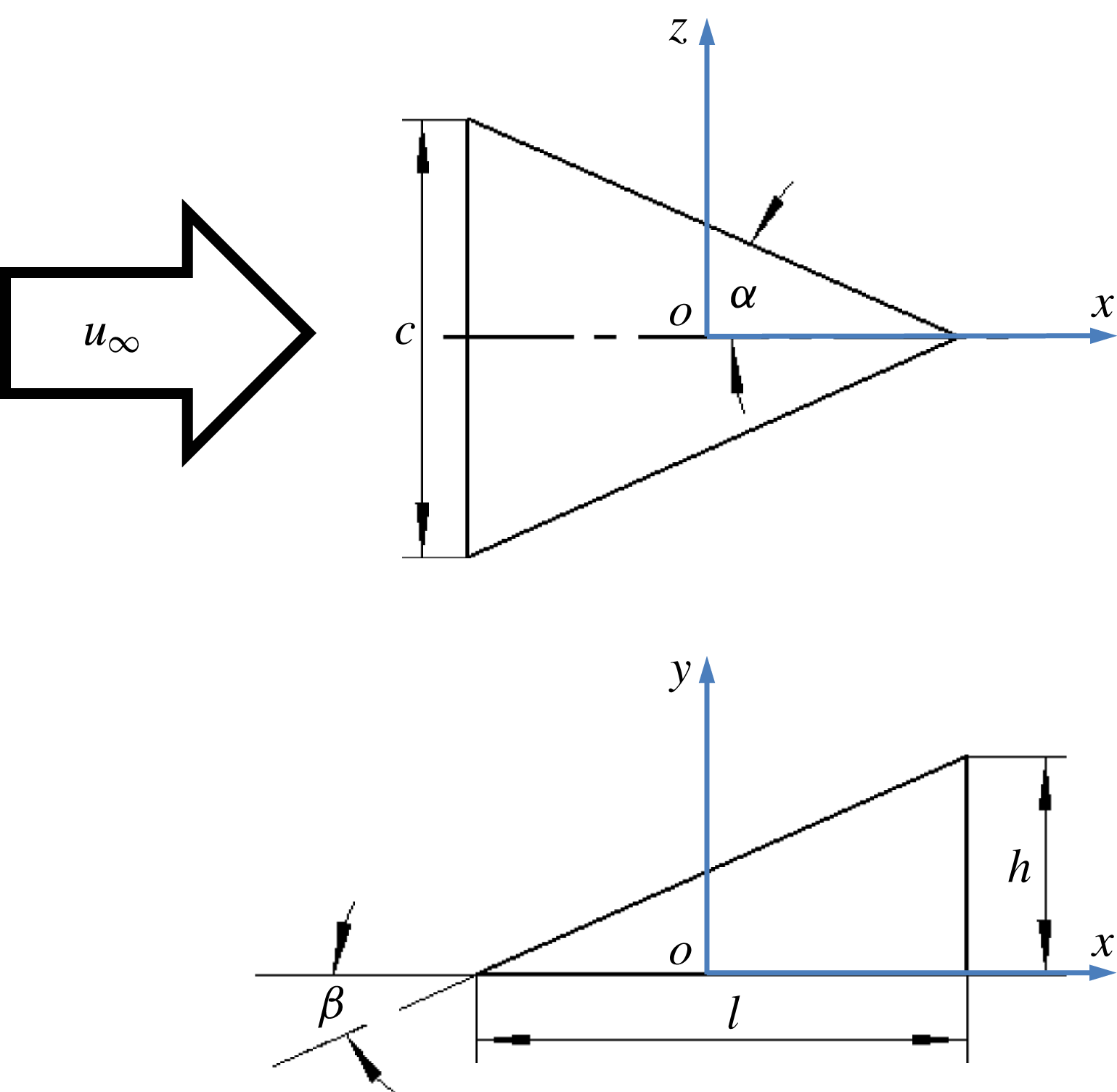
) of 2 mm, was installed on the plate at 290 mm downstream of the leading edge (figure 2). The micro-ramp has a chord length (
 $l$
) of 4.5 mm and a span width (
 $c$
) of 4 mm. The resulting half sweep angle (
 ${\it\alpha}$
) and incidence angle (
 ${\it\beta}$
) are both
 $24^{\circ }$
. The geometry of the micro-ramp follows the optimization study by Anderson et al. (Reference Anderson, Tinapple and Surber2006) and is one of the most reported in the literature (Babinsky et al.
Reference Babinsky, Li and PittFord2009; Herges et al.
Reference Herges, Kroeker, Elliott and Dutton2010; Sun et al.
Reference Sun, Schrijer, Scarano and van Oudheusden2012; Giepman, Schrijer & van Oudheusden Reference Giepman, Schrijer and van Oudheusden2014). Its schematic layout is illustrated in figure 1.
Micro-ramp geometry and definition of coordinate axes.

Experiments were conducted at a free-stream velocity of
 $10~\text{m}~\text{s}^{-1}$
. The corresponding Reynolds number based on micro-ramp height (
 $Re_{h}=u_{h}h/{\it\nu}$
) is 1170. Klebanoff, Schubauerand & Tidstrom (Reference Klebanoff, Schubauerand and Tidstrom1955) established that the critical Reynolds number
 $Re_{h,crit}$
for a roughness element with unity height-to-span ratio lies in the range between 600 and 900. For different values of the height-to-span ratio, the critical Reynolds number was found to scale with
 $(h/c)^{2/5}$
(von Doenhoff & Braslow Reference von Doenhoff, Braslow and Lachmann1961; Tani Reference Tani1969). Consequently, based on the micro-ramp
 $h/c$
value of 0.5, the current
 $Re_{h,crit}$
ranges from 455 to 682, indicating that the present experiments are conducted in the supercritical regime. At the micro-ramp position, the undisturbed laminar boundary layer thickness (
 ${\it\delta}_{99}$
) is 3.26 mm (
 $h/{\it\delta}=0.61$
). The measured shape factor is 2.59, indicating the laminar flow regime in the boundary layer. Relevant properties are summarized in table 1.
Schematic illustration of experimental configuration and tomographic PIV set-up.

Incoming flow conditions and boundary layer integral parameters.

2.2 Tomographic particle image velocimetry
Tomographic particle image velocimetry was adopted in the present investigation for its ability to describe the instantaneous three-dimensional distribution of velocity and vorticity.
The flow was seeded with a SAFEX fog generator. The working fluid is a water–glycol solution. The mean droplet size is
 $1~{\rm\mu}\text{s}$
and the particle concentration is approximately
 $4~\text{particles}~\text{mm}^{-3}$
. Pulsed illumination is obtained with a Quantel CFR PIV-200 Nd : YAG laser (
 $200~\text{mJ}~\text{pulse}^{-1}$
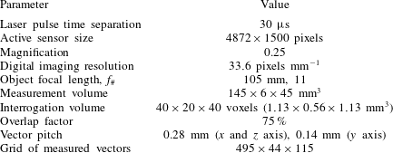
, 532 nm wavelength, 9 ns pulse duration) with pulse separation time of
 $30~{\rm\mu}\text{s}$
. An array of four LaVision Imager Pro LX interline CCD cameras (
 $4872\times 3248~\text{pixels}$
,
 $7.4~{\rm\mu}\text{m}~\text{pixel}^{-1}$
) was arranged subtending an arc to simultaneously record the images of the light scattered by the tracers in the illuminated region, as shown in figure 2. Although a linear arrangement of viewing directions yields lower reconstruction accuracy in comparison to a 2-D camera arrangement (Scarano Reference Scarano2013), the current choice of a planar angle of
 ${\it\beta}=60^{\circ }$
mitigates this disadvantage and returns a reconstruction quality comparable to that obtained subtending a solid angle. Each camera was equipped with an objective of 105 mm focal length mounted at an angle to comply with the Scheimpflug condition (Prasad & Jensen Reference Prasad and Jensen1995). The numerical aperture was set to
 $f_{\#}=11$
, resulting in a focal depth of 8.4 mm. The sensor was cropped in the vertical direction resulting in an active sensor region of
 $4872\times 1500~\text{pixels}$
. The corresponding measurement volume size is
 $145(x)\times 6(y)\times 45(z)~\text{mm}^{3}~(72.5h\times 3h\times 22.5h)$
. The resulting digital image resolution is
 $33.6~\text{pixels}~\text{mm}^{-1}$
corresponding to
 $35.4~\text{voxels}~\text{mm}^{-1}$
in the object space. The coordinate axes
 $x,y,z$
correspond to the streamwise, wall-normal and spanwise directions respectively. The origin is at the centre of the micro-ramp. The measurement domain extends from 5 to 150 mm behind the micro-ramp (
 $x/h=[2.5,75]$
). The wall-normal depth of illumination ranged from the wall to three ramp heights (
 $y/h=[0,3]$
), which is sufficient to encompass the boundary layer thickness at the micro-ramp position. The dataset consists of 200 snapshots acquired at 1.5 Hz rate. The measurement parameters are summarized in table 2.
Tomographic PIV parameters.

System synchronization, data acquisition and processing are performed using LaVision Davis 8 software. The 3-D physical calibration of the tomographic image is performed to establish the relation between the three-dimensional domain (object space) and its projection onto the camera sensor (image space). The space mapping is based on third-order polynomial functions and the coefficients are obtained with a calibration target translated along the wall-normal direction at three positions with 1 mm interval. After the experiment, it was found that the coordinate system associated to the calibration was slightly rotated with respect to the model surface by an angle of less than
 $1^{\circ }$
along the
 $x$
axis. Such misalignment was corrected by applying a rotation to the 3-D calibration coordinate system with a custom built procedure in Davis 8. The resulting measurement grid was realigned to the model system of coordinates to within
 $0.1^{\circ }$
. After the physical calibration, volume self-calibration (Wieneke Reference Wieneke2008) is used to reduce the residual calibration disparity to less than 0.1 pixels. In order to further optimize the quality of the particle recordings, the raw images were pre-processed by subtracting the time-minimum intensity at each pixel, and subtracting the local minimum calculated on a kernel of
 $31\times 31~\text{pixels}$
. Finally, the intensity is normalized over the entire field of view and among different cameras using the local average over a kernel of
 $51\times 51~\text{pixels}$
. The measurement volume is reconstructed by using the CSMART algorithm which is similar to SMART (simultaneous implementation of multiplicative algebraic reconstruction techniques) (Atkinson & Soria Reference Atkinson and Soria2009), but with reduced reconstruction time compared with conventional MART. From the reconstructed three-dimensional objects, the position of the wall is inferred to within approximately
 $30~{\rm\mu}\text{m}$
by detecting a peak of intensity corresponding to a few reflection points at the surface. Volume cross-correlation is based on three-dimensional cross-correlation with an iterative multi-grid volume deformation algorithm implemented in a custom software (FLUERE). The size of the final interrogation volume is
 $40\times 20\times 40~\text{voxels}$
(
 $1.13\times 0.56\times 1.13~\text{mm}^{3}$
), with an overlap of
 $75\,\%$
. The resulting spatial resolution enables the detection of coherent vortices down to a scale of half a ramp height. A small fraction of data outliers are detected by using median filter (Westerweel & Scarano Reference Westerweel and Scarano2005) and replaced by linear interpolation of surrounding data points.
2.3 Uncertainty analysis
The experimental uncertainty arising from the measurement error is associated to tomographic PIV measurement. The ensemble data size and the cross-correlation analysis are the most important factors influencing the measurement uncertainty. The dataset consists of 200 uncorrelated instantaneous snapshots. The uncertainty on the mean velocity can be estimated from the expression below:
 $$\begin{eqnarray}{\it\varepsilon}_{u}=\frac{{\it\sigma}_{u}}{\sqrt{N}},\end{eqnarray}$$
where
 ${\it\varepsilon}_{u}$
is normalized by the free-stream velocity
 $u_{\infty }$
,
 ${\it\sigma}_{u}$
is the typical level of streamwise velocity fluctuations (
 $\langle u^{\prime }\rangle /u_{\infty }$
of approximately 0.1) and
 $N$
is the number of uncorrelated snapshots. For the present experiment,
 ${\it\varepsilon}_{u}\approx 0.007$
.
The uncertainty on the r.m.s. of velocity fluctuations is estimated according to the expression below:
 $$\begin{eqnarray}{\it\varepsilon}_{\langle u^{\prime }\rangle }=\frac{{\it\sigma}_{u}}{\sqrt{2(N-1)}},\end{eqnarray}$$
where
 ${\it\varepsilon}_{\langle u^{\prime }\rangle }$
is non-dimensionalized by the free-stream velocity
 $u_{\infty }$
. The above expression yields
 ${\it\varepsilon}_{\langle u^{\prime }\rangle }\approx 0.005$
.
The uncertainty of the Reynolds shear stress can be estimated from
 $$\begin{eqnarray}{\it\varepsilon}_{\overline{u^{\prime }v^{\prime }}}={\it\sigma}_{u}{\it\sigma}_{v}\sqrt{\frac{1+R_{uv}^{2}}{N-1}},\end{eqnarray}$$
where
 ${\it\varepsilon}_{\overline{u^{\prime }v^{\prime }}}$
is the relative uncertainty of Reynolds shear stress with respect to
 $u_{\infty }^{2}$
,
 $R_{uv}$
is the correlation coefficient of
 $u^{\prime }$
and
 $v^{\prime }$
, determined by
 $$\begin{eqnarray}R_{uv}=\frac{{\it\sigma}_{uv}}{{\it\sigma}_{u}{\it\sigma}_{v}};\end{eqnarray}$$
 ${\it\sigma}_{v}$
and
 ${\it\sigma}_{uv}$
are the typical level of wall-normal velocity fluctuations (
 $\langle v^{\prime }\rangle /u_{\infty }\sim 0.05$
) and Reynolds shear stress (
 $\overline{u^{\prime }v^{\prime }}/u_{\infty }^{2}\sim -0.003$
) respectively. The resulting
 ${\it\varepsilon}_{\overline{u^{\prime }v^{\prime }}}$
yields
 $4\times 10^{-4}$
.
The error due to the reconstruction and cross-correlation algorithm also influences the accuracy of the measured velocity field. Following Lynch & Scarano (Reference Lynch and Scarano2015), an error of 0.3 voxel on displacement is considered, which is of the order of 3 % on 10 voxels free-stream particle displacement. Other sources of error such as model vibration and system calibration, are considered negligible after the self-calibration procedure (Wieneke Reference Wieneke2008) is applied.
3 Laminar boundary layer
The boundary layer developing along the flat plate without the micro-ramp is characterized by its velocity profile obtained from an average of 200 uncorrelated tomographic PIV measurement samples. The results are analysed at the most downstream location of the measurement domain (
 $x/h=70$
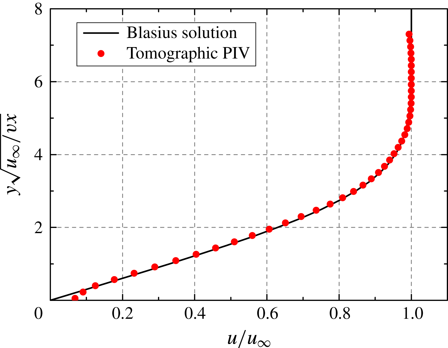
, 430 mm from the leading edge) in order to verify that the boundary layer develops in the laminar regime along the entire domain of interest. The velocity profile is compared with the theoretical solution based on Blasius self-similarity (White Reference White1991) yielding a good agreement, which confirms the laminar regime of the undisturbed boundary layer (see figure 3). Near the wall (
 ${\it\eta}<0.1$
) the measured velocity profile deviates from the theoretical result due to the limited spatial resolution (Kaehler, Scharnowski & Cierpka Reference Kaehler, Scharnowski and Cierpka2012). The r.m.s. fluctuations of the streamwise velocity component do not exceed
 $2\,\%$
of the free-stream velocity, which also gives an indication of the current measurement noise level.
Undisturbed boundary layer profile measured at
 $x/h=70$
and comparison with Blasius solution.

4 Transitional flow past the micro-ramp
4.1 Mean flow organization
The topology of the time-averaged flow is obtained by analysing the mean velocity and vorticity fields, which in turn provide a baseline for interpreting the instantaneous flow pattern. The mean velocity and vorticity fields are obtained by averaging 200 instantaneous uncorrelated snapshots. The cross-flow velocity is inspected at three
 $y$
–
 $z$
planes positioned downstream of the micro-ramp at
 $x/h=5$
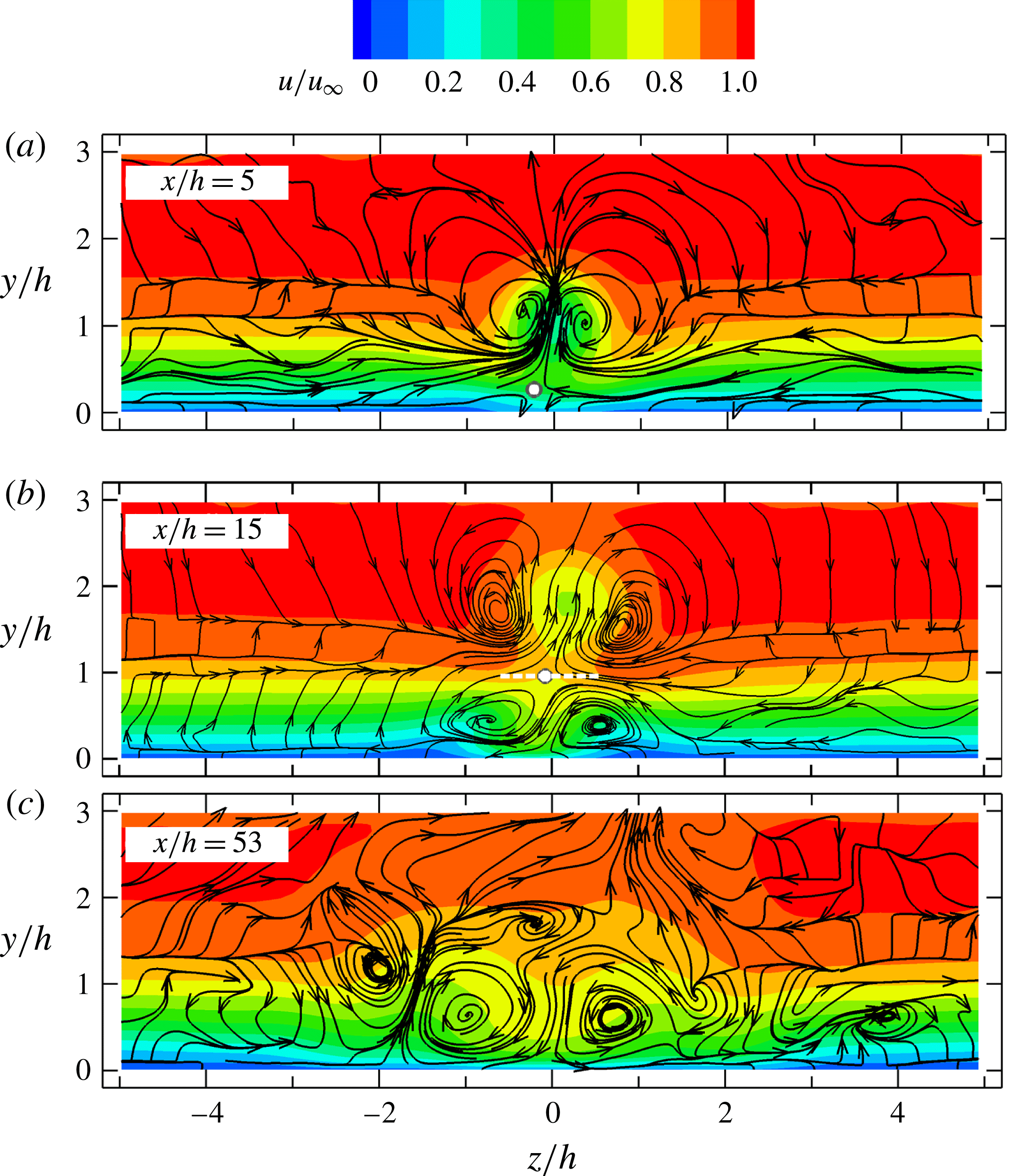
, 15 and 53. The result is illustrated in figure 4, where the projection of the streamlines on the
 $y$
–
 $z$
plane is visualized along with the colour contours of the non-dimensional streamwise velocity (
 $u/u_{\infty }$
).
Time-averaged streamwise velocity (colour contours) and flow topology (streamtraces) in the
 $y$
–
 $z$
plane at three streamwise locations. The stagnation point in (a,b) highlighted with white dot, the ‘neck’ region in (b) shown with white-dash line.

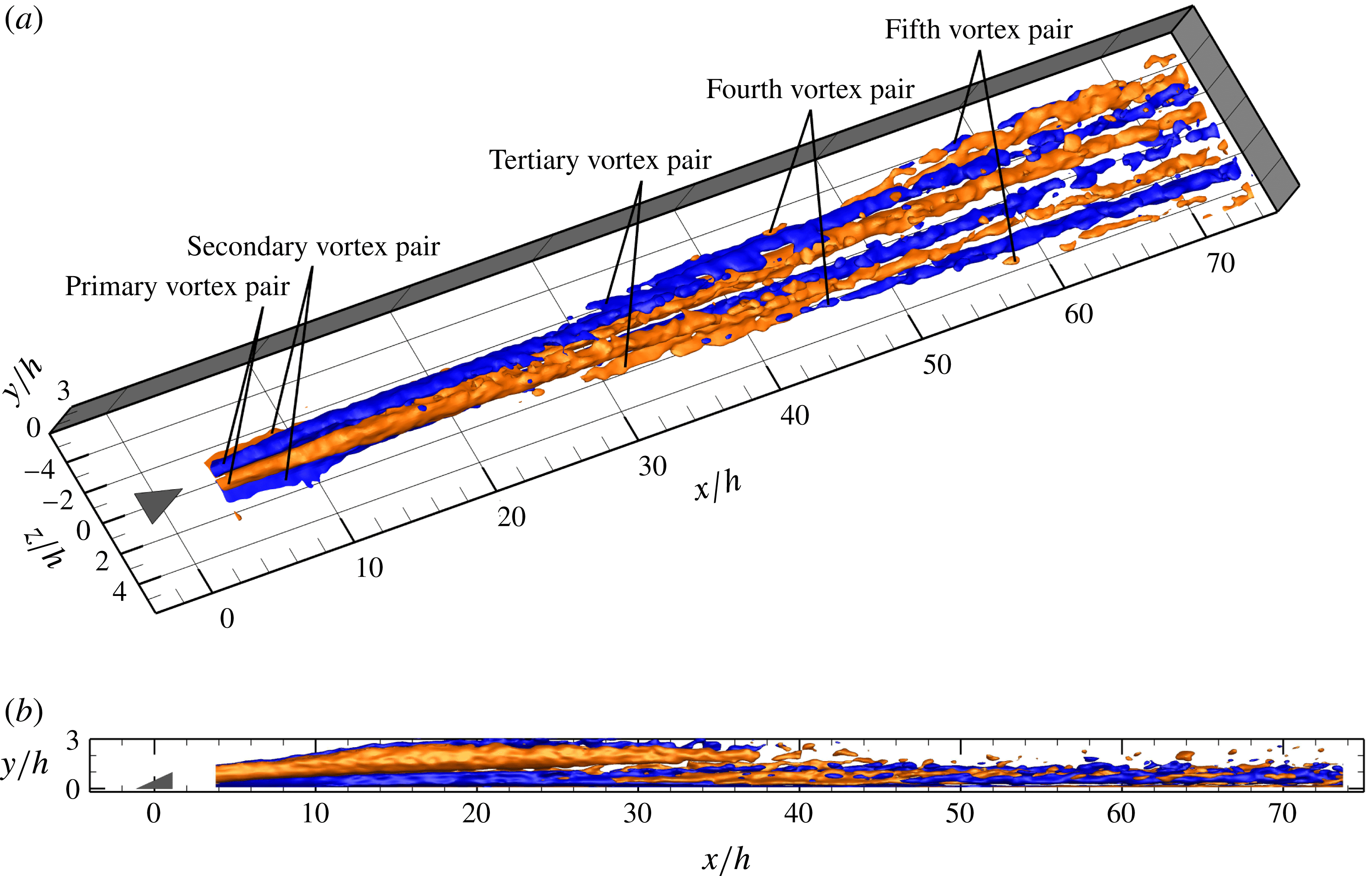
Three-dimensional rendering of time-averaged streamwise vorticity (blue for anticlockwise rotation vortices,
 ${\it\omega}_{x}^{\ast }=-0.04$
; red for clockwise rotation vortices,
 ${\it\omega}_{x}^{\ast }=0.04$
). Perspective (a) and side (b) view.

In the near-wake region (
 $x/h=5$
), the micro-ramp induces a pair of counter-rotating vortices (primary streamwise vortex pair), which produce a central upwash motion and a lateral downwash at
 $z/h=\pm 0.6$
(shown with the projected streamlines in figure 4
a). This pattern has been reported in numerous studies conducted in supersonic turbulent boundary layers (Babinsky et al.
Reference Babinsky, Li and PittFord2009; Sun et al.
Reference Sun, Schrijer, Scarano and van Oudheusden2012). The pronounced upwash motion induced by this primary vortex pair causes a mushroom-shaped velocity deficit region around the symmetry plane (
 $z/h=0$
) and the formation of a saddle point at approximately
 $y/h=0.2$
(shown as the white dot). The flow in the region below the saddle point is directed towards the wall where it stagnates. The wall-normal position of the vortex core appears at
 $y/h=1.2$
for
 $x/h=5$
(figure 4
a) and is lifted up to
 $y/h=1.8$
downstream at
 $x/h=15$
(figure 4
b) as a result of the self-induced velocity (Crow Reference Crow1970). With the primary vortex pair being lifted up (
 $x/h=15$
), the stagnation point emerges away from the wall to approximately one micro-ramp height. A second pair of counter-rotating vortices is formed (approximately at
 $z/h=\pm 0.7$
), with opposite rotation direction with respect to the primary pair. Secondary vortices were also observed by Tirtey et al. (Reference Tirtey, Chazot and Walpot2011) in the hypersonic laminar micro-ramp wake. The presence of this vortex pair induces a downwash motion at the symmetry plane close to the wall, which tends to flatten the velocity profile (see figure 6
b). As a result, high momentum fluid is directed downwards below the stagnation point with a twofold increase of the velocity close to the wall (figure 6
b,
 $y/h=[0.1,0.2]$
,
 $x/h=15$
). The high-speed region between the secondary vortices also emphasizes the formation of a neck region (indicated by a white dashed line) at approximately
 $y/h=1.0$
(
 $x/h=15$
, figure 4
b). Lateral upwash produced by the secondary vortex pair generates low-speed regions and associated velocity deficit at the side. The large increase in wall shear, in combination with the inflectional velocity profile (
 $y/h=0.5$
,
 $z/h=\pm 1$
), is associated to determining triggering conditions for the instability mechanism leading to flow transition, which is further circumstantiated in § 4.3. At
 $x/h=53$
(figure 4
c), the strength of the primary vortex can no longer be detected by the streamlines as they appear to have risen beyond the upper boundary of the measurement domain. From figure 5, it appears that the primary vortices do remain at a constant height close to the measurement boundary, but with a significant decay of the peak vorticity. The foci of the secondary vortex pair have moved outwards in spanwise direction widening the high-speed region close to the wall. Two low-speed regions are formed at the spanwise location of the latter vortex pair. A weaker tertiary vortex pair is induced aside the secondary pair with the same sense of rotation as the primary one (see figure 5). The combined effect of secondary and tertiary vortices causes focused ejections of low-speed fluid above the wall, which is associated to the formation of unstable hairpin structures as will be discussed in the remainder of the study.
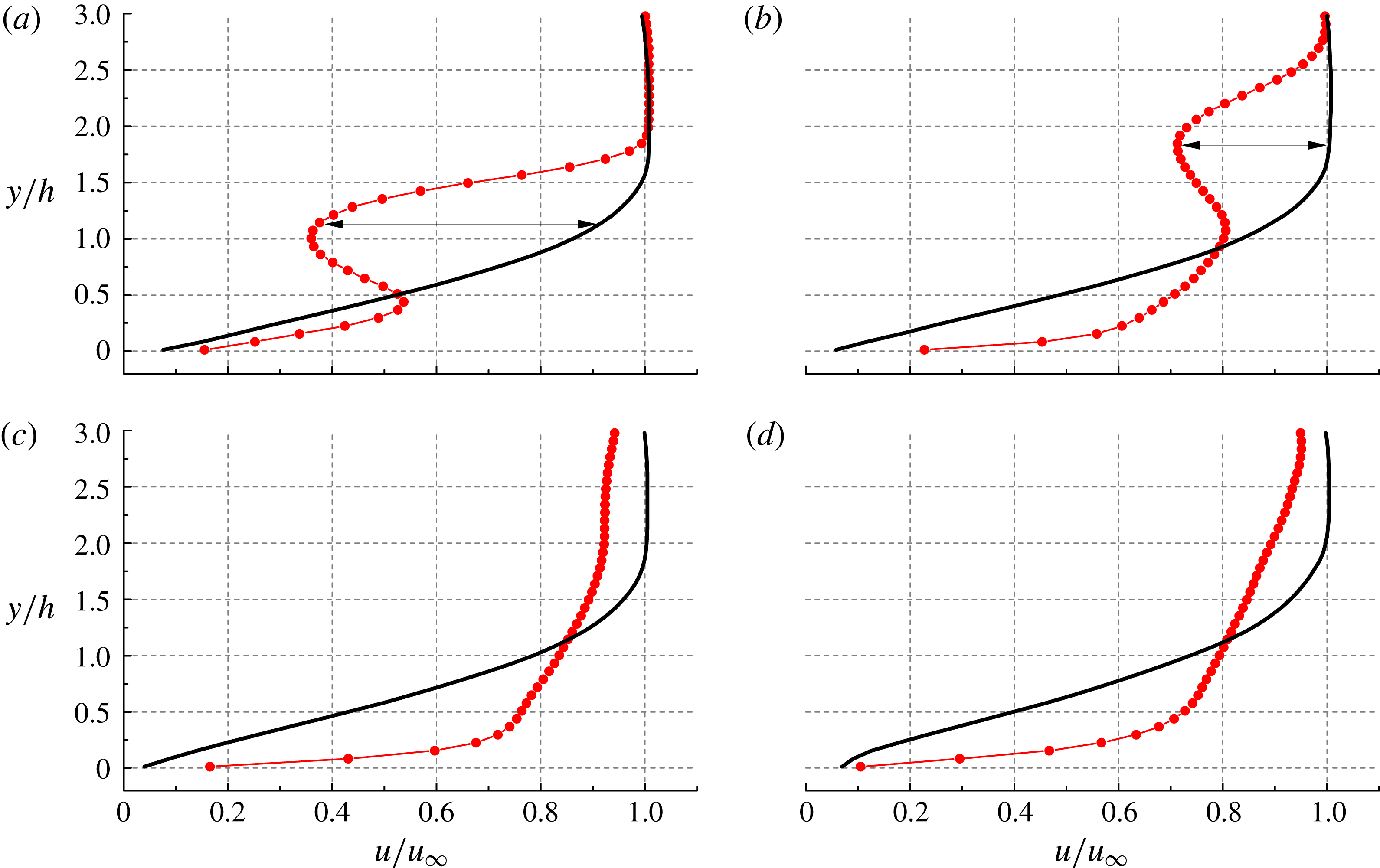
Streamwise evolution of time-averaged velocity profile in the symmetry plane (red line-circle) and comparison with undisturbed boundary layer profile (black line). (a)
 $x/h=5$
, (b)
 $x/h=15$
, (c)
 $x/h=40$
, (d)
 $x/h=70$
.

The time-averaged vortex topology is rendered in figure 5 through the spatial distribution of non-dimensional streamwise vorticity (
 ${\it\omega}_{x}^{\ast }={\it\omega}_{x}h/u_{\infty }$
). Close to the micro-ramp, two pairs of counter-rotating structures corresponding to the primary and secondary vortex pair are clearly identified. The vortex system persists downstream with decreasing strength. The lift-up and diffusion process of the primary vortices is evident from the side view (figure 5
b). The secondary vortex pair appears to be active from the most upstream measurement location. The tertiary system of vortices makes its first appearance outwards at approximately
 $x/h=25$
. It is hypothesized here that the tertiary vortex structure might be the precursor to the laminar-to-turbulent transition as it produces together with the secondary vortex pair the two saddle points close to the wall with upwash regions potentially generating unsteady ejection events. This hypothesis is further elaborated in the discussion of the statistical flow properties (§ 5). Further downstream, even a fourth (
 $x/h=40$
) and a fifth (
 $x/h=54$
) vortex pair are observed outwards of the tertiary vortex pair. These vortices are ascribed to the mutual induction effect of the neighbouring vortices. The whole vortical pattern follows the shape of a wedge, in analogy to that shown in turbulent wedge.
4.2 Momentum deficit and log-layer
Previous studies of the micro-ramp wake have dealt with the streamwise evolution of the momentum deficit and characterized its turbulent recovery (Ghosh, Choi & Edwards Reference Ghosh, Choi and Edwards2010; Sun et al.
Reference Sun, Schrijer, Scarano and van Oudheusden2014b
). In the present case, the momentum deficit and the properties of the shear layer induced by the micro-ramp pertain to the laminar regime and the velocity profile in the symmetry plane (
 $z/h=0$
) is compared with that of the undisturbed boundary layer.
The situation is illustrated at four streamwise positions (
 $x/h=5$
, 15, 40 and 70) in figure 6. The micro-ramp wake exhibits an overall deficit with respect to the laminar reference of approximately
 $0.6u_{\infty }$
at
 $x/h=5$
with a minimum velocity located at
 $y/h=1.2$
. Two shear layers bound the region of reduced momentum. The upper shear layer emanates from the trailing edge of the micro-ramp, which eventually becomes unstable with the formation of K–H vortices (Acarlar & Smith Reference Acarlar and Smith1987). The bottom shear layer is produced by the combined action of the primary and secondary vortex pair transporting high momentum fluid towards the symmetry plane. As the streamwise velocity locally exceeds that of the undisturbed boundary layer, a higher near-wall shear is produced. The rapid decrease of the velocity deficit (
 $0.3u_{\infty }$
at
 $x/h=15$
,
 $y/h=1.8$
) indicates a recovery process dominated by the large-scale mixing across the shear layer. At
 $x/h=40$
and 70 (figure 6
c,d), no velocity minimum can be observed in the profile, which is ascribed to the combined effect of the diffusion of the wake induced by shear layer mixing and the upward motion of the primary vortex pair approaching the upper boundary of the measurement domain. However, the local velocity deficit observed at the edge of the undisturbed boundary layer is considered to be caused by the strong upward motion of the secondary and tertiary vortices. This effect is confined in a limited spanwise range (
 $z/h=[-5,5]$
) and outside of it, the full free-stream velocity is observed (see figure 4).
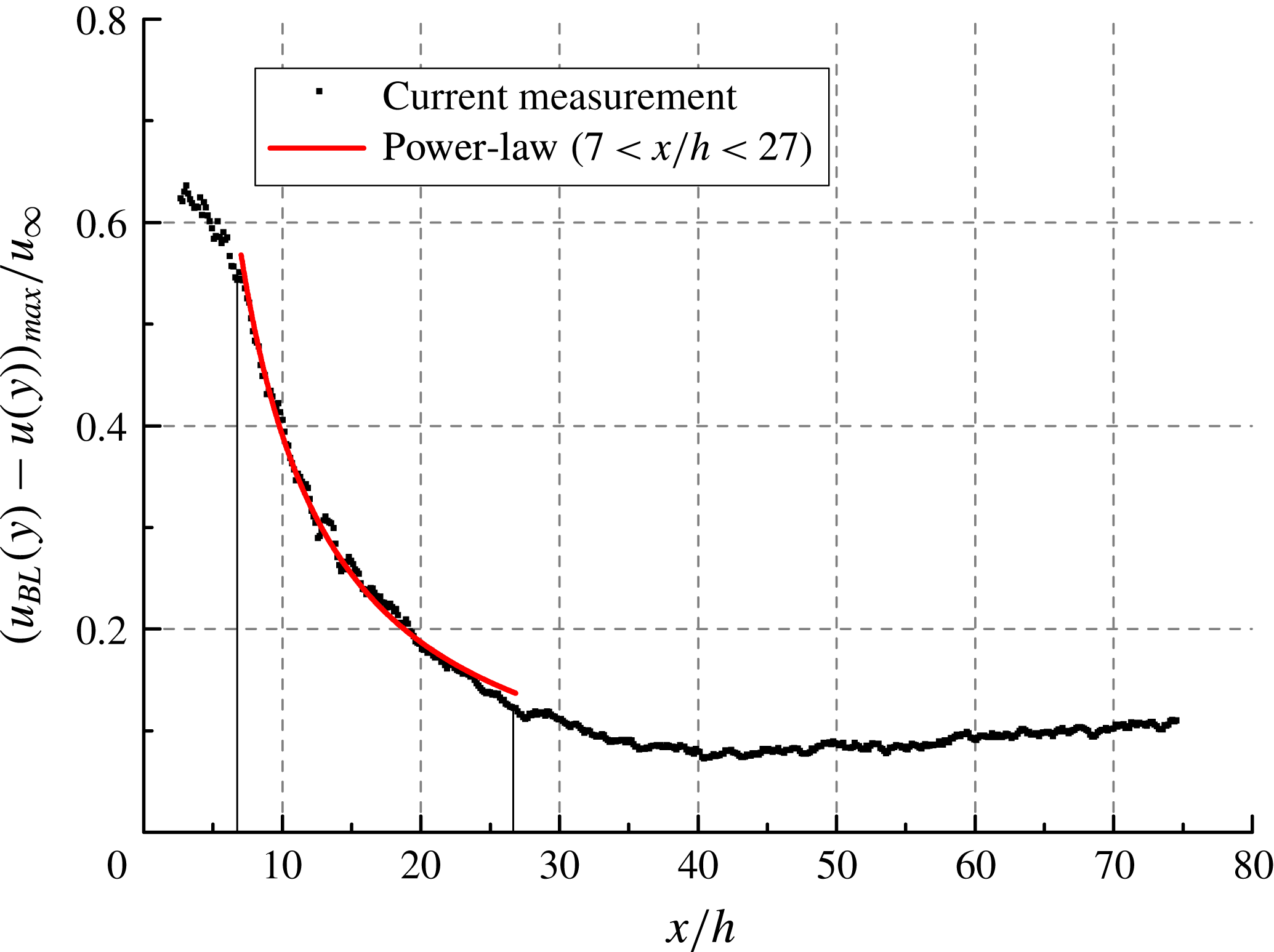
The wake recovery is quantified by following the streamwise evolution of the maximum momentum deficit. A rapid decreasing rate of maximum velocity deficit
 $(u_{BL}(y)-u(y))_{max}/u_{\infty }$
(where
 $u_{BL}$
is the velocity of undisturbed boundary layer) from
 $0.6u_{\infty }$
to
 $0.1u_{\infty }$
occurs within the range of
 $x/h<35$
. Past this range, the velocity deficit is confined to the upper region of the boundary layer and stays constant at approximately
 $0.1u_{\infty }$
. Sun et al. (Reference Sun, Schrijer, Scarano and van Oudheusden2014b
) observed that the streamwise evolution of the maximum velocity deficit follows a power-law type decay in a supersonic turbulent boundary layer. In the present case the validity of the power-law decay is confirmed by the acceptable fit to velocity deficit profile (figure 7) in the range
 $x/h=[7,27]$
, where the wake recovery is dominated by the K–H vortex structures. A detailed analysis of the latter is given in the next section. The power-law relation reads as:
 $$\begin{eqnarray}\frac{(u_{BL}(y)-u(y))_{max}}{u_{\infty }}=4.5\left(\frac{x}{h}\right)^{-1.06}.\end{eqnarray}$$
Streamwise evolution of maximum velocity deficit
 $(u_{BL}(y)-u(y))_{max}/u_{\infty }$
.

The recovery rate of 1.06 is considerably larger than the values of 0.73–0.78 reported by Sun et al. (Reference Sun, Schrijer, Scarano and van Oudheusden2014b ), indicating a more efficient momentum mixing. The latter is ascribed to the longer persistence of coherent large-scale flow structures occurring in the laminar regime, as opposed to the more rapid breakdown in the turbulent boundary layer.
Wall-normal semi-logarithmic profile of
 $u/u_{\infty }$
developing streamwise along the symmetry plane (black squares). Log-law region highlighted with dashed red line. (a)
 $x/h=5$
, (b)
 $x/h=15$
, (c)
 $x/h=25$
, (d)
 $x/h=40$
, (e)
 $x/h=53$
, (f)
 $x/h=70$
.

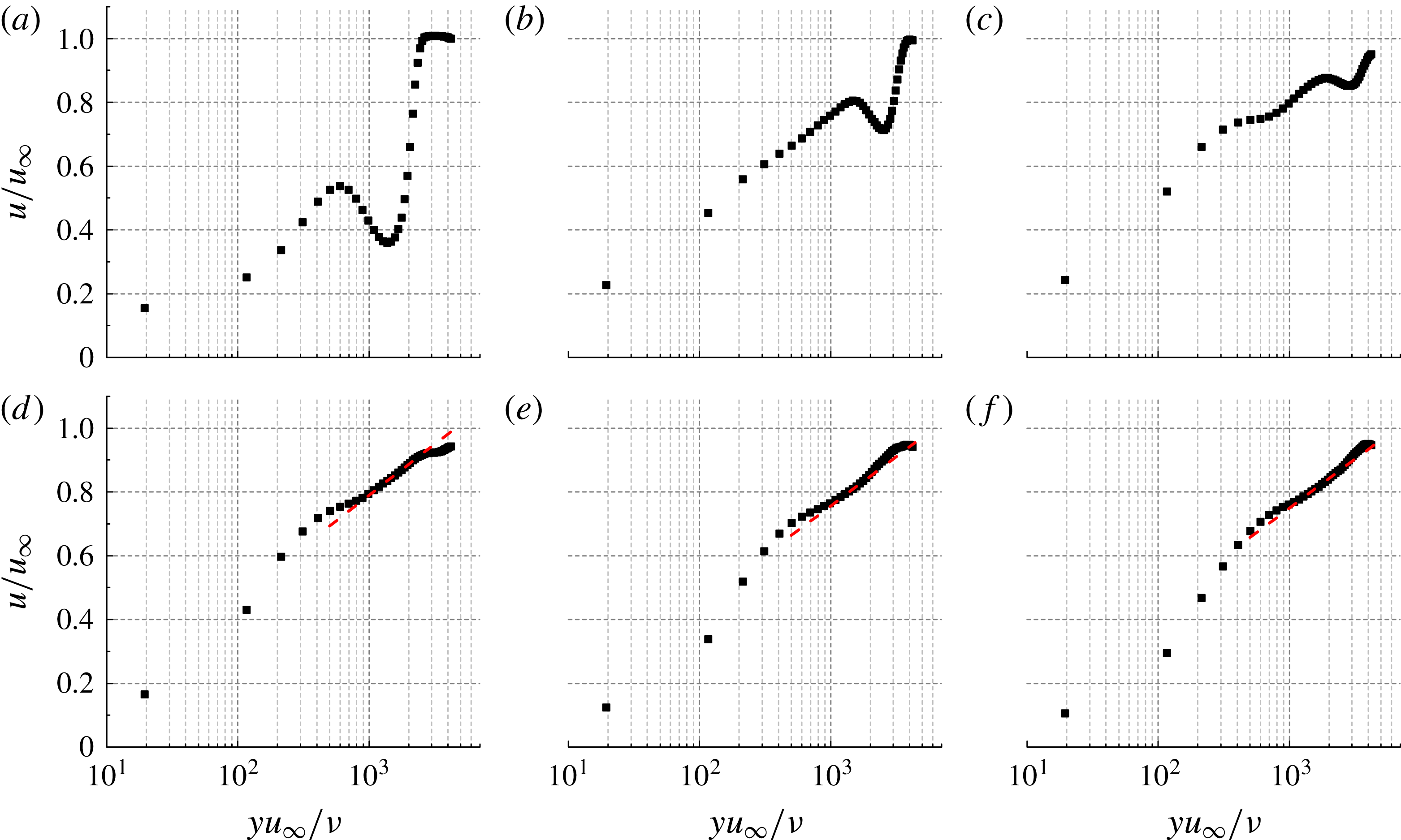
In order to establish the onset and development of the turbulent regime, the velocity profile is plotted in the semi-logarithmic scale enabling a direct comparison with the log-law fit. Figure 8 illustrates the streamwise development of non-dimensional velocity
 $u/u_{\infty }$
versus
 $u_{\infty }y/{\it\nu}$
along the symmetry plane. The logarithmic equation characterizing the overlap layer of turbulent boundary layer reads as (Kline, Coles & Hirst Reference Kline, Coles and Hirst1969):
 $$\begin{eqnarray}u^{+}=\frac{1}{{\it\kappa}}\ln y^{+}+B,\end{eqnarray}$$
where
 ${\it\kappa}=0.41$
,
 $B=4.0$
. Substituting
 $u_{{\it\tau}}/u_{\infty }=(1/2c_{f})^{1/2}$
into (4.2) yields
 $$\begin{eqnarray}\frac{u}{u_{\infty }}=A\ln \frac{u_{\infty }y}{{\it\nu}}+C,\end{eqnarray}$$
where
 $$\begin{eqnarray}A=\frac{1}{{\it\kappa}}\left(\frac{1}{2}c_{f}\right)^{1/2}\end{eqnarray}$$
and
 $$\begin{eqnarray}C=\left(\frac{1}{2}c_{f}\right)^{1/2}\left[\frac{1}{2{\it\kappa}}\ln \left(\frac{1}{2}c_{f}\right)+B\right].\end{eqnarray}$$
At
 $x/h=5$
, 15 and 25, the lower part of the profile features the large momentum defect region due to the wake. At
 $x/h=40$
, 53 and 70, a linear range of
 $u_{\infty }y/{\it\nu}=[1\times 10^{3},2\times 10^{3}]$
in the upper part of the profile indicates the presence of an overlap layer complying with the log law. By using (4.3), the skin friction
 $c_{f}$
is determined by a linear fit in the log region, shown by the red dashed line in figure 8. Consequently, the flow exhibits turbulent regime from
 $x/h=40$
.
4.3 Instantaneous flow organization
The formation and growth of unstable oscillations past the isolated roughness elements have been associated in the past to one of the driving mechanisms forcing boundary layer transition. Extensive discussion is found in the literature that focuses on shear layer instability past isolated roughness elements of various geometries, such as circular cylinders (Ergin & White Reference Ergin and White2006) and hemispherical cap (Acarlar & Smith Reference Acarlar and Smith1987; Citro et al.
Reference Citro, Giannetti, Luchini and Auteri2015). This instability is conjectured to act as precursor to the onset of transition. In the case of micro-ramps, the onset of shear layer instability was also observed in supersonic turbulent boundary layers (Li & Liu Reference Li and Liu2011; Sun et al.
Reference Sun, Schrijer, Scarano and van Oudheusden2012). On the other hand, different conclusions were drawn by Choudhari et al. (Reference Choudhari, Li and Edwards2009), who examined the role of both shear layer and streak instabilities in a supersonic boundary layer. The latter were associated to spanwise high shear layer of the flow, undergoing a more rapid growth compared to shear layer instability away from the roughness element and triggering final breakdown to turbulence. The current experiments visualize the instantaneous three-dimensional structure of velocity and vorticity fluctuations, from which the pattern of K–H vortices can be observed along with their evolution in the wake. The instantaneous vortex structure is highlighted from the three-dimensional isosurface of a vortex detection criterion by
 ${\it\lambda}_{2}$
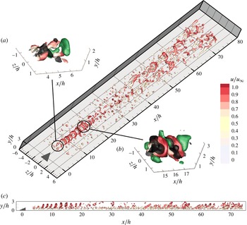
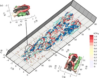
(Jeong & Hussain Reference Jeong and Hussain1995). The isosurface in figure 9 is colour coded by streamwise velocity to better distinguish between the portions of flow at high speed and at low speed. Two supplementary movies (Movies 1 and 2) of 20 uncorrelated snapshots are available at http://dx.doi.org/10.1017/jfm.2016.120 showing the perspective and side view of the flow pattern.
The instantaneous flow pattern detected by
 ${\it\lambda}_{2}$
criterion colour coded by
 $u/u_{\infty }$
: (a,b) perspective view, ejection (black) and sweep (green) events are shown by
 $u^{\prime }v^{\prime }/u_{\infty }^{2}=-0.002$
; (c) side view.

4.3.1 Evolution of K–H vortices
In the very near wake of the micro-ramp (
 $x/h<4$
), the shear layer on top of the wake exhibits a quasi-steady behaviour with no evidence of shear layer fluctuations. The baseline flow is dominated by the primary streamwise vortex pair (see figure 5). Downstream of the very near-wake region, unstable waves in the shear layer due to K–H instability are observed, leading to large-scale quasi-periodic fluctuations at the upper shear layer. A very similar wavy structure has been observed in numerous studies dealing with a turbulent boundary layer upstream of the micro-ramp (Li & Liu Reference Li and Liu2010; Sun et al.
Reference Sun, Schrijer, Scarano and van Oudheusden2012). Moreover, the presence of K–H vortices producing shear layer fluctuations is consistent with the inflection point in the mean velocity profile immediately downstream of the micro-ramp (see figure 6
a,
 $x/h=5$
).
The arc-shaped vortices within the shear layer emanating from the micro-ramp trailing edge can be clearly observed in figure 9(a) (Movie 1). The low momentum fluid ejection event (Q2,
 $u^{\prime }<0,v^{\prime }>0$
) associated with an arc vortex is visualized with isosurface of
 $u^{\prime }v^{\prime }/u_{\infty }^{2}=-0.002$
(coloured black). The sweep events (Q4,
 $u>0,v<0$
) are also identified as isosurface of
 $u^{\prime }v^{\prime }/u_{\infty }^{2}=-0.002$
(coloured green). Q2 events focus within the leg portion and upstream region of the arc-vortex head (Zhou et al.
Reference Zhou, Adrian, Balachandar and Kendall1999), whereas the sweeping motions (Q4) are more broadly distributed in the region downstream of the vortex head and mildly shown along the sides of legs (Adrian & Liu Reference Adrian and Liu2002). Further downstream, the vortices develop a quasi-streamwise leg-like portion (Robinson Reference Robinson1991), which elongate under the shearing motion between the head and the near-wall region. The overall pattern features a train of hairpin-like vortices. The spanwise rotation of the head portion induces an inclination angle of approximately
 $35^{\circ }{-}60^{\circ }$
of the leg portion to the
 $x$
axis, which agrees fairly well with the hairpin vortex organization investigated by Adrian, Meinhart & Tomkins (Reference Adrian, Meinhart and Tomkins2000). Moving downstream, the K–H vortices lift up, due to the upwash motion induced by the leg portion, and form an inclined shear layer. At
 $x/h=15$
, the K–H vortices appear to grow in size and to increase their azimuthal range due to self-induction of the legs. Eventually, the leg pairs connect at the bottom to produce full ring vortices, as shown in figure 9(b) (Movie 1) and observed in previous studies (Sun et al.
Reference Sun, Scarano, van Oudheusden, Schrijer, Yan and Liu2014a
; Yan et al.
Reference Yan, Chen, Wang and Liu2014). The random traces of small-scale vortices near the wall (
 $y/h<0.5$
), are solely ascribed to the effect of measurement noise.
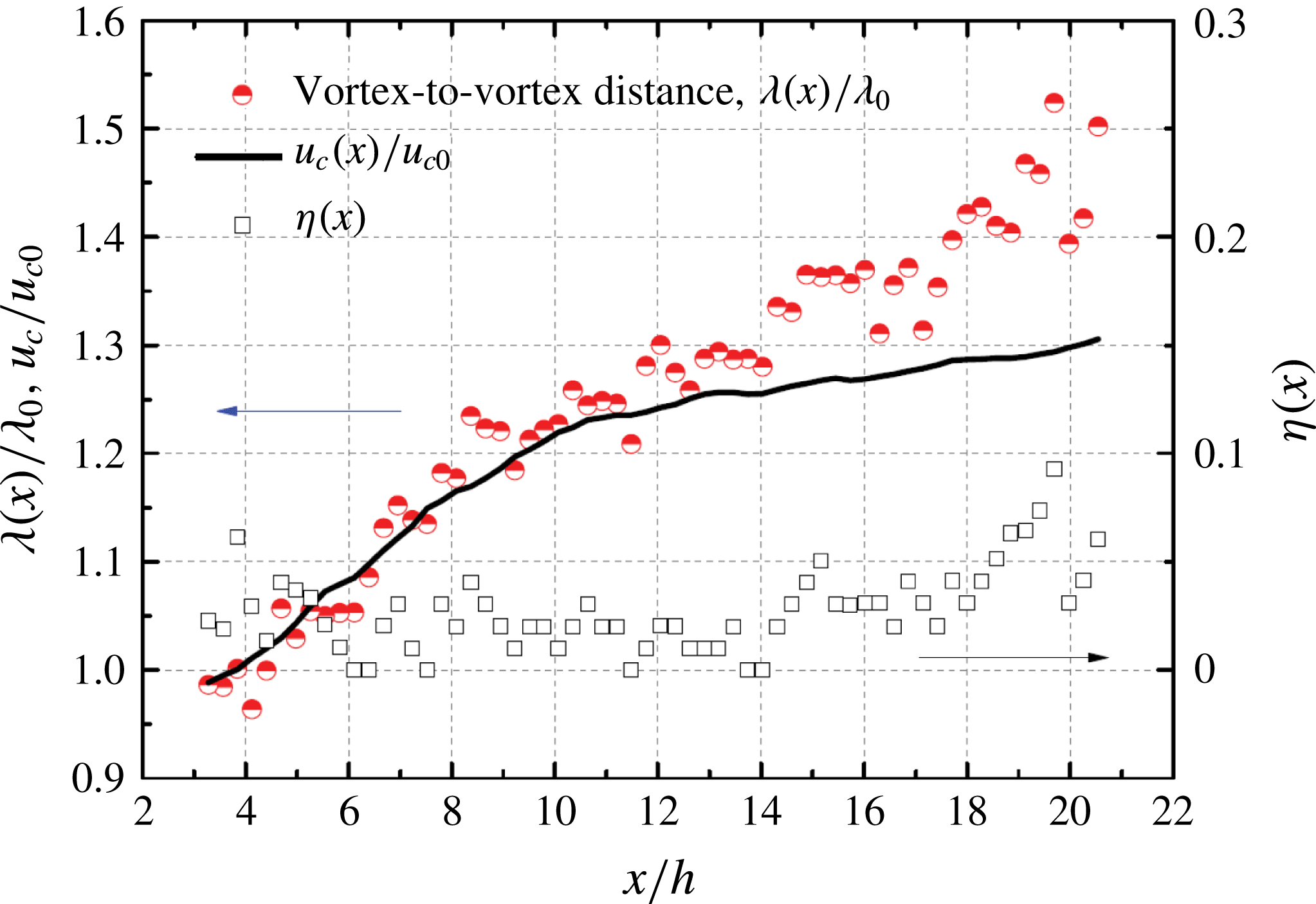
The wavelength of the shear layer fluctuations induced by the K–H vortices is defined as the interval between adjacent vortices. A statistical analysis by means of the spatial autocorrelation function is applied to the instantaneous spanwise vorticity field (
 ${\it\omega}_{z}$
). The region over which the spatial autocorrelation is evaluated is
 $6.4h$
in the streamwise direction. The ensemble-averaged wavelength is evaluated over a set of 100 instantaneous snapshots in the range of
 $x/h=[4,20]$
, as shown in figure 10. The vortices are spaced at regular intervals of approximately
 ${\it\lambda}_{0}/h=1.45$
in the range of
 $x/h=[4,6]$
, which is the initial wavelength (see figure 9
c, side view). The convection velocity of the vortices can be inferred by invoking Galilean decomposition with respect to the local streamwise velocity (Adrian et al.
Reference Adrian, Meinhart and Tomkins2000). The initial convection velocity estimated from the vortex centre is
 $u_{c0}=0.69u_{\infty }$
. The resulting frequency of vortex shedding is then estimated to be
 $f_{s0}=u_{c0}/{\it\lambda}_{0}=2430~\text{Hz}$
corresponding to a Strouhal number of
 $St_{0}=f_{s0}h/u_{\infty }=0.48$
. Klebanoff et al. (Reference Klebanoff, Cleveland and Tidstrom1992) reported that the Strouhal number in the wake of roughness elements strongly depends on their size, shape and Reynolds number. Several studies (Acarlar & Smith Reference Acarlar and Smith1987; Klebanoff et al.
Reference Klebanoff, Cleveland and Tidstrom1992) investigating the shedding phenomenon from roughness elements report Strouhal numbers varying from 0.2 to 0.5. The current experiment falls near the upper end of the range.
Streamwise evolution of vortex-to-vortex distance. Non-dimensional convective velocity
 $u_{c}/u_{c0}$
(black solid line), non-dimensional wavelength
 ${\it\lambda}/{\it\lambda}_{0}$
(red circles) and the vortex pairing probability
 ${\it\eta}(x)$
(square).

The streamwise evolution of the wavelength is compared with the increase of the convective velocity
 $u_{c}$
of the K–H vortices, in order to determine the occurrence of vortex paring. In the range of
 $x/h=[4,14]$
, the convective velocity increases from
 $u_{c0}=0.69u_{\infty }$
to
 $u_{c}=0.85u_{\infty }$
(
 $1.26u_{c0}$
). The wavelength has the same growth rate as the convective velocity, indicating that no vortex pairing takes place. However, in the later stage (
 $x/h=[14,18]$
), the growth of the wavelength departs from the convective velocity and exhibits a steeper increase than the convective velocity, leading to
 ${\it\lambda}/{\it\lambda}_{0}=1.4$
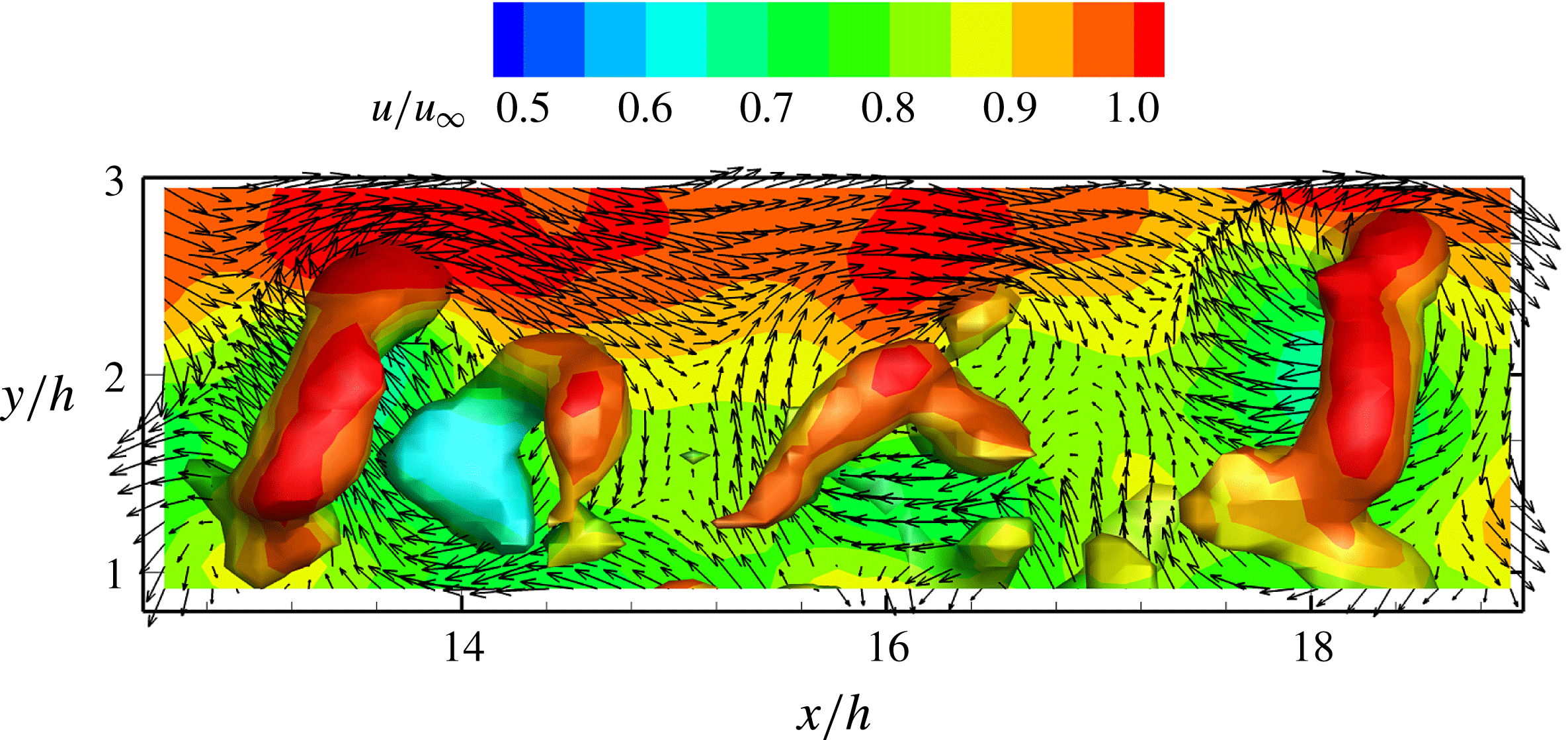
. In this stage, neighbouring ring vortices are observed to occasionally approach each other and undergo a rapid pairing, which can be observed in the zoomed view of instantaneous vortex structure in figure 11. The swirling pattern of velocity vectors becomes evident when displaying it after subtracting a convective velocity of
 $0.85u_{\infty }$
. The pairing process is observed to occur intermittently, therefore it does not lead, on average, to a doubling of the wavelength as evaluated from statistical cross-correlation analysis. In the range of
 $x/h=[18,20]$
, the interval of the vortices further increases to approximately
 ${\it\lambda}/{\it\lambda}_{0}=1.5$
. As the convective velocity has remained relatively unaltered, the increased spatial separation signifies an increased occurrence of pairing in the downstream region. A simplified model is given here which describes the streamwise evolution of vortex-to-vortex distance, where the convective velocity
 $u_{c}$
and the probability of vortex pairing are considered:
 $$\begin{eqnarray}{\it\lambda}(x)={\it\lambda}_{0}(1+{\it\eta}(x))\frac{u_{c}(x)}{u_{c0}}.\end{eqnarray}$$
In the above equation
 ${\it\eta}(x)$
is the pairing probability. The equation does not account for multiple pairing. As shown in figure 10, the evolution of the vortex pairing probability
 ${\it\eta}(x)$
starts to increases from
 $x/h=14$
, leading to the deviation of wavelength evolution from that of the convective velocity.
After the pairing region, which extends up to approximately
 $x/h=24$
, the vortices rapidly break down under the effect of azimuthal instabilities accelerated by the strain rate of the boundary layer (see figure 9). As a result, the ring-shaped vortices are distorted and split into fragments. No apparent periodicity is observed downstream of
 $x/h=25$
and the associated vortex activity in the upper portion of the measurement domain has no clear pattern with decaying incoherent vortex fragments.
Occurrence of vortex pairing detected by
 ${\it\lambda}_{2}$
criterion colour coded by
 $u/u_{\infty }$
. The streamwise velocity contour in the symmetry plane shown with swirling vector field after subtracting a convective velocity of
 $0.85u_{\infty }$
.

4.3.2 Formation of turbulent wedge
In the near-wall region, newly formed vortex structures are observed starting from
 $x/h=35$
. These structures have a hairpin shape with head (spanwise rotation) and leg (quasi-streamwise rotation) portions. Instead of holding spanwise symmetry, the hairpins are more frequently observed in a ‘cane’ shape (Guezennec, Piomelli & Kim Reference Guezennec, Piomelli and Kim1989). Unlike the flow topology near the micro-ramp, the vortex structures do not develop following constant spanwise position (
 $z/h=0$
). Furthermore, the hairpin vortices appear more frequently shifted away from the symmetry plane and develop downstream with a spanwise spreading, as illustrated in figure 12. The position of first occurrence of these vortex structures coincides with the range where the tertiary vortex pair is detected in the system of time-averaged streamwise vortices (see figure 5). However, as also illustrated in the snapshots of Movies 1 and 2, the inception of such hairpin vortices varies significantly streamwise (
 $x/h=[30,50]$
), indicating an intermittent behaviour. The newly formed hairpins stay at a relatively constant wall-normal position, and no clear periodicity can be inferred from their pattern. Moreover, near the symmetry plane, lower to no activity of large-scale coherent vortex structures are observed, indicating a more isotropic regime of turbulent fluctuations. Movie 3 of 20 uncorrelated snapshots is available to show the zoomed-in flow pattern in the wedge region.
Instantaneous flow pattern at the wedge region. Vortices visualized by isosurfaces of
 ${\it\lambda}_{2}$
, colour coded by
 $u/u_{\infty }$
; low-speed regions (light blue
 $u^{\prime }=-0.13u_{\infty }$
) and high-speed regions (dark blue
 $u^{\prime }=0.1u_{\infty }$
); (a,b) details of ejection (black) and sweep (green) are shown by
 $u^{\prime }v^{\prime }/u_{\infty }^{2}=-0.005$
.

Singer (Reference Singer1996) discussed the conditions governing the formation of hairpin vortices in a zero pressure gradient vorticity field and found that it requires strong upward ejections. A study on the correlation between the newly formed hairpin vortices, low- and high-speed regions and ejection and sweep events are necessary to further understand the evolution of instantaneous vortex structure in the downstream region. The low-speed region is characterized by a negative component of the streamwise velocity fluctuation
 $u^{\prime }=-0.13u_{\infty }$
, shown as the light blue isosurface in figure 12 (Movie 3). The majority of the hairpin structures are observed enclosing the elongated low-speed regions. The upward motion induced in the middle of the legs transports low-speed fluid from the wall to the upper part of the boundary layer. Such ejection events (isosurface of
 $u^{\prime }v^{\prime }/u_{\infty }^{2}=-0.005$
,
 $u<0,v>0$
) take place at the low-speed region, as shown in figure 12(a,b). Comparably mild high-speed regions appear on the outside of the legs and upstream of the head region. These features are highlighted with (dark blue) isosurfaces of positive streamwise velocity fluctuations (
 $u^{\prime }=0.1u_{\infty }$
,). The sweep event (isosurface of
 $u^{\prime }v^{\prime }/u_{\infty }^{2}=-0.005$
,
 $u>0,v<0$
) in this region moves the high momentum flow from the upper boundary layer to the lower part. The global scenario of entangled hairpin vortices in range of
 $x/h=[35,75]$
resembles a wedge shape, indicating a spanwise development of the vortical structures moving downstream.
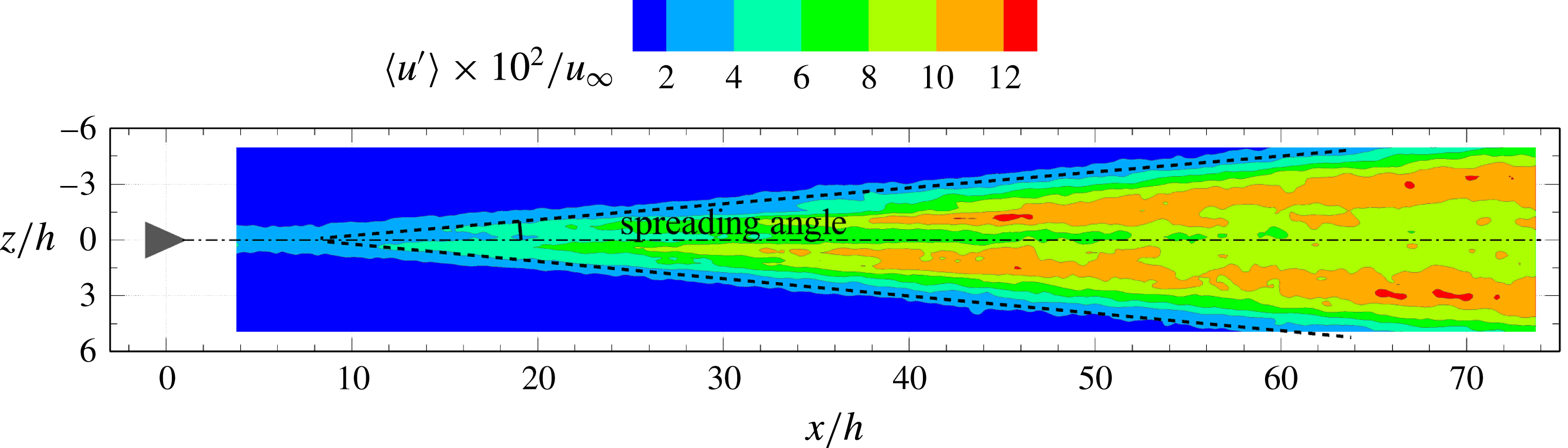
In fact, the process is very similar to that observed for the development of turbulent spots, where low-speed regions provide a favourable condition for perturbations to trigger flow instabilities, ultimately leading to transition (Singer Reference Singer1996; Durbin & Wu Reference Durbin and Wu2007). Furthermore, hairpin vortices have been reported as an ubiquitous phenomenon in turbulent spots (Ovchinnikov, Choudhari & Piomelli Reference Ovchinnikov, Choudhari and Piomelli2008; Wu & Moin Reference Wu and Moin2009). Consequently, the formation of a turbulent wedge can be confirmed in the current experiment, denoting the onset of boundary layer transition. By measuring the streamwise distance from the onset location of the newly formed hairpin vortices to the most downstream one in the measurement domain, the spreading angle is estimated to
 $4.5^{\circ }$
. A detailed analysis based on the statistical properties of the turbulent fluctuations is given in § 5.1.
4.3.3 Transition mechanisms
In summary, the evolutional flow pattern from the micro-ramp to boundary layer transition can be qualitatively divided into the following stages: (i) steady shear flow in the presence of streamwise vortices; (ii) formation and growth of K–H vortices; (iii) pairing and breakdown of hairpin or ring-shaped vortices; (iv) onset of new hairpin vortices close to the wall; (v) spanwise propagation of the turbulent interface bounding a wedge-like region.
The turbulent wedge appears downstream of the lift-up and breakdown process of K–H vortex structure. However, no evident relation is found between the arc-shaped vortices emanating from the micro-ramp trailing edge and the onset of these new hairpin vortices. Moreover, at the inception point of the latter structure, the fragmented K–H vortices have almost left the domain of interest and the distance between these two regions suggests no interaction taking place between them. The above discussion leads to the conclusion that the fluctuations occurring in the unstable shear layer past the micro-ramp trailing edge are not playing a role in the mechanism of transition.
It is instead conjectured, following the mean flow organization, that the inception of turbulent fluctuations is due to the near-wall secondary streamwise vortex pair, following the detachment of the primary pair. The boundary layer transition is associated to the excess wall shear induced by the secondary vortex pair, in combination with the inflectional velocity profile produced by the interaction with the tertiary vortex pair. The latter hypothesis is further discussed in the remainder of the study, and supported by the statistical analysis of the velocity field and its fluctuations.
5 Turbulent properties
The generation of turbulent fluctuations following a wedge-like pattern in the instantaneous results indicates that the onset of laminar-to-turbulent transition falls in the range of
 $x/h=[30,50]$
, which is captured within the current measurement domain. The evolution of the turbulence properties is investigated by analysing the r.m.s fluctuations of streamwise and wall-normal velocity (
 $u^{\prime },v^{\prime }$
) and turbulence production (
 $P$
).
5.1 Velocity fluctuations
The two reference states of the boundary layer are the fully laminar condition and the fully developed turbulent regime which can be characterized by a well-known distribution of streamwise velocity fluctuations. The analysis of the velocity fluctuations in the wake of micro-ramp focuses on its development starting from the conditions of the undisturbed boundary layer.
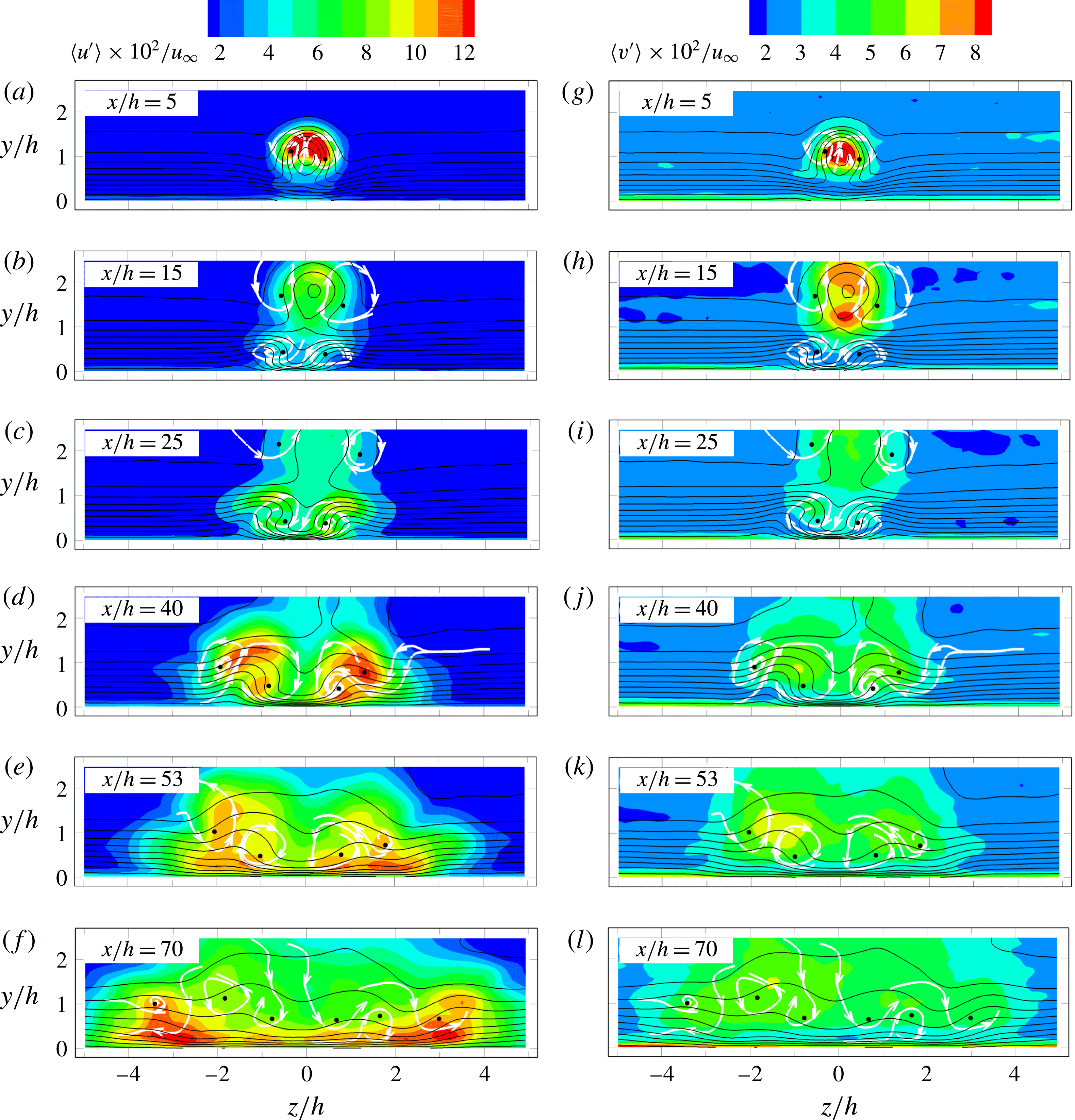
 $y$
–
 $z$
cross-sectional contour of velocity fluctuations ((a–f)
 $\langle u^{\prime }\rangle /u_{\infty }$
; (h–l)
 $\langle v^{\prime }\rangle /u_{\infty }$
), with contour lines of
 $u/u_{\infty }$
; selected projected streamlines: approximate location of time-averaged streamwise vortices, black dots: the vortex core.

The streamwise and wall-normal velocity fluctuations (
 $\langle u^{\prime }\rangle /u_{\infty },\langle v^{\prime }\rangle /u_{\infty }$
) are illustrated in figures 13 and 14. Colour contours of
 $y$
–
 $z$
cross-sections are selected at six streamwise locations
 $x/h=5,15,25,40,53,70$
and one
 $x$
–
 $y$
cross-section at the symmetry plane (
 $z/h=0$
). The
 $y$
–
 $z$
cross-sectional contours are superimposed with contour lines of time-averaged streamwise velocity. The location of the streamwise vortices is depicted by the selected projected streamlines. The upper and bottom inflection points of the streamwise velocity profile in the
 $y$
direction are plotted in the
 $x$
–
 $y$
cross-plane (see figure 14) to signify the edge of the near wake (
 $x/h<27$
), where the upwash induced by the primary vortex pair contributes to strong streamwise and wall-normal velocity fluctuations at the wake centre and interface of the wake and the free stream (also see figure 13
a,b,
 $x/h=5$
and 15). The maximum of the streamwise velocity fluctuations progressively lifts up and decreases in magnitude when travelling downstream, with a significant decay in the vortex breakdown region (
 $x/h>20$
) and a rapid wake recovery. From
 $x/h=30$
onwards, the velocity fluctuations in this region of the flow are considered to be negligible, or at least, they merge within the noise level of the measurement.
 $x$
–
 $y$
cross-sectional contour (
 $z/h=0$
) of streamwise velocity fluctuation,
 $\langle u^{\prime }\rangle /u_{\infty }$
;
 $y$
axis scaled by a factor of 1.2 for clarity.

Beneath the wake region, the downwash motion produced by the secondary vortex pair transports high momentum fluid towards the wall. This effect is already visible at
 $x/h=15$
(figure 13
b), where the contour lines near the wall in the symmetry plane are significantly bent downwards, resulting in a higher wall shear at that location. As a result, an increased level of streamwise velocity fluctuations is produced. Away from the symmetry plane, the secondary vortex pair induces ejection events, which produce low-speed regions, where an upward bent of the contour lines can be observed (also see figure 4
b,
 $x/h=15$
). A tertiary vortex pair is formed that produces jointly with the secondary pair a streamwise velocity profile exhibiting an inflection point. Unlike the decaying process of the inflectional profile (
 $u$
–
 $y$
profile) induced in the near wake past the micro-ramp, the latter persists until the most downstream measurement location and is considered to be the physical condition sustaining the cascade of fluctuations that lead to transition. As a result, the onset of a turbulent wedge is observed (corresponding with the formation of tertiary vortex pair) in this range (figure 13
b–f). In fact, in this case, the inflection point is significantly closer to the wall. The turbulent momentum mixing at the turbulent/non-turbulent interface results in a local maximum of streamwise velocity fluctuations (
 $\langle u^{\prime }\rangle /u_{\infty }$
) on top of the low-speed blob at
 $y/h=1,z/h=\pm 0.7,\pm 1.2$
and
 $\pm 1.7$
, corresponding to
 $x/h=25$
, 40 and 53 in figure 13(c–e). These local maxima are ascribed to the formation of large-scale hairpin-like coherent structures as also visualized in figures 9 and 12 (also see Movies 1 and 3). The wall-normal velocity fluctuations are less revealing. Their amplitude is approximately half that of the streamwise fluctuations (figure 13
g–l). However, the spatial distribution of
 $\langle v^{\prime }\rangle /u_{\infty }$
also returns a maximum in the near wake corresponding to the arc/ring vortices (figure 13
g,h,
 $x/h=5$
and 15) and two symmetrical peaks at the turbulent/non-turbulent interface tracing the boundaries of the turbulent wedge (figure 13
i–k,
 $x/h=25$
, 40 and 53). Also these statistical properties are in agreement with the hairpin vortex structures, especially the strong ejections at the hairpin head portion. In contrast, the flow region near the symmetry plane exhibits a comparatively lower level of fluctuations. The cross-sectional area occupied by turbulent fluctuations increases linearly in the spanwise direction due to the formation of the turbulent wedge. It is not yet understood whether the system of streamwise vortices emerging from the time-averaged analysis, which also features a wedge-like pattern, has an active role in this scenario, or is solely the statistical result of the staggered occurrence of hairpin vortices in the wedge.
Nearing the downstream edge of the investigated domain (figure 13
f,l,
 $x/h=70$
), the flow exhibits a more homogeneous distribution of the streamwise velocity fluctuations. However, the symmetrical peak of velocity fluctuations at the border of the turbulent wedge (
 $y/h=1,z/h=\pm 3.5$
) can still be distinguished, indicating the persistence of the hairpin vortices propagating towards the undisturbed boundary layer. Brinkerhoff & Yaras (Reference Brinkerhoff and Yaras2014) observed that the regeneration of wavepackets of hairpin vortices at the edge the turbulent spot dominates its lateral spreading. It is hypothesized here that the sidewise propagation of the turbulent/non-turbulent interface occurs by the formation of these large coherent hairpin structures rather than small-scale isotropic turbulent fluctuations. Further evidence is given in the following section by the analysis of turbulence production.
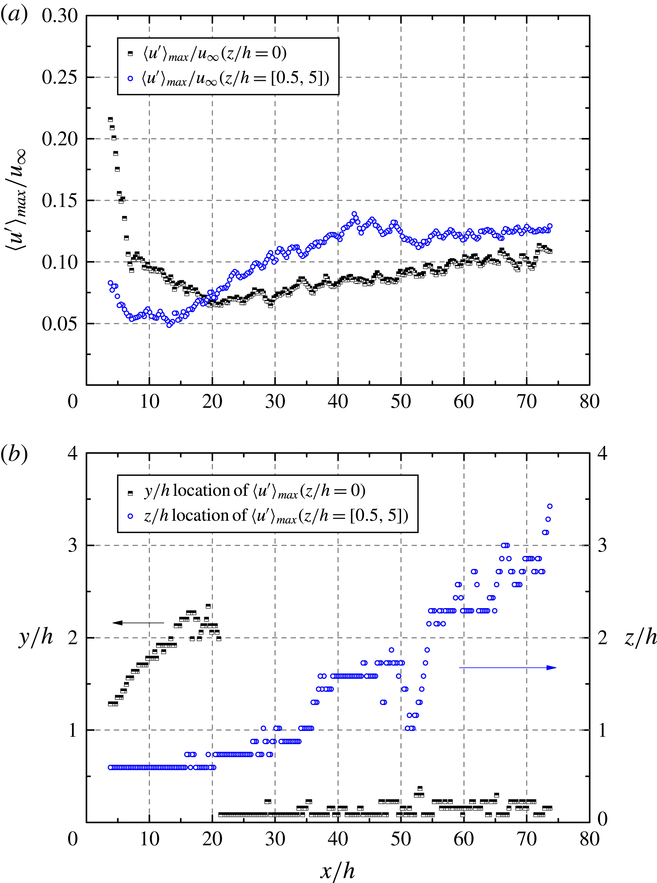
Maximum streamwise velocity fluctuation (
 $\langle u^{\prime }\rangle _{max}/u_{\infty }$
) evolution at
 $z/h=0$
(half solid black square) and
 $z/h=[0.5,5]$
(open blue circle). (a) Maximum velocity fluctuation magnitude at the symmetry plane and its sides (b) corresponding location of maxima along wall normal (
 $y/h$
) and spanwise (
 $z/h$
) direction.

The amplitude of the streamwise velocity fluctuations
 $\langle u^{\prime }\rangle$
is further evaluated by characterizing the evolution of its maximum both in the symmetry plane (
 $z/h=0$
) and away from it (
 $z/h=[0.5,5]$
). Figure 15 shows that in the upstream region
 $x/h=[3,20]$
, the streamwise velocity fluctuations are dominated at the symmetry plane by the shear layer instability, as confirmed by the location of the maximum (
 $y/h>1$
). The amplitude is rapidly decreasing in combination with the upward motion of the shear layer from upstream to downstream in this range. Beyond
 $x/h=20$
, the near-wall fluctuations intensify more rapidly along the wedge boundary rather than in the symmetry plane. This is followed by a spanwise dilation of the turbulent region indicating that hairpin vortices at the turbulent/non-turbulent interface dominate the velocity fluctuations. At the most downstream location, the distribution of streamwise velocity fluctuations tends to become more homogeneous and the maximum at the symmetry plane approaches the value at the wedge boundary around
 $0.12u_{\infty }$
. Although the values are distributed more homogeneously within the wedge in the spanwise direction, they are still in excess of values reported in turbulent boundary layers (Klebanoff Reference Klebanoff1955; Spalart Reference Spalart1988).
As the laminar-to-turbulent transition starts with the growth of a turbulent region, its spatial development is characterized by the spreading angle of the turbulent wedge (Schubauer & Klebanoff Reference Schubauer and Klebanoff1956), which is an important aspect to be further characterised. The r.m.s. of the streamwise velocity component (
 $\langle u^{\prime }\rangle /u_{\infty }$
) at a chosen
 $x$
–
 $z$
plane (
 $y/h=0.4$
) is shown in figure 16, where the turbulent wedge exhibits a marked increase of streamwise velocity fluctuations compared with the laminar region. Schubauer & Klebanoff (Reference Schubauer and Klebanoff1956) describe the turbulent wedge as consisting of a fully turbulent core bounded by an intermittent region. de Tullio (Reference de Tullio2013) studied the development of turbulent wedge using DNS and found that in the intermittent region, the turbulent kinetic energy (TKE) decreases sharply in comparison with the turbulent core. In the current study, a dramatic decrease of velocity fluctuation level can also be observed when moving from the turbulent core towards the boundary of turbulent wedge. The area of steep velocity fluctuation decrease is assumed to correspond to the intermittent region. A half spreading angle of approximately
 $4.6^{\circ }$
is found, which agrees fairly with
 $5.2^{\circ }$
reported in the numerical simulation of Brinkerhoff & Yaras (Reference Brinkerhoff and Yaras2014), where a micro-jet in cross-flow was used for triggering transition.
 $x$
–
 $z$
cross-sectional contour (
 $y/h=0.4$
) of streamwise velocity fluctuation,
 $\langle u^{\prime }\rangle /u_{\infty }$
.

5.2 Turbulence production
The source of velocity fluctuations is characterized here with the production of turbulent kinetic energy, which provides the energy extracted by the mean flow through the interaction of turbulent fluctuations and the shearing motion. Hereafter, the discussion focuses on the relation between coherent hairpin vortex structures and the production of turbulent kinetic energy. The production term follows the turbulent kinetic energy budget (Kundu & Cohen Reference Kundu and Cohen2002) as
 $$\begin{eqnarray}P=-\overline{u_{i}^{\prime }u_{j}^{\prime }}\,\frac{\text{d}\overline{u_{j}}}{\text{d}\overline{x_{i}}}.\end{eqnarray}$$
The turbulence production term is expressed in non-dimensional form
 $P^{\ast }$
by normalization with
 $u_{\infty }^{3}/h$
. The spatial distribution of
 $P^{\ast }$
is illustrated in figure 17 by colour contours in
 $y$
–
 $z$
cross-sections at six streamwise locations
 $x/h=5$
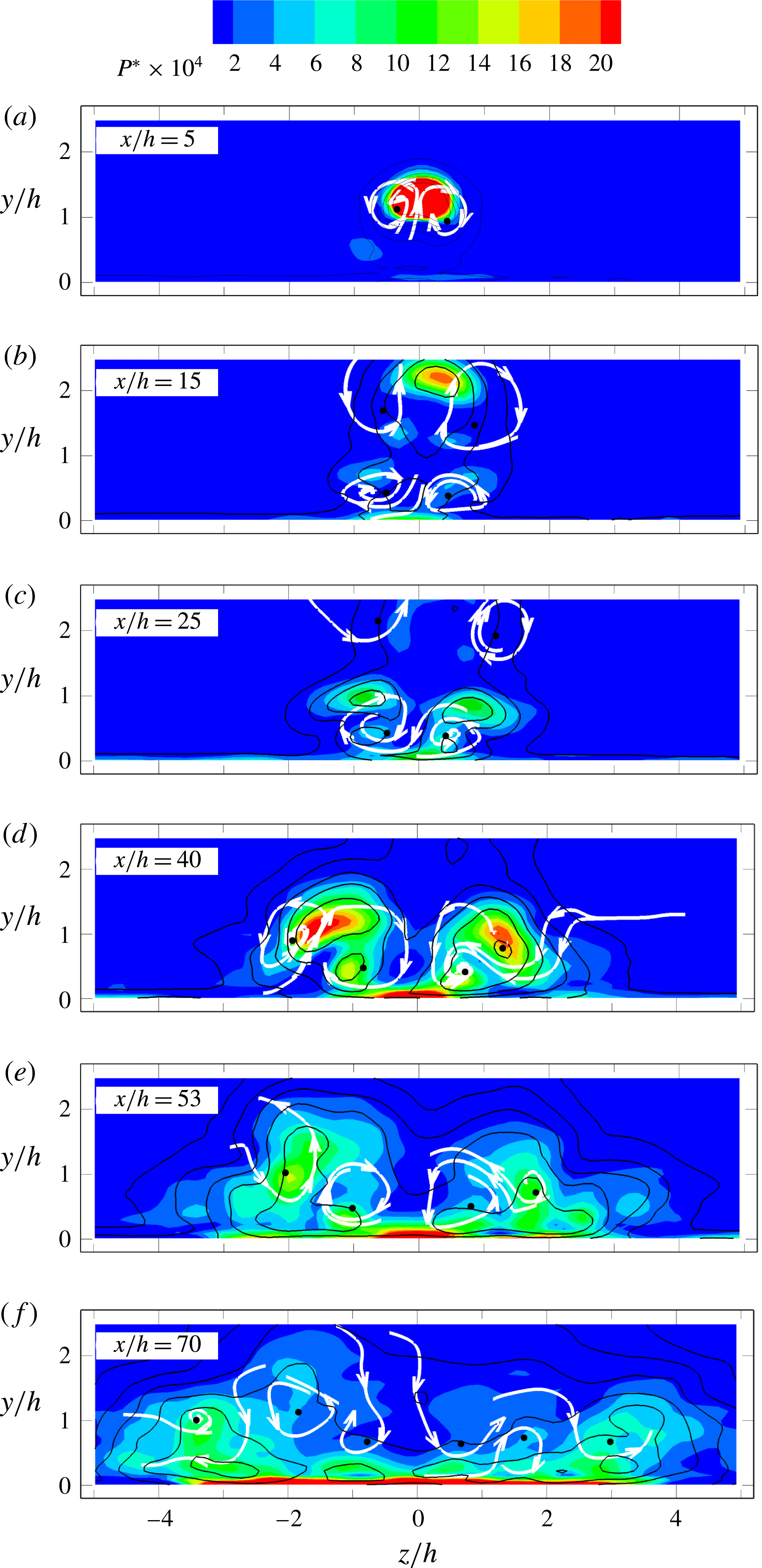
, 15, 25, 40, 53 and 70. Contour lines of the streamwise velocity fluctuation and the approximate location of the time-averaged streamwise vortices are added to ease the interpretation of results.
In the near wake (figure 17
a,b,
 $x/h=5{-}15$
), a maximum is attained within the upper shear layer dominated by the arc-shaped K–H vortices. At
 $x/h=15$
, a secondary peak of production is observed at the bottom shear layer in the region where K–H vortices form a ring shape. Following the wake recovery process, the production strength located both at the upper and bottom shear layer decreases rapidly and becomes negligible from
 $x/h=25$
(figure 17
c).
Close to the wall (figure 17
b,
 $x/h=15$
), a peak of production near the symmetry plane is identified initiated by the excess wall shear. At the same location two side peaks are observed slightly outwards and above the secondary vortices. The persistence of secondary vortices induces the tertiary vortex pair, contributing to sidewise ejections, which in turn sustain the sidewise shear layer. The latter is ascribed to be the feeding mechanism for the onset of velocity fluctuations, ultimately transferring mean flow energy into turbulent kinetic energy. The current experiment shows that the strength of turbulent production intensifies moving downstream and concentrates along the turbulent wedge boundary with a pattern becoming relatively complex as it features several maxima. The first peak value is associated to the region of flow ejection with maximum upwash motion (figure 17
b,
 $x/h=15,y/h=0.7,z/h=\pm 0.7$
). Another peak of turbulence production is observed close to the wall (more clearly resolved at
 $x/h=25$
and 40, figure 17
c,d), displaced towards the symmetry plane in comparison with the previous one. This maximum is ascribed to the increased wall shear induced by the secondary pair of streamwise vortices in the upstream region. At
 $x/h=40$
, the sideward movement of the turbulence production peaks is observed accompanying the spanwise propagation of the turbulent wedge. The location of turbulence production coincides with the boundary of the turbulent wedge, where a high occurrence of coherent hairpin vortex structures is found. This pattern is observed further downstream (figure 17
e,
 $x/h=70$
), indicating a self-similar behaviour for the turbulent wedge front. At
 $x/h=70$
also the turbulence production becomes relatively homogeneous with peak value close to the wall due to excess wall shear produced together by the secondary and tertiary vortices.
From the above scenario it can be concluded that the inception of turbulence production is given in the near-wake region by the secondary streamwise vortices with the combined effect of flow ejection and increased wall shear. Once established, the pattern is no longer dependent upon the secondary vortices as a cascade is produced along the edge of the turbulent wedge, where large-scale hairpin vortex structures are active in transferring mean flow kinetic energy into turbulence. The latter conduces to the propagation of turbulent fluctuations to the non-turbulent region.
Spatial distribution (
 $y$
–
 $z$
cross-sections) of the turbulence production
 $P^{\ast }$
by colour contours. Solid black contour lines represent the streamwise velocity fluctuation
 $\langle u^{\prime }\rangle /u_{\infty }$
. Projected streamlines (white) indicate approximate location of time-averaged streamwise vortices, black dots: the vortex core.

6 Conclusion
The present study investigates the instantaneous three-dimensional organization of the flow undergoing laminar-to-turbulent transition induced by a micro-ramp at supercritical roughness height based on Reynolds number (
 $Re_{h}$
). Tomographic PIV appears to be well suited for the description of the vortex dominated flow behaviour, confirmed by the good agreement between the measurements and boundary layer theory in the undisturbed laminar region. The wide spatial range covered within the measurement domain encompasses the near-wake development and the formation of a self-similar regime within a turbulent wedge.
The mean flow exhibits a first pair of streamwise counter-rotating vortices as the dominant flow structure emanating from the ramp trailing edge and generating an upwash motion which induces a pronounced velocity deficit. The inflectional boundary layer profile precedes the occurrence K–H instability in the wake. A secondary pair of vortices is formed close to the wall, in turn inducing a tertiary vortex pair in the downstream region. The overall mean topology features several other quasi-streamwise vortices arranged in alternation and developing sidewise following a wedge shape.
Unlike the mean flow field, the instantaneous flow organization in the near wake is dominated by the K–H vortices in the separated shear layer, where they develop from arc shape to hairpin and finally to ring shape. The vortex-to-vortex distance indicates the occurrence of vortex pairing prior to their disruption due to three-dimensional instabilities. Despite their intensity and coherence, the fluctuations due to K–H instability rapidly travel upwards, losing contact with the near-wall region, where the onset of transition is later observed. It is therefore concluded that for micro-ramp at current supercritical
 $Re_{h}$
, the K–H vortices do not play an important role in the physical mechanism of forced transition.
The generation of large-scale hairpin-like vortices in the downstream region is concentrated along the sides of a wedge-type region, which is confirmed as a turbulent wedge. The global scenario depicts a cascade of hairpin vortices spreading spanwise with the wedge inner region characterized by small-scale turbulent fluctuations. The highest values of turbulent kinetic energy, as well as turbulence production, are concentrated at the turbulent/non-turbulent interface.
The inception point of these hairpins coincide with the region where secondary and tertiary streamwise vortices produce an asymmetric upwash motion (ejection), which acts as precursor to the formation of the first large-scale hairpin vortices. From the present observations it is therefore concluded that the secondary and tertiary streamwise vortices determine the mean flow conditions for the growth of unstable fluctuations leading to the generation of hairpin vortices, which the transition mechanism is associated to.
Acknowledgements
The work is partly funded by the Chinese Scholarship Council (CSC). The authors would like to thank Dr K. Lynch for the support on data processing with the software FLUERE. Dr F. Avallone and Dr S. Deng assisted during the experiments.
Supplementary movies
Supplementary movies are available at http://dx.doi.org/10.1017/jfm.2016.120.