
1. Introduction
Solid objects immersed in fluid demonstrate highly complex dynamics both spatially and temporally and are central to a wide range of applications in nature and industry. For example, ice particles in clouds, tsunamis (one instance was the unusually large earthquakes inferred from tsunami deposits along the Kuril trench (Nanayama et al. Reference Nanayama, Satake, Furukawa, Shimokawa, Atwater, Shigeno and Yamaki2003)), sediment transport near river beds (Masella et al. Reference Masella, Tran, Ferre and Pauchon1998), in fluidised beds (Crapper et al. Reference Crapper, Duursma, Robertson, Wong and Sommerfeld2007), ore refining with slurry flow (Dysthe et al. Reference Dysthe, Renard, Porcheron and Rousseau2002) and hydrate transport in petroleum pipelines (Drake & Calantoni Reference Drake and Calantoni2001). In all these applications, the solid–fluid motion is a strong function of the shape of the solid, and the complex two-way coupling between the solid and the nearby environment, which can result in either hydrodynamic clustering of solids – eventually leading to chemical agglomeration or physical adhesion – or repulsion. It is still unclear what physics is precursor to such clustering/repulsion, and there is some evidence that the wakes generated as a solid particle moves have a role (Drake & Calantoni Reference Drake and Calantoni2001). It is also unclear how shape influences the physics. Thus, it is vital to understand orbits tracked by immersed solids.
Gustav Kirchhoff in the mid-19th century (Kirchhoff Reference Kirchhoff1876) was probably the first to study the motion of an immersed solid moving through an ideal fluid. He showed that the motion of a body through an incompressible, inviscid and irrotational fluid can be described by a set of ordinary differential equations. These equations may be seen to be a generalisation of Euler's equation for the motion of a body through a vacuum (Milne-Thomson Reference Milne-Thomson1968). Later, Lamb (Reference Lamb1945) showed that for spheres and general ellipsoids a closed form expression exists for the hydraulic force and torque in the Kirchhoff equations. The reduction of the problem to a set of ordinary differential equations is a dramatic simplification of the problem, which otherwise has only very recently entered the realm of feasibility to simulate directly.
Kozlov & Onishchenko (Reference Kozlov and Onishchenko1982) reinvestigated these equations using dynamical systems theory for the specific case of the motion of a rigid body, with three mutually perpendicular axes of symmetry, in inviscid fluid. They found a condition under which the required number of integrals for integrability will not exist, and so the system will be non-integrable. An ellipsoid is a good example of such a body, and we will focus on an ellipsoidal body in this paper. Later Aref & Jones (Reference Aref and Jones1993) demonstrated, by choosing a particular ellipsoid which satisfied the Kozlov–Onishchenko condition, that it can indeed display chaotic motion in an inviscid fluid.
In the above, a triaxial ellipsoid is placed in an otherwise quiescent inviscid environment. In the other extreme limit of zero inertia (Stokes flow), a triaxial ellipsoid has been shown to exhibit chaos in the presence of a background shear flow (Yarin, Gottlieb & Roisman Reference Yarin, Gottlieb and Roisman1997). The effects of viscosity on the motion of single prolate ellipsoid under a background shear flow,  $Re_p \le 200$, have been studied by Rosén (Reference Rosén2017). Under those conditions, they found that the geometry strongly affected the stability of these orbits. Nevertheless, neither the parameter space nor the effects of fluid inertia under viscous conditions have been explored in much detail.
Quantifying chaos and periodic/quasiperiodic behaviour for any nonlinear dynamical system including that of an immersed solid body in a fluid is a challenge in its own right. An orbit tracked by a solid is chaotic if and only if it satisfies three signatures: (a) incredible sensitivity to initial conditions, the so-called butterfly effect; (b) demonstrates overlap of any region of phase-space with any other region, the so-called topological mixing principle; and (c) exhibits dense periodic orbits. First introduced by Eckmann, Oliffson Kamphorst & Ruelle (Reference Eckmann, Oliffson Kamphorst and Ruelle1987), recurrence quantification analysis (RQA) is one of the methods of nonlinear data analysis for identifying and characterising behaviour, and measures the frequency and duration of recurrences in the phase space of a system within a small error called the recurrence threshold.
We are motivated by the non-integrability theorem of Kozlov & Onishchenko (Reference Kozlov and Onishchenko1982) which states that the dynamics in inviscid fluid, of ellipsoids which satisfy a particular geometry condition, is not integrable. We find that spheroids, which are ellipsoids with two of their axes equal, automatically do not satisfy this condition, and can therefore only display periodic or quasiperiodic dynamics on the surface of a torus in phase-space. We show explicitly that a new integral of the motion exists in this case: namely the component of the generalised angular momentum  $l_1$ in the unequal direction of the spheroid. This means that interesting variations in angular momentum can only occur in two dimensions (in the body-fixed frame) in a spheroid. In an inviscid fluid, when the axes of an ellipsoid are fixed, we may define two parameters which characterise the system: the ratio
 $\rho$ of the densities of fluid and solid, and the ratio
 $E$ of initial kinetic energy in translation to rotational motion. A triaxial ellipsoid, by which we mean an ellipsoid where all three axes are different, always displays chaos in some region of the phase space, but we show that the propensity for chaos depends on the values of
 $\rho$ and
 $E$. We also show that a triaxial ellipsoid immersed in a viscous fluid at high particle Reynolds number displays chaotic dynamics as well. Though viscosity is often thought of as a dampener, we hypothesise that the irregular vortex shedding afforded by a tumbling ellipsoid in viscous fluid can be a generator of chaotic motion, even in the case of spheroids, whose dynamics is integrable under inviscid conditions. We show this to be the case, with an important difference, dictated by the conservation under inviscid conditions of
 $l_1$. All the interesting physics we find is a consequence of added mass, as we discuss.
2. Problem statement
Consider a solid shaped as a general ellipsoid of axes  $a$,
 $b$ and
 $c$, immersed in a cubical fluid domain of size
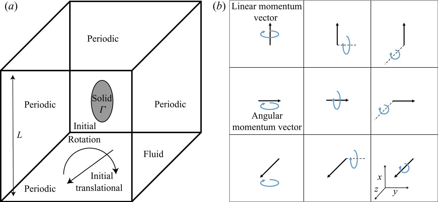
 $L \gg (a,b,c)$ as shown in figure 1. We define a density ratio
 $\rho =\rho _f/\rho _s$, where
 $\rho _f$ and
 $\rho _s$ are densities, and the subscripts
 $s$ and
 $f$ stand for solid and fluid, respectively. The kinetic energy of the solid is given by
 \begin{equation} K_s=\tfrac{1}{2} \left[{\boldsymbol{v}} \boldsymbol{\cdot} \mathcal{M}_s {\boldsymbol{v}} + {{\boldsymbol{\varOmega}} \boldsymbol{\cdot} \mathcal{I}_s {\boldsymbol{\varOmega}}}\right], \end{equation}
where  $\mathcal {M}_s$ is a diagonal
 $3\times 3$ matrix whose non-zero elements are the mass
 $m$ of the ellipsoid, while
 $\mathcal {I}_s$ is its moment of inertia tensor. Here,
 ${\boldsymbol {v}}$ is the translational velocity vector of the solid,
 ${\boldsymbol {\varOmega }}$ is its angular velocity vector and the superscript
 $\textrm {T}$ indicates the transpose. The fluid in the direct numerical simulations (DNS) is initially at rest, so
 $K_s$ comprises the total kinetic energy of the system. In an inviscid flow the kinetic energy is maintained constant through time, but gets interchanged between fluid and solid in interesting ways for a triaxial ellipsoid, as we shall see. Note that there is no gravity or any other body force in this problem. This enables the kinetic energy to be treated as the Hamiltonian of the system.
Problem definition.  $(a)$ A general ellipsoid with aspect ratio
 $a\,{:}\,b\,{:}\,c$ immersed in a fluid with initial energy ratio
 $E$, and
 $(b)$ schematic of nine initial conditions formed by basic configurations of the linear momentum and angular momentum vectors. The axes are defined as shown, in a frame of reference fixed with the body. A general initial condition can be constructed by a linear combination of these conditions.

We emphasise here the difference between a body held fixed, with a flow going past it, and one which is free to tumble and move. Auguste, Magnaudet & Fabre (Reference Auguste, Magnaudet and Fabre2013) have shown, for example, that the minimum Reynolds number for lateral motion in a freely falling thin disk is approximately half the Reynolds number at which a fixed disk would display wake instability. Although capable of far richer dynamics, there are far fewer studies on bodies free to move in fluids than those held fixed. It is hoped that the numerical method presented here will help to fill the gap, and enable viscous and inviscid studies on moving bodies. The code will soon be made publicly available.
In our DNS, the solid is subjected to an initial condition with a specified ratio,  $E$, of the initial translational kinetic energy,
 $k_t$, to the initial rotational kinetic energy,
 $k_r$, as follows:
 \begin{equation} E=\frac{k_t}{k_r}=\frac{m \left \| {\boldsymbol{v}} \right \|^2}{{\boldsymbol{\varOmega}} \boldsymbol{\cdot} \mathcal{I}_s {\boldsymbol{\varOmega}}}. \end{equation}
Once placed in an inviscid fluid,  $k_t$ and
 $k_r$ are the respective energies in fluid and solid together. Higher energy ratios indicate the dominance of initial translational kinetic energy over rotational. It is important to note that a range of initial conditions can be imposed for the same
 $E$, some basis combinations are shown in figure 1(b). We study immersed solids ranging from far heavier to much lighter than the fluid, and investigate their orbital behaviour under both inviscid and viscous conditions. In the viscous case, we define a particle Reynolds number,
 $Re_p = D_p U_0/\nu$, based on the solid length scale,
 $D_p$, and a fluid velocity-scale,
 $U_0$. In our simulations, we have chosen
 $D_p$ as the longest axis
 $a$ of the ellipsoid. We have developed an in-house solver, termed the Gerris immersed solid solver (GISS) (Shui et al. Reference Shui, Valluri, Popinet and Govindarajan2015) for our DNS. For solids immersed in inviscid fluids we cross-validate our DNS results against theoretical solutions of the Kirchhoff equations for inviscid fluids. Our DNS and theoretical methodologies are detailed in §§ 3 and 4.1, respectively.
3. DNS using GISS
The GISS numerical solver developed here comprises two subsolvers: (i) the Gerris flow solver; and (ii) the immersed solid solver. A two-step solution strategy is used. First, the three-dimensional (3-D) flow equations around the body are solved using the Gerris engine (Popinet Reference Popinet2003) to obtain velocity and pressure fields. These are then used to calculate the hydrodynamic force field on the surface of the immersed solid. Second, the calculated forces are passed on to the solid solver which calculates the new position of the immersed body using rigid body equations for translation and rotation. These steps allow for two-way solid–fluid coupling at every time step. The solver allows for arbitrary number of solids with arbitrary geometric features in six degrees of freedom (6DOF) motion. The solver can perform dynamical quad/octree mesh optimisation in a Cartesian framework, which greatly simplifies the procedure for mesh generation.
3.1. Fluid solver: governing equations and solution methodology
The fluid physics is solved using Gerris (Popinet Reference Popinet2003) which is based on a fractional-step projection method originally suggested by Chorin (Reference Chorin1967). We consider the fluid to be incompressible and Newtonian, and the immersed solid to be rigid and non-porous. Thus, the governing equations for the flow in the presence of such an immersed solid are
 \begin{gather} \boldsymbol{\nabla}\boldsymbol{\cdot}{\boldsymbol{u}} = 0, \end{gather}
 \begin{gather} \frac{\partial {\boldsymbol{u}}}{\partial t}+{\boldsymbol{u}}\boldsymbol{\cdot}\boldsymbol{\nabla}{\boldsymbol{u}} = -\frac{1}{\rho_f} \boldsymbol{\nabla} p + \nu\nabla^{2}{\boldsymbol{u}} + {\delta {\boldsymbol{f}_{\boldsymbol{S}}}}. \end{gather}
Here,  $\nu$ is the kinematic viscosity of the fluid. In our inviscid DNS we set
 $\nu =0$, which amounts to solving the Euler equations. Here,
 $p$ is the pressure,
 ${\boldsymbol {f}_{\boldsymbol {S}}}$ is a general body force characterising the influence of the immersed solid and
 $\delta =|\boldsymbol {\nabla } c|$ is the so-called interface delta function whose value is unity at the surface of the immersed body and zero elsewhere, with
 $c$ signifying the volume fraction of the fluid. Periodic boundary conditions are applied on the fluid domain and a no-slip non-penetration boundary condition is enforced on the immersed solid–fluid interface in viscous flow, thus,
 \begin{gather} {{\boldsymbol{u}}={\boldsymbol{u}}_{\varGamma}={\boldsymbol{v}} + {\boldsymbol{\varOmega}} \times ({\boldsymbol{r}}_M - {\boldsymbol{r}}_C)}, \end{gather}
 \begin{gather} \boldsymbol{\nabla} p \boldsymbol{\cdot} {\boldsymbol{n}}_{\varGamma} = 0. \end{gather}
Here,  $\varGamma$ indicates the immersed solid region and
 ${\boldsymbol {n}}_{\varGamma }$ indicates the normal to the solid. The projection method is based on Helmholtz–Hodge decomposition by which the velocity field
 ${\boldsymbol {u}}$ is uniquely decomposed into a solenoidal (divergence-free) part and an irrotational part. We rewrite the (3.1) and (3.2) in second-order, time-discrete semi-implicit forms, to get
 \begin{gather} \boldsymbol{\nabla}\boldsymbol{\cdot}{\boldsymbol{u}}^{n+1} = 0, \end{gather}
 \begin{gather} \frac{{\boldsymbol{u}}^{n+1}-{\boldsymbol{u}}^{n}}{\Delta t}+[({\boldsymbol{u}}\boldsymbol{\cdot}\boldsymbol{\nabla}){\boldsymbol{u}}]^n = -\frac{1}{\rho_f}\boldsymbol{\nabla} p^{n+1/2}+\nu\nabla^2 {\boldsymbol{u}}^n + {\delta {\boldsymbol{f}_{\boldsymbol{S}}}^n}. \end{gather}
Here, the superscript  $n$ denotes the variable at the time point of
 $t=n\Delta t$. (The coupling force,
 ${\boldsymbol {f}_{\boldsymbol {S}}}$, from the solid dynamics is treated in § 3.2.) With the help of an intermediate velocity field
 ${\boldsymbol {u}}^{\star }$, (3.6) can be divided into
 \begin{gather} \frac{{\boldsymbol{u}}^{\star}-{\boldsymbol{u}}^n}{\Delta t}+ [({\boldsymbol{u}}\boldsymbol{\cdot}\boldsymbol{\nabla}){\boldsymbol{u}}]^n = \nu\nabla^2 {\boldsymbol{u}}^n+{\delta {\boldsymbol{f}_{\boldsymbol{S}}}^n}, \end{gather}
 \begin{gather} \frac{{\boldsymbol{u}}^{n+1}-{\boldsymbol{u}}^{\star}}{\Delta t} = -\frac{1}{\rho_f}\boldsymbol{\nabla} p^{n+1/2}. \end{gather}
It is possible to calculate the value of  ${\boldsymbol {u}}^{\star }$ explicitly through (3.7) with the known velocity field
 ${\boldsymbol {u}}^n$, and with the help of (3.5), and by taking the divergence on both sides of the (3.8), we obtain
 \begin{equation} \nabla^2 p^{n+1/2} = \frac{\rho_f}{\Delta t} \boldsymbol{\nabla} \boldsymbol{\cdot} {\boldsymbol{u}}^{\star}. \end{equation}
Equation (3.9) is a typical Poisson equation, the solution of which will reveal the pressure field at the  $n+1/2$ time step. Substituting
 ${\boldsymbol {u}}^{\star }$ and
 $p^{n+1/2}$ back into (3.8), we then obtain the velocity field at the next time step as follows:
 \begin{equation} {\boldsymbol{u}}^{n+1}={\boldsymbol{u}}^{\star}-\frac{\Delta t}{\rho_f}\boldsymbol{\nabla} p^{n+1/2}. \end{equation}
3.2. Solid motion solver in GISS and coupling with fluid solver
At the outset, the reader is pointed to the extensive review by Wachs (Reference Wachs2019) on numerical techniques used for immersed non-spherical rigid bodies subject to various fluid environments. The methods used for GISS are similar to those mentioned in the references therein.
The governing equations for the solid are Newton's second law built on the global coordinate system which will remain stationary during the simulation. The solid is free to perform full 6DOF motion. While any number of solids can be immersed in the framework, computational effort rises with increasing number of solids. The calculation is powered by the open dynamics engine (known as ODE), developed by Smith (Reference Smith2005), which uses the following force and moment balance equations:
 \begin{gather} m\frac{{\boldsymbol{d}}{\boldsymbol{v}}}{{\boldsymbol{d}} t} = \iint_A \rho_f {\boldsymbol{f}_{\boldsymbol{S}}} \boldsymbol{\cdot} {\boldsymbol{r}}\,{\textrm{d}A}, \end{gather}
 \begin{gather} \mathcal{I}_s \frac{{\boldsymbol{d}} {\boldsymbol{\varOmega}}}{{\boldsymbol{d}} t} = {\iint_A ({\boldsymbol{r}}_M - {\boldsymbol{r}}_C) \times \rho_f {\boldsymbol{f}_{\boldsymbol{S}}}\,\textrm{d} A},\end{gather}
where  $V_s$ is the volume of the solid. Note that
 ${\boldsymbol {f}_{\boldsymbol {S}}}$ is the hydrodynamic force applied by the fluid on the solid–fluid interface (i.e. the solid surface). For any point on the surface of the solid,
 ${\boldsymbol {r}}$ is the relative location of that surface point to the mass centre of the solid,
 ${\boldsymbol {r}}_{\perp }$ is the positional vector of the surface point perpendicular to the axis of rotation of the solid,
 ${\boldsymbol {x}}$ is the instantaneous translational position of the centroid of the body and
 ${\boldsymbol {\alpha }}$ is the instantaneous set of Euler angles of the surface point with reference to the global coordinate system. Evidently,
 ${\boldsymbol {f}_{\boldsymbol {S}}}$ is a key coupling parameter between the flow and solid solvers. Equation (3.12) is built on a local coordinate system associated with the solid with the origin at its centre of mass and moves synchronously during the simulation. Though the orientation of the solid is represented by Eulerian angles at each time step, the internal calculations on the rotation are based on quaternions to avoid the so called Gimbal lock singularity (Kuipers Reference Kuipers1999). The conversion between them are as follows:
 \begin{gather} \left[\begin{array}{@{}c@{}}q_0\\q_1\\q_2\\q_3\end{array} \right]= \left[\begin{array}{@{}c@{}} \cos(\alpha_x/2)\cos(\alpha_y/2)\cos(\alpha_z/2)+\sin(\alpha_x/2)\sin(\alpha_y/2)\sin(\alpha_z/2)\\ \sin(\alpha_x/2)\cos(\alpha_y/2)\cos(\alpha_z/2)-\cos(\alpha_x/2)\sin(\alpha_y/2)\sin(\alpha_z/2)\\ \cos(\alpha_x/2)\sin(\alpha_y/2)\cos(\alpha_z/2)+\sin(\alpha_x/2)\cos(\alpha_y/2)\sin(\alpha_z/2)\\ \cos(\alpha_x/2)\cos(\alpha_y/2)\sin(\alpha_z/2)-\sin(\alpha_x/2)\sin(\alpha_y/2)\cos(\alpha_z/2)\end{array} \right], \end{gather}
 \begin{gather} \left[\begin{array}{@{}c@{}}\alpha_x\\\alpha_y\\\alpha_z\end{array} \right]= \left[\begin{array}{@{}c@{}} \mathrm{atan2}[2(q_0q_1+q_2q_3), 1-2(q_1^2+q_2^2)]\\ \mathrm{asin} [2(q_0q_2-q_3q_1)]\\ \mathrm{atan2}[2(q_0q_3+q_1q_2), 1-2(q_2^2+q3^2)]\end{array} \right]. \end{gather}
Here  $\alpha _i$ denotes the rotation angle around the
 $i$-axis of the instantaneous solid coordinate system and
 $q$ denotes the set of resulting quaternions.
On the boundary, the solid is represented by the volume fluid fraction,  $a$, and surface fluid fraction (
 $s_d$, where
 $d$ is the direction of the face) of the fluid together. Both
 $a$ and
 $s_d$ are set to the value of
 $1$ in pure fluid,
 $0$ in the pure solid, and any number between
 $0$ and
 $1$ means a mixed cell on the solid–fluid interface. This variant of immersed boundary method is usually referred as the ‘Cartesian grid method’ or the ‘embedded solid method’ (DeZeeuw & Powell Reference DeZeeuw and Powell1993; Udaykumar, Shyy & Rao Reference Udaykumar, Shyy and Rao1996).
To calculate the force applied on each cell, it is essential to know the area and direction of the interface which can be calculated approximately by
 \begin{equation} {\boldsymbol{A}}=(s_{x-}-s_{x+},s_{y-}-s_{y+},s_{z-}-s_{z+})\boldsymbol{\cdot}\Delta x^2. \end{equation}
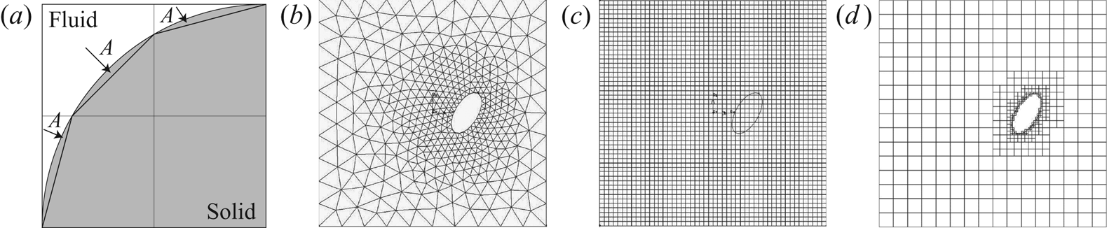
As shown by the example in figure 2, the area vector of the interface cutting the cell is  $(-1,-1)\boldsymbol{\cdot} \Delta x$,
 $|{\boldsymbol {A}}|$ is the area of the numerical interface with the direction of inward-pointing normal. Therefore, the body force tensor interpreted by the solid solver,
 ${\boldsymbol {F}}$ is
 \begin{align} {\boldsymbol{F}} &= \iint_A \rho_f {\boldsymbol{f}_{\boldsymbol{S}}} \boldsymbol{\cdot} {\boldsymbol{r}}\,{\textrm{d}A} \end{align}
 \begin{align} &=\left[A_x\enspace A_y \enspace A_z\right] \boldsymbol{\cdot} \mathcal{E}, \end{align}
where  $\mathcal {E} \equiv p - \mu (\boldsymbol {\nabla } u + \boldsymbol {\nabla } u^{\textrm {T}})$.
 $(a)$ Calculating surface area using fluid fraction and mesh refinement at fluid-interface elements.
 $(b)$ Typical dynamic mesh adaption,
 $(c)$ typical immersed boundary mesh,
 $(d)$ quadtree mesh in GISS.

The accuracy of  ${\boldsymbol {F}}$ improves with mesh refinement, as shown in figure 2. The Gerris fluid solver uses an adaptive mesh projection method (Popinet Reference Popinet2003). Mesh adaption is governed by a vorticity criterion,
 $\Delta x | \boldsymbol {\nabla } \times {\boldsymbol {u}} |/|{\boldsymbol {u}}_{max}| > \zeta$, where
 $\zeta$ is mesh tolerance. A unique feature in GISS is that the computational domain is discretised by a quadtree (two-dimensional (2-D)) or an octree (3-D) cell (cf. Samet Reference Samet1990; Ingram, Causon & Mingham Reference Ingram, Causon and Mingham2003). This allows GISS to exploit the advantages from both conventional dynamic mesh adaptation and immersed solid methods. A cell in the mesh will be automatically adapted by dividing the root cell to four (2-D) or eight (3-D) leaf cells under the criterion of vorticity, whilst all cells remain Cartesian. This ‘tree-structure adaptation’ of the mesh is simpler than the commonly used body-conformal unstructured mesh adaption (figure 2b–d).
For a mesh refinement level  $N$, the smallest mesh size,
 $\Delta x_{MIN}=L/2^N$ surrounds the solid. In dimensionless terms,
 $\Delta x^*_{MIN}=\Delta x_{MIN}/D_p$. We define mesh resolution as the inverse of mesh size, i.e.
 $R_m=1/\Delta x^*_{MIN}=D_p/\Delta x_{MIN}$. In order to ensure the continuity of numerical error between the fluid and the solid domains,
 $\Delta x^*_{MIN}|_{f}=\Delta x^*|_{s}$ where
 $\Delta x^*|_s$ is the mesh defining the immersed solid. This also ensures enforcement of the no-slip, no-penetration boundary condition on the walls of the solid. This also minimises error in calculation of the stress tensor around the solid and hence the drag and lift forces. During the simulation, the time step is set to fulfil both Courant and viscous criteria such that
 \begin{equation} \Delta t^* \leqq \min\left(\frac{\Delta x_{MIN}}{U_0}\frac{U_0}{D},\frac{\Delta x_{MIN}^2}{\nu}\frac{U_0}{D}\right) \implies \Delta t^* \leqq \min\left(\frac{1}{M_R},\frac{Re_p}{M_R^2}\right). \end{equation}
We can now apply Gauss's theorem on (3.9) and rewrite it in its spatial discrete equivalent with consideration of the fluid fraction
 \begin{gather} \iint_A \boldsymbol{\nabla} p \boldsymbol{\cdot} {\boldsymbol{n}}\, {\textrm{d}A}= \frac{\rho_f}{\Delta t}\iiint_V \boldsymbol{\nabla} \boldsymbol{\cdot} \boldsymbol{u}^{\star}\,{\textrm{d}V},\end{gather}
 \begin{gather} \sum_d s_d \boldsymbol{\nabla}_d p =\frac{\rho_f h c}{\Delta t} \boldsymbol{\nabla} \boldsymbol{\cdot} \boldsymbol{u}^{\star}. \end{gather}
Here,  $h$ is the local mesh size. Equation (3.20) is a general form of the Poisson equations solved by Gerris (Popinet Reference Popinet2003). We now perform some validation studies for the immersed solid solver.
3.3. Validating GISS for simple solid motion at finite Reynolds number
3.3.1. Bodies falling under gravity
The initial transient and the terminal velocity of a sphere settling in a fluid was validated against the experiments of Mordant & Pinton (Reference Mordant and Pinton2000) where beads were gently released in water, and against the theoretical calculations of Clift, Grace & Weber (Reference Clift, Grace and Weber1978). The experiments were simulated using a sufficiently spacious domain, to eliminate the effect of the side boundaries ( $L/D_p=32$). Our previous rigorous studies (Shui et al. Reference Shui, Valluri, Popinet and Govindarajan2015) suggested that a sixteenfold mesh refinement, defined as
 $R_m=1/16$, was dense enough around the body to accurately simulate settling.
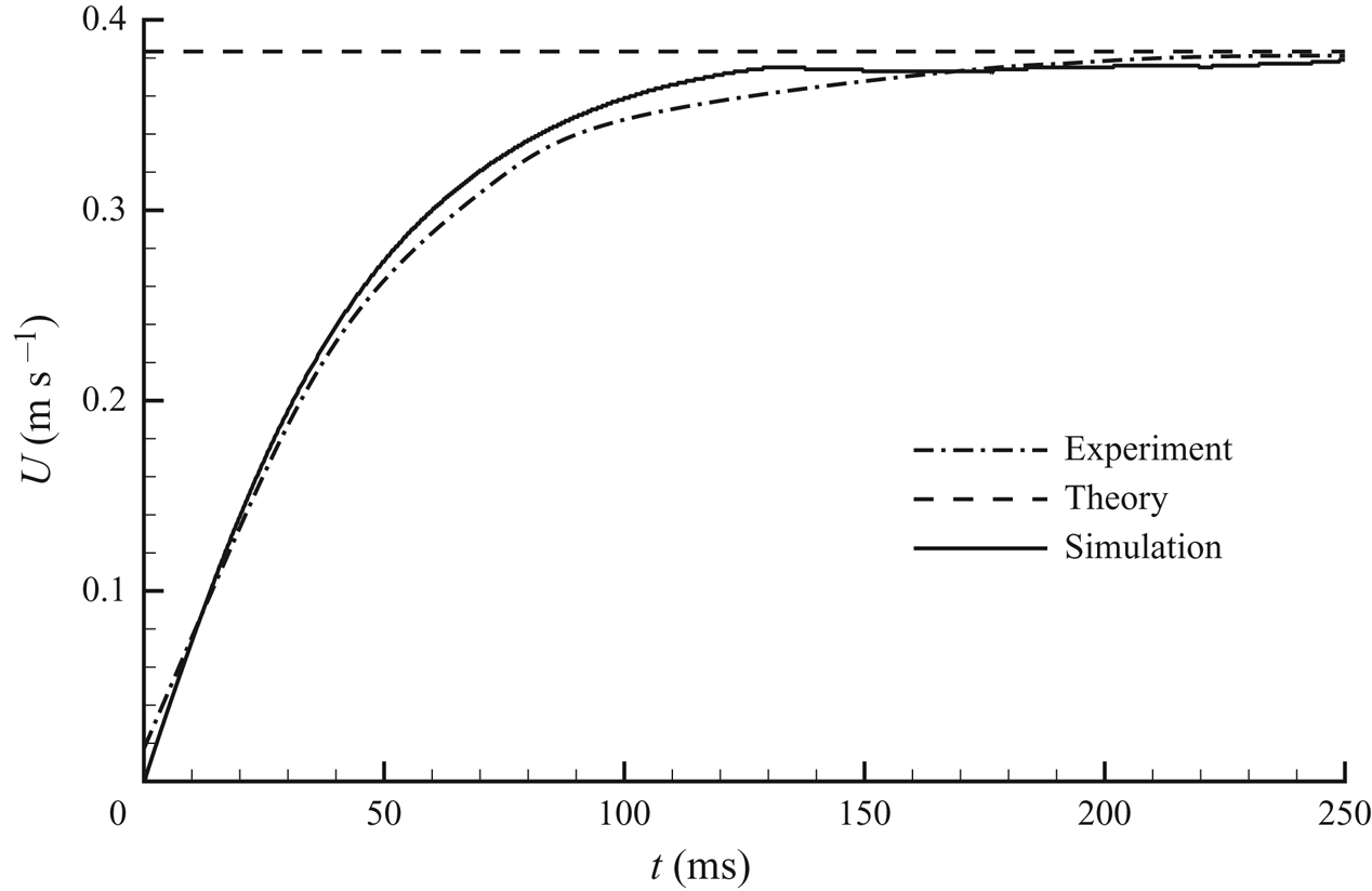
While we have simulated all the experimental cases of Mordant & Pinton (Reference Mordant and Pinton2000) in the range  $41 \le Re_p \le 430$, we present one of them in figure 3. The 3-D GISS solver shows good agreement with both the theoretical predictions for terminal velocity, and with experiments. The maximum relative error is around
 $2\,\%$ for the case of
 $Re_p=430$, similar to that of other cases. Our simulations show that the rotation of the solid is negligible (
 ${<}5^{\circ }$).
Settling of a sphere at  $Re_p=DU_0/\nu =430$, comparison against experiments of Mordant & Pinton (Reference Mordant and Pinton2000).

The solver was also compared against the work of Auguste et al. (Reference Auguste, Magnaudet and Fabre2013) concerning disks falling under gravity, see figure 4. We approximated the disk by a thin oblate spheroid and made two simulations at different Archimedes numbers and inertia ratios, defined by Auguste et al. (Reference Auguste, Magnaudet and Fabre2013), respectively, as  $Ar = (3|1-\rho |g a/16\rho )^{1/2}b/\nu$ and
 $I^*=\pi b/64 a \rho$, where
 $\rho$ is the fluid-to-solid density ratio,
 $g$ is acceleration due to gravity and
 $\nu$ is the kinematic viscosity of the surrounding fluid. In each case we found that a body starting from rest spontaneously exhibited the motion as described by them.
Falling styles of thin oblate spheroids  $(a = 1, \ b = 10, \ c = 10 )$ calculated by GISS corresponding to the work of Auguste et al. (Reference Auguste, Magnaudet and Fabre2013) on falling disks. (a) Autorotation trajectory observed at an Archimedes number of
 $Ar = 30$ and a dimensionless inertia ratio of
 $I^{*} = 3 \times 10^{-2}$ and (b) zigzag trajectory observed at
 $Ar = 40$ and
 $I^{*} = 2 \times 10^{-2}$. These behaviours agree with the regime plots presented in figure 2 of Auguste et al. (Reference Auguste, Magnaudet and Fabre2013).

3.3.2. Rotational motion describing Jeffery's orbits
In the Stokes limit of  $Re=0$, Jeffery (Reference Jeffery1922) analytically showed that a single neutrally buoyant ellipsoid in shear flow performs rotary motion. The orbit tracked is the so called Jeffery orbit. At low Reynolds numbers when the effects of inertia are negligible, the solution was confirmed in several experiments by Taylor (Reference Taylor1923).
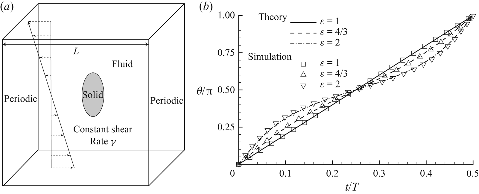
Here we validate the performance of GISS for the classical Jeffery orbit solution. Our set-up contains a neutrally buoyant spheroid subjected to Couette flow at constant shear rate,  $\xi$, in a channel. The channel is bounded by walls at the top and bottom, both moving with constant velocity but in opposite directions. The boundaries in the streamwise and spanwise directions are periodic, as shown in figure 5(a). The rotation of the solid is then compared against the theoretical result of Jeffery (Reference Jeffery1922).
Neutrally buoyant prolate spheroids executing classical Jeffery orbits.  $(a)$ Schematic.
 $(b)$ Angle versus time of spheroids of aspect ratio
 $\varepsilon$ stated in the legend, under shear flow defined by
 $Re_p=4 \xi a^2/\nu =0.1$. For comparison theoretical solutions are shown. Here
 $M=16$,
 $L^*=4$.

Figure 5(b) shows the rotation of prolate spheroids with different aspect ratio  $\varepsilon = a/b$. The angle and time shown are scaled by their values for one cycle. We may conclude that our simulated rotations are in very good agreement with theory (both spatially and temporally), thereby proving the ability of GISS to predict solid body rotation using the full Navier–Stokes equations at low
 $Re_p$. In figure 5 the Reynolds number based on the body's longest axis is
 $0.1$, and we have checked, using the theory of Einarsson et al. (Reference Einarsson, Candelier, Lundell, Angilella and Mehlig2015), that the finite Reynolds number corrections to Jeffery orbits for our biggest aspect ratio are three orders of magnitude smaller than the effects we retain. Note that only a sample from an exhaustive validation study available in Shui et al. (Reference Shui, Valluri, Popinet and Govindarajan2015) has been presented here.
Good agreement between the our DNS and earlier theory/experiments in the classical settling and rotation problems give us confidence in the ability of the GISS solver to tackle simple solid motion in viscous fluid. We now consider the more difficult case of an immersed solid in inviscid fluid presenting complex 6DOF motion.
4. Solid body immersed in an inviscid fluid
Under inviscid conditions this dynamics is described by the Kirchhoff equations. These are often termed the Kirchhoff–Clebsch equations, in recognition of the integrable cases found by Clebsch, and we refer to them most often by the latter name. These equations and our solutions are discussed below.
4.1. Kirchhoff–Clebsch equations and their solution
Provided that the ellipsoid is completely submerged by fluid which is inviscid, irrotational, incompressible and stationary at infinity, the fluid–solid system may be studied as a whole as follows, offering considerable simplification. The total kinetic energy,  $K_{tot}$, for the combined fluid–solid system may be written as
 \begin{equation} K_{tot}=\tfrac{1}{2}{\boldsymbol{v}} \boldsymbol{\cdot} \mathcal{M}{\boldsymbol{v}} + \tfrac{1}{2}{\boldsymbol{\varOmega}} \boldsymbol{\cdot}\mathcal{J}{\boldsymbol{\varOmega}}, \end{equation}
where
 \begin{equation} \mathcal{M} \equiv \mathcal{M}_f+\mathcal{M}_s, \quad \mathcal{J} \equiv \mathcal{I}_f+\mathcal{I}_s \quad \text{and} \quad \mathcal{A} =\begin{bmatrix} \mathcal{M}_f & \mathcal{S} \\ \mathcal{S}^{\textrm{T}} & \mathcal{I}_f \\ \end{bmatrix}. \end{equation}
Here,  $\mathcal {A}$ is the added mass tensor of the fluid, which includes both linear and rotational effects, and is dependent on the body shape and the fluid density. For anybody which is symmetric about three mutually perpendicular axes, we have a desirable simplification, in that
 $\mathcal {S}=0$, and further, for a triaxial ellipsoid,
 $\mathcal {M}_f$ and
 $\mathcal {I}_f$ are given in closed form (Lamb (Reference Lamb1945), see also Korotkin (Reference Korotkin2009)) by
 \begin{gather} \mathcal{M}_f = V_s \rho_f \begin{bmatrix} \dfrac{\alpha}{2-\alpha} & 0 & 0 \\ 0 & \dfrac{\beta}{2-\beta} & 0 \\ 0 & 0 & \dfrac{\gamma}{2-\gamma} \end{bmatrix}, \end{gather}
 \begin{gather} \mathcal{I}_f = \frac{V_s \rho_f }{5} \left[\begin{array}{@{}cc@{}} \dfrac{(b^2 - c^2)^2(\gamma - \beta)}{2(b^2-c^2)+(\beta-\gamma)(b^2+c^2)} & 0 \\ 0 & \dfrac{(a^2 - c^2)^2(\gamma - \alpha)}{2(a^2-c^2)+(\alpha-\gamma)(a^2+c^2)} \\ 0 & 0 \end{array}\right.\nonumber\\ \left.\begin{array}{c@{}} 0\\ 0\\ \dfrac{(a^2 - b^2)^2(\beta - \alpha)}{2(a^2-b^2)+(\alpha-\beta)(a^2+b^2)} \end{array}\right]. \end{gather}
In these expressions,
 \begin{equation} \alpha = abc \int_{0}^{\infty} \frac{d \lambda}{(a^2+\lambda)k_{\lambda}}, \quad \beta = abc \int_{0}^{\infty} \frac{d \lambda}{(b^2+\lambda) k_{\lambda}}, \quad \gamma = abc \int_{0}^{\infty} \frac{d \lambda}{(c^2+\lambda) k_{\lambda}}, \end{equation}
where
 \begin{equation} k_{\lambda}^2 = (a^2+\lambda) (b^2+\lambda) (c^2+\lambda). \end{equation}
The added mass terms are obtained by fourth-order Runge–Kutta integration of (4.5a–c), and the resolution is kept sufficient to obtain at least eight decimal place accuracy. In terms of the generalised momentum  ${\boldsymbol {P}} = (\mathcal {M}_f+\mathcal {M}_s){\boldsymbol {v}}$ and the generalised angular momentum
 $L = (\mathcal {I}_f+\mathcal {I}_s){\boldsymbol {\varOmega }}$ the Kirchhoff–Clebsch equations take the form (Aref & Jones Reference Aref and Jones1993)
 \begin{equation} \dot{{\boldsymbol{P}}} + {\boldsymbol{\varOmega}} \times {\boldsymbol{P}} = 0, \quad \dot{{\boldsymbol{L}}} + {\boldsymbol{\varOmega}} \times {\boldsymbol{L}} + {\boldsymbol{v}} \times {\boldsymbol{P}} = 0. \end{equation}
Our coordinate frame moves and is oriented with the body, and  ${\boldsymbol {v}}$ and
 ${\boldsymbol {\varOmega }}$ are its instantaneous velocity and angular velocity. This is a Hamiltonian system (Aref & Jones Reference Aref and Jones1993), where
 $-K_{tot}$ is the Hamiltonian. An examination of the Kirchhoff–Clebsch equations make it evident that there are two other integrals of the motion apart from
 $K_{tot}$, namely,
 ${\boldsymbol {P}} \boldsymbol {\cdot } {\boldsymbol {P}}$ and
 ${\boldsymbol {L}} \boldsymbol {\cdot } {\boldsymbol {P}}$. Solutions for the ordinary differential equations (4.7a,b) are obtained by a Runge–Kutta fourth-order scheme, and it is ensured that the three integrals of motion are maintained constant throughout the solution to at least six significant decimal places. The results of Aref & Jones (Reference Aref and Jones1993) were recovered excellently (not shown).
4.2. Symmetry and the limits of integrability
Equation (4.7a,b) represents a 6DOF system, and three integrals of the motion have been identified. Using the degeneracy properties of the relevant Poisson bracket, Kozlov & Onishchenko (Reference Kozlov and Onishchenko1982) were able to show, for a general ellipsoid, that if just one more integral of the motion is supported, the system is completely integrable. They did not obtain such an integral explicitly for any ellipsoid, but proved that the system is non-integrable when the ellipsoid's geometry satisfies the following condition:
 \begin{equation} j_a^{-1}(m_b-m_c) + j_b^{-1}(m_c-m_a) + j_c^{-1}(m_a-m_b) \ne 0, \end{equation}
where  $m_{a,b,c}$ and
 $j_{a,b,c}$ are the elements of the diagonal matrices
 $\mathcal {M}$ and
 $\mathcal {J}$ along the
 $a$,
 $b$ and
 $c$ semiaxes of the ellipsoid. We notice immediately that if the ellipsoid has an axis of rotation, namely two of the axes, say
 $b$ and
 $c$ are equal, then
 $j_b=j_c$ and
 $m_b=m_c$, and it is trivial to see that the above inequality is never satisfied, i.e. the dynamics is integrable. Several authors, such as Holmes, Jenkins & Leonard (Reference Holmes, Jenkins and Leonard1998) and Dragović & Gajić (Reference Dragović and Gajić2012) have identified this property. Such ellipsoids are referred to as ellipsoids of revolution, or as prolate spheroids where
 $a>b$ and oblate spheroids where
 $a<b$. The system must exhibit periodic or quasiperiodic behaviour in this case. The dynamics of such a body of revolution, if there is no surrounding fluid, reduces to the Lagrange case of a symmetric top (Landau & Lifshitz Reference Landau and Lifshitz1969). In the general case of a triaxial ellipsoid, which we define as one where
 $a \neq b \neq c$, our numerical search revealed, as we expected, no ratio of semiaxes where (4.8) was violated. So for practically any triaxial ellipsoid, the dynamics is non-integrable, and we should be able to obtain chaotic trajectories in at least some part of the phase space. Aref & Jones (Reference Aref and Jones1993) identified one such ellipsoid as satisfying the above condition, with semiaxes in the ratio
 $1.0$,
 $0.8$ and
 $0.6$, and demonstrated the existence of chaotic trajectories.
For a sphere,  $\alpha =\beta =\gamma =1/2$, we recover its well known added mass. Moreover,
 $\mathcal {I}_f$ in this case is just
 $0$, so a sphere will not be rotated by an inviscid fluid. We thus have
 $\dot {{\boldsymbol {L}}}=0$, with which the conditions for integrability are trivially satisfied. For a spheroid, we explicitly identify another integral of the motion below, and show physically how it considerably simplifies the dynamics.
4.3. Validating our numerical approach for 6DOF motion in inviscid environments
The Kirchhoff–Clebsch system, being inviscid, and in addition offering a rich tapestry of complex behaviour, provides a rigorous benchmark for validating any numerical approach. Our inviscid direct numerical simulation is set up as shown in figure 1(a). The domain size is  $L=512a$ where
 $2a$ is the major axis of the ellipsoid. All sides of the domain are periodic. Such a large domain is chosen to ensure that the solid has enough space to track chaotic orbits without interference from residual wakes (in the viscous case) due to the periodic boundary conditions. The highest mesh resolution was set as
 $128$ grid points on the solid surface, and adaptive mesh refinement ensures that the flow around it is adequately resolved. The ellipsoid is given an initial velocity
 $U_0$ and angular velocity
 $\varOmega _0$ which are perpendicular to each other and shown in some of the schematics in figure 1(b). Note that the dot product of the momentum and angular momentum in this case is zero, and, since it is an integral of the motion, will remain zero throughout the simulation. We recommend this, to reduce the time needed for the ellipsoid to explore a statistically significant region of the system's phase space, but any angle between the two may be used, and will not change the results qualitatively, as we have shown above. In our Kirchhoff–Clebsch solutions we have used a far wider range of initial conditions as will be discussed below. We wish to obtain the trajectory executed by a marker point,
 $M$, located on the surface of the ellipsoid. The relative location of
 $M$ is
 \begin{equation} {\boldsymbol{r}}_M={\boldsymbol{x}}_M-{\boldsymbol{x}}_C, \end{equation}
where  ${\boldsymbol {x}}_M$ is the positional vector of
 $M$ in the global frame and
 ${\boldsymbol {x}}_C$ is the positional vector of the solid centre in the global frame. Hence, plotting
 ${\boldsymbol {x}}_C$ shows the trajectory of the solid centre moving in the fluid, and plotting
 $\boldsymbol {{\boldsymbol {r}}_M}$ shows the orbit of the marker point relative to the solid centre itself, representing the orientation of the solid. These vectors as solutions of the equations, give an immediate view of how the orientation and position of the ellipsoid changes as it moves through the fluid.
4.3.1. Periodic and quasiperiodic dynamics
We consider an ellipsoid of revolution, with  $a\,{:}\,b\,{:}\,c=1\,{:}\,0.7\,{:}\,0.7$. The initial energy ratio is specified as
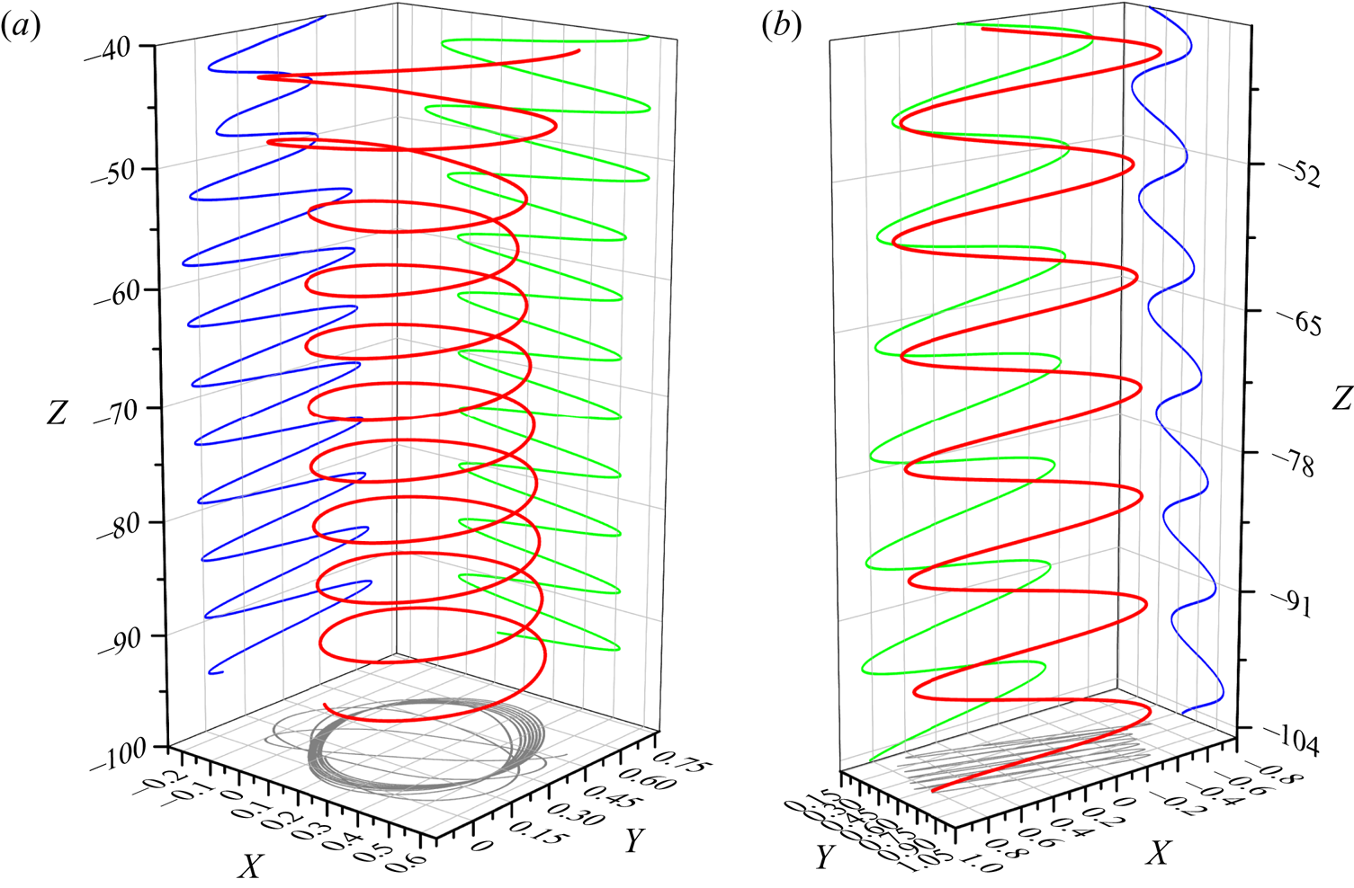
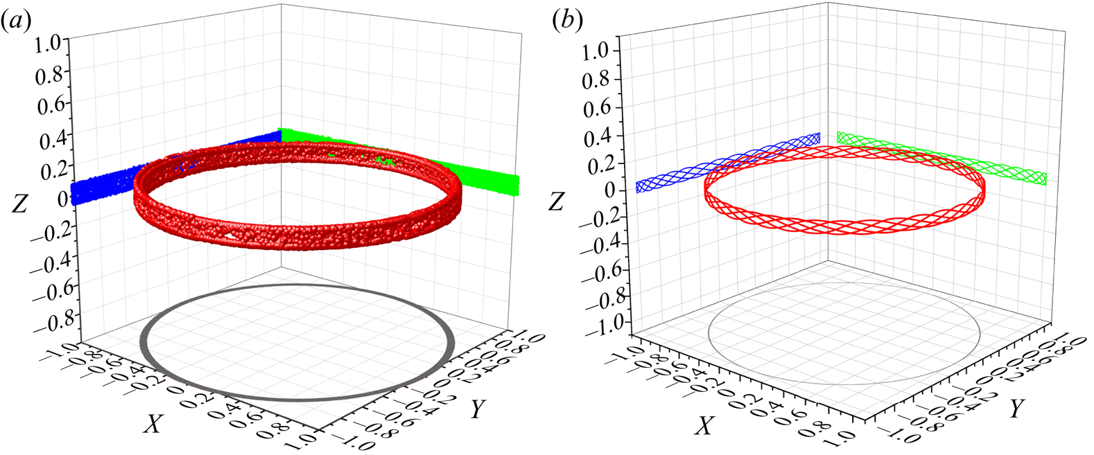
 $E=1$. Figure 6(a) shows an orbit described by the marker point,
 ${\boldsymbol {r}}_M$, about the centre of mass of the ellipsoid using GISS simulations. It is seen that
 ${\boldsymbol {r}}_M$ describes a near-circular orbit in the
 $x$–
 $y$ plane. Every time the orbit is described, the location on the
 $z$-axis is slightly different, and we cannot yet distinguish whether this is due to numerical errors or due to the quasiperiodic nature of the orbit. We shall return to this point below. It is obvious, however, that the dynamics is not chaotic. This conclusion agrees well with our own solution of the Kirchhoff–Clebsch equations, example shown in figure 6(b). The initial conditions are the same in both the cases.
Periodic orbits tracked by a marker point  $M$ on an ellipsoid of revolution with
 $a\,{:}\,b\,{:}\,c=1\,{:}\,0.7\,{:}\,0.7$ at
 $E=1$ and
 $\rho = 1$. The orbit (locus of points defined by
 ${\boldsymbol {r}}_M$) is represented in red, with its projections on the
 $XY$,
 $XZ$ and
 $YZ$ planes in grey, blue and green, respectively. The initial conditions are the same in both solutions.
 $(a)$ Inviscid DNS solution.
 $(b)$ Kirchhoff–Clebsch solution.

4.3.2. Chaotic dynamics
We next study the dynamics of a triaxial ellipsoid, with  $a\,{:}\,b\,{:}\,c=1\,{:}\,0.8\,{:}\,0.6$. This was the shape studied by Aref & Jones (Reference Aref and Jones1993) whose sample result indicated that increasing the ratio
 $\rho$ of fluid density to solid density increases the propensity for chaotic orbits.
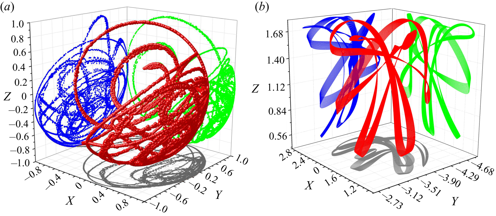
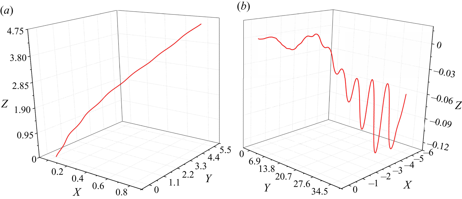
The initial condition is quantified at  $E=20$. Figure 7(a) shows clearly that the orbit tracked by the marker point using GISS simulations is chaotic. This also agrees well with our own solution of the Kirchhoff–Clebsch equations, shown in figure 7(b). Apart from the marker point it is instructive to obtain the trajectories tracked by the centroids
 ${\boldsymbol {x}}_C$ of the periodic and chaotic ellipsoids in DNS. These are shown in figure 8(b). After an initial transient during which the fluid gains kinetic energy, the centroid of the ellipsoid of rotation settles into motion on a line, and we have seen earlier that it is in steady rotation about its centroid. The triaxial ellipsoid on the other hand executes irregular motion.
Chaotic orbits tracked by a marker point  $M$ on a triaxial ellipsoid
 $a\,{:}\,b\,{:}\,c=1\,{:}\,0.8\,{:}\,0.6$ at
 $E=20$ and
 $\rho = 1$. The initial conditions are the same in both solutions.
 $(a)$ Inviscid DNS solution.
 $(b)$ Kirchhoff–Clebsch solution.

Trajectories of the centroids of the ellipsoids (locus of points defined by  ${\boldsymbol {x}}_C$) for
 $(a)$ the simulation of the ellipsoid of revolution shown in figure 6(a), and
 $(b)$ that of the triaxial ellipsoid of figure 7(a). These are results from inviscid DNS.
 $(a)$ Periodic system.
 $(b)$ Chaotic system.

Thus our numerical approach not only works well in inviscid environments as well, but is able to demonstrate the Kozlov–Onishchenko theorem by showing chaotic trajectories in the case of a triaxial ellipsoid, and a reduction to simple dynamics for an ellipsoid of revolution. We next present a method to quantify orbital behaviour.
4.4. Understanding orbital behaviour using RQA
We use RQA to quantify orbits tracked by solid bodies. A recurrence plot (RP) is the foundation of RQA. Eckmann et al. (Reference Eckmann, Oliffson Kamphorst and Ruelle1987) introduced RPs, as a way to visualise the dynamics of a system through its phase space, marking all time points when a said event recurs. The main advantage of RPs is that they provide a means to investigate behaviour of N-dimensional dynamics using a 2-D plot. Recurrence is defined by (4.10) as follows:
 \begin{equation} R(i,j)=\begin{cases}1 & \text{if}\ \|{\boldsymbol{x}}_M(i) -{\boldsymbol{x}}_M(\,j)\|_{\infty} \leq \epsilon,\\ 0 & \text{otherwise}, \end{cases} \end{equation}
where  $R(i,j)$ is an N-by-N matrix,
 $N$ being the number of samples in the time series,
 ${\boldsymbol {x}}_M(i)$ is the position of the marker point M in the phase space of the body at time
 $i$ and
 ${\boldsymbol {x}}_M(\,j)$ is the position of the marker point in the phase space of the body at time
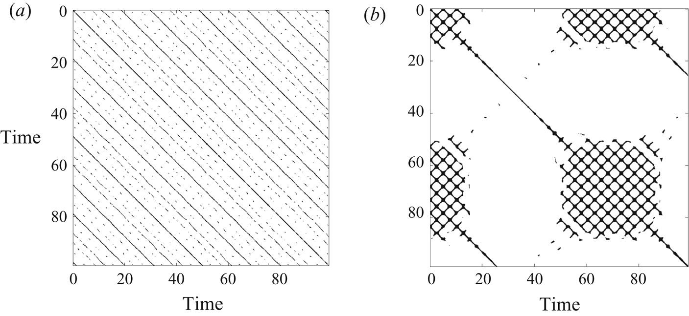
 $j$. A thought experiment will tell us that a perfectly periodic system will only have solid diagonal lines in the RP, and the spacing of the diagonal lines will be periodic. A quasiperiodic system will have only diagonal lines, but these could be broken into segments. Deterministic chaos of a small number of degrees of freedom presents visually interesting patterns in the RP. On the other hand, white noise would display an RP composed of randomly spaced single dots. At a given time
 $j$, our RQA steps through the array
 $i$ to check for recurrence of the position of the marker point for each time step. In the case of our solution of the Kirchhoff–Clebsch equations, we use approximately 100 000 time steps and in our DNS it is approximately 200 000 time steps, with each time step recording the spatial location of the marker point. Since perfect recurrence is nearly impossible due to numerical noise,
 $\epsilon$ is the heuristic threshold distance which determines where two given states are sufficiently close to count as a recurrence. In this work, we set
 $\epsilon =5\,\%$ of the maximum phase-space diameter, i.e. the maximum displacement presented by the solid in any simulation, in line with the recommendations of Marwan (Reference Marwan2008). We make use of three statistical measures to quantify chaos, as defined below.
We define  $RR$ as the recurrence rate of the system, representing the probability of the solid's orientation to recur in the orbit as follows:
 \begin{equation} RR=\frac{1}{N^2} \sum_{i,j=1}^N R(i,j). \end{equation}
We next define  $DET$ as the determinism exhibited by the system, which is a measure of the predictability of any dynamical system, as follows:
 \begin{equation} DET=\frac{\sum_{\ell=\ell_{min}}^N\ell P(\ell)}{\sum_{i,j=1}^N R(i,j)}, \end{equation}
where  $P(\ell )$ is the frequency distribution of the lengths of the diagonal lines in a recurrence plot,
 $\ell$ is the length of those lines and
 $\ell _{min}$ is the criterion used to indicate the presence of a line. This is set to
 $2$ in our work, which means that a minimum of two points (pixels) are needed to lay diagonally next to each other. We also define
 \begin{equation} p(\ell) = \frac{P(\ell)}{\sum_{\ell=\ell_{min}}^N P(\ell)}, \end{equation}
as the probability of a diagonal line giving exactly length  $\ell$. The Shannon entropy,
 $ENTR$, of the RP, given by
 \begin{equation} ENTR =-\sum_{\ell=\ell_{min}}^N p(\ell) \ln(p(\ell)), \end{equation}
can be calculated by this distribution. The entropy corresponds to the complexity of the deterministic structure in the system (Marwan et al. Reference Marwan, Carmen Romano, Thiel and Kurths2007).
These statistics can be made time-dependent through computing over small time windows. The windows can be moved over the RP along the line of identity. These time-dependent measures can be useful to detect periodic–chaos regime transitions (Marwan Reference Marwan2008). We define a moving time window,  $t_w$, over simulation time. Thus the number of simulation time steps within the prescribed window is
 \begin{equation} N_w=\frac{t_w}{\Delta t}, \end{equation}
where  $\Delta t$ is the simulation time step size. Using such a moving window, we can then compute the RQA statistics at any time
 $t$, corresponding to a time step
 $n = t/\Delta t$ as
 \begin{gather} RR(t) =\frac{1}{{N_{w}}^{2}}\sum_{i,j=n}^{N_{w}} R(i,j), \quad DET(t)=\frac{\sum_{\ell=\ell_{min}}^{N_{w}} \ell P_{t,t_{w}}(\ell)}{\sum_{i,j=n}^{N_{w}} R(i,j)}, \end{gather}
 \begin{gather} p_{t}(\ell) = \frac{P_{t,t_{w}}(\ell)}{\sum_{\ell=\ell_{min}}^{N_{w}} P_{t,t_{w}}(\ell)}, \quad ENTR(t) =-\sum_{\ell=\ell_{min}}^{N_{w}} p_{t}(\ell) \ln(p_{t}(\ell)). \end{gather}
Here,  $P_{t,t_{w}}(\ell )$ is the instantaneous frequency distribution of the lengths of the diagonal lines in an RP with respect to a window size of
 $t_w$, and
 $p_{t}(\ell )$ is the instantaneous probability of a diagonal line giving exactly length
 $\ell$ calculated over a moving time window
 $t_w$. In order to quantify which case is chaotic,
 $DET$ is a very useful metric, (Eckmann et al. Reference Eckmann, Oliffson Kamphorst and Ruelle1987). As can be seen in (4.12), it is a measure of the fraction of points in the RP that form diagonal lines. A purely stochastic system would have a recurrent plot comprising scattered points, whereas a periodic or quasiperiodic system shows long running diagonal lines (Marwan Reference Marwan2008).
We identify orbital behaviour based on the RPs and time dependent RQA statistics. Since periodic and quasiperiodic behaviour will consist only of diagonal lines or line segments, if we choose an  $N_w$ long enough to cover an orbital time,
 $RR$ will remain constant, and
 $DET$ will stay at a value of
 $1$. On the other hand
 $RR$ will not be constant, and
 $DET$ must be less than
 $1$ in a chaotic system. Similarly, the entropy remains constant in a periodic or quasiperiodic system but varies with time in a chaotic system. Features in these statistics can reveal further information about the behaviour of the system.
Figure 9 shows RPs corresponding to the non-chaotic orbital behaviour corresponding to the parameters used in figure 6, and chaotic orbital behaviour of the case in figure 7. In figure 9(a), the fact that the diagonal lines are often broken is indicative of quasiperiodic rather than strictly periodic motion of the marker point; similar patterns for quasiperiodic systems has been studied by Marwan et al. (Reference Marwan, Carmen Romano, Thiel and Kurths2007). Whereas, in the case of chaotic orbital motion, figure 9(b) demonstrates a complex structure indicating irregular and unpredictable recurrence. At first sight the recurrence rate pattern seems to repeat itself in a regular manner. We recall that the high departure from a diagonal structure is already indicative of strongly chaotic dynamics. But we further ensured that there is no periodic pattern in the recurrence rate plot as well, by generating a residual RP by taking the difference between the original recurrence time series and a time-shifted copy. The time shift was selected to minimise the error between the two series, and it was obvious that there was no overlap (not shown).
Recurrence plots,  $(a)$ parameters as in figure 6. The regular diagonal bands are a signature of non-chaotic behaviour; and
 $(b)$ chaotic system, case as in figure 7. The complex structures are signature of chaotic behaviour. These results were produced by solving the Kirchhoff–Clebsch equations.

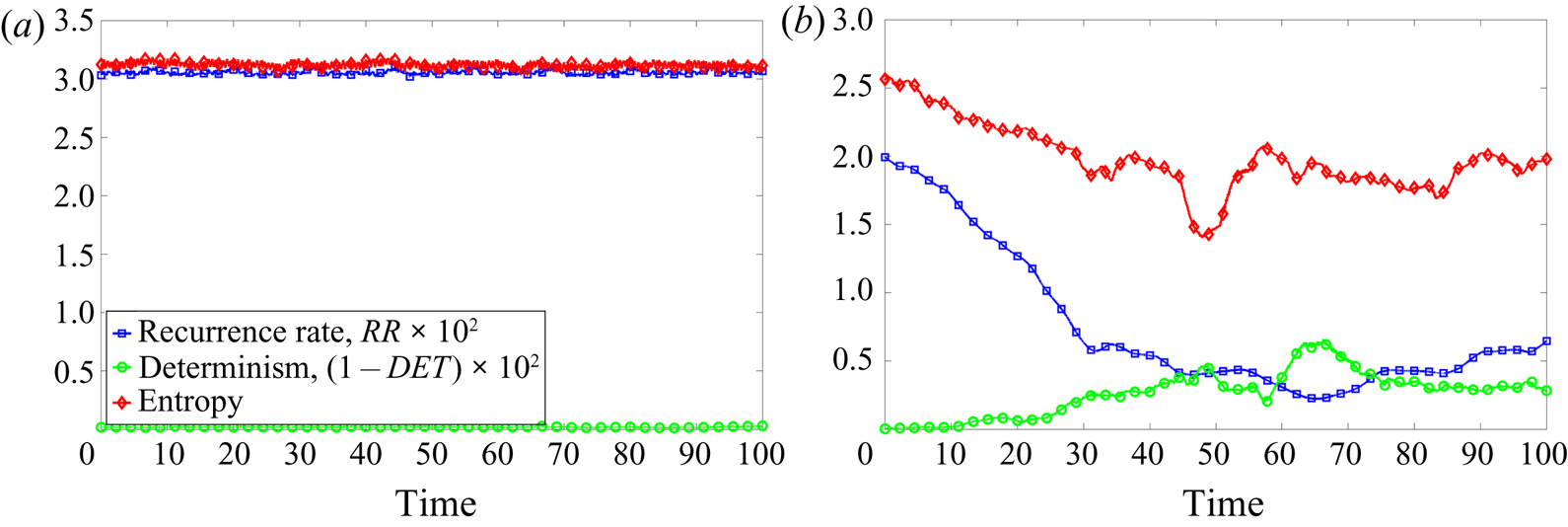
Figure 10 shows the behaviour of key statistical parameters,  $RR$,
 $DET$ and
 $ENTR$, over the period of the simulations to quantify orbital behaviour. For a periodic system, as shown in figure 10(a), these statistics remain largely constant, and the
 $DET$ is 1 (or,
 $\hbox{1-DET=0}$). Whereas in a chaotic system, figure 10(b) demonstrates that none of these parameters remain constant, and
 $DET<1$. These statistics along with the texture of the RP are used to classify the behaviour of the orbits generated later in the paper. We will also use Poincare sections to distinguish chaotic from non-chaotic behaviour.


5. Dynamics in an inviscid environment
There are four non-dimensional parameters in the inviscid problem: the axis ratios  $b/a$ and
 $c/a$, the fluid-to-solid density ratio
 $\rho$ and the ratio
 $E$ of the initial kinetic energy of the system in rotational motion to that in linear motion of the body centroid.
To address the effect of the axis ratios we first ask what it is about a triaxial ellipsoid that makes it possible to see chaos in its dynamics and not in a spheroid. We answer that the added mass enables it. The primary difference between a spheroid and a triaxial ellipsoid is in the added complexity of the added mass tensor of the latter. In the case of a spheroid, two entries each of  $\mathcal {M}$ and
 $\mathcal {J}$ in (4.2a–c) become equal to each other, so the added mass tensor
 $\mathcal {A}$ has only four independent entries rather than six as in a triaxial ellipsoid. With some algebra we show that a spheroid as a result has an additional integral of the motion:
 $l_1$, the angular momentum component along the
 $x$-axis. Our explicit identification of this integral of the motion helps obtain a physical understanding of how a spheroid can only display limited dynamics. The integral means the rate of rotation about the unequal axis, i.e. the long axis of a prolate spheroid or the short axis of an oblate spheroid, remains constant. So all changes in the angular momentum of the system are restricted to the plane perpendicular to the
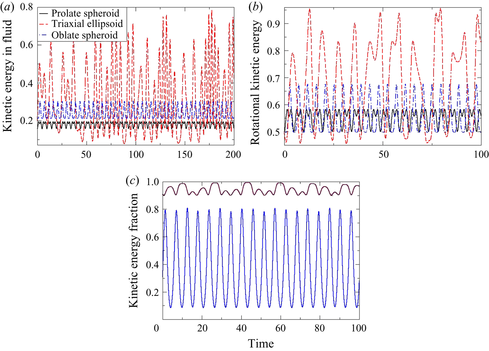
 $x$-axis. This, as we shall see, will be an important factor for determining the dynamics of spheroids in viscous fluids as well. We ask if a triaxial ellipsoid can therefore exchange kinetic energy more freely with the surrounding fluid than a spheroid can. Figure 11(a) shows what fraction of the total kinetic energy at a given time is in the fluid. (The kinetic energy fraction in the solid is just this quantity subtracted from
 $1$.) All conditions except the ratio of the axes are kept the same across the curves. This figure is just one example of a whole range of computations we have made, which give the same qualitative behaviour. Apart from varying
 $\rho$ and
 $E$ we have used many different orientations between the solid and its linear momentum, and between the linear and angular momenta. We thus show that the dynamics of the prolate and the oblate spheroids are limited, in that they only interact through minor exchanges of the kinetic energy between solid and fluid. The triaxial ellipsoid, however, wildly exchanges kinetic energy between solid and fluid. It is intuitive that this possibility of exchange provides for a rich range of tumbling dynamics. We digress briefly here to emphasise that added mass effects are of irrotational origin, and we therefore expect a triaxial ellipsoid to behave differently in a qualitative way in viscous flow as well as compared to a spheroid. Moreover, the added mass provides for an exchange of kinetic energy between motion of the centroid and that contained in tumbling. This exchange is shown terms of the fraction of total kinetic energy in rotational motion in figure 11(b). Here,
 $E=1$ implies that the initial fraction in rotation is
 $0.5$. Again we see that the fraction in rotational motion changes by a large amount in the case of the triaxial ellipsoid whereas the spheroids retain a ratio close to their starting value. We are able to get cases in the triaxial ellipsoid where the rotational energy goes from very low to high values, thus executing a complicated self-generated run-and-tumble dance.
 $(a)$ Fraction of kinetic energy in the fluid as a function of time for a triaxial ellipsoid, as compared to prolate and oblate spheroids of the same volume. These are solutions of the Kirchhoff–Clebsch equations, with
 $\rho =1$ and
 $E=1$. The energy exchange between fluid and solid is much larger in a triaxial ellipsoid. For clarity of viewing the curve for the oblate spheroid is displaced by
 $0.05$ in the vertical.
 $(b)$ Fraction of kinetic energy in rotational motion as a function of time in the same run (and legend) as in panel
 $(a)$.
 $(c)$ The triaxial ellipsoid in periodic motion,
 $\rho =0.1$,
 $E=1$. The plot shows the fraction of kinetic energy as a function of time in the fluid (blue solid line) and the fraction of kinetic energy in rotational motion (purple long-dashed line).

Any chaotic system must have periodic windows in state space, so we must have initial conditions giving rise to periodic motion. For one such condition for the triaxial ellipsoid, we plot in figure 11(c) the ratios of kinetic energy in the fluid as opposed to the solid, and in rotational as opposed to translational motion. While the solid remains primarily in rotational motion, the sharing between fluid and solid varies across most of the available range. This was never seen in the spheroid in all our attempts. Thus, even for periodic motion, more variety in dynamics is attainable with the triaxial ellipsoid than with spheroids.
This brings us to an important question. What fraction of phase space is chaos seen in (or, given that this is a Hamiltonian system, what fraction of tori are disintegrated) and does this, for a given body shape, depend on  $\rho$ and
 $E$? We find that there are two limiting cases, where the motion cannot be chaotic even in a triaxial ellipsoid. When the fluid-to-solid density ratio is
 $0$, the added mass of the fluid is zero. In this case,
 ${\boldsymbol {P}}$ and
 ${\boldsymbol {v}}$ are collinear, and by some algebra we show that
 ${\boldsymbol {\varOmega }} \boldsymbol {\cdot } {\boldsymbol {L}}$ is an additional integral of the motion, which is another way of saying that rotational and translational kinetic energies are not exchanged. So the motion becomes integrable. In other words, the Kozlov–Onishchenko theorem is applicable when there is added mass in the system. In fact at zero fluid density, namely in vacuum, the dynamics reduces to periodic behaviour. The ‘asymmetrical top’ of which a triaxial ellipsoid is an example (Landau & Lifshitz Reference Landau and Lifshitz1969), displays an instability when spun around its intermediate axis, going into a 3-D tumbling state, but remaining periodic. Secondly, when the initial linear momentum is zero, i.e. the body initially is only in rotational motion, or
 $E=0$, the first of the Kirchhoff–Clebsch equations is identically zero, and the motion reduces to one of constant rotation. We realise from the Kozlov–Onishchenko theorem that for all other
 $\rho$ and
 $E$, there will be some region of phase space where there is chaos. For a range of these parameters over several orders of magnitude, we estimate where the probability of attaining chaotic dynamics from a randomly chosen set of initial conditions is higher than half. For this we ensure that the initial phase space conditions are uniformly sampled, and perform simulations for 20 or more initial conditions at each
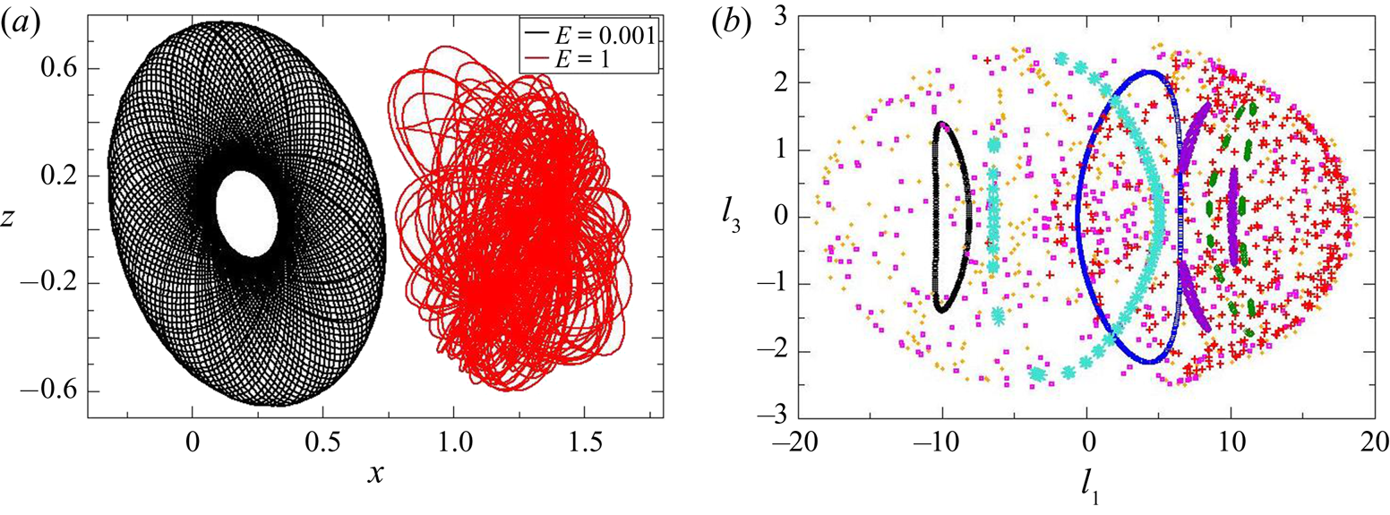
 $(\rho ,E)$. Chaotic behaviour may be easily distinguished from periodic or quasiperiodic behaviour visually by examining the trajectory of the marker point, and an appealing example of a triaxial ellipsoid's tip covering a doughnut in quasiperiodic motion is shown in figure 12(a) in contrast to a chaotic orbit. The fastest way to make this distinction for a large number of initial conditions is to obtain Poincare sections, such as shown in figure 12(b). The section chosen here is when
 $p_2$, the
 $y$-component of the linear momentum,
 ${\boldsymbol {P}}$ goes through a
 $0$ while decreasing, and the plane shows the
 $x$- and
 $z$-components of the angular momentum
 ${\boldsymbol {L}}$. Each colour and symbol here is the Poincare section corresponding to a different initial condition, with all non-dimensional parameters in the problem kept constant. Quasiperiodic orbits appear as single closed orbits (e.g. the black and blue symbols) or multiple closed orbits (e.g. the purple and green symbols) whereas chaotic orbits appear as scattered points on the plane. The parameters
 $E$ and
 $\rho$ are such that we are close to the border between predominantly chaotic and predominantly periodic behaviour, so depending on where in the sample space our initial condition lies, we can get both types of behaviour.
Distinguishing chaotic dynamics from quasiperiodic.  $(a)$ Typical motion of the marker point relative to the centre of mass of the body in quasiperiodic (
 $E=0.001$) and chaotic (
 $E=1$) dynamics. Here
 $\rho =1$. The view shown is in the
 $x$–
 $z$ plane. The chaotic trajectory has been shifted on the
 $x$-axis by
 $1.1$ for clearer viewing.
 $(b)$ Typical Poincare section showing components of the angular momentum
 $l_3$ versus
 $l_1$ at the time when the linear momentum component
 $p_3$ goes through a zero while decreasing. Each colour or symbol stands for a different initial condition. Here
 $E=10$ and
 $\rho =0.1$. These are solutions of the Kirchhoff–Clebsch equations.

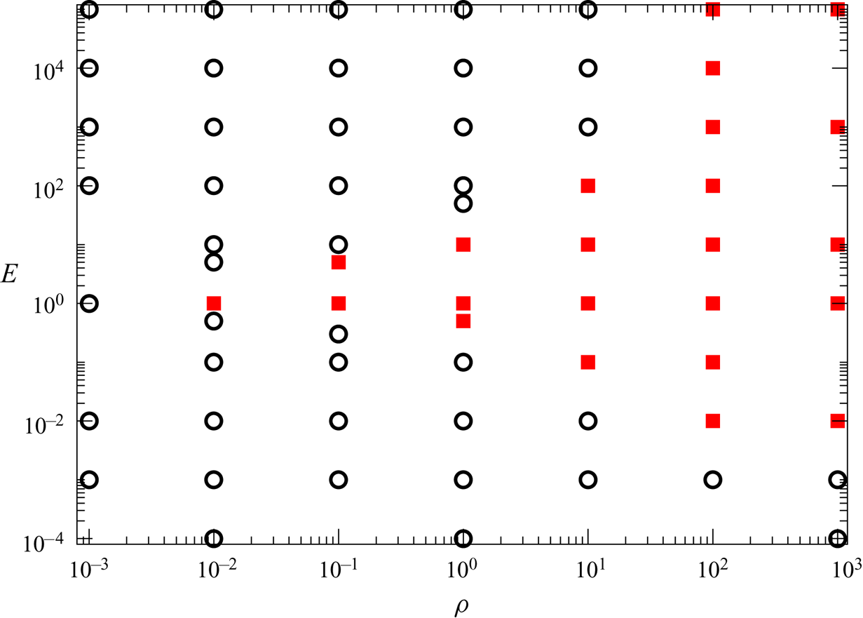
The boundary between a majority periodic state space and majority chaotic is shown in figure 13. By repeating the exercise close to the boundary points, we find that the results are robust. However, we hasten to add that these are conclusions from a randomly sampled set of the phase space. As we move away from the boundary, the propensity for chaotic behaviour becomes predominant in the regime covered by the red squares in the figure, while periodic or quasiperiodic behaviour occurs with high probability in the black circled regime. Given our arguments for zero fluid density, and the importance of added mass for chaotic dynamics, it is intuitive that the propensity for chaos should increase with increasing fluid density. This is evident from the figure. So a body in a very light fluid, while technically in non-integrable motion, is very unlikely to display chaos. At the right of the figure, the solid density approaches zero, we have a bubble in the shape of a triaxial ellipsoid in an inviscid fluid. The added mass dominates the dynamics, and the system is almost always chaotic. We discussed earlier how  $E=0$ could never result in chaotic motion, and this propensity continues into small values of
 $E$ for any density ratio. So in a fluid of any density, we see a triaxial ellipsoid will not display chaos if it was initially in predominantly rotational motion. We further see that at
 $E \sim 1$, where rotational and translational motion have comparable energy initially, is most conducive for chaotic motion, and under such initial conditions, the ellipsoid is wont to display chaotic motion even if it is a hundred times more dense than the fluid. At high values of initial linear momentum, while there is the possibility offered by the Kirchhoff–Clebsch system for converting translational to rotational motion, the system, at moderate fluid densities tend towards periodic dynamics, but at higher fluid densities displays chaos. We created an analogous figure (not shown) where we used the total kinetic energy rather than the ratio
 $E$ as our parameter, and found that there was no simple boundary between chaotic and non-chaotic motion. So
 $E$ is a physically appropriate choice.
Orbital behaviour map of an ellipsoid with aspect ratio  $a\,{:}\,b\,{:}\,c=1\,{:}\,0.8\,{:}\,0.6$ submerged in an inviscid environment (solutions of the Kirchhoff–Clebsch equations). At least twenty trials with randomly selected initial conditions were performed to obtain each point. Open black circles indicate periodic or quasiperiodic behaviour for a majority of initial conditions, while the filled red squares indicate chaotic trajectories for a majority of initial conditions.

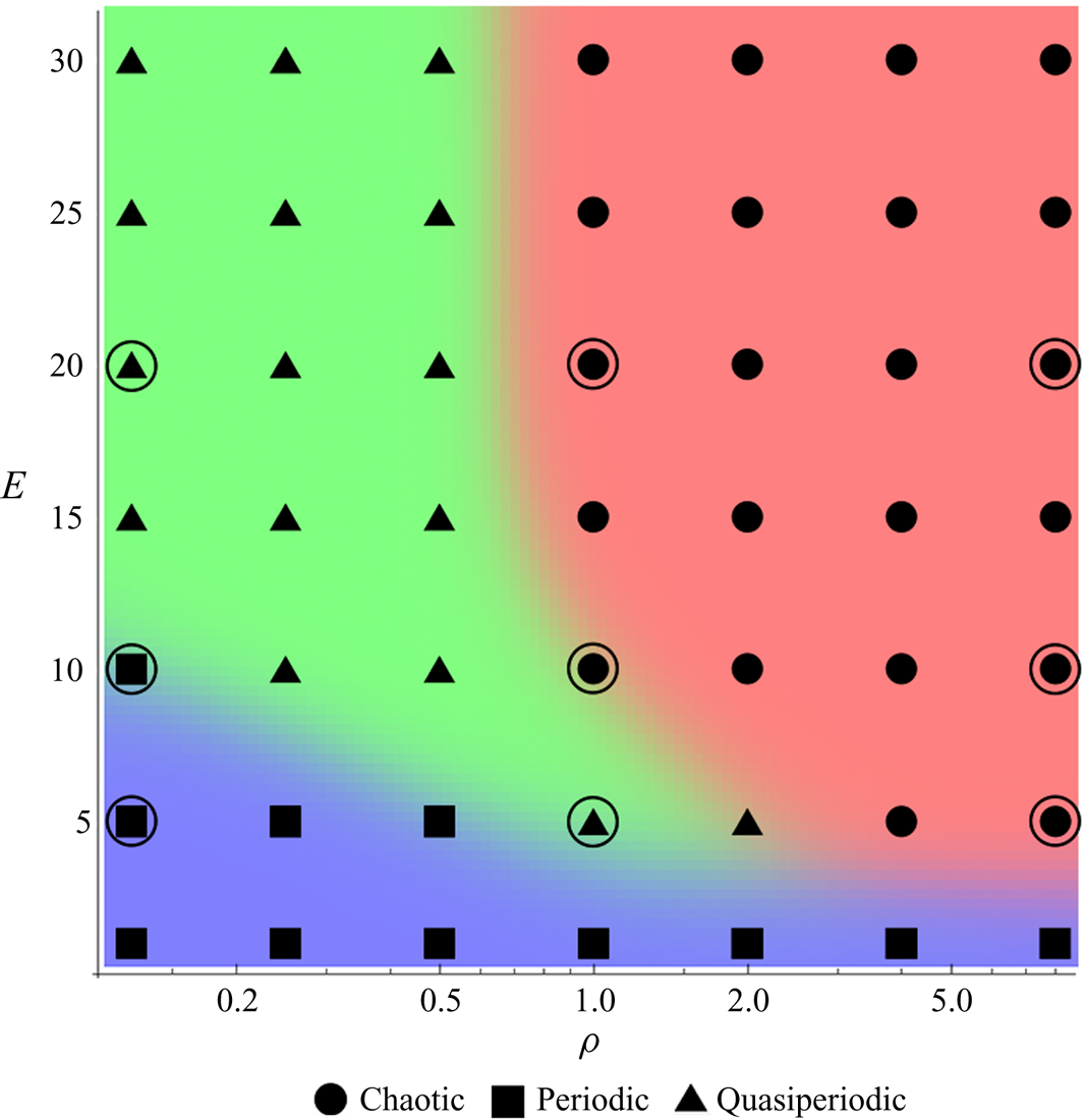
We next zoom in on a smaller portion of the  $\rho -E$ plane, namely
 $(E,\rho )=[(1, \ldots , 30) \times (0.125, \ldots , 8)]$, and fix an initial condition where the ellipsoid was initially set to rotate about the
 $z$-axis, and translate along the
 ${+}y$ direction, these were chosen to ensure that
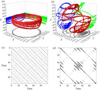
 ${\boldsymbol {L}} \boldsymbol {\cdot } {\boldsymbol {P}} = 0$. At each point in this parameter space, for sufficiently large time series (around 100 000 time steps) an RP was generated. An RQA analysis was then performed and the criteria presented in § 4.4 were used to determine the system behaviour. The progression in the regime space from periodic to quasiperiodic to chaotic is clearly evident in figure 14. Note that while the trend in this regime window is in broad agreement with the boundaries shown in figure 13, specific points may differ because the present figure is the result of one initial condition. Since the computational requirements of GISS are considerable, we selectively performed DNS for the parameter pairs denoted by large circles in this figure. All cases have been run for 100 000 time steps. In each case we obtained the same result from GISS as from the Kirchhoff–Clebsch equations. An example of the DNS results is shown in figure 15, in the form of the orbit tracked by a triaxial ellipsoid along with the resulting RP at two different
 $E$. When
 $E=1$, figure 15(a) shows quasiperiodic behaviour, which is confirmed by the RP in figure 15(c), which shows only regular diagonal lines. Our RQA statistics confirm these conclusions. At the higher energy ratio, here when
 $E = 10$, it can be seen in figure 15(b) that the orbit of the marker point becomes irregular and figure 15(d) reveals its chaotic nature.
Orbital behaviour map of an ellipsoid with aspect ratio  $a\,{:}\,b\,{:}\,c=1\,{:}\,0.8\,{:}\,0.6$ submerged in an inviscid environment for energy ratios
 $1 \le E \le 30$ and density ratios
 $0.125 \le \rho \le 8$ for a single initial condition. A support-vector machine-learning algorithm was used to classify the regions of orbital behaviour. All cases (filled markers) have been characterised using the Kirchhoff–Clebsch equations. Encircled points are those cases cross-validated via inviscid DNS using our GISS solver.

The DNS results: (a,b) Orbits tracked, and (c,d) corresponding RPs by an ellipsoid with aspect ratio  $a\,{:}\,b\,{:}\,c=1\,{:}\,0.8\,{:}\,0.6$ in an inviscid fluid at energy ratios of
 $E = 1, 10$, respectively, and
 $\rho = 1$.
 $(a)$
 $E=1$;
 $(b)$
 $E=10$;
 $(c)$
 $E=1$;
 $(d)$
 $E=10$.

5.1. Departures from sphericity
We may create a triaxial ellipsoid, beginning with a neutrally buoyant sphere of radius  $R$, and stretching outwards by a length
 $\epsilon$ along one axis and inwards along another whilst conserving volume. One would thus obtain a triaxial ellipsoid with the following semiaxes:
 \begin{equation} \left[R(1 + \epsilon), \ R, \ R\left(1 - \frac{\epsilon}{1 + \epsilon} \right) \right]. \end{equation}
It is obvious that we obtain a sphere at  $\epsilon =0$, so
 $\epsilon$ may be called the departure from sphericity parameter. We have seen that any departure from
 $\epsilon =0$ makes the system non-integrable. We vary
 $\epsilon$ in the range
 $10^{-5}$ to
 $1$ going from a near-sphere to a highly triaxial ellipsoid. We choose
 $E=20$. Note that this part of the study uses only one initial condition using the Kirchhoff–Clebsch equations (inviscid). The idea is to show the qualitative dependence of the dynamics on
 $\epsilon$.
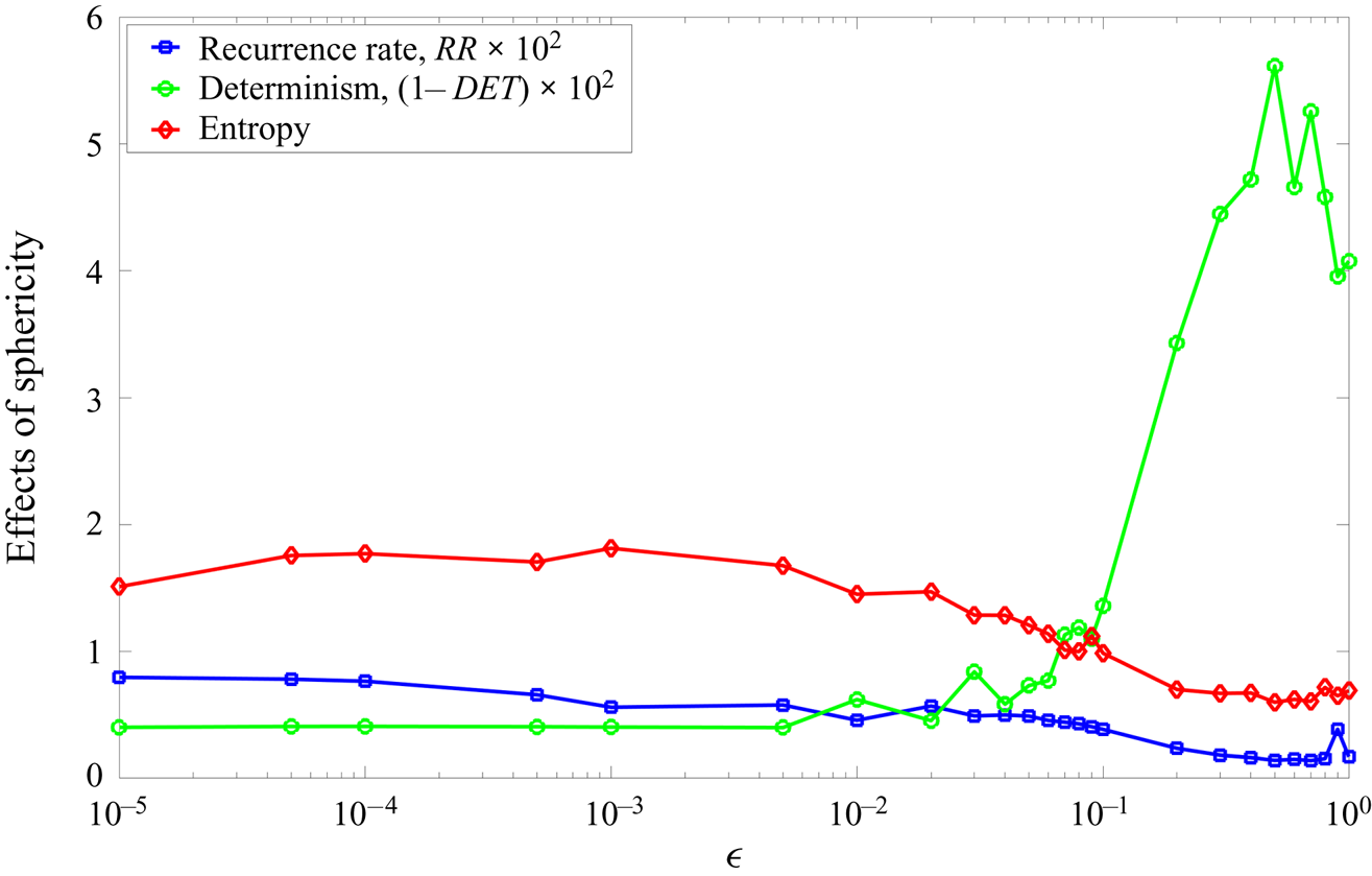
Figure 16 shows the dependence of recurrence rate, determinism and entropy on  $\epsilon$. These RQA statistics were calculated using the entire time series of the respective simulations and they were all of the same length of time (100 000 time-steps). In the range
 $10^{-5} \le \epsilon \le 4 \times 10^{-3}$, when the body is nearly spherical, it exhibits non-chaotic behaviour, as evidenced by
 $(1-DET)\times 10^2$ remaining close to zero. Low non-zero values of
 $\epsilon$ result in periodic behaviour. In the range
 $10^{-2} \le \epsilon \le 10^{-1}$,
 $DET$ demonstrates a small drop; around
 $\epsilon > 10^{-1}$, an abrupt change in the system behaviour is observed. All the RQA parameters switch from non-chaotic to fully chaotic, as
 $DET$ reduces to levels similar to other chaotic systems (presented in the sections above). As per Kozlov & Onishchenko (Reference Kozlov and Onishchenko1982), any of these triaxial ellipsoids satisfies the necessary conditions for non-integrability. However, our results show that there is a critical departure from sphericity below which it is easier to obtain periodic orbits. The nearly spherical cases have a relatively high recurrence rate and high entropy, which indicates small Lyapunov exponents (Cencini, Cecconi & Vulpiani Reference Cencini, Cecconi and Vulpiani2010). It could be argued that the abrupt change in behaviour at
 $\epsilon =10^{-1}$ corresponds to Lyapunov timescales becoming shorter.
The dependency of the recurrence rate, determinism and entropy on  $\epsilon$, which is the perturbation from the aspherical shape obtained by solving the Kirchhoff–Clebsch equations. The volume of the ellipsoid is kept constant as
 $\epsilon$ is varied, at
 $E = 20$ and
 $\rho = 1$.

6. Orbits in viscous environments
Our study so far has been on an inviscid fluid and it is natural to ask what would happen in a real fluid. Viscous drag could have a dampening effect, but more important, it could be asked if vortex shedding would introduce chaos into the system, even rendering the inviscid study irrelevant. We show in this section that in a viscous case as well, added mass continues to be an important player, and insights obtained from the above study are important in understanding the behaviour. In fact it has been recently shown that is possible to extend the notion of added mass from the ideal fluid regime to more general viscous flows (Limacher, Morton & Wood Reference Limacher, Morton and Wood2018). We also point out how vortex shedding indeed can change the dynamics, and in particular give rise to chaotic orbits executed by a spheroid. Thus while the earlier sections elucidated the role of added mass, its combination with viscous forces is presented here to complete the study.
We define the ellipsoid Reynolds number as  $Re_p = a U_0 /\nu$, where
 $a$ is length of the major axis,
 $U_0$ is a characteristic velocity here chosen as the magnitude of the initial translational velocity
 ${\boldsymbol {v}}$ given to the ellipsoid, and
 $\nu$ is the kinematic viscosity of the surrounding fluid. Considering that the velocity of the solid evolves during the simulation, this
 $Re_p$ must be treated as an indicative value. The motion of the solid is essentially dependent on the accurate resolution of flow (and hence, viscous drag) immediately around the body and the exact imposition of the no-slip boundary condition.
6.1. Motion of a triaxial ellipsoid in viscous fluid
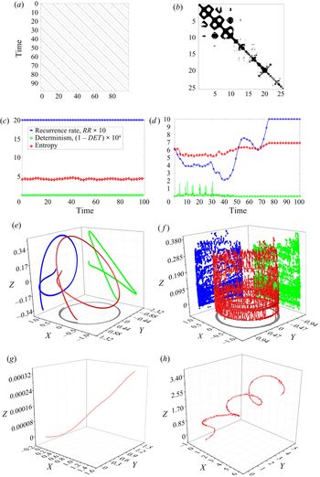
Figure 17 shows the dynamics of a triaxial ellipsoid with  $Re_p=10\,000$. As in the inviscid case, the motion is non-chaotic at small
 $E$ and chaotic at larger
 $E$. This shows that despite viscosity affording vortex shedding, the inviscid predictions (for the same initial conditions) are a good indicator of the initial behaviour of an ellipsoid in a real fluid in this case. However, the chaotic nature is suppressed as time progresses, presumably because of viscous damping. First, the angular velocities become vanishingly small while the ellipsoid continues to translate. Eventually, we expect the ellipsoid to come to a halt.
Motion of a triaxial ellipsoid with aspect ratio  $a\,{:}\,b\,{:}\,c=1\,{:}\,0.8\,{:}\,0.6$ in viscous fluid,
 $Re_p=10\,000$,
 $\rho = 1$. The behaviour is similar to the inviscid case.
 $(a)$
 $E=1$, recurrence;
 $(b)$
 $E=20$, recurrence;
 $(c)$
 $E=1$, RQA statistics;
 $(d)$
 $E=20$, RQA statistics;
 $(e)$
 $E=1$, marker orbit;
 $(\,f)$
 $E=20$, marker orbit;
 $(g)$
 $E=1$, centroid trajectory;
 $(h)$
 $E=20$, centroid trajectory.

6.2. Motion of a prolate spheroid in viscous fluid
We have seen that prolate spheroids can display no chaos in inviscid environments. Here, we consider the same ellipsoid of revolution  $(a\,{:}\,b\,{:}\,c=1\,{:}\,0.7\,{:}\,0.7)$ subjected to an impulse in a viscous environment characterised by
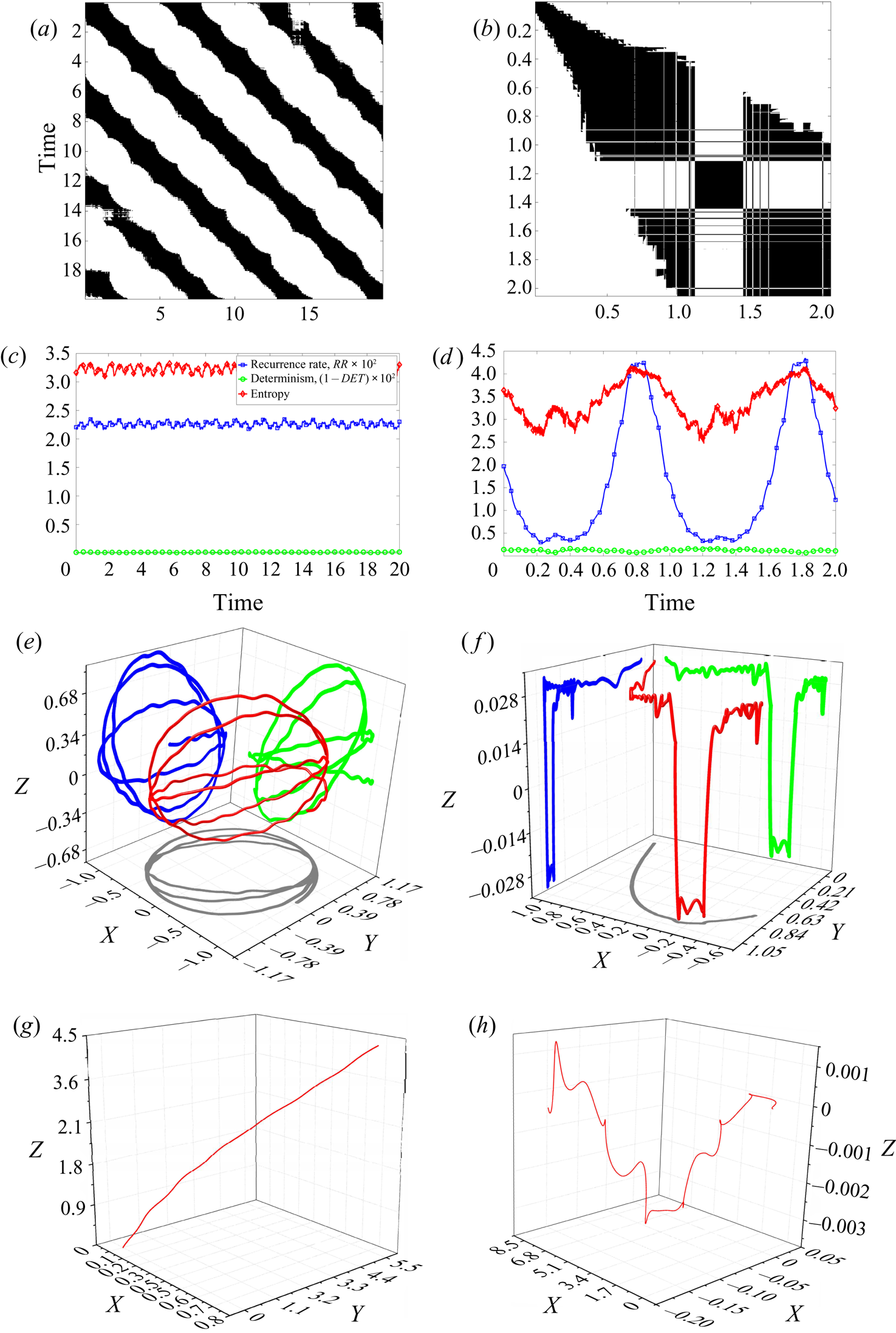
 $Re_p = 10\,000$. Our DNS results presented in figure 18 demonstrate a complex pattern of orbital behaviour. At
 $E=1$, the orbit is demonstrably non-chaotic. It must be recalled from figures 6(a), 9(a) and 10(a) that in an inviscid environment under identical initial conditions, the prolate spheroid tracks a quasiperiodic orbit. This case also presents an opportunity for rigorous testing of the numerical convergence of GISS, and for evaluating its performance and higher Reynolds numbers. We considered an ellipsoid of revolution with dimensions
 $a\,{:}\,b\,{:}\,c=1\,{:}\,0.7\,{:}\,0.7$ at an
 $Re_p=10\,000$ and energy ratio,
 $E=1$. At very long times, due to frictional losses, the system would come to a stop, but at this high
 $Re_p$, for a large number of time periods, the motion lies very close to a non-chaotic orbit. Our simulations at mesh refinement levels of
 $R_m=2^{11}, 2^{12}, 2^{13}$ demonstrated that the orbits tracked were indeed practically closed, indicating periodicity. It must be noted that these mesh resolutions correspond to 9M, 10M and 11.3M elements, respectively, with around 200 000 Lagrangian elements on the ellipsoid. It must be noted that 11.3M elements was the maximum possible resolution at which we could run our simulations. In addition, the spatial dynamics of the orbits tracked also matched well with each other, indicating numerical convergence. In particular the trajectories from
 $R_m=2^{12}$ and
 $R_m= 2^{13}$ were practically indistinguishable. We checked that with
 $R_m=2^{12}$ the smallest grid within the boundary layer close to the body was at least
 $16$ times smaller than the boundary layer thickness, and was often finer. Note that the boundary layer at this Reynolds number is unlikely to be turbulent, except maybe in a small portion at the rear of the body. The GISS follows a rigorous vorticity-based criterion to increase grid refinement, and these arguments lend support to our expectation that the resolution is sufficient. This flow is unsteady and we need differently refined grids as time progresses in the boundary layer and in the wake. The dynamic adaptive gridding is thus ideally suited for this computation.
Motion of a prolate spheroid with aspect ratio  $a\,{:}\,b\,{:}\,c=1\,{:}\,0.7\,{:}\,0.7$ in viscous fluid,
 $Re_p=10\,000$,
 $\rho = 1$. The dynamics at high
 $E$, unlike in the inviscid case, is chaotic, but different from that seen in inviscid chaotic dynamics of a triaxial ellipsoid.
 $(a)$
 $E=1$, recurrence;
 $(b)$
 $E=20$, recurrence;
 $(c)$
 $E=1$, RQA statistics;
 $(d)$
 $E=20$, RQA statistics;
 $(e)$
 $E=1$, marker orbit;
 $(\,f)$
 $E=20$, marker orbit;
 $(g)$
 $E=1$, centroid trajectory;
 $(h)$
 $E=20$, centroid motion.

At  $E=20$, the prolate spheroid in viscous fluid tracks a chaotic orbit that does not dampen completely within the simulation time. This is unlike a prolate spheroid under any conditions in inviscid fluid. An examination of the trajectories of the marker point in figure 18(f), and the centroid in figure 18, however, reveal an important feature: that the trajectory is practically planar, with the centroid effectively confined to the
 $x\text {--}z$ plane and the marker point nearly so. This is an example of the restricted dynamics that a prolate spheroid can execute, given that the extra symmetries in the added mass tensor were shown to produce an additional integral
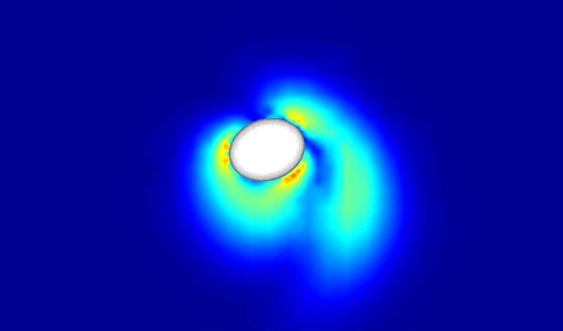
 $l_1$ in inviscid flow. This integral effectively restricts interesting angular momentum exchanges to the plane perpendicular to the unequal axis. We thus see that added mass effects are strong in viscous flow as well. To isolate the cause of chaos, we plot a picture of the instantaneous vorticity field around the prolate spheroid obtained from our DNS in figure 19. A partially detached vortex can be seen. This vortex distorts the surface pressure field, giving rise to asymmetric force and torque. As successive vortices are generated and shed, the ellipsoid will be disturbed from a periodic orbit. Thus viscosity breaks the symmetry of the system by irregular vortex shedding.
The vorticity field around a neutrally buoyant ellipsoid with aspect ratio  $a\,{:}\,b\,{:}\,c=1\,{:}\,0.7\,{:}\,0.7$ at
 $Re_p=10\,000$ and
 $E = 20$. The colour shading is proportional to
 $| \boldsymbol {\nabla } \times {\boldsymbol {u}} |$. Irregular vortex shedding can be seen.

In our viscous simulations therefore, we see the effects of added mass: in keeping the dynamics periodic for smaller energy ratios, while restricting variations in the rotational dynamics to two dimensions (in the body-fixed frame). We also see the effects of viscosity, in producing chaos where there was none by vortex shedding, and by suppressing chaos at long time by dissipation. We have also conducted simulations at lower Reynolds numbers (not shown) in which viscous damping dominates.
7. Conclusion
To summarise, we have studied conditions under which chaotic motion is displayed by an ellipsoid in inviscid and viscous flow. We identify five non-dimensional numbers which affect the dynamics: the ratios  $b/a$ and
 $c/a$ of the ellipsoid axes, the fluid/solid density ratio
 $\rho$, the ratio
 $E$ of initial kinetic energy in translational to rotational motion, and the particle Reynolds number. In the inviscid case, we were aided by the Kozlov–Onishchenko theorem. We have identified a new integral of the motion for the dynamics of a spheroid: the component of generalised angular momentum along the unequal axis. Though it is implicit in the Kozlov–Onishchenko theorem that there must exist such an integral, its identification explains the physics for both inviscid and viscous flow.
We solve the Kirchhoff–Clebsch equations over a very large parameter range of  $\rho$ and
 $E$ and show that the propensity for chaos (fraction of disintegrated tori in phase space) in a triaxial ellipsoid depends strongly on these quantities. To distinguish chaotic behaviour from periodic and quasiperiodic we use RQA, Poincare sections and orbit maps. In the limit of zero density ratio we confirm that the system supports an additional integral of motion, by which the dynamics reduces to the classical problem of an ellipsoid in vacuum. Thus we clarify how added mass is the cause of chaos. We show how the added mass tensor for a general ellipsoid provides a vehicle for exchange of energy between fluid and solid and between rotation and translation. The motion is also shown to be periodic in the limit of zero initial translation. We show that high fluid densities and intermediate values of the initial kinetic energy ratio increase chaos in the system. We thus identify ranges in parameter space where the system is non-integrable but chaos is rarely attainable.
We have developed a solid–fluid solver, GISS, using the immersed boundary methodology and the open source DNS fluid solver, Gerris. The solver can simulate the 6DOF motion of solid bodies in both inviscid and viscous fluid and calculate the hydrodynamic force applied on the solid accurately. Our numerical method passes stringent validations including displaying the same behaviour in the  $\rho -E$ plane as the Kirchhoff–Clebsch equations. Given that problems of bodies freely moving in fluids have been simulated far less than the flow past fixed bodies, we hope that this solver will enable future research in this direction.
With GISS, we are able to demonstrate how added mass and viscosity affect the dynamics of an ellipsoid. For a triaxial ellipsoid, the added mass dominates the behaviour, with the high Reynolds number and inviscid cases behaving similarly at early times. At later times, viscous damping simplifies chaotic dynamics to periodic before halting it completely. We show that asymmetric vortex shedding can cause chaotic dynamics in a spheroid, where the Kozlov–Onishchenko theorem bans chaos in inviscid flow. However, the extra integral we identified in inviscid flow influences the viscous flow as well, causing spheroidal orbits to be more limited in phase space than those of a triaxial ellipsoid.
We can envisage that our study will be of relevance to practical applications such as designing efficient magnetic stirrers of ellipsoidal shapes, and in studying the dynamics of non-spherical particles. Auguste et al. (Reference Auguste, Magnaudet and Fabre2013) showed how the dynamics of a body which is free to move is far richer than that of one which is held fixed with flow going past it. Our work has brought out many new features and possibilities for a far richer dynamics due to the departure from a spheroidal shape of the body. Whether in viscous or in inviscid flow, this is shown to be directly related to the increased complexity of the added mass tensor. We hope this will encourage more studies on the many unexplored aspects of these and even more general shaped bodies moving in a fluid.
Acknowledgements
The authors acknowledge the EC-RISE-ThermaSMART project. This project has received funding from the European Union's Horizon 2020 research and innovation programme under the Marie Skłodowska-Curie grant agreement no. 778104. R.G. acknowledges support of the Department of Atomic Energy, Government of India, under project no. 12-R&D-TFR-5.10-1100 and thanks A. Leonard for bringing this class of problems to her attention many years ago.
Declaration of interests
The authors report no conflict of interest.