1 Introduction
Flows over curved surfaces occur in a wide range of applications including airfoils, compressor and turbine vanes as well as aerial, naval and ground vehicles. In most of these applications the surface has convex curvature, while concave surfaces are less common. Boundary layers over concave surfaces are prone to the Görtler instability, a linear instability mechanism arising from centrifugal forces (Görtler Reference Görtler1941). The Görtler instability corresponds to counter-rotating streamwise vortices with constant spanwise wavelength that become linearly unstable and grow toward breakdown to turbulence. Hall (Reference Hall1990), Floryan (Reference Floryan1991) and Saric (Reference Saric1994) provide thorough reviews of theoretical, numerical and experimental studies of the Görtler instability. Floryan (Reference Floryan1986) developed stability criteria for the Görtler instability over concave and convex walls. For the concave case, the Blasius and wall jet profiles (inner part of the wall jet) are potentially unstable, whereas for the convex case only the wall jet is potentially unstable (outer part of the wall jet). Monotonic boundary-layer flows over convex walls are exponentially stable. Consequently, they have received considerably less attention than flows over concave walls. The majority of studies investigating the primary Görtler instability, its secondary instabilities and transition to turbulence have concentrated on flows over concave surfaces (e.g. Floryan & Saric Reference Floryan and Saric1982; Swearingen & Blackwelder Reference Swearingen and Blackwelder1987; Liu & Domaradzki Reference Liu and Domaradzki1993; Goulpié, Klingmann & Bottaro Reference Goulpié, Klingmann and Bottaro1996; Rogenski, de Souza & Floryan Reference Rogenski, de Souza and Floryan2016) or wall jet flows over convex surfaces (e.g. Matsson Reference Matsson1995; Le Cunff & Zebib Reference Le Cunff and Zebib1996; Matsson Reference Matsson2008).
Nevertheless, several studies have addressed the evolution of Görtler vortices on convex surfaces. Kalburgi, Mangalam & Dagenhart (Reference Kalburgi, Mangalam and Dagenhart1988) investigated the Görtler instability in the flow over an airfoil with a concave region, followed by a convex region. They found that as the flow enters the convex region, the initial counter-rotating vortices lift off the surface and dissipate, while another layer of vortices with opposite sign of rotation develops near the surface. Consequently, in the convex region the streamwise velocity perturbations shift by half a wavelength in the spanwise direction. In addition, Mangalam et al. (Reference Mangalam, Dagenhart, Hepner and Meyers1985) and Mangalam, Dagenhart & Kalburgi (Reference Mangalam, Dagenhart and Kalburgi1987) reported the occasional merging of the vortices in the convex region. Similar findings have been reported by Benmalek & Saric (Reference Benmalek and Saric1994), who investigated the evolution of Görtler vortices, created in a concave section, over a periodically curved wall. They observed that the Görtler vortices are strengthened in the concave regions while the convex regions stabilize the Görtler vortices. Another configuration examined by Benmalek & Saric (Reference Benmalek and Saric1994) corresponds to a concave section, followed by a long convex section. They found that in the convex section new sets of vortices are successively created with opposite rotation to the preceding set.
In all of the above studies the spatial initial conditions for the flow over the convex surface correspond to Görtler vortices together with the streaks created by the vortices. It is hard to isolate the effect of the streaks on the overall evolution of the flow over the convex surface, i.e. to identify the connection between the streak shape and the damping of the vortices. Moreover, in possible flow control applications, involving counter-rotating vortices created by vortex generators or jets installed near a wing’s leading edge, only a pair of vortices (without streaks) is formed. Therefore, it is useful to investigate the effect of spatial initial conditions for the flow over a convex surface. The effect of vortex generators on the flow in various geometrical configurations is investigated by Pearcey (Reference Pearcey and Lachmann1961) in the context of separation delay. A detailed account of the mechanism leading to the creation of a pair of counter-rotating streamwise vortices due to the interaction between a jet and cross-flow can be found in the review by Mahesh (Reference Mahesh2013).
The absence of exponential instabilities in the flow over a convex wall does not necessarily imply that disturbances may not grow and lead to turbulence. Non-modal transient growth can allow disturbances to grow even in a linearly stable flow and significantly change the base state (see Schmid Reference Schmid2007), so that the modified flow becomes unstable to secondary infinitesimal disturbances (e.g. Karp & Cohen Reference Karp and Cohen2017). It is known that the optimal linear transient growth corresponds to streamwise vortices in plane Couette and Poiseuille flows (Butler & Farrell Reference Butler and Farrell1992). Investigations of transient growth in flat plate boundary layers, which are non-parallel, yielded a similar vortical structure corresponding to counter-rotating streamwise vortices (Andersson, Berggren & Henningson Reference Andersson, Berggren and Henningson1999; Luchini Reference Luchini2000). Transient growth studies of flows over convex surfaces will provide the optimal disturbance inflow conditions. An open question is whether the optimal structure for transient growth over convex surfaces is similar to that of Görtler instability over concave surfaces.
The general relevance of transient growth analysis to boundary layers exposed to free-stream turbulence has been established by comparing the theoretical predictions to simulations and experiments. The simulations of Jacobs & Durbin (Reference Jacobs and Durbin2001), validated against the experiment by Roach & Brierley (Reference Roach and Brierley1990), revealed that the dominant spanwise wavelength of the streaks,
 $\unicode[STIX]{x1D6FD}\approx 1.4\unicode[STIX]{x1D6FF}$
, is consistent with the optimal growth analyses of Butler & Farrell (Reference Butler and Farrell1992), Andersson et al. (Reference Andersson, Berggren and Henningson1999) and others. Similar values were also reported in the measurements by Westin et al. (Reference Westin, Boiko, Klingmann, Kozlov and Alfredsson1994). Additional comparisons between experiments and theory were reported for instance by Matsubara & Alfredsson (Reference Matsubara and Alfredsson2001). They confirmed the growth of the perturbations to be proportional to
 $x^{1/2}$
as predicted by the linear theory. Moreover, they showed that the normal fluctuation profiles agree with those found in the transient growth analyses by Andersson et al. (Reference Andersson, Berggren and Henningson1999) and Luchini (Reference Luchini2000). Conditional sampling of streaks in boundary layers exposed to free-stream turbulence has been performed by Hack & Zaki (Reference Hack and Zaki2015). They determined that the conditional average of the streaks matches the optimal growth analysis. Therefore, the analysis of linear transient growth can be interpreted as a type of a reduced-order model for investigations of the underlying flow physics of disturbance growth.
The secondary instabilities of streaks, formed during the growth of Görtler vortices over a concave surface, were investigated by Swearingen & Blackwelder (Reference Swearingen and Blackwelder1987). Although a concave surface was considered, the motivation for the study was to model the eddy structures found in transitional and turbulent flat plate boundary layers. They emphasized the role of the spanwise inflection points in the transition mechanism. Andersson et al. (Reference Andersson, Brandt, Bottaro and Henningson2001) investigated the secondary instabilities of streaks in a flat plate boundary layer. An inviscid analysis of nonlinearly modified streaks, obtained by direct numerical simulations (DNS), was conducted. It was found that the most dangerous disturbances are sinuous subharmonic (with respect to the high-speed streak), with a critical streak amplitude of 26 %. Fundamental sinuous modes follow closely with a critical amplitude of 28 % and the varicose modes have appreciably higher critical amplitudes of 37 %. Vaughan & Zaki (Reference Vaughan and Zaki2011) extended the analysis to unsteady, low frequency, streaks. The instabilities were classified as inner, fundamental varicose, and outer, subharmonic sinuous, modes, the latter becoming unstable for amplitudes as low as 17 %. Hack & Zaki (Reference Hack and Zaki2014) performed secondary instability analysis of streaks triggered by free-stream turbulence. They showed that Blasius boundary layers prefer outer instabilities, whereas adverse pressure gradient boundary layers favour the inner mode. Hack & Zaki (Reference Hack and Zaki2016) devised a scheme for predicting transition, based on artificial neural networks. The scheme achieved a higher accuracy of identifying unstable streaks at considerably lower computational cost, compared with linear stability theory. In the current study the effects of the curvature on the various types of secondary instabilities are investigated and compared with their counterparts for flat plate boundary layers.
Our aim is to identify the physical mechanism of transient growth in flows over convex surfaces, its secondary instabilities and subsequent transition to turbulence. We analyse the role and significance of various parameters (e.g. geometry, disturbance wavenumbers and frequencies) in the process. The mathematical methods are described in § 2, followed by optimal disturbances found using local stability theory in § 3 and DNS of the optimal disturbances in § 4. Secondary stability analyses of the modified flow are presented in § 5, and DNS of secondary instabilities are discussed in § 6. Preliminary studies of transient growth over a spiral surface are presented in § 7. The paper ends with concluding remarks in § 8.
2 Mathematical methods
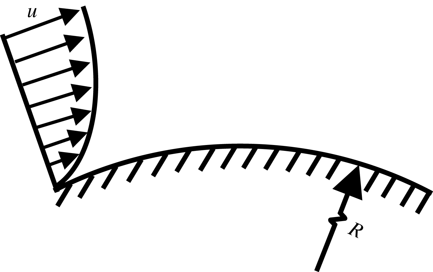
We consider the flow over a convex surface with radius
 $R$
, as shown in figure 1. The velocity field is denoted by
 $\boldsymbol{u}(t,x,y,z)=(u,v,w)^{\text{T}}$
, where
 $u,v$
and
 $w$
are the velocity components in the streamwise (curvilinear along the wall), wall-normal and spanwise coordinates (
 $x,y,z$
), respectively, and
 $t$
is time. Length scales are normalized by the boundary-layer thickness,
 $\unicode[STIX]{x1D6FF}$
, velocities are normalized by the free-stream velocity,
 $U_{\infty }$
, and time by
 $\unicode[STIX]{x1D6FF}/U_{\infty }$
.
Boundary layer over a convex surface.

Similar to concave surfaces, we define the Görtler number
 $$\begin{eqnarray}\widetilde{G\ddot{o} }=\frac{U_{\infty }\unicode[STIX]{x1D6FF}}{\unicode[STIX]{x1D708}}\left(\frac{\unicode[STIX]{x1D6FF}}{R}\right)^{1/2},\end{eqnarray}$$
where
 $\unicode[STIX]{x1D708}$
is the kinematic viscosity. Note that
 $\widetilde{G\ddot{o} }$
is defined here as a non-dimensional curvature parameter and does not imply the presence of Görtler instability. Defining the Reynolds number
 $Re=U_{\infty }\unicode[STIX]{x1D6FF}/\unicode[STIX]{x1D708}$
and the normalized curvature by
 $\unicode[STIX]{x1D705}=\unicode[STIX]{x1D6FF}/R$
, the Görtler number is given by
 $$\begin{eqnarray}\widetilde{G\ddot{o} }=Re\sqrt{\unicode[STIX]{x1D705}}.\end{eqnarray}$$
The transient growth calculations are based on a local stability approach. Non-parallel and nonlinear effects are captured by prescribing the optimal solution as an inflow condition to DNS. Details are given below.
2.1 Local stability analysis
For flows over concave surfaces it has been found that local stability analysis is valid only in the small spanwise wavelength limit and, the correct approach involves a downstream-marching solution (parabolic stability equations) as first proposed by Hall (Reference Hall1983). Nevertheless, the results depend on the initial condition, which may grow transiently before evolving into a Görtler mode (Lee & Liu Reference Lee and Liu1992). Several studies have compared local and marching solutions (e.g. Goulpié et al. Reference Goulpié, Klingmann and Bottaro1996; Le Cunff & Zebib Reference Le Cunff and Zebib1996). Bottaro & Luchini (Reference Bottaro and Luchini1999) found that above a certain Görtler number both local and marching solutions yield similar results.
In the current study, local stability analysis is utilized to identify the general trends and effects of parameters, while the exact evolution is calculated by DNS. Floryan & Saric (Reference Floryan and Saric1982) have shown that in the large-
 $Re$
limit the effect of the curvature on the boundary-layer profile is minor and the latter is well described by the Blasius solution.
Assuming parallel flow, the velocity field is given by
 $$\begin{eqnarray}\boldsymbol{u}_{t}=(U_{B}(y),0,0)^{\text{T}}+\unicode[STIX]{x1D700}\boldsymbol{u},\end{eqnarray}$$
where
 $U_{B}(y)$
is given by the Blasius solution. Retaining only the leading-order terms as a result of curvature leads to the following disturbance equations, first obtained by Görtler (Reference Görtler1941):
 $$\begin{eqnarray}\displaystyle & \displaystyle \frac{\unicode[STIX]{x2202}u}{\unicode[STIX]{x2202}t}+U_{B}\frac{\unicode[STIX]{x2202}u}{\unicode[STIX]{x2202}x}+U_{B}^{\prime }v+\frac{\unicode[STIX]{x2202}p}{\unicode[STIX]{x2202}x}=\frac{1}{Re}\unicode[STIX]{x1D6FB}^{2}u, & \displaystyle\end{eqnarray}$$
 $$\begin{eqnarray}\displaystyle & \displaystyle \frac{\unicode[STIX]{x2202}v}{\unicode[STIX]{x2202}t}-2\unicode[STIX]{x1D705}U_{B}u+U_{B}\frac{\unicode[STIX]{x2202}v}{\unicode[STIX]{x2202}x}+\frac{\unicode[STIX]{x2202}p}{\unicode[STIX]{x2202}y}=\frac{1}{Re}\unicode[STIX]{x1D6FB}^{2}v, & \displaystyle\end{eqnarray}$$
 $$\begin{eqnarray}\displaystyle & \displaystyle \frac{\unicode[STIX]{x2202}w}{\unicode[STIX]{x2202}t}+U_{B}\frac{\unicode[STIX]{x2202}w}{\unicode[STIX]{x2202}x}+\frac{\unicode[STIX]{x2202}p}{\unicode[STIX]{x2202}z}=\frac{1}{Re}\unicode[STIX]{x1D6FB}^{2}w, & \displaystyle\end{eqnarray}$$
 $$\begin{eqnarray}\displaystyle & \displaystyle \frac{\unicode[STIX]{x2202}u}{\unicode[STIX]{x2202}x}+\frac{\unicode[STIX]{x2202}v}{\unicode[STIX]{x2202}y}+\frac{\unicode[STIX]{x2202}w}{\unicode[STIX]{x2202}z}=0. & \displaystyle\end{eqnarray}$$
 $$\begin{eqnarray}\boldsymbol{q}=\hat{\boldsymbol{q}}(y)\text{e}^{\text{i}(\unicode[STIX]{x1D6FC}x+\unicode[STIX]{x1D6FD}z-\unicode[STIX]{x1D714}t)},\end{eqnarray}$$
where
 $\boldsymbol{q}=(u,v,w,p)^{\text{T}}$
,
 $\unicode[STIX]{x1D714}$
is the frequency,
 $\unicode[STIX]{x1D6FD}$
is the spanwise wavenumber and
 $\unicode[STIX]{x1D6FC}$
is the spatial complex eigenvalue. The eigenvalue problem is solved using a spectral method and a mapping of the Chebyshev interval
 ${\hat{y}}\in [-1,1]$
to the physical domain
 $y\in [0,y_{max}]$
, such that (Hanifi, Schmid & Henningson Reference Hanifi, Schmid and Henningson1996)
 $$\begin{eqnarray}y=a\frac{1+{\hat{y}}}{b-{\hat{y}}},\quad a=\frac{y_{i}y_{max}}{y_{max}-2y_{i}},\quad b=1+\frac{2a}{y_{max}},\end{eqnarray}$$
which maps half of the grid points to the interval
 $y\in [0,y_{i}]$
. In the current study 200 Chebyshev polynomials are used with
 $y_{max}=7$
and
 $y_{i}=1.4$
.
2.2 Transient growth
Transient growth is a mechanism which allows disturbances to amplify in linearly stable flows. The growth is bounded and ultimately overcome by viscous decay; however, during the transient growth the base flow may be modified significantly and become unstable to infinitesimal secondary disturbances. In the current study we consider the spatial amplification of disturbances in a parallel flow. The linear transient growth is calculated from the gain,
 $G(x)=E(x)/E_{0}$
, of the disturbance kinetic energy,
 $E(x)=(\boldsymbol{q}(x),\boldsymbol{q}(x))_{E}$
, at location
 $x$
normalized by its value at the inflow,
 $E_{0}=E(x=0)$
, with the energy norm given by
 $$\begin{eqnarray}(\boldsymbol{q}_{i},\boldsymbol{q}_{j})_{E}=\frac{1}{2TL_{z}}\int _{0}^{L_{z}}\int _{0}^{\infty }\int _{0}^{T}(u_{i}^{\ast }u_{j}+v_{i}^{\ast }v_{j}+w_{i}^{\ast }w_{j})\,\text{d}t\,\text{d}y\,\text{d}z,\end{eqnarray}$$
where
 $T=2\unicode[STIX]{x03C0}/\unicode[STIX]{x1D714}$
and
 $L_{z}=2\unicode[STIX]{x03C0}/\unicode[STIX]{x1D6FD}$
.
The procedure is briefly described below, and the reader is referred to Schmid & Henningson (Reference Schmid and Henningson2001) for the details. For given parameters
 $Re$
,
 $\unicode[STIX]{x1D714}$
,
 $\unicode[STIX]{x1D6FD}$
and
 $\unicode[STIX]{x1D705}$
, first the eigenvalue problem is solved to obtain the eigenvalues
 $\unicode[STIX]{x1D6FC}$
and the eigenfunctions
 $\hat{\boldsymbol{q}}(y)$
. The velocity is written as
 $$\begin{eqnarray}\boldsymbol{q}=\tilde{\boldsymbol{q}}(x,y)\text{e}^{\text{i}(\unicode[STIX]{x1D6FD}z-\unicode[STIX]{x1D714}t)},\end{eqnarray}$$
with
 $$\begin{eqnarray}\tilde{\boldsymbol{q}}(x,y)\triangleq \mathop{\sum }_{n=1}^{\infty }c_{n}\hat{\boldsymbol{q}}_{n}(y)\text{e}^{\text{i}\unicode[STIX]{x1D6FC}_{n}x},\end{eqnarray}$$
where
 $\boldsymbol{c}$
are expansion coefficients of the eigenmodes and
 $\tilde{\boldsymbol{q}}(x,y)$
is introduced for convenience. Next, the energy norm matrix is calculated:
 $$\begin{eqnarray}\unicode[STIX]{x1D614}_{i,j}=(\boldsymbol{q}_{i},\boldsymbol{q}_{j})_{E}.\end{eqnarray}$$
This matrix is Hermitian positive-definite and can be decomposed via Cholesky factorization,
 $\unicode[STIX]{x1D648}=\unicode[STIX]{x1D641}^{H}\unicode[STIX]{x1D641}$
, where the superscript
 $H$
implies the Hermitian (conjugate) transpose. This allows connection of the energy norm to the
 $L_{2}$
norm via the relation
 $$\begin{eqnarray}(\boldsymbol{q}_{i},\boldsymbol{q}_{j})_{E}=c_{i}^{H}\unicode[STIX]{x1D648}c_{j}=c_{i}^{H}\unicode[STIX]{x1D641}^{H}\unicode[STIX]{x1D641}c_{j}=(\unicode[STIX]{x1D641}c_{i},\unicode[STIX]{x1D641}c_{j})_{2}.\end{eqnarray}$$
The maximal possible amplification is given by
 $$\begin{eqnarray}G(x)=\max _{\boldsymbol{q}_{0}}\frac{\Vert \boldsymbol{q}(x)\Vert _{E}^{2}}{\Vert \boldsymbol{q}_{0}\Vert _{E}^{2}}=\max _{\boldsymbol{c}_{0}}\frac{\Vert \unicode[STIX]{x1D641}\boldsymbol{c}(x)\Vert _{2}^{2}}{\Vert \unicode[STIX]{x1D641}\boldsymbol{c}_{0}\Vert _{2}^{2}}=\Vert \unicode[STIX]{x1D641}\text{e}^{\text{i}\unicode[STIX]{x1D726}x}\unicode[STIX]{x1D641}^{-1}\Vert _{2}^{2},\end{eqnarray}$$
where
 $\unicode[STIX]{x1D726}=\text{diag}\{\unicode[STIX]{x1D6FC}_{1},\unicode[STIX]{x1D6FC}_{2},\ldots \}$
. It should be noted that this procedure gives the envelope for all possible maximum energy amplifications, in which, for each position,
 $x$
is optimized over all possible inflow conditions. The specific inflow condition achieving a maximum at a certain
 $x$
is given by a singular value decomposition of the matrix exponential. Convergence studies showed that 200 eigenmodes are sufficient to capture the growth for a wide range of parameters.
2.3 Secondary stability analysis
The optimal linear transient growth for wall-bounded flows occurs for an initial condition describing counter-rotating streamwise vortices. The vortices generate streaks which vary slowly with respect to the streamwise coordinate. The analysis assumes a separation of scales, between the base flow and the secondary instability. The underlying hypothesis is that the scale on which the base flow changes is significantly longer than the secondary instability scale such that any changes in the base flow on this scale are negligible and the streamwise coordinate can be used as a parameter. In addition, the cross-stream components are considerably smaller than the streamwise component and therefore can be neglected. The above two simplifications are valid for streaks in boundary layers over convex surfaces, as shown in the results section. Therefore, the secondary instability of the streaks is studied by considering a parallel base flow at a given
 $x$
location. The stability analysis is based on a Floquet expansion in span as the base flow is inhomogeneous in the
 $y{-}z$
plane (e.g. Karp & Cohen Reference Karp and Cohen2014).
The modified base flow,
 $U(y,z;x)$
, consists of a two-dimensional boundary layer and spanwise periodic streaks. Retaining only the leading-order terms as a result of curvature, the linearized secondary stability equations are
 $$\begin{eqnarray}\displaystyle & \displaystyle \frac{\unicode[STIX]{x2202}u_{d}}{\unicode[STIX]{x2202}t}+U\frac{\unicode[STIX]{x2202}u_{d}}{\unicode[STIX]{x2202}x}+\frac{\unicode[STIX]{x2202}U}{\unicode[STIX]{x2202}y}v_{d}+\frac{\unicode[STIX]{x2202}U}{\unicode[STIX]{x2202}z}w_{d}+\frac{\unicode[STIX]{x2202}p_{d}}{\unicode[STIX]{x2202}x}=\frac{1}{Re}\unicode[STIX]{x1D6FB}^{2}u_{d}, & \displaystyle\end{eqnarray}$$
 $$\begin{eqnarray}\displaystyle & \displaystyle \frac{\unicode[STIX]{x2202}v_{d}}{\unicode[STIX]{x2202}t}-2\unicode[STIX]{x1D705}Uu_{d}+U\frac{\unicode[STIX]{x2202}v_{d}}{\unicode[STIX]{x2202}x}+\frac{\unicode[STIX]{x2202}p_{d}}{\unicode[STIX]{x2202}y}=\frac{1}{Re}\unicode[STIX]{x1D6FB}^{2}v_{d}, & \displaystyle\end{eqnarray}$$
 $$\begin{eqnarray}\displaystyle & \displaystyle \frac{\unicode[STIX]{x2202}w_{d}}{\unicode[STIX]{x2202}t}+U\frac{\unicode[STIX]{x2202}w_{d}}{\unicode[STIX]{x2202}x}+\frac{\unicode[STIX]{x2202}p_{d}}{\unicode[STIX]{x2202}z}=\frac{1}{Re}\unicode[STIX]{x1D6FB}^{2}w_{d}, & \displaystyle\end{eqnarray}$$
 $$\begin{eqnarray}\displaystyle & \displaystyle \frac{\unicode[STIX]{x2202}u_{d}}{\unicode[STIX]{x2202}x}+\frac{\unicode[STIX]{x2202}v_{d}}{\unicode[STIX]{x2202}y}+\frac{\unicode[STIX]{x2202}w_{d}}{\unicode[STIX]{x2202}z}=0, & \displaystyle\end{eqnarray}$$
 $(u_{d},v_{d},w_{d})$
and
 $p_{d}$
are the secondary disturbance velocity and pressure, respectively.
It has been found that two spanwise harmonics are sufficient to capture most of the streak energy (e.g. Vaughan & Zaki Reference Vaughan and Zaki2011). The modified base flow is thus represented by the truncated Fourier series
 $$\begin{eqnarray}U(y,z;x)=\mathop{\sum }_{n=0}^{2}\hat{U} _{n}(y)\cos (n\unicode[STIX]{x1D6FD}z).\end{eqnarray}$$
The secondary stability equations are solved in the temporal framework, using a Floquet decomposition along the spanwise coordinate (e.g. Reddy et al. Reference Reddy, Schmid, Baggett and Henningson1998). Accordingly, a secondary disturbance of the following form is considered:
 $$\begin{eqnarray}\boldsymbol{q}_{d}=\tilde{\boldsymbol{q}}_{d}(y,z)\text{e}^{\text{i}(\unicode[STIX]{x1D6FC}_{d}x-\unicode[STIX]{x1D714}_{d}t)},\quad \tilde{\boldsymbol{q}}_{d}(y,z)\triangleq \mathop{\sum }_{m=-M_{z}}^{M_{z}}\hat{\boldsymbol{q}}_{d_{m}}(y)\text{e}^{\text{i}(m+\unicode[STIX]{x1D6FE})\unicode[STIX]{x1D6FD}z}.\end{eqnarray}$$
Here
 $\boldsymbol{q}_{d}=(u_{d},v_{d},w_{d},p_{d})^{\text{T}}$
,
 $\unicode[STIX]{x1D6FC}_{d}$
is its streamwise wavenumber and
 $\unicode[STIX]{x1D714}_{d}=\unicode[STIX]{x1D714}_{d_{r}}+\text{i}\unicode[STIX]{x1D714}_{d_{i}}$
its temporal complex eigenvalue,
 $\unicode[STIX]{x1D6FE}$
is the detuning parameter and
 $M_{z}$
is the number of Floquet modes. For fundamental disturbances,
 $\unicode[STIX]{x1D6FE}=0$
, whereas for subharmonic disturbances,
 $\unicode[STIX]{x1D6FE}=0.5$
. Convergence studies showed that
 $M_{z}=5$
modes are sufficient to capture the least stable eigenvalue within an accuracy of 0.5 %.
2.4 Direct numerical simulations
DNS were conducted using a second-order finite-volume solver in curvilinear coordinates of the full nonlinear Navier–Stokes equations. On the top boundary both streamwise and wall-normal components are enforced according to the Blasius solution and a convective boundary condition is prescribed at the outlet. At the inflow the Blasius profile is prescribed, superimposed with the optimal disturbance computed in the linear analysis. In addition, a secondary disturbance obtained from the Floquet analysis is superimposed in cases where secondary instabilities are investigated. Periodicity is assumed in the spanwise direction. The finite-volume algorithm is based on Rosenfeld, Kwak & Vinokur (Reference Rosenfeld, Kwak and Vinokur1991). The velocities are stored on a staggered grid at the faces of the computational volumes, and the pressure is stored at the centre of each volume. Second-order time integration is facilitated through an Adams–Bashforth scheme for the convective term, and a Crank–Nicolson scheme is used for the diffusion term. The fractional step method of Kim & Moin (Reference Kim and Moin1985) is employed to enforce mass conservation. The size of the computational domain is
 $L_{x}$
,
 $L_{y}$
and
 $L_{z}$
in the streamwise, wall-normal and spanwise directions, respectively, with the specific values provided in the results section. Equidistant distribution of points is used along
 $x$
and
 $z$
, and a hyperbolic tangent clustering with a ratio of
 $\unicode[STIX]{x0394}y_{top}/\unicode[STIX]{x0394}y_{bot}=50$
is employed along the wall-normal direction, with
 $L_{y}=30$
.
3 Optimal disturbances using local stability theory
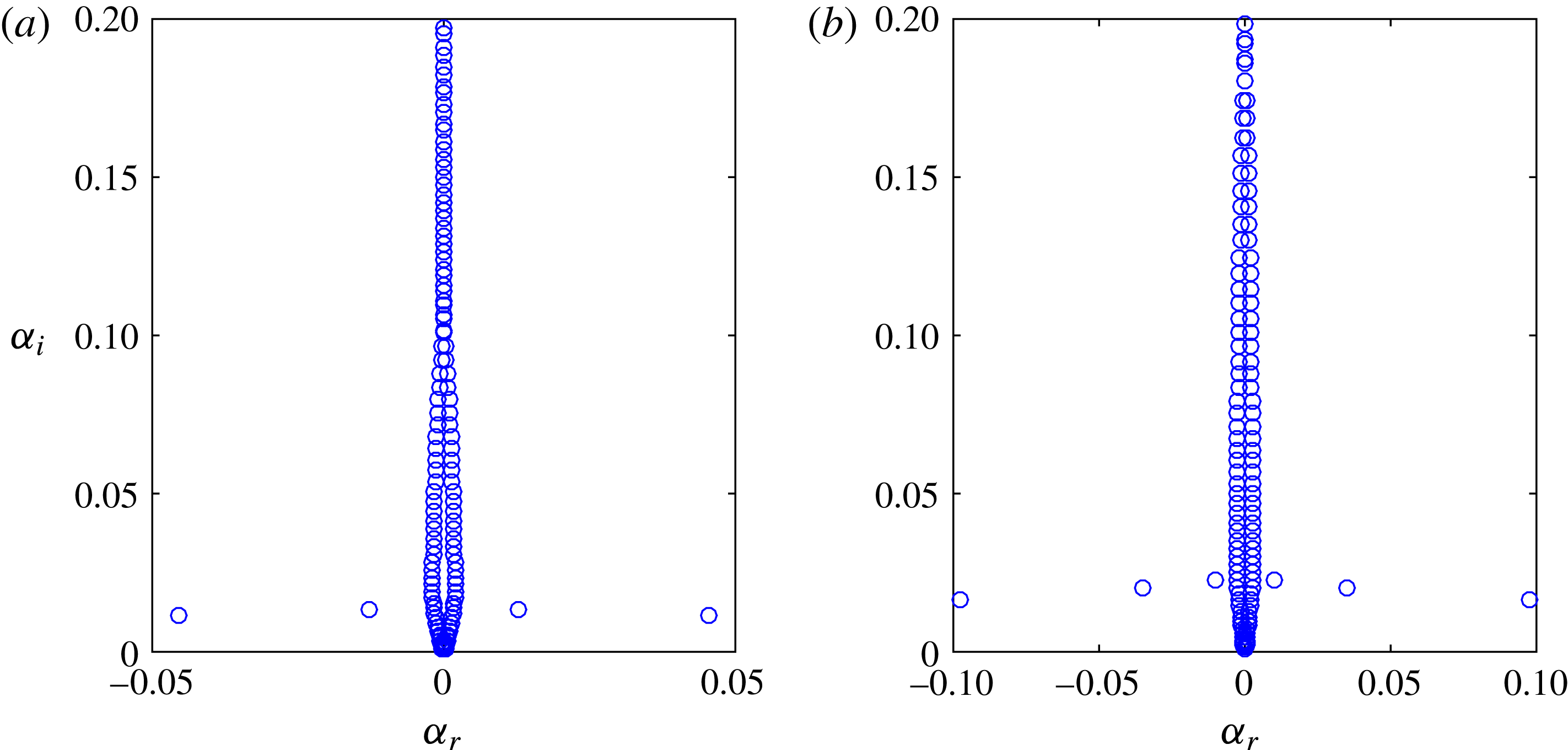
We first examine the eigenvalue spectrum for a representative set of parameters. The eigenvalue spectrum is shown for
 $Re=4200$
,
 $\unicode[STIX]{x1D6FD}=1.85$
,
 $\unicode[STIX]{x1D714}=0$
and
 $\unicode[STIX]{x1D705}=1/500$
in figure 2(a) and
 $\unicode[STIX]{x1D705}=1/125$
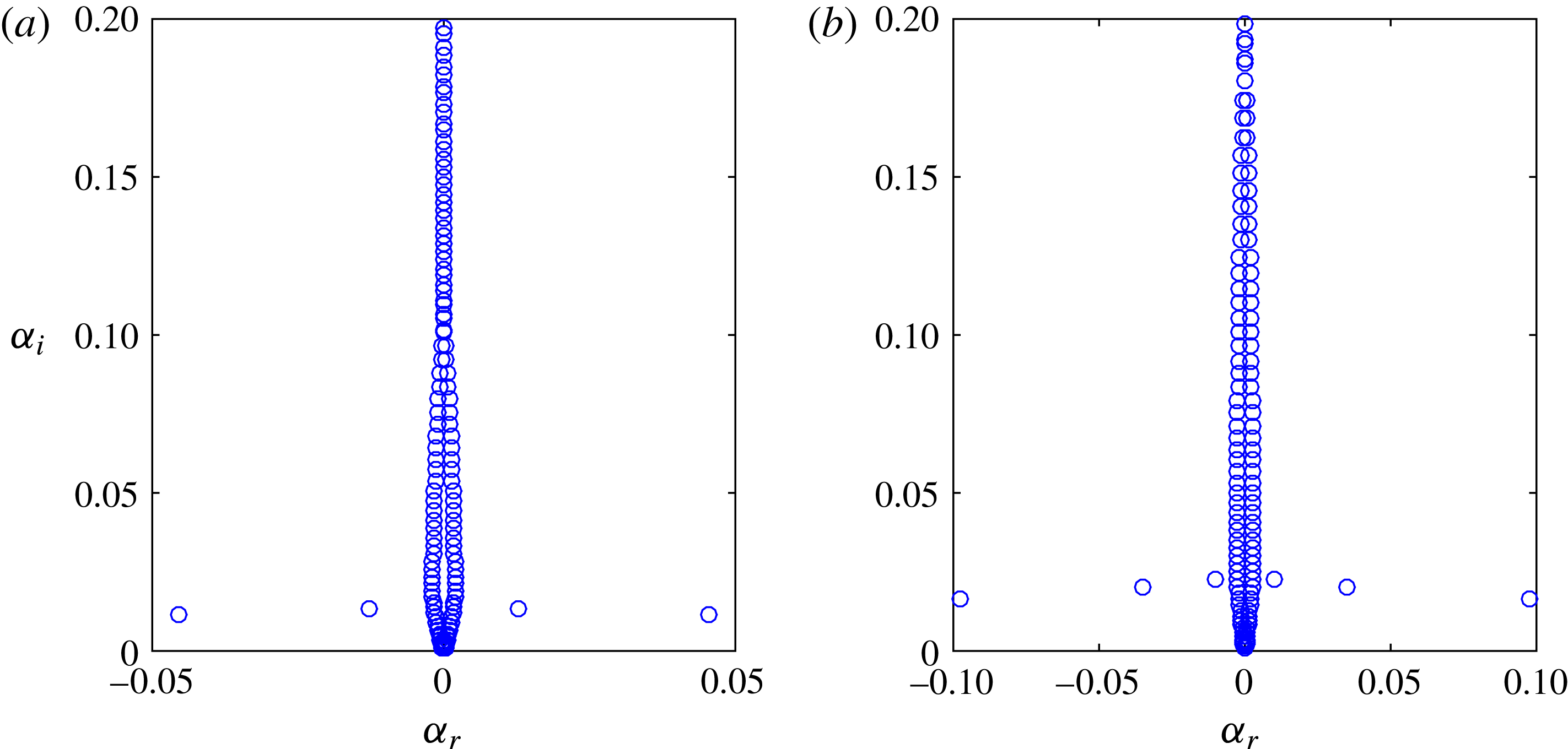
in figure 2(b). As expected, the flow is linearly stable, and as a result of the curvature there are some eigenvalues off the imaginary axis (for a flat plate and
 $\unicode[STIX]{x1D714}=0$
all the eigenvalues lie on the imaginary axis). For
 $\unicode[STIX]{x1D705}=1/500\;(\widetilde{G\ddot{o} }=188)$
there are two pairs significantly farther from the imaginary axis, whereas for
 $\unicode[STIX]{x1D705}=1/125\;(\widetilde{G\ddot{o} }=376)$
there are three pairs. These modes bifurcate from the eigenvalues near the imaginary axis as the curvature is increased. The real part of the eigenvalues that are farthest from the imaginary axis scales approximately with
 $\unicode[STIX]{x1D705}^{1/2}$
.
The eigenvalues for a boundary layer over a convex surface,
 $Re=4200$
,
 $\unicode[STIX]{x1D6FD}=1.85$
and
 $\unicode[STIX]{x1D714}=0$
. (a)
 $\unicode[STIX]{x1D705}=1/500\;(\widetilde{G\ddot{o} }=188)$
. (b)
 $\unicode[STIX]{x1D705}=1/125\;(\widetilde{G\ddot{o} }=376)$
.
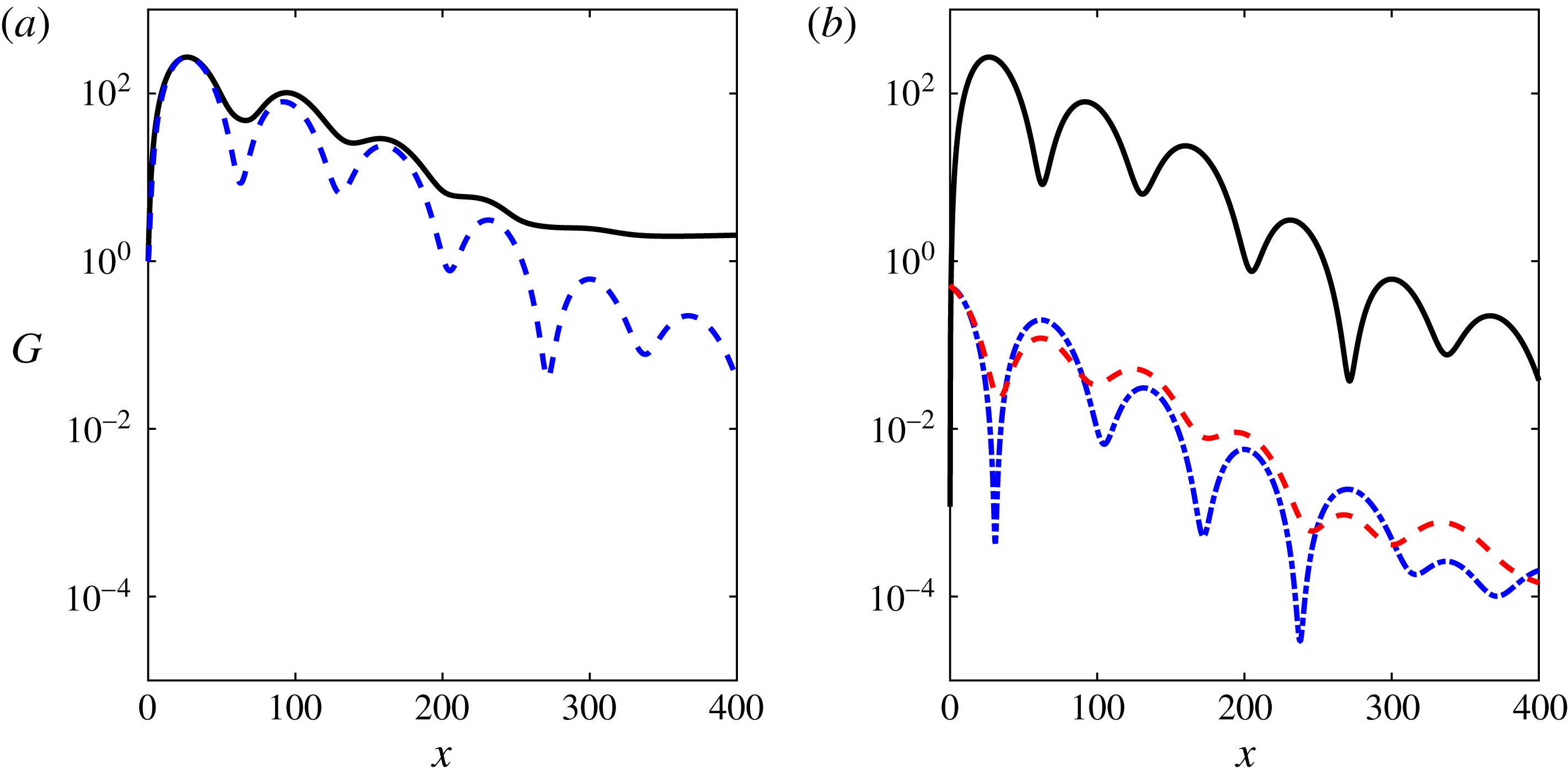
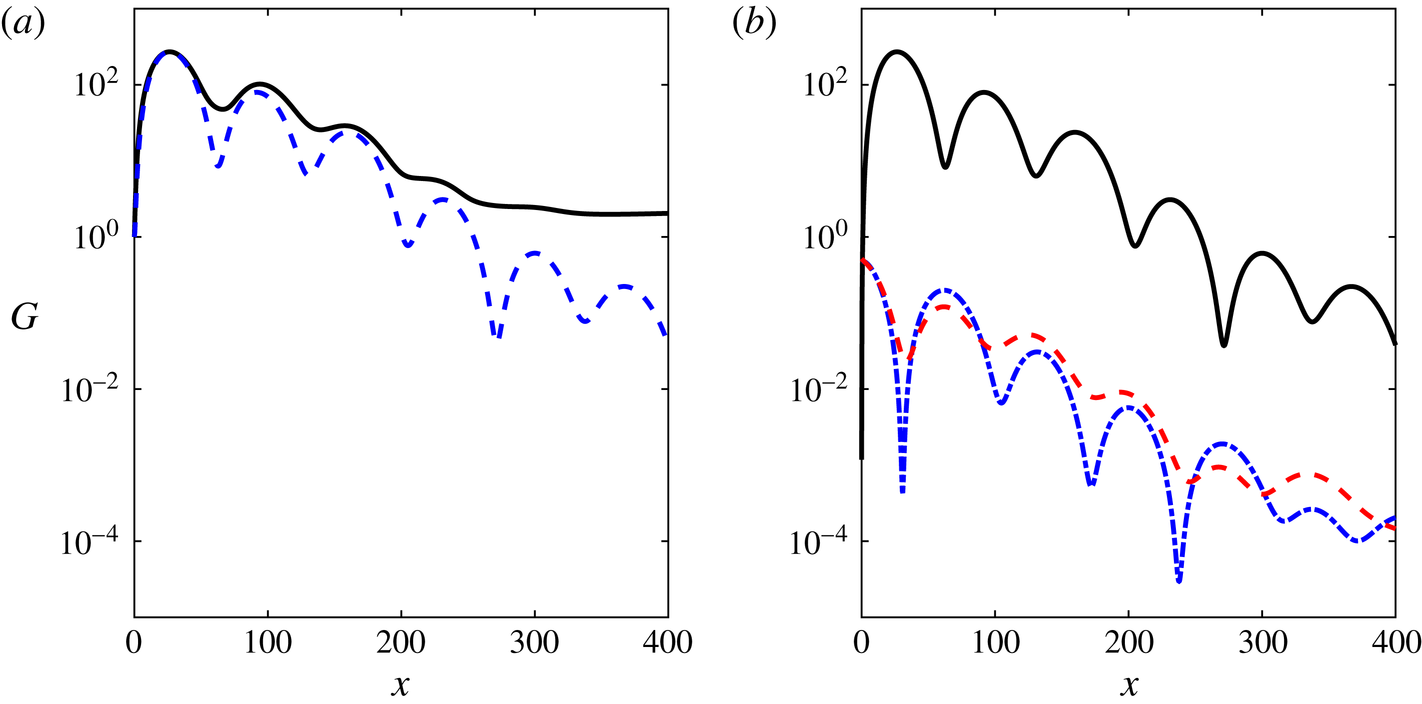
Optimal energy gain for a boundary layer over a convex surface,
 $Re=4200$
,
 $\unicode[STIX]{x1D6FD}=1.85$
,
 $\unicode[STIX]{x1D714}=0$
and
 $\unicode[STIX]{x1D705}=1/500\;(\widetilde{G\ddot{o} }=188)$
. (a) Envelope (solid line) and optimal at
 $x=27$
(dashed line). (b) Energy gain in the velocity components for the disturbance achieving an optimal at
 $x=27$
. The streamwise, wall-normal and spanwise components are marked by solid, dash-dotted and dashed lines, respectively.
The results of a transient growth analysis for the above parameters and
 $\unicode[STIX]{x1D705}=1/500$
(
 $\widetilde{G\ddot{o} }=188$
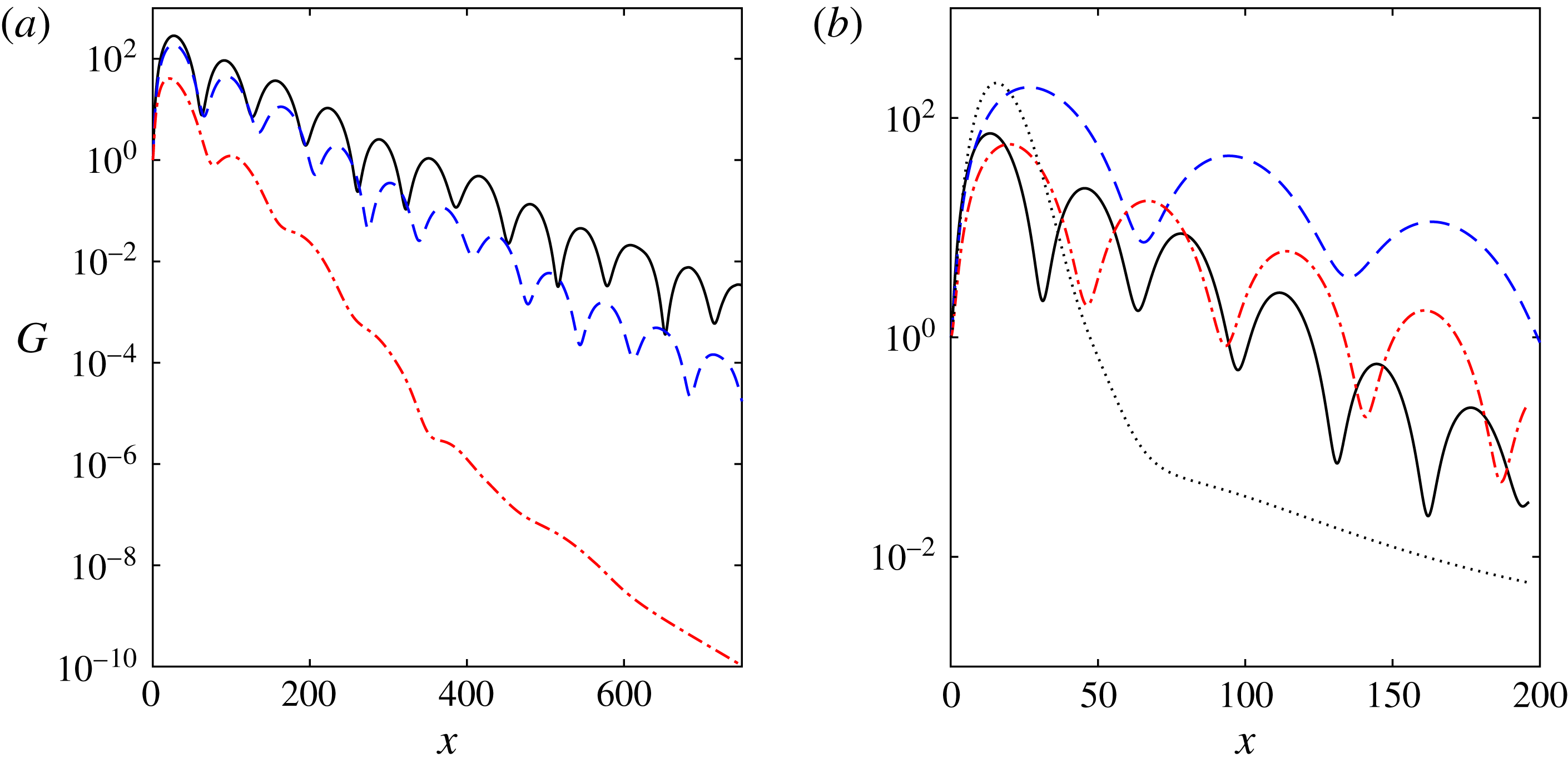
) is presented in figure 3. The envelope of optimal growth and the optimal disturbance achieving maximal growth at
 $x=27$
are indicated by the solid and dashed lines in figure 3(a), respectively. The streamwise, wall-normal and spanwise components of the energy gain for the optimal disturbance are presented in figure 3(b). The envelope and optimal disturbance share similar features of long-wavelength streamwise oscillations. As in other wall-bounded shear flows (e.g. Butler & Farrell Reference Butler and Farrell1992), most of the energy is concentrated in the streamwise component due to the lift-up effect; however, once the streaks reach a considerable magnitude they generate streamwise vortices (rolls) due to the centrifugal force. The secondary streamwise vortices have an opposite sign to the initial streamwise vortices, and these in turn generate streaks with the opposite sign to the previous streaks (as shown in greater detail later). We note that this behaviour contrasts with that observed for concave surfaces, where the streaks intensify the streamwise vortices, leading to the Görtler instability. The process continues with a distinct streamwise wavelength and an almost purely exponential decay of the peaks. The wavelength is related to the real part of the eigenvalues that are farthest from the imaginary axis presented in figure 2(a), and the estimated wavelength is
 $\unicode[STIX]{x1D706}=2\unicode[STIX]{x03C0}/\unicode[STIX]{x1D6FC}_{r}=138$
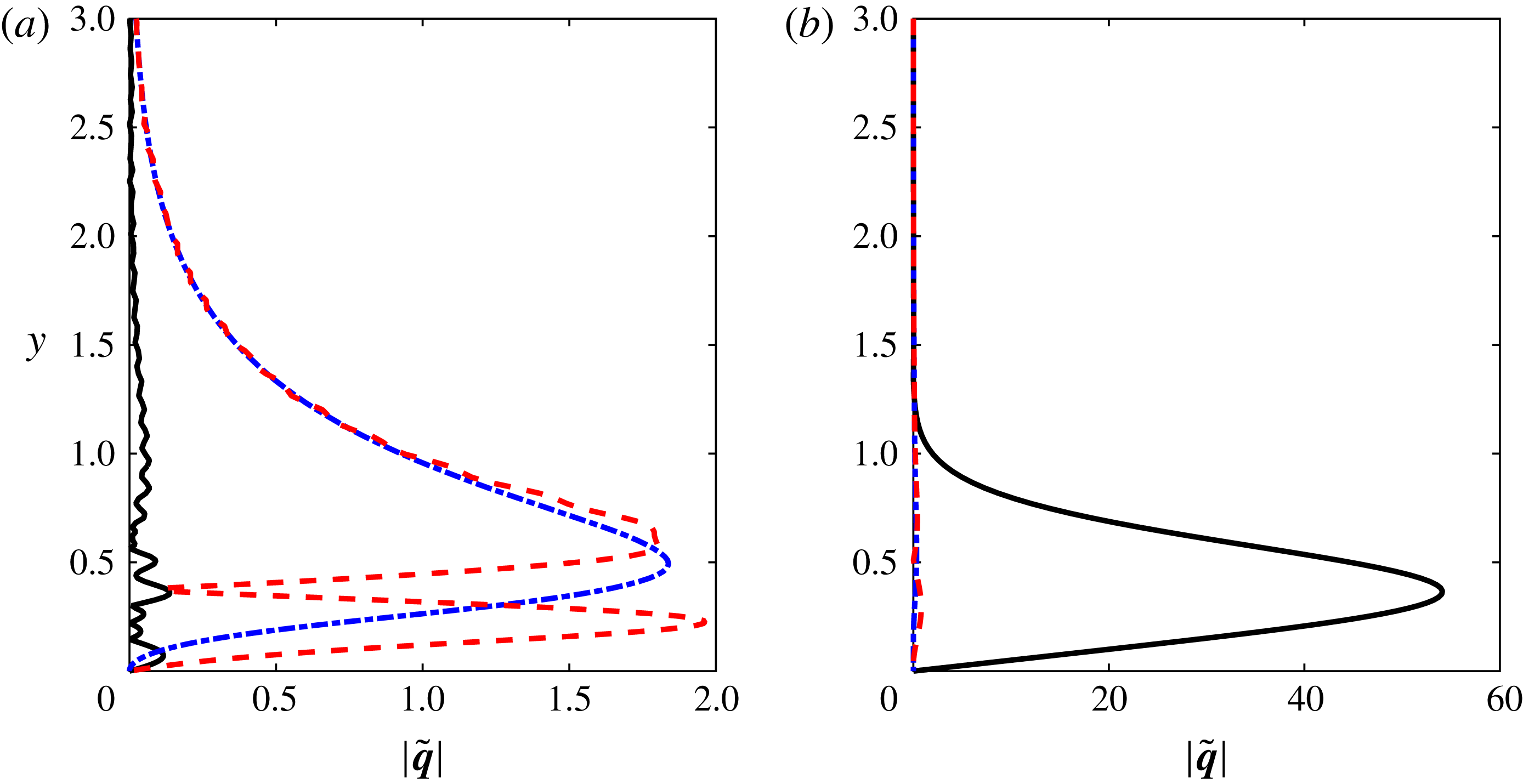
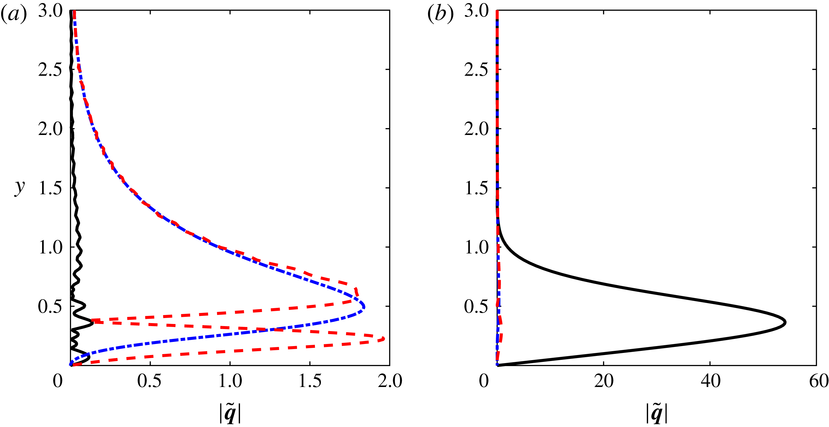
. The velocity components
 $\tilde{\boldsymbol{q}}=(\tilde{u} ,\tilde{v},\tilde{w})^{\text{T}}$
corresponding to the optimal disturbance are shown in figure 4. The inflow condition is presented in figure 4(a). Most of the energy is concentrated in the cross-stream components, which represent a row of counter-rotating vortices. The response of the flow at
 $x=27$
is presented in figure 4(b). Here, most of the energy is in the streamwise component, which is an order of magnitude higher than the cross-stream components at the inflow.
As demonstrated above, the streamwise wavelength of the streaks can be estimated from the real part of the eigenvalues that are farthest from the imaginary axis, which within a reasonable approximation depend linearly on
 $\unicode[STIX]{x1D705}^{1/2}$
. Thus, the wavelength behaves like
 $\unicode[STIX]{x1D706}\sim \unicode[STIX]{x1D705}^{-1/2}$
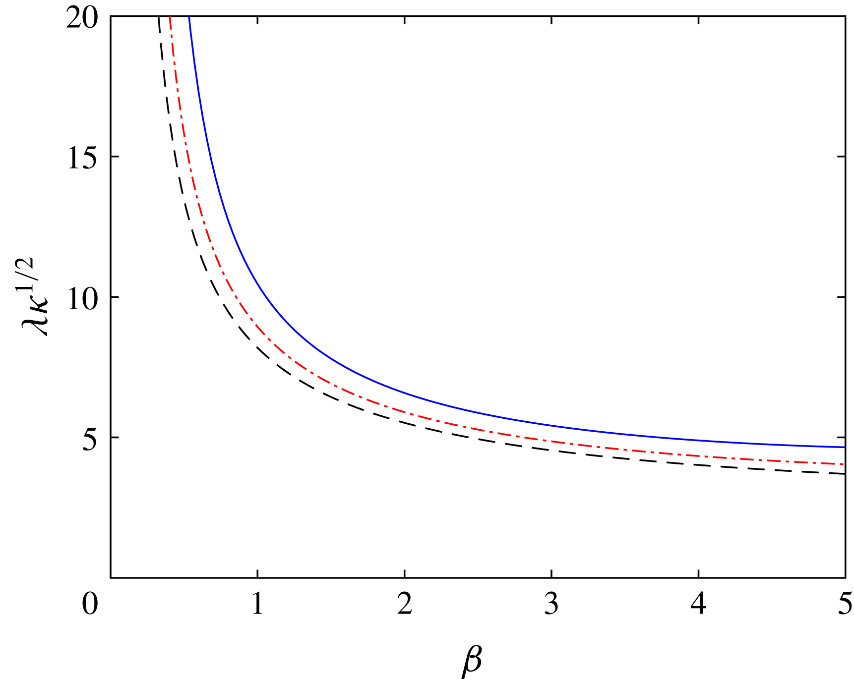
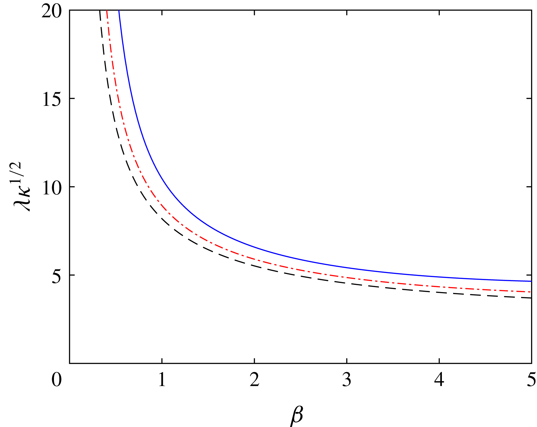
. The dependence of
 $\unicode[STIX]{x1D706}\unicode[STIX]{x1D705}^{1/2}$
on the spanwise wavenumber for several
 $\widetilde{G\ddot{o} }$
is presented in figure 5. The streamwise length of the streaks increases as the spanwise wavenumber decreases. In particular, the results show a minor influence of
 $\widetilde{G\ddot{o} }$
on the wavelength of the streaks.
The velocity components
 $\tilde{\boldsymbol{q}}=(\tilde{u} ,\tilde{v},\tilde{w})^{\text{T}}$
of the optimal disturbance for
 $Re=4200$
,
 $\unicode[STIX]{x1D6FD}=1.85$
,
 $\unicode[STIX]{x1D714}=0$
and
 $\unicode[STIX]{x1D705}=1/500\;(\widetilde{G\ddot{o} }=188)$
. (a) Inflow condition (
 $x=0$
). (b) Response at
 $x=27$
. The streamwise, wall-normal and spanwise components are marked by solid, dash-dotted and dashed lines, respectively.
Estimated streamwise wavelength of the streak versus
 $\unicode[STIX]{x1D6FD}$
. The value of
 $\unicode[STIX]{x1D706}\unicode[STIX]{x1D705}^{1/2}$
is shown for various
 $\widetilde{G\ddot{o} }$
. Solid, dash-dotted and dashed lines represent
 $\widetilde{G\ddot{o} }=100$
, 200 and 400, respectively.
Curvature effects on the optimal energy growth for steady disturbances (
 $\unicode[STIX]{x1D714}=0$
) and various spanwise wavenumbers. (a)
 $G_{max}/Re^{2}\times 10^{4}$
. (b)
 $x(G_{max})/Re\times 10^{2}$
.

3.1 Curvature effect
The effect of the curvature on the transient amplification of disturbances is investigated for steady disturbances (
 $\unicode[STIX]{x1D714}=0$
). It is well known that for planar wall-bounded shear flows, such as flat plate boundary layer and channel flow, the maximum energy growth scales with
 $Re^{2}$
, while the location where it is attained is proportional to
 $Re$
(e.g. Gustavsson Reference Gustavsson1991). Thus, in the following results the energy gain is normalized by
 $Re^{2}$
and the streamwise position by
 $Re$
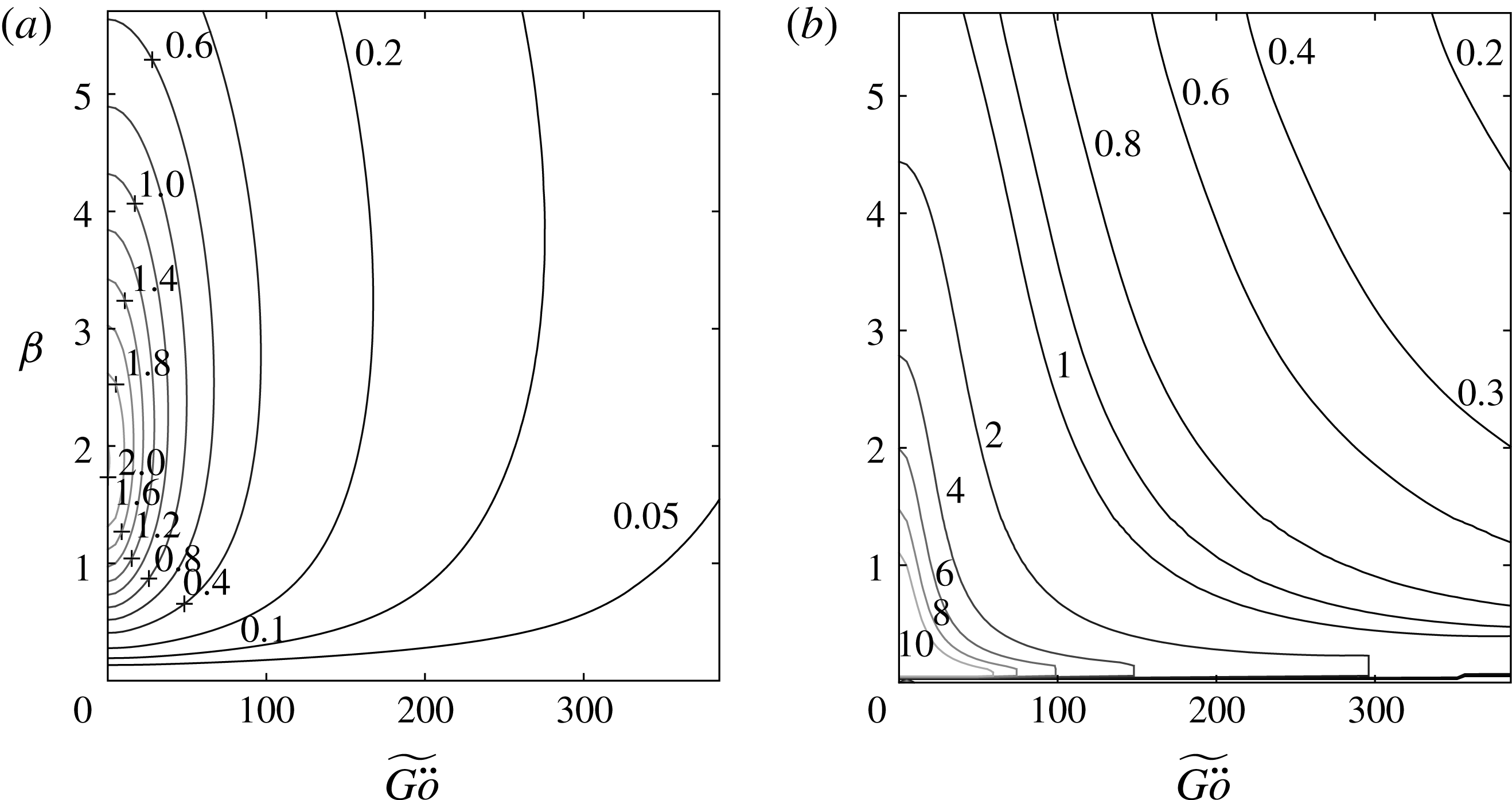
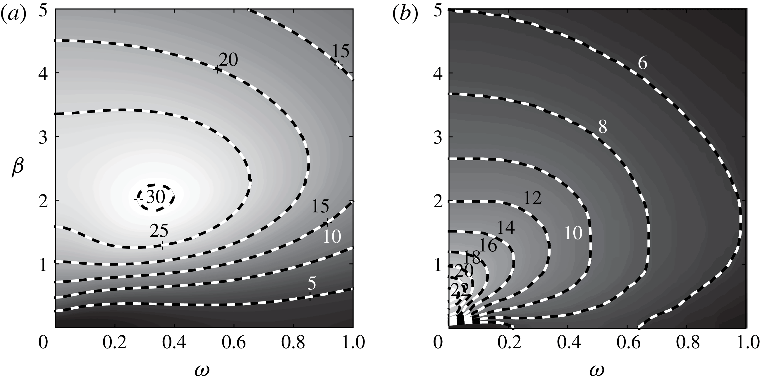
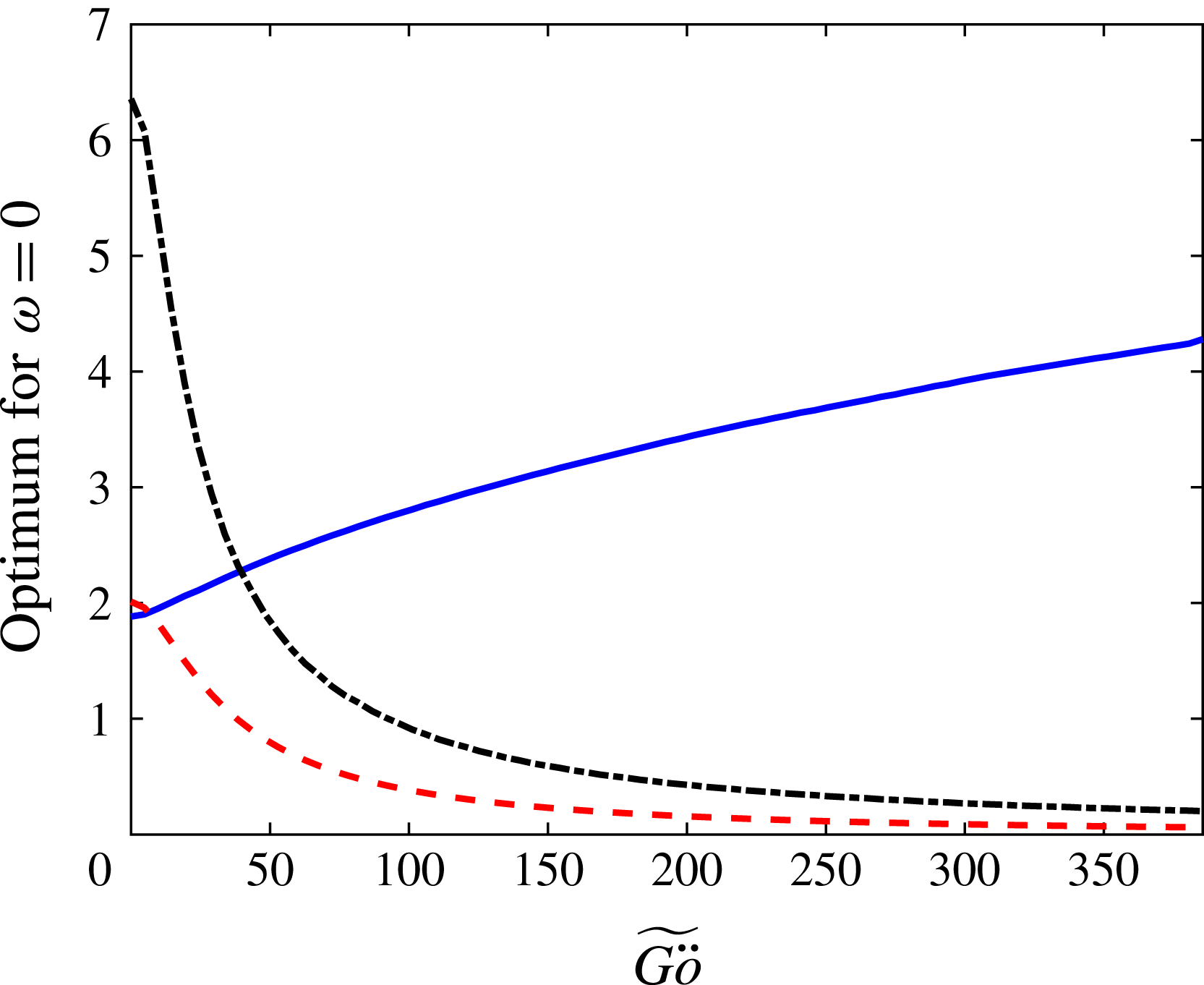
. The effect of the curvature on the optimal growth for various spanwise wavenumbers is presented in figure 6. Higher curvature, and thus higher
 $\widetilde{G\ddot{o} }$
, lead to significant reduction of the optimal energy gain and the location where it is attained. The reduction in the location of the highest perturbation kinetic energy is attributed to the shortening of the streamwise wavelength of the streaks, which behaves like
 $\unicode[STIX]{x1D706}\sim \unicode[STIX]{x1D705}^{-1/2}$
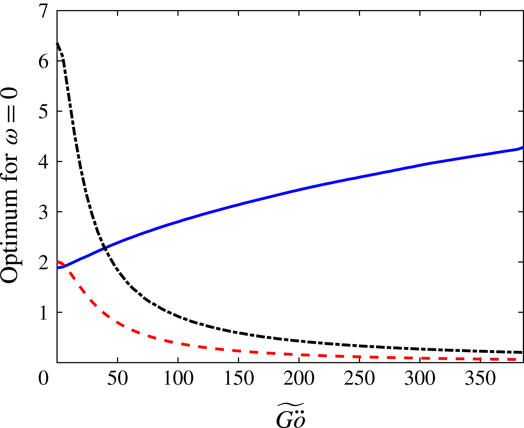
. The optimal spanwise wavenumber, leading to the maximal growth for various curvatures, is presented by the solid line in figure 7, together with the optimal energy amplification ratio (dashed line) and its location (dash-dotted line). The optimal spanwise wavenumber increases with
 $\widetilde{G\ddot{o} }$
, and the figure allows direct comparison between optimal disturbances for various curvatures.
Curvature effects on the optimal energy growth for steady disturbances (
 $\unicode[STIX]{x1D714}=0$
). The optimal spanwise wavenumbers (solid line), optimal growth
 $G_{max}/Re^{2}\times 10^{4}$
(dashed line) and location of optimal growth
 $x(G_{max})/Re\times 10^{2}$
(dash-dotted line).
Optimal energy growth for various frequencies and spanwise wavenumbers,
 $Re=570$
and
 $\unicode[STIX]{x1D705}=0$
. (a)
 $G_{max}$
. (b)
 $x(G_{max})$
.
3.2 Unsteady disturbances
Next, the effect of the frequency,
 $\unicode[STIX]{x1D714}$
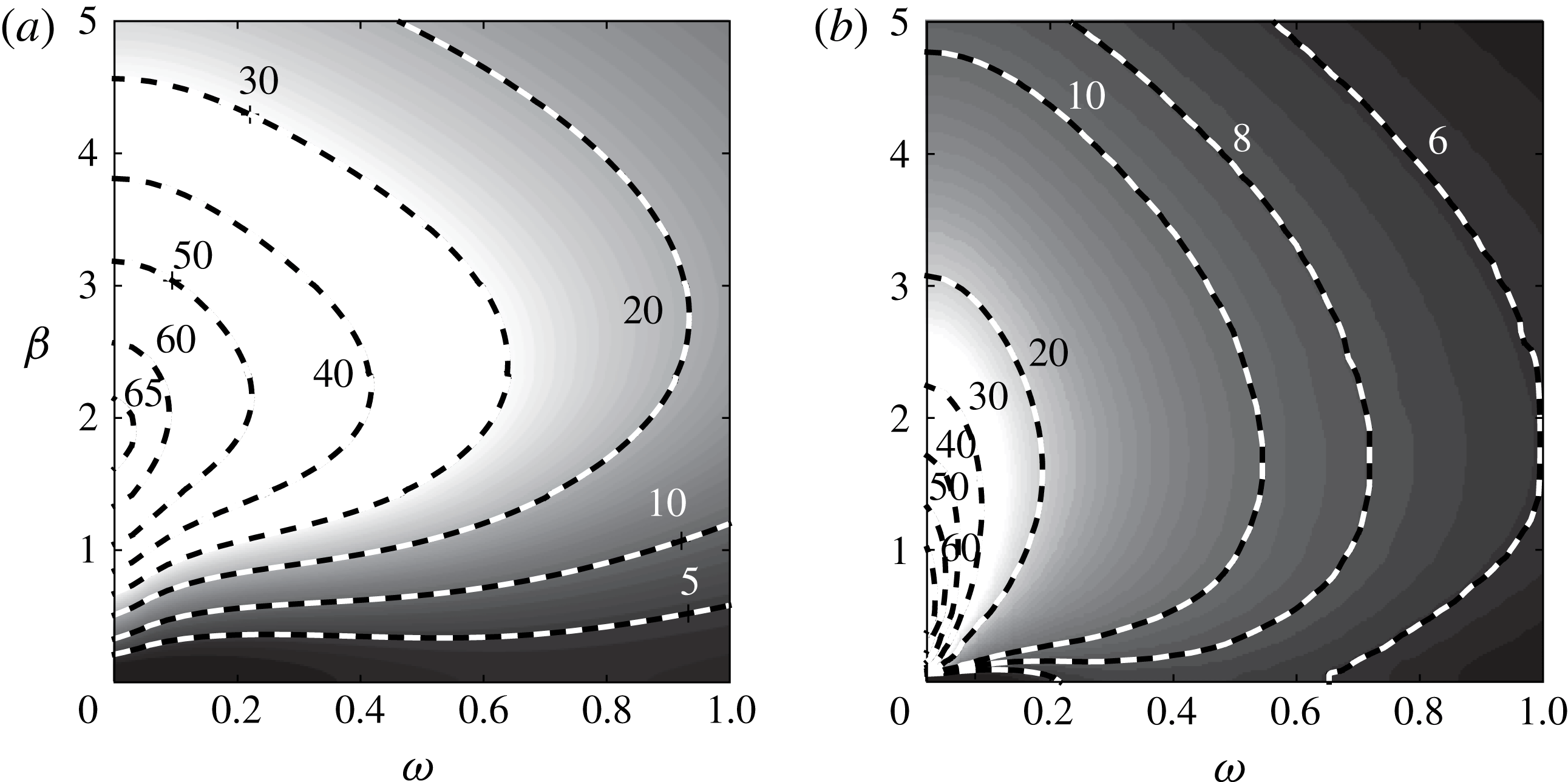
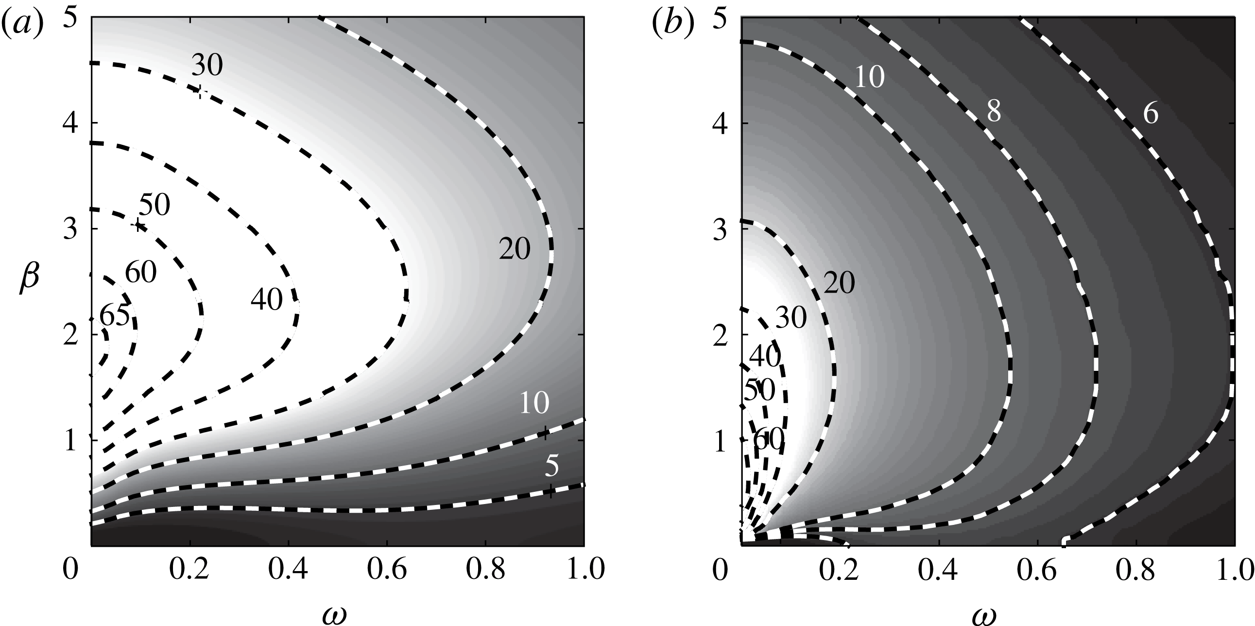
, is analysed. For reference, the optimal energy amplification ratio for a flat plate boundary layer and its location for the parameters
 $Re=570$
and
 $\unicode[STIX]{x1D705}=0$
are shown in figure 8. The optimal growth is obtained for a steady disturbance and
 $\unicode[STIX]{x1D6FD}=1.85$
due to the lift-up effect, which is responsible for the generation of streaks from the vortices. The optimal growth and its location for the parameters
 $Re=570$
and
 $\unicode[STIX]{x1D705}=1/140$
(
 $\widetilde{G\ddot{o} }=48$
) are shown in figure 9. Here, the optimal gain is achieved for an unsteady disturbance as a result of the opposing effects of lift-up and the centrifugal mechanism. The lift-up effect tends to increase the energy amplification as
 $\unicode[STIX]{x1D714}\rightarrow 0$
, while the centrifugal mechanism tends to decrease the growth in that limit.
Optimal energy growth for various frequencies and spanwise wavenumbers,
 $Re=570$
and
 $\unicode[STIX]{x1D705}=1/140$
(
 $\widetilde{G\ddot{o} }=48$
). (a)
 $G_{max}$
. (b)
 $x(G_{max})$
.

The centrifugal mechanism causes a reduction of the optimal growth from
 ${\sim}65$
to
 ${\sim}25$
for
 $\unicode[STIX]{x1D714}=0$
and
 $\unicode[STIX]{x1D6FD}=1.85$
, and a reduction from
 ${\sim}40$
to
 ${\sim}30$
for
 $\unicode[STIX]{x1D714}=0.34$
and
 $\unicode[STIX]{x1D6FD}=1.85$
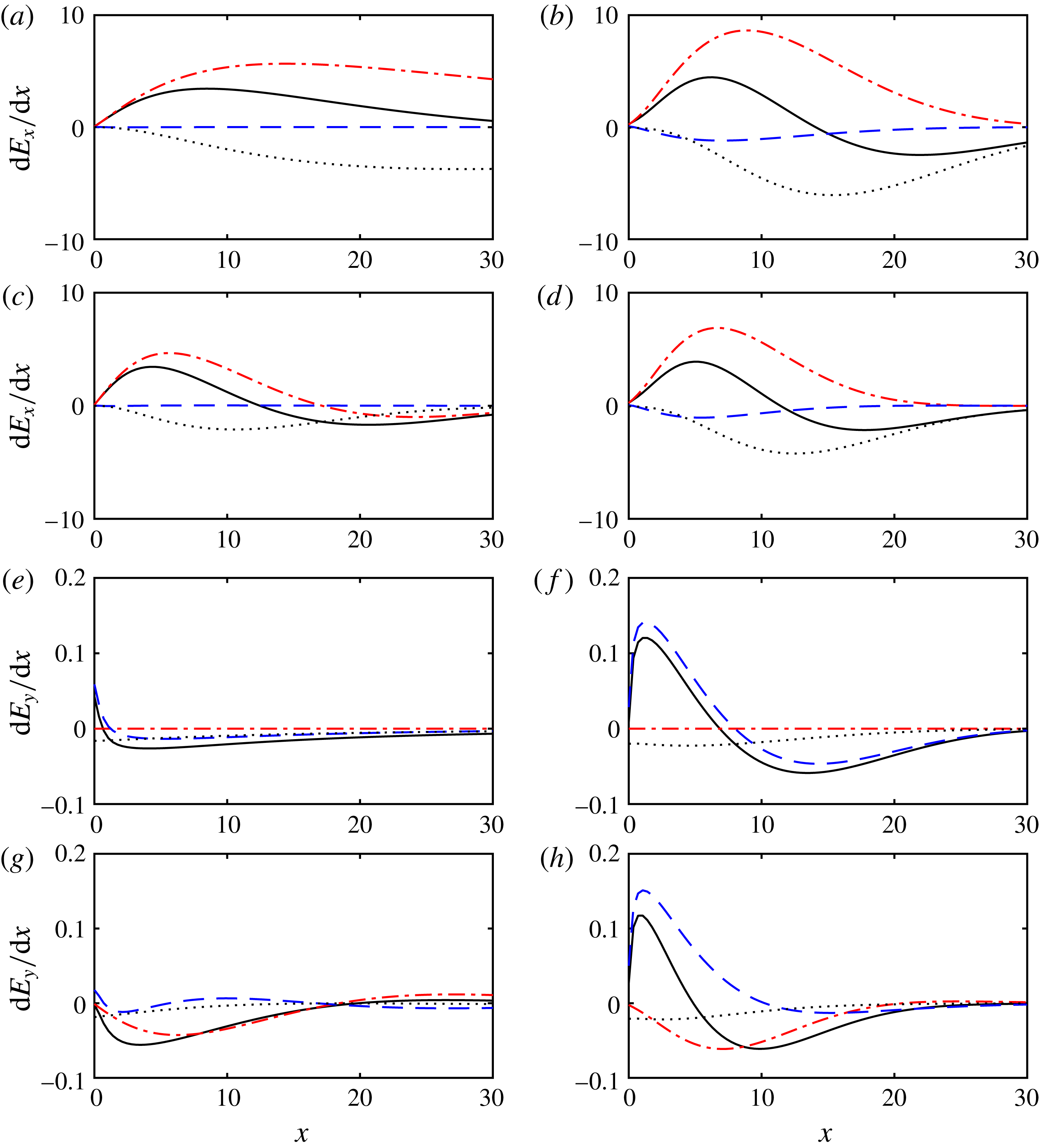
. To further clarify the underlying mechanism behind the reduction in growth, an energy production–dissipation analysis is performed (cf. e.g. Hack & Zaki Reference Hack and Zaki2015). For a parallel flow over a curved surface, the equations governing the evolution of the kinetic energy components are
 $$\begin{eqnarray}\displaystyle & \displaystyle \frac{\text{d}E_{x}}{\,\text{d}x}=\int _{0}^{\infty }\tilde{u} \frac{\unicode[STIX]{x2202}\tilde{u} }{\unicode[STIX]{x2202}x}\,\text{d}y=\underbrace{-\int _{0}^{\infty }\frac{U_{B}^{\prime }}{U_{B}}\tilde{u} \tilde{v}\,\text{d}y}_{P_{x}}\underbrace{-\int _{0}^{\infty }\frac{\tilde{u} }{U_{B}}\frac{\unicode[STIX]{x2202}\tilde{p}}{\unicode[STIX]{x2202}x}\,\text{d}y}_{R_{x}}\underbrace{+\frac{1}{Re}\int _{0}^{\infty }\frac{\tilde{u} \unicode[STIX]{x1D6FB}^{2}\tilde{u} }{U_{B}}\,\text{d}y}_{D_{x}},\qquad & \displaystyle\end{eqnarray}$$
 $$\begin{eqnarray}\displaystyle & \displaystyle \frac{\text{d}E_{y}}{\,\text{d}x}=\int _{0}^{\infty }\tilde{v}\frac{\unicode[STIX]{x2202}\tilde{v}}{\unicode[STIX]{x2202}x}\,\text{d}y=\underbrace{\int _{0}^{\infty }2\unicode[STIX]{x1D705}\tilde{u} \tilde{v}\,\text{d}y}_{P_{y}}\underbrace{-\int _{0}^{\infty }\frac{\tilde{v}}{U_{B}}\frac{\unicode[STIX]{x2202}\tilde{p}}{\unicode[STIX]{x2202}y}\,\text{d}y}_{R_{y}}\underbrace{+\frac{1}{Re}\int _{0}^{\infty }\frac{\tilde{v}\unicode[STIX]{x1D6FB}^{2}\tilde{v}}{U_{B}}\,\text{d}y}_{D_{y}}, & \displaystyle\end{eqnarray}$$
 $$\begin{eqnarray}\displaystyle & \displaystyle \frac{\text{d}E_{z}}{\,\text{d}x}=\int _{0}^{\infty }\tilde{w}\frac{\unicode[STIX]{x2202}\tilde{w}}{\unicode[STIX]{x2202}x}\,\text{d}y=\underbrace{-\int _{0}^{\infty }\frac{\tilde{w}}{U_{B}}\frac{\unicode[STIX]{x2202}\tilde{p}}{\unicode[STIX]{x2202}z}\,\text{d}y}_{R_{z}}\underbrace{+\frac{1}{Re}\int _{0}^{\infty }\frac{\tilde{w}\unicode[STIX]{x1D6FB}^{2}\tilde{w}}{U_{B}}\,\text{d}y}_{D_{z}}, & \displaystyle\end{eqnarray}$$
Energy balance for the kinetic energy of the streamwise (a–d) and wall-normal (e–h) velocity components for
 $Re=570$
and
 $\unicode[STIX]{x1D6FD}=1.85$
. Production,
 $P$
(dash-dotted line), pressure redistribution,
 $R$
(dashed line), dissipation,
 $D$
(dotted line), and the sum of the three terms (solid line). (a,e)
 $\unicode[STIX]{x1D705}=0$
and
 $\unicode[STIX]{x1D714}=0$
. (b,f)
 $\unicode[STIX]{x1D705}=0$
and
 $\unicode[STIX]{x1D714}=0.34$
. (c,g)
 $\unicode[STIX]{x1D705}=1/140$
and
 $\unicode[STIX]{x1D714}=0$
. (d,h)
 $\unicode[STIX]{x1D705}=1/140$
and
 $\unicode[STIX]{x1D714}=0.34$
.

Figure 10 shows a comparison between the following four cases:
 $\unicode[STIX]{x1D705}=0$
and
 $\unicode[STIX]{x1D714}=0$
(figure 10
a,e);
 $\unicode[STIX]{x1D705}=0$
and
 $\unicode[STIX]{x1D714}=0.34$
(figure 10
b,f);
 $\unicode[STIX]{x1D705}=1/140$
and
 $\unicode[STIX]{x1D714}=0$
(figure 10
c,g);
 $\unicode[STIX]{x1D705}=1/140$
and
 $\unicode[STIX]{x1D714}=0.34$
(figure 10
d,h). The energy balance of the streamwise component is shown in figure 10(a–d), and that of the wall-normal component in figure 10(e–h). The production terms are indicated by the dash-dotted curves, the pressure redistribution by the dashed curves and the dissipation by the dotted curves. A comparison between figures 10(a) and 10(b) reveals the effect of the frequency for a flat plate: the production
 $P_{x}$
as well as the dissipation
 $D_{x}$
intensify, which results in a higher peak of the total change of
 $E_{x}$
; however, the location of maximal growth (
 $\text{d}E_{x}/\,\text{d}x=0$
) decreases rapidly, from
 ${\sim}30$
to
 ${\sim}15$
, which leads to a lower peak of the energy gain. A comparison between figures 10(e) and 10(f) reveals that the rate of change of
 $E_{y}$
is governed mostly by the pressure redistribution
 $R_{y}$
. A comparison between figures 10(a,c) and 10(e,g) allows the assessment of the effect of the curvature for a steady disturbance. A significant reduction in
 $P_{x}$
is observed, resulting from the negative production
 $P_{y}$
attributed to the convex curvature (figure 10
g), which decreases the wall-normal component in
 $P_{x}$
. A comparison between figures 10(b,d) and 10(f,h) enables an analysis of the curvature effect for
 $\unicode[STIX]{x1D714}=0.34$
. As in the steady case considered above, negative
 $P_{y}$
leads to a reduction of the wall-normal component, which in turn causes a reduction of
 $P_{x}$
; however, this effect is substantially less significant than in the steady case. Finally, a comparison between figures 10(c,d) and 10(g,h) enables the evaluation of the effect of the frequency for a convex curvature. As for the flat plate, the rate of
 $E_{y}$
is governed mostly by
 $R_{y}$
, even in the presence of a negative
 $P_{y}$
resulting from the curvature. This leads to growth of the wall-normal component for
 $\unicode[STIX]{x1D714}=0.34$
, resulting in higher production
 $P_{x}$
compared to the steady case.
4 DNS of primary disturbances
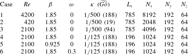
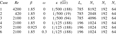
Nonlinear DNS of the full Navier–Stokes equations are conducted to substantiate the results from linear theory. The investigated scenarios are summarized in table 1. A spanwise wavenumber of
 $\unicode[STIX]{x1D6FD}=1.85$
was selected for most simulations since it yields optimal growth for the flat plate boundary layer. The optimal disturbance calculated using the local stability theory (LST) is injected at the inlet. Initially, the linear evolution of the streaks in a non-parallel boundary layer is investigated by setting the amplitude of the streamwise vortices (
 $\max \{\tilde{v}(0,y),\tilde{w}(0,y)\}$
) to
 $10^{-4}$
. Later on, the effects of nonlinearity are investigated by varying
 $E_{0}$
.
Summary of parameters used in the DNS for primary disturbances.
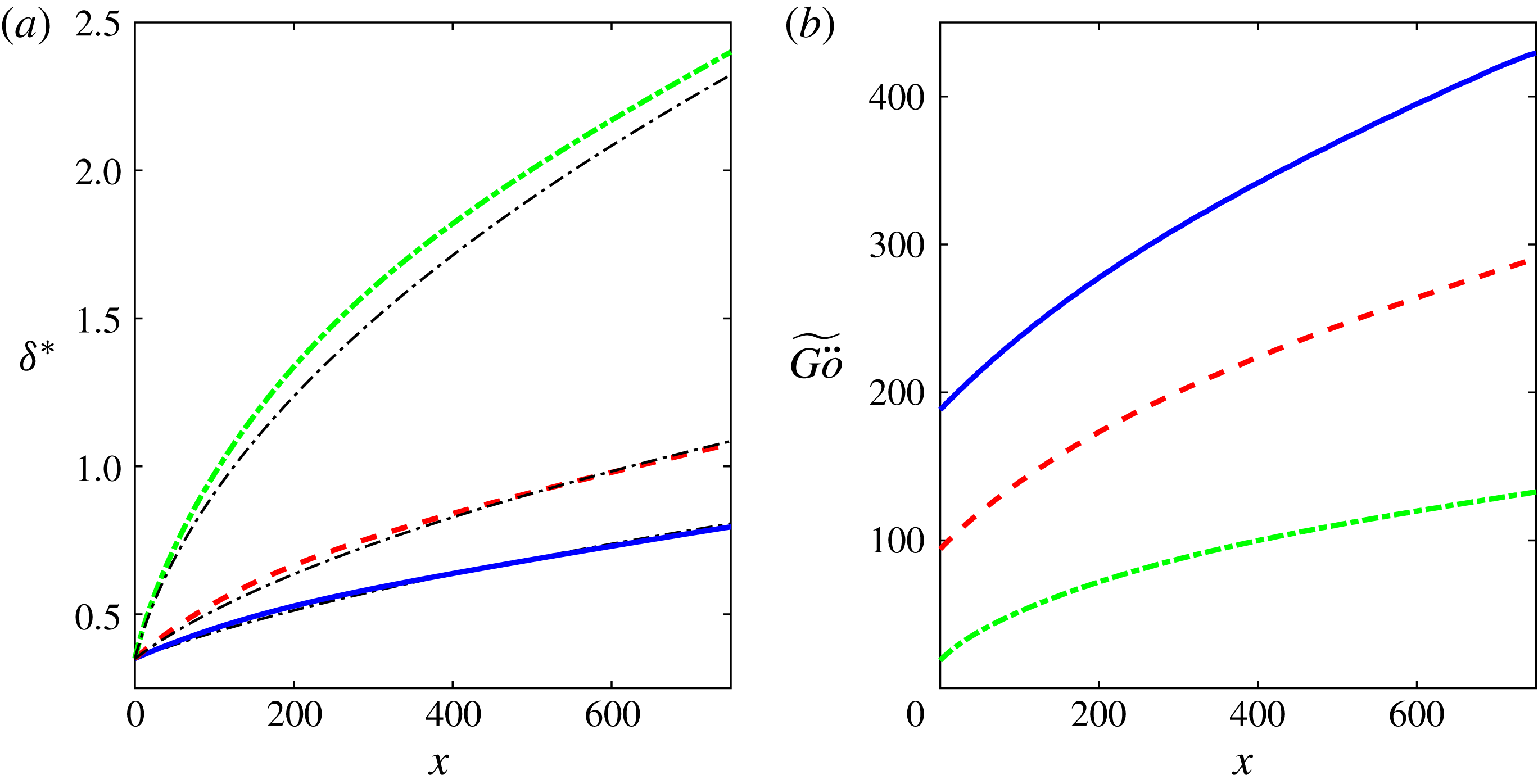
The displacement thickness for cases 1–3, compared to the corresponding values for the flat plate, is shown in figure 11(a). The effect of the curvature is a slight thickening of the boundary layer, which becomes more prominent for lower
 $Re$
. The corresponding Görtler number is presented in figure 11(b), where significant growth of
 $\widetilde{G\ddot{o} }$
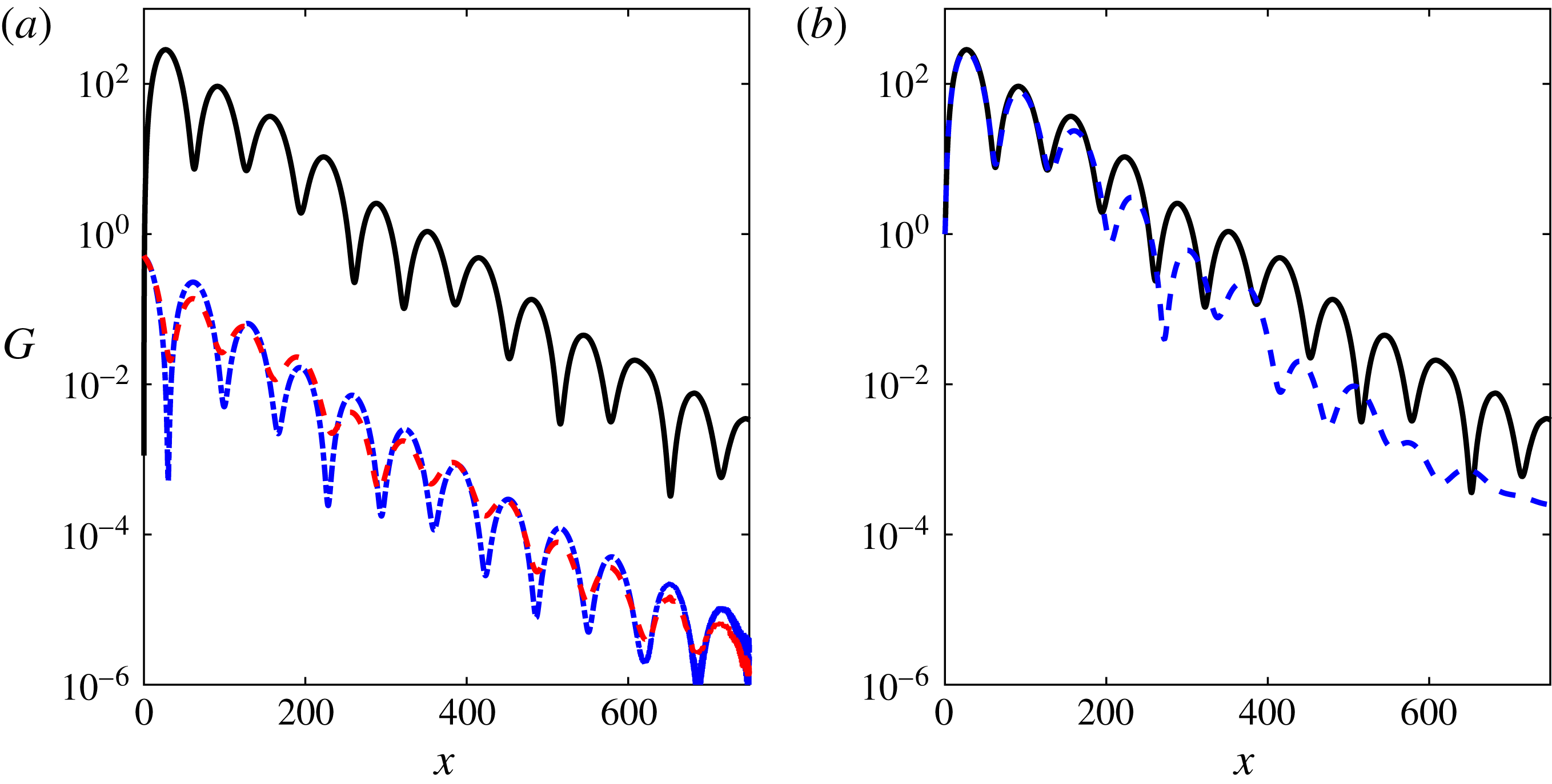
is observed due to the thickening of the boundary layer. Suitable variation of the curvature of the surface allows a constant Görtler number as will be discussed in § 7. The energy growth for case 1 is shown in figure 12. The energy gain in the velocity components is shown in figure 12(a) and a comparison between DNS and LST for the total energy gain is presented in figure 12(b). The mechanism identified by the local stability analysis is manifested in the DNS. The agreement between DNS and linear theory is initially very good and deteriorates at large streamwise locations. To improve the predictions of the LST the effect of adding higher-order terms as a result of the curvature to the equations has been examined as detailed in appendix A. It is found that the LST results remain effectively unchanged.
Displacement thickness and Görtler number for cases 1–3 in table 1. Cases 1, 2 and 3 are marked by solid, dash-dotted and dashed thick lines, respectively. (a) Displacement thickness, the corresponding values for a flat plate are given for reference by the thin dash-dotted lines. (b) Görtler number.

Energy gain for case 1 in table 1. (a) Energy gain in the velocity components. The streamwise, wall-normal and spanwise components are marked by solid, dash-dotted and dashed lines, respectively. (b) Comparison between DNS (solid line) and theory (dashed line).

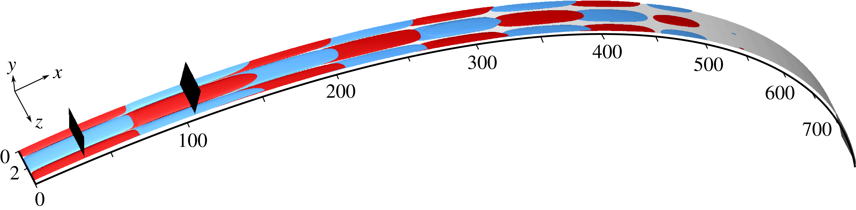
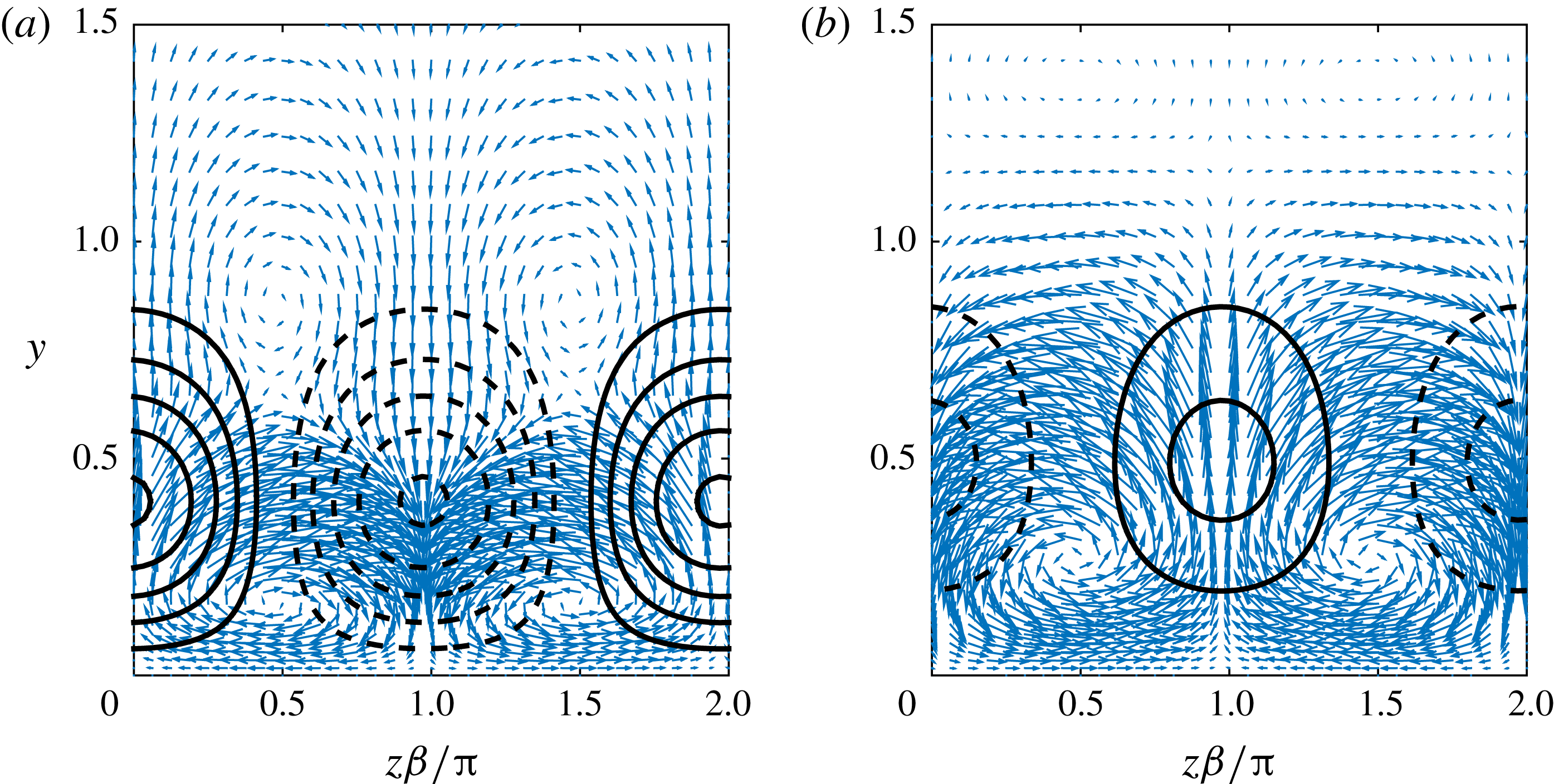
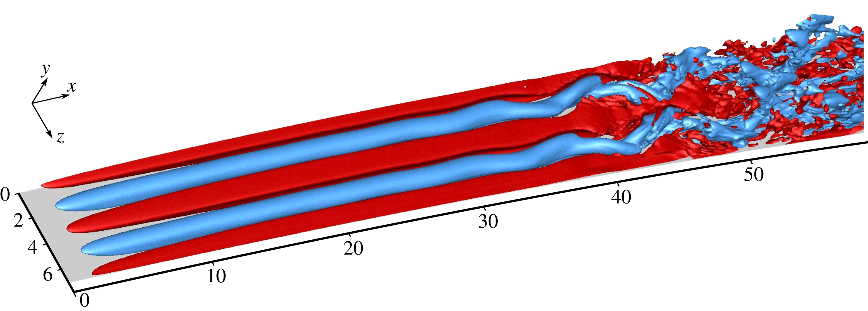
The streaks obtained in the DNS are visualized by isosurfaces of the disturbance streamwise velocity. The streaks for case 1 are shown in figure 13; red (blue) represents positive (negative) isosurfaces of 1 % of the maximum streamwise disturbance velocity. The streaks alternate between positive and negative magnitude and ultimately decay downstream. The velocity components in two cross-stream planes at
 $x=33$
and
 $x=105$
, indicated in figure 13, are presented in figure 14. Since the amplitudes of the streamwise vortices are chosen to represent linear streaks, the velocity components obtained from the DNS are normalized to an inflow energy of 1, i.e.
 $E(x=0)=1$
. The streamwise velocity is represented by equidistant contours (solid, positive; dashed, negative) with intervals of 10, and the cross-stream components are shown by the arrows. The streaks change their direction from
 $x=33$
(figure 14
a) to
 $x=105$
(figure 14
b), and so do the pair of vortices adjacent to the wall. For both cases the vortices work against the streaks as they lift low-speed flow away from the wall at the locations of the positive streaks and push high-speed flow toward the wall at the locations of the negative streaks. A side view of the disturbance streamwise velocity at
 $z=0$
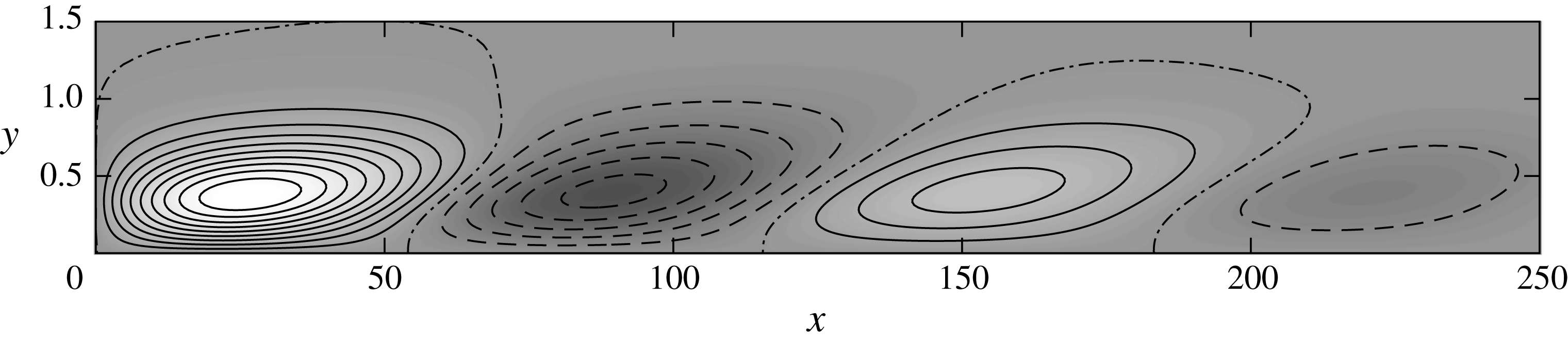
is shown in figure 15, where the curved grid is projected into rectangular coordinates. The disturbance streamwise velocity is normalized by its maximal value, solid (dashed) contours with spacing 0.1 correspond to positive (negative) values while zero perturbation is given by the dash-dotted contour. The maxima of the streaks are obtained around
 $y=0.4$
, every streak achieving a lower magnitude than the previous one, as anticipated from the energy gain shown in figure 12(b). Each set of streaks forms below its predecessor, with an overlap of
 ${\sim}15$
along the streamwise direction.
Streamwise streaks for case 1 in table 1, visualized by isosurfaces of 1 % of the maximum streamwise disturbance velocity (positive, red; negative, blue). Flow from left to right. The two black planes indicate
 $x=33$
(left) and
 $x=105$
(right).

Velocity components of a cross-stream at (a)
 $x=33$
and (b)
 $x=105$
for case 1 in table 1. Solid (dashed) contours represent positive (negative) streamwise velocity with equidistant intervals. Arrows represent the cross-stream components with maximal magnitude of 0.63 (a) and 0.65 (b). The velocity components are normalized to have an inflow energy of 1 at
 $x=0$
.

Streamwise disturbance velocity at
 $z=0$
for case 1 in table 1. The actual grid is projected into rectangular coordinates. Solid (dashed) contours correspond to positive (negative) normalized velocity, with equidistant spacing of 0.1, and dash-dotted contours indicate zero velocity perturbation.

The effect of various parameters on the evolution of the perturbations is presented in figure 16, which shows the energy gain in cases 1–6. The influence of
 $Re$
is shown in figure 16(a) by comparing cases 1–3. All three cases have a similar streamwise wavelength while the decay rate decreases for higher
 $Re$
. A comparison of cases 3–6 is shown in figure 16(b). Increasing the radius by a factor of 4 from
 $R=125$
(case 4, indicated by the solid line) to
 $R=500$
(case 3, indicated by the dashed line) results in doubling of the wavelength, which confirms the scaling
 $\unicode[STIX]{x1D706}\sim \unicode[STIX]{x1D705}^{-1/2}$
found with linear theory. Decreasing the spanwise wavenumber by half (case 5, indicated by the dash-dotted line) results in an increase of the streamwise wavelength relative to case 4 (indicated by the solid line). Setting the frequency to
 $\unicode[STIX]{x1D714}=0.3$
(case 6, indicated by the dotted line) yields a higher gain compared to
 $\unicode[STIX]{x1D714}=0$
(case 4, indicated by the solid line), confirming the LST prediction of unsteady disturbances achieving higher gains than steady disturbances.
Comparison between the energy gain in different cases in table 1. (a) Effect of
 $Re$
: the lines correspond to cases 1 (solid,
 $Re=4200$
), 2 (dash-dotted,
 $Re=420$
) and 3 (dashed,
 $Re=2100$
). (b) Effect of
 $\unicode[STIX]{x1D6FD}$
,
 $\unicode[STIX]{x1D714}$
and
 $\unicode[STIX]{x1D705}$
: the lines represent cases 3 (dashed,
 $\unicode[STIX]{x1D6FD}=1.85$
,
 $\unicode[STIX]{x1D714}=0$
,
 $\unicode[STIX]{x1D705}=1/500$
), 4 (solid,
 $\unicode[STIX]{x1D6FD}=1.85$
,
 $\unicode[STIX]{x1D714}=0$
,
 $\unicode[STIX]{x1D705}=1/125$
), 5 (dash-dotted,
 $\unicode[STIX]{x1D6FD}=0.925$
,
 $\unicode[STIX]{x1D714}=0$
,
 $\unicode[STIX]{x1D705}=1/125$
) and 6 (dotted,
 $\unicode[STIX]{x1D6FD}=1.85$
,
 $\unicode[STIX]{x1D714}=0.3$
,
 $\unicode[STIX]{x1D705}=1/125$
).

So far, we have focused on the evolution of linear streaks. The effect of nonlinearity is evaluated by varying
 $E_{0}$
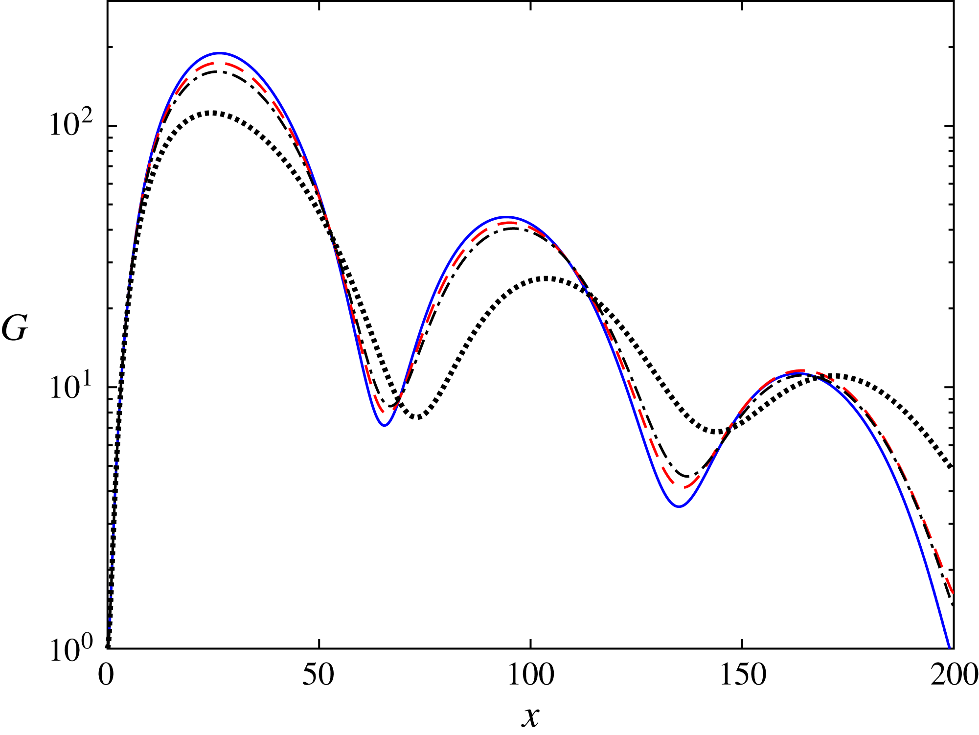
for case 3 in table 1. The energy gain for initial energies of
 $10^{-8}$
,
 $5\times 10^{-5}$
,
 $10^{-4}$
and
 $4\times 10^{-4}$
is shown in figure 17. The nonlinearity decreases the maximal gain as known for planar wall-bounded shear flows. Another effect is an increase in the length of the first streak, which is most noticeable for the highest
 $E_{0}$
.
Effect of nonlinearity on the evolution of the energy gain. Energy gain for case 3 in table 1, for initial energies of
 $10^{-8}$
(solid line),
 $5\times 10^{-5}$
(dashed line),
 $10^{-4}$
(dash-dotted line) and
 $4\times 10^{-4}$
(dotted line).

Fourier components of the streamwise velocity for case 3 in table 1, for initial energies of
 $10^{-8}$
(solid line),
 $5\times 10^{-5}$
(dashed line),
 $10^{-4}$
(dash-dotted line) and
 $4\times 10^{-4}$
(dotted line). The velocities are extracted at the locations of maximal gain.

5 Secondary stability analysis
In the following we investigate the amplification of secondary instabilities in the flow modulated by the streaks. The secondary stability analysis assumes parallel flow and the
 $x$
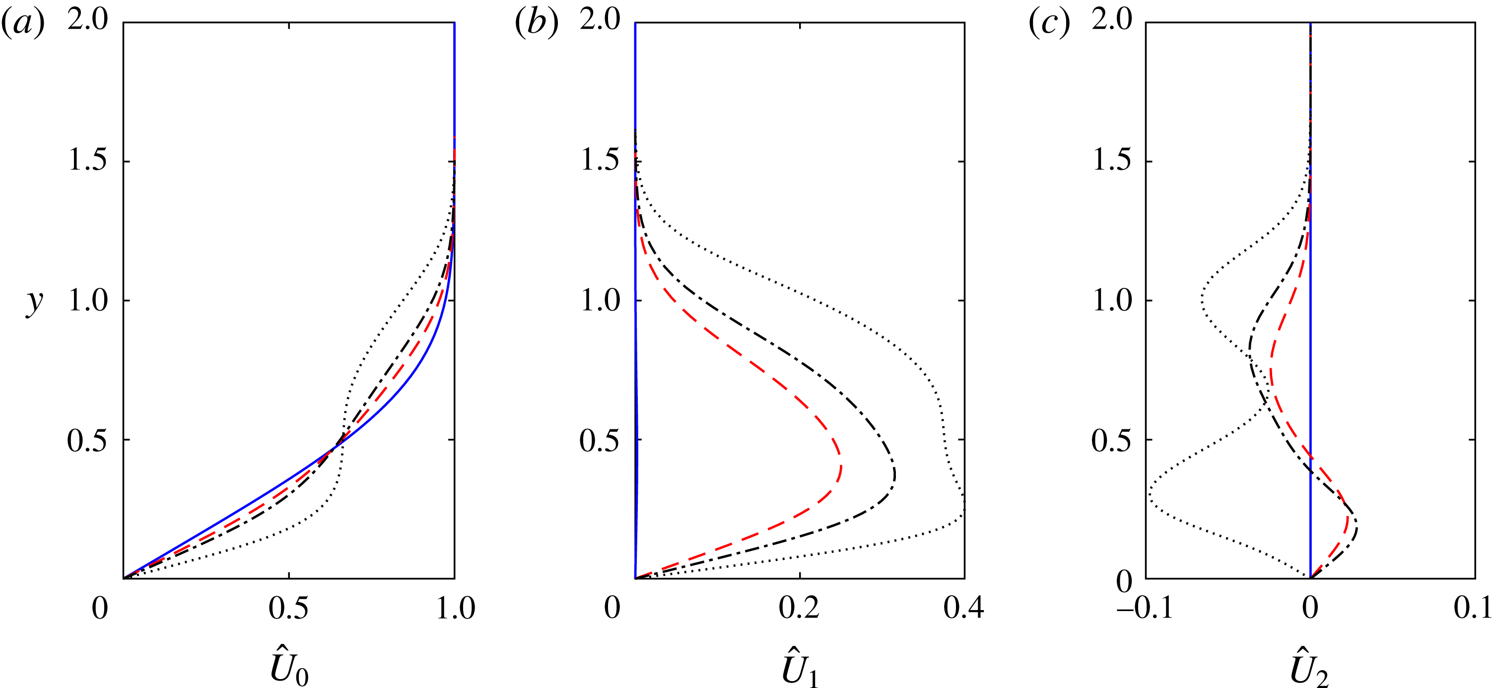
coordinate is used as a parameter. The base flow for the secondary stability analysis is extracted from the DNS at the peak location of the streak and decomposed into a Fourier series. Before proceeding to the stability analysis, let us first examine the spanwise harmonics of the base flow. These are shown in figure 18 for case 3 in table 1, for initial energies of
 $10^{-8}$
,
 $5\times 10^{-5}$
,
 $10^{-4}$
and
 $4\times 10^{-4}$
. As the initial energy increases, the streak widens along the wall-normal coordinate and the mean flow modification becomes more significant. The streak amplitudes, defined as
 $A_{u}=\max |U(y,z)-\hat{U} _{0}(y)|$
, where
 $\hat{U} _{0}$
is the spanwise mean of
 $U$
, are 26 %, 32 % and 50 % for
 $E_{0}=5\times 10^{-5}$
,
 $10^{-4}$
and
 $4\times 10^{-4}$
, respectively. These streak amplitudes are similar to (26 %) and greater than (32 % and 50 %) the critical values for instability obtained by Andersson et al. (Reference Andersson, Brandt, Bottaro and Henningson2001) for a flat plate using an inviscid analysis. Statistical results of streaks in boundary layers subjected to free-stream turbulence by Hack & Zaki (Reference Hack and Zaki2014) showed comparable amplitudes.
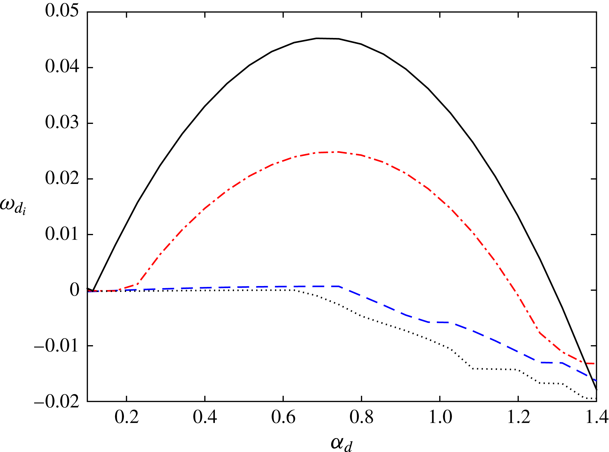
Our next step is performing a secondary stability analysis of the streaks. All four types of instability, namely fundamental varicose, subharmonic varicose, fundamental sinuous and subharmonic sinuous, were calculated for various streamwise wavenumbers. The growth rates of the least stable eigenfunctions for each instability type are presented in figure 19 for case 3 in table 1 and an initial energy of
 $E_{0}=10^{-4}$
. The most unstable disturbance is subharmonic sinuous, similarly to previous findings in flat plate boundary layers (e.g. Andersson et al.
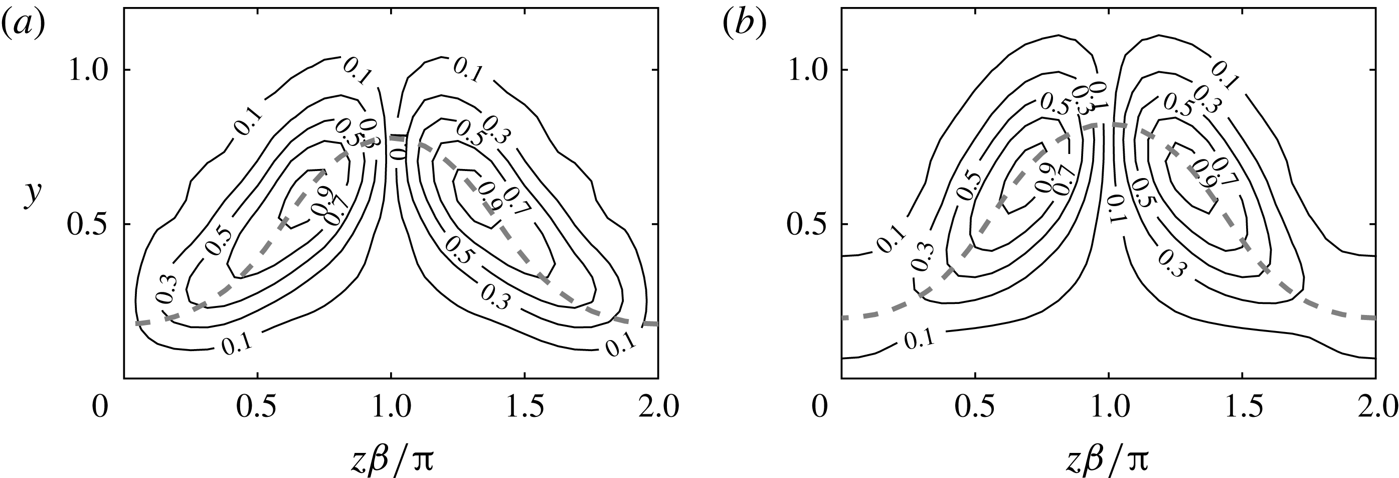
Reference Andersson, Brandt, Bottaro and Henningson2001; Vaughan & Zaki Reference Vaughan and Zaki2011). The fundamental sinuous mode is unstable as well, but reaches a lower maximal growth rate, whereas the varicose disturbances are close to neutrally stable. The magnitude of the streamwise component corresponding to the fundamental and subharmonic sinuous modes is shown in figures 20(a) and 20(b) respectively. It can be seen that both modes have a similar shape, associated with spanwise shear on both sides of the low-speed streak at
 $z\unicode[STIX]{x1D6FD}/\unicode[STIX]{x03C0}=1$
. Both modes also closely follow the critical layer, indicated in the figure by the dashed line. It should be noted that only half the spanwise wavelength of the subharmonic disturbance is plotted since its magnitude has the same periodicity as the base flow.
Growth rate of secondary instabilities for case 3 in table 1 and initial energy of
 $10^{-4}$
. Fundamental varicose (dashed line), fundamental sinuous (dash-dotted line), subharmonic varicose (dotted line) and subharmonic sinuous (solid line).

The streamwise magnitude of the most unstable secondary disturbances for case 3 in table 1 and initial energy of
 $10^{-4}$
. (a) Fundamental sinuous. (b) Subharmonic sinuous. The dashed line marks the critical layer.

The secondary disturbance growth rate consists of production from wall-normal shear, spanwise shear and curvature, and viscous dissipation. To examine the dominance of different components, a volumetric integral of the secondary disturbance kinetic energy equation is performed (e.g. Cossu & Brandt Reference Cossu and Brandt2004). The following equation of the growth rate is obtained:
 $$\begin{eqnarray}\unicode[STIX]{x1D714}_{d_{i}}=\frac{T_{y}}{2E_{d}}+\frac{T_{z}}{2E_{d}}+\frac{T_{\unicode[STIX]{x1D705}}}{2E_{d}}-\frac{D}{2E_{d}},\end{eqnarray}$$
where
 $\unicode[STIX]{x1D714}_{d_{i}}$
is the growth rate,
 $E_{d}$
is the kinetic energy of the secondary disturbance,
 $T_{y}$
,
 $T_{z}$
and
 $T_{\unicode[STIX]{x1D705}}$
are the energy production terms associated with the wall-normal shear, spanwise shear and curvature, respectively, and
 $D$
is the viscous dissipation given by the square norm of the perturbation vorticity
 $(\unicode[STIX]{x1D709}_{d},\unicode[STIX]{x1D702}_{d},\unicode[STIX]{x1D701}_{d})^{\text{T}}$
. The integral expressions are
 $$\begin{eqnarray}E_{d}=\frac{1}{L_{z}}\int _{0}^{L_{z}}\int _{0}^{\infty }\tilde{e}\,\text{d}y\,\text{d}z,\quad \hphantom{\frac{\unicode[STIX]{x2202}U}{\unicode[STIX]{x2202}y};,}D=\frac{1}{L_{z}}\int _{0}^{L_{z}}\int _{0}^{\infty }\tilde{d}\,\text{d}y\,\text{d}z,\hphantom{\frac{\unicode[STIX]{x2202}U}{\unicode[STIX]{x2202}y};,}\end{eqnarray}$$
 $$\begin{eqnarray}T_{y}=\frac{1}{L_{z}}\int _{0}^{L_{z}}\int _{0}^{\infty }\tilde{\unicode[STIX]{x1D70F}}_{uv}\frac{\unicode[STIX]{x2202}U}{\unicode[STIX]{x2202}y}\,\text{d}y\,\text{d}z,\quad T_{z}=\frac{1}{L_{z}}\int _{0}^{L_{z}}\int _{0}^{\infty }\tilde{\unicode[STIX]{x1D70F}}_{uw}\frac{\unicode[STIX]{x2202}U}{\unicode[STIX]{x2202}z}\,\text{d}y\,\text{d}z,\hspace{2.4pt}\end{eqnarray}$$
 $$\begin{eqnarray}T_{\unicode[STIX]{x1D705}}=\frac{1}{L_{z}}\int _{0}^{L_{z}}\int _{0}^{\infty }(-2\unicode[STIX]{x1D705})\tilde{\unicode[STIX]{x1D70F}}_{uv}U\,\text{d}y\,\text{d}z,\qquad \quad\end{eqnarray}$$
where
 $$\begin{eqnarray}\tilde{e}=\tilde{u} _{d}\tilde{u} _{d}^{\ast }+\tilde{v}_{d}\tilde{v}_{d}^{\ast }+\tilde{w}_{d}\tilde{w}_{d}^{\ast },\quad \tilde{d}=2(\tilde{\unicode[STIX]{x1D709}}_{d}\tilde{\unicode[STIX]{x1D709}}_{d}^{\ast }+\tilde{\unicode[STIX]{x1D702}}_{d}\tilde{\unicode[STIX]{x1D702}}_{d}^{\ast }+\tilde{\unicode[STIX]{x1D701}}_{d}\tilde{\unicode[STIX]{x1D701}}_{d}^{\ast })/Re,\end{eqnarray}$$
 $$\begin{eqnarray}\tilde{\unicode[STIX]{x1D70F}}_{uv}=-(\tilde{u} _{d}\tilde{v}_{d}^{\ast }+\tilde{u} _{d}^{\ast }\tilde{v}_{d}),\quad \hphantom{\tilde{w}_{d}}\tilde{\unicode[STIX]{x1D70F}}_{uw}=-(\tilde{u} _{d}\tilde{w}_{d}^{\ast }+\tilde{u} _{d}^{\ast }\tilde{w}_{d}).\hphantom{\tilde{w}_{d}\tilde{w}_{d}^{\ast }/Re_{uw}}\end{eqnarray}$$
The components of the growth rate for the two most unstable sinuous secondary disturbances, shown in figure 20, are presented in table 2, along with their corresponding streamwise wavenumber and phase velocity. For both fundamental and subharmonic disturbances the dominant term is the spanwise production (
 $T_{z}$
). Furthermore, the effect of the curvature on the growth rate of the secondary instability is negligible. The analysis has been repeated for an initial energy of
 $E_{0}=4\times 10^{-4}$
and the growth rates are shown in table 2. Due to the increase in energy, the growth rates of both sinuous instabilities become very close. Most of the change in the growth rate is associated with wall-normal production (
 $T_{y}$
), without any significant contribution of the wall curvature. The negligible contribution of the curvature can be anticipated by comparing the expressions for
 $T_{y}$
and
 $T_{\unicode[STIX]{x1D705}}$
in (5.3a
) and (5.4). Both terms contain
 $\tilde{\unicode[STIX]{x1D70F}}_{uv}$
, which is concentrated in the boundary layer (see the streamwise component in figure 20). The wall-normal production is calculated by an integral weighted with
 $(\unicode[STIX]{x2202}U/\unicode[STIX]{x2202}y)$
. The integrand of the production as a result of the curvature is multiplied by
 $(-2\unicode[STIX]{x1D705}U)$
, which is considerably smaller than
 $(\unicode[STIX]{x2202}U/\unicode[STIX]{x2202}y)$
inside the boundary layer. Therefore, we conclude that the nature of the streak instabilities found here is quite similar to those of the flat boundary layer and the effect of the curvature is mainly on the primary disturbance which generates the streaks.
Growth rate components, streamwise wavenumber and phase velocity for the most unstable sinuous instabilities of case 3 in table 1 for initial energies
 $10^{-4}$
and
 $4\times 10^{-4}$
.

6 DNS of secondary instabilities
In the previous section the dominant secondary instabilities of the streaks above a curved wall were examined using linear analysis. The nonlinear behaviour of the secondary instability of the streaks is studied in the following by means of direct numerical simulation. The primary disturbance, generating the streaks, is imposed at the inflow together with a secondary disturbance. Prior to imposing the secondary disturbance at the inflow we convert the results from the temporal stability analysis to spatial stability results, which enables direct comparison with the spatially evolving DNS. For this purpose, the approximation proposed by Gaster (Reference Gaster1962) is utilized,
 $$\begin{eqnarray}\unicode[STIX]{x1D714}_{sec}\approx \unicode[STIX]{x1D714}_{d_{r}},\quad \unicode[STIX]{x1D6FC}_{sec_{i}}\approx -\frac{\unicode[STIX]{x1D714}_{d_{i}}}{\unicode[STIX]{x2202}\unicode[STIX]{x1D714}_{d_{r}}/\unicode[STIX]{x2202}\unicode[STIX]{x1D6FC}_{d}},\end{eqnarray}$$
where
 $\unicode[STIX]{x1D714}_{sec}$
and
 $-\unicode[STIX]{x1D6FC}_{sec_{i}}$
are respectively the approximate frequency and spatial growth rate of the secondary disturbance and
 $\unicode[STIX]{x2202}\unicode[STIX]{x1D714}_{d_{r}}/\unicode[STIX]{x2202}\unicode[STIX]{x1D6FC}_{d}$
is the real component of the group velocity.
The investigation is based on the subharmonic sinuous mode which becomes unstable first. For the primary disturbance generating the transient growth, the following parameters are used:
 $Re=2100$
,
 $\unicode[STIX]{x1D6FD}=1.85$
and
 $\unicode[STIX]{x1D714}=0$
. Several scenarios, corresponding to different curvatures and initial energies, are investigated, as detailed in table 3. The table shows the frequency of the disturbance injected to the DNS (
 $\unicode[STIX]{x1D714}_{sec}$
) and the approximate spatial growth rate (
 $-\unicode[STIX]{x1D6FC}_{sec_{i}}$
) predicted by the linear analysis. The following numerical parameters are used:
 $(L_{x},L_{y},L_{z})=(200,30,4\unicode[STIX]{x03C0}/\unicode[STIX]{x1D6FD})$
with
 $(N_{x},N_{y},N_{z})=(1024,192,64)$
. The initial energy of the secondary disturbance for all cases is
 $E_{sec}(x=0)=10^{-6}$
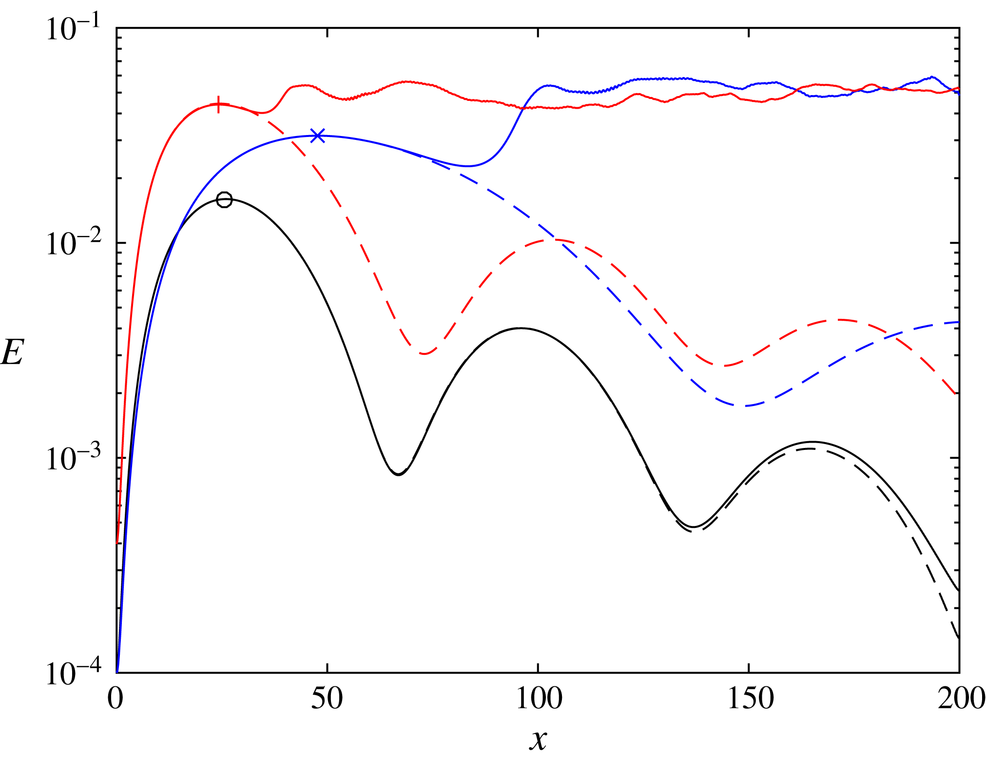
. Case A is based on the secondary disturbance given in row 2 of table 2. When injecting this secondary disturbance into the DNS, no transition to turbulence was observed. The energy for case A is indicated in figure 21 by the solid line marked by a circle. The dashed line represents the same scenario without a secondary disturbance, i.e. only transient growth. As transition does not occur, the solid and dashed curves follow one another closely. To better understand whether an instability is present in this scenario, a spanwise Fourier decomposition of the streamwise velocity is performed. First, the streamwise velocity is decomposed,
 $$\begin{eqnarray}u=\mathop{\sum }_{n=0}^{\infty }u_{n}(t,x,y)\text{e}^{\text{i}\unicode[STIX]{x1D6FD}nz},\end{eqnarray}$$
where
 $n=0,1/2,\ldots$
is the multiplier of the fundamental spanwise wavenumber. Then, the Fourier components are time averaged and integrated along the wall-normal direction,
 $$\begin{eqnarray}a_{n}(x)=\frac{1}{T_{sec}}\int _{0}^{T_{sec}}\int _{0}^{\infty }|u_{n}(t,x,y)|\,\text{d}y\,\text{d}t,\end{eqnarray}$$
where
 $T_{sec}=2\unicode[STIX]{x03C0}/\unicode[STIX]{x1D714}_{sec}$
is the period of the secondary disturbance. The coefficients
 $a_{n}(x)$
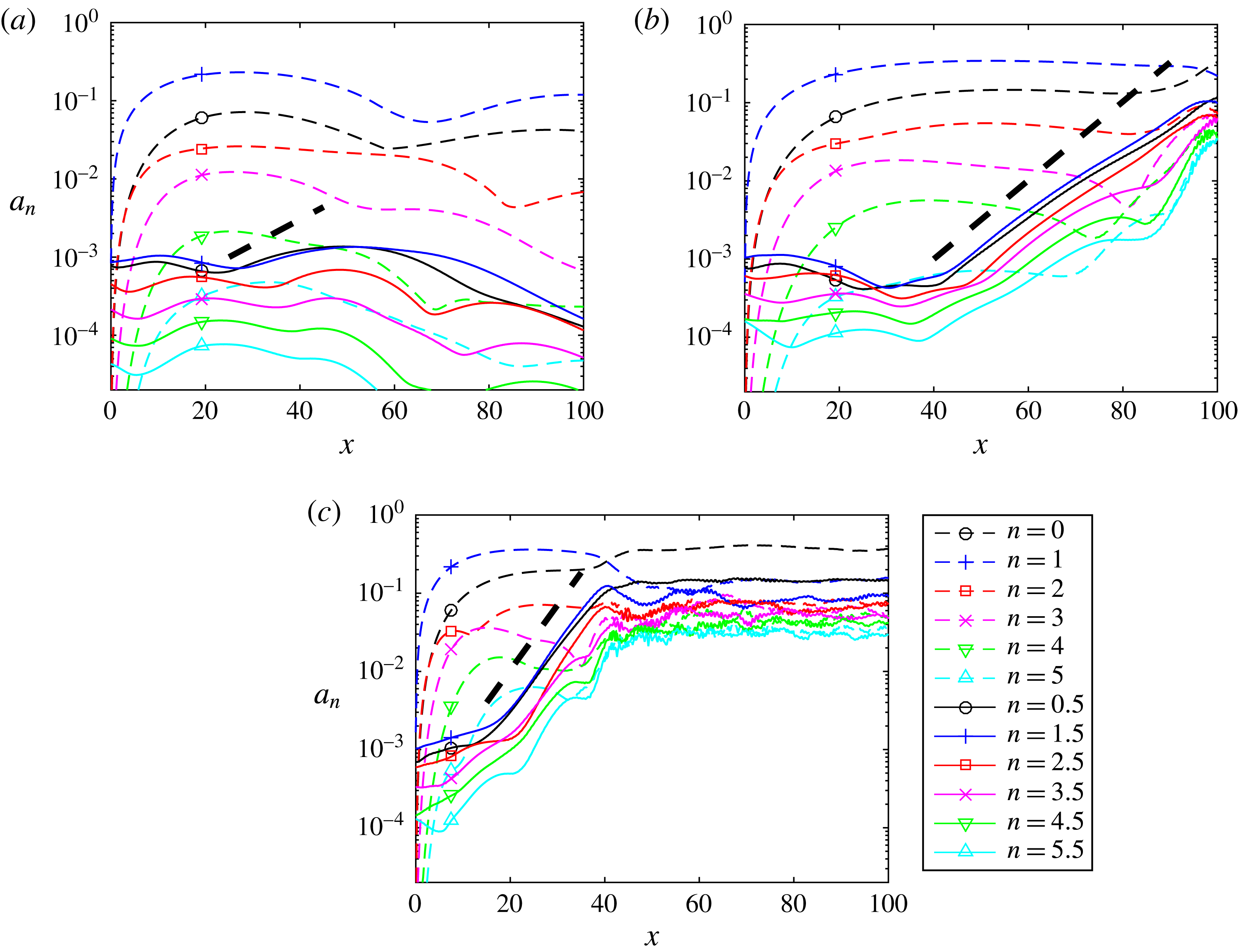
for case A are presented in figure 22(a). The dashed and solid curves correspond to fundamental (
 $0,1,\ldots$
) and subharmonic (
 $1/2,3/2,\ldots$
) spanwise wavenumbers, respectively. The subharmonic wavenumbers do not grow initially. As the streak reaches its maximum (
 $x=26$
), the subharmonic components begin to grow mildly. Nevertheless, the streaks decay before they reach magnitudes sufficient to trigger transition. The predicted growth rate (
 $-\unicode[STIX]{x1D6FC}_{sec_{i}}$
) is indicated by the thick dashed line superimposed on the figure. The actual growth rate is smaller and the approximation may be adequate only in the small vicinity of the streak maximum (
 $x=26$
). A possible explanation for the discrepancy is that the secondary stability assumption on separation of scales, between the rate of change of base flow and secondary disturbance, is not fulfilled here. From case A we conclude that the transition to turbulence is precluded by two factors: (i) the streak is too short to allow transition to turbulence; (ii) the growth rate of the secondary disturbance is not high enough. To examine the above conjectures two additional cases are explored. These are cases B and C in table 3.
Energy growth for cases A (marked by circle), B (marked by cross) and C (marked by plus) in table 3, where subharmonic sinuous disturbances are injected on top of primary disturbances. The dashed lines represent reference simulations without secondary disturbances.

Subharmonic sinuous disturbances used for the DNS. For all cases
 $Re=2100$
,
 $\unicode[STIX]{x1D6FD}=1.85$
and
 $\unicode[STIX]{x1D714}=0$
.

Spanwise Fourier components of the streamwise velocity. The thick dashed line represents the predicted growth rate (
 $-\unicode[STIX]{x1D6FC}_{sec_{i}}$
) from the linear secondary stability analysis. Panels (a–c) correspond to cases A–C in table 3.

In case B, the radius is multiplied by a factor of 4 relative to case A. This results in a twofold elongation of the streaks and a higher streak amplitude, as evident by comparing the dashed lines of cases A (marked by a circle) and B (marked by a cross) in figure 21. Comparing cases A and B in table 3, the growth rate of the secondary disturbance increases by
 ${\sim}60\,\%$
. When injecting the secondary disturbance into the DNS, the flow transitions to turbulence around
 $x\approx 90$
as seen from the solid line marked by a cross in figure 21. The coefficients
 $a_{n}(x)$
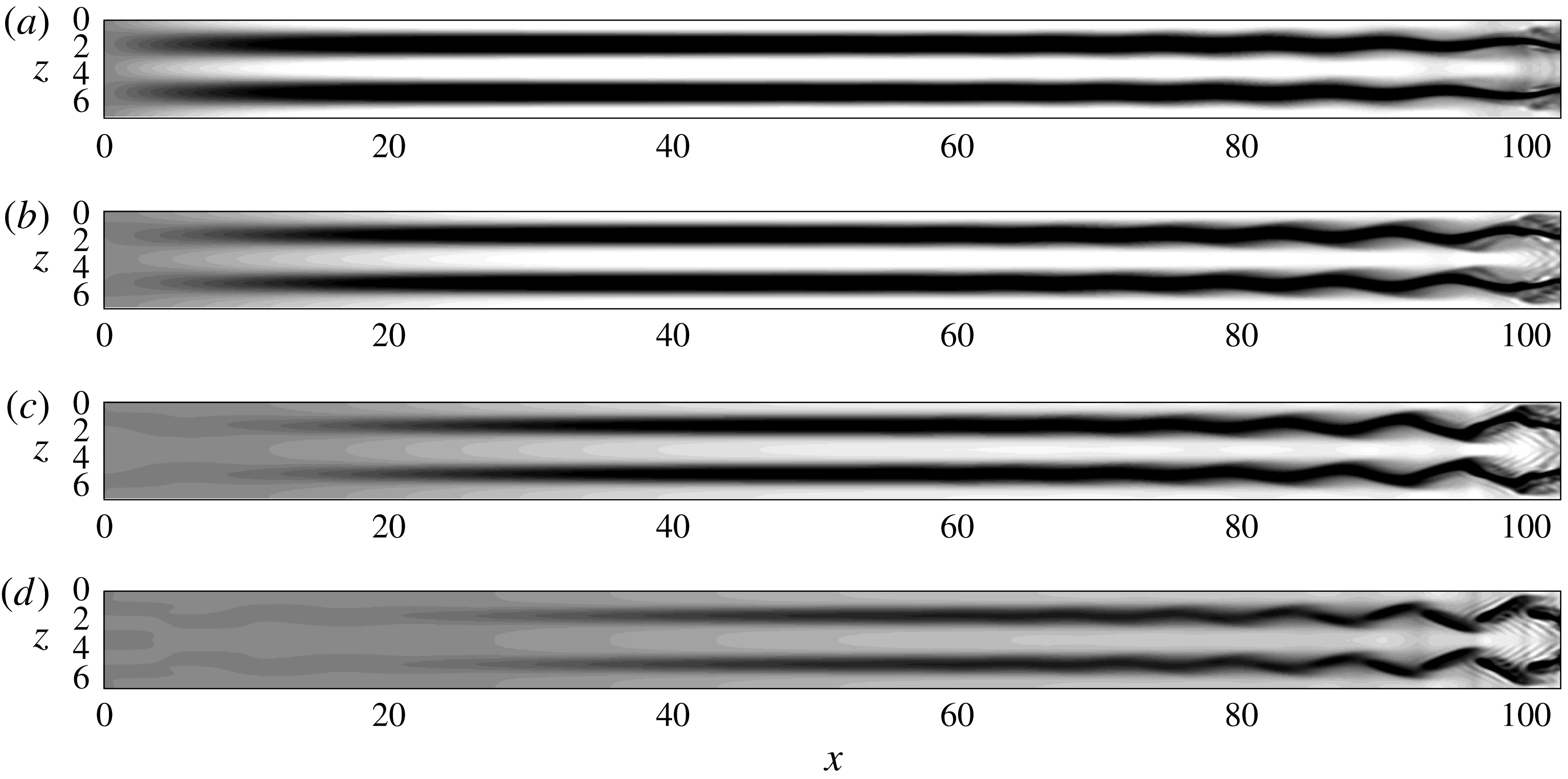
for case B are presented in figure 22(b). The subharmonic wavenumbers (solid curves) do not grow initially; however, once the streak reaches its maximum, a sharp exponential growth is observed, leading to turbulence. The estimated spatial growth rate given in table 3 is superimposed on the figure by the thick dashed line and good agreement is observed with the actual growth rate in the DNS (the slope of the solid lines). Visualization of the transition scenario is presented in figure 23, which shows top views of the streaks for several wall-normal locations. The contours range between
 $-0.2$
(black) and 0.2 (white). Sinuous oscillations of the low-speed streaks are observed, with the largest fluctuations around
 $y=0.75$
(figure 23
b) to
 $y=1$
(figure 23
c). A streamwise wavelength of
 ${\sim}8$
(corresponding to a wavenumber of 0.79) is seen in the figure, which is within 10 % of 0.86, the estimated streamwise wavenumber in table 3.
Top views of streaks for case B in table 3, for several wall-normal locations, visualized by contours of streamwise disturbance velocity in the range
 $-0.2$
(black) to 0.2 (white). Flow from left to right. (a)
 $y=0.5$
. (b)
 $y=0.75$
. (c)
 $y=1$
. (d)
 $y=1.25$
.

In case C, the initial energy is increased by a factor of 4 compared to case A. This results in significantly higher streak amplitude and minor elongation, as observed by comparing the dashed lines of cases A (marked by a circle) and C (marked by a plus) in figure 21. The growth rate of the secondary disturbance increases by a factor of 2.5, as evident by comparing cases A and C in table 3. When including this secondary disturbance in the DNS, the flow transitions to turbulence around
 $x\approx 40$
as seen from the solid line marked by a plus in figure 21. The coefficients
 $a_{n}(x)$
for case C are presented in figure 22(c). As in the previous scenarios, the subharmonic wavenumbers grow exponentially once the streak reaches its maximal amplitude. Excellent agreement is observed between the estimated spatial growth rate, given in table 3 (indicated by the thick dashed line in figure 22
c), and the actual growth rate obtained in the DNS (the slope of the solid lines). A visualization of the transition scenario is presented in figure 24, which shows streaks of
 $\pm 0.1$
streamwise disturbance velocity in red (positive) and blue (negative). A movie spanning over one period of the secondary disturbance is available in supplementary material at https://doi.org/10.1017/jfm.2018.690. Sinuous fluctuations of the low-speed streaks are seen. The breakdown to turbulence occurs rapidly over two streamwise oscillations and the flow becomes fully turbulent downstream.
Streamwise streaks for case C in table 3, visualized by isosurfaces of
 $\pm 0.1$
streamwise disturbance velocity (positive, red; negative, blue). Flow from left to right. An animation is available as part of the supplementary material.

To summarize, in case B transition to turbulence is achieved due to a combination of the longer streak and higher streak amplitude, whereas in case C the very high streak amplitude leads to the same outcome. Therefore, for transition to turbulence to occur on a convex surface, the initial set of streaks should be long enough and reach a sufficiently high amplitude. As the curvature increases the streaks shorten, thus, for higher curvatures, higher streak amplitudes are required.
7 Transient growth at constant Görtler number
The analysis presented so far discusses constant curvature surfaces. For boundary layers evolving on a constant curvature surface the Görtler number increases with
 $x$
due to the increase in the local Reynolds number (see figure 11
b). For the Görtler number to remain constant a reduction of the curvature along the surface is required, which results in a spiral. The mathematical formulation of the spiral is given in appendix B.
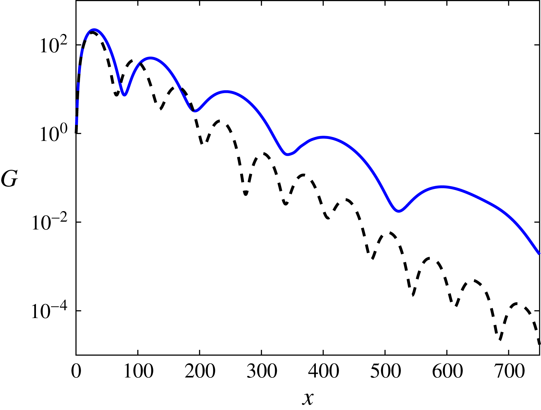
Energy gain obtained from a linear DNS of transient growth over a spiral with constant Görtler number (solid) and constant curvature (dashed). Parameters based on case 3 in table 1.

The transient growth over a spiral is examined for
 $Re=2100$
,
 $\unicode[STIX]{x1D6FD}=1.85$
,
 $\unicode[STIX]{x1D714}=0$
and a curvature of
 $\unicode[STIX]{x1D705}=1/500$
at the inflow location. The linear evolution of the streaks is investigated by setting the amplitude of the streamwise vortices (
 $\max \{\tilde{v}(0,y),\tilde{w}(0,y)\}$
) to
 $10^{-4}$
. Based on the inflow
 $Re$
and
 $\unicode[STIX]{x1D705}$
the shape of the spiral is calculated. Then, the same local optimal disturbance utilized previously for the constant curvature is prescribed at the inflow of the DNS. The energy gain in the flow over the spiral is given by the solid line in figure 25, along with a dashed line representing constant curvature (case 3 in table 1). Due to the decrease in curvature, each set of streaks is longer than its predecessor, as predicted by the relation
 $\unicode[STIX]{x1D706}\sim \unicode[STIX]{x1D705}^{-1/2}$
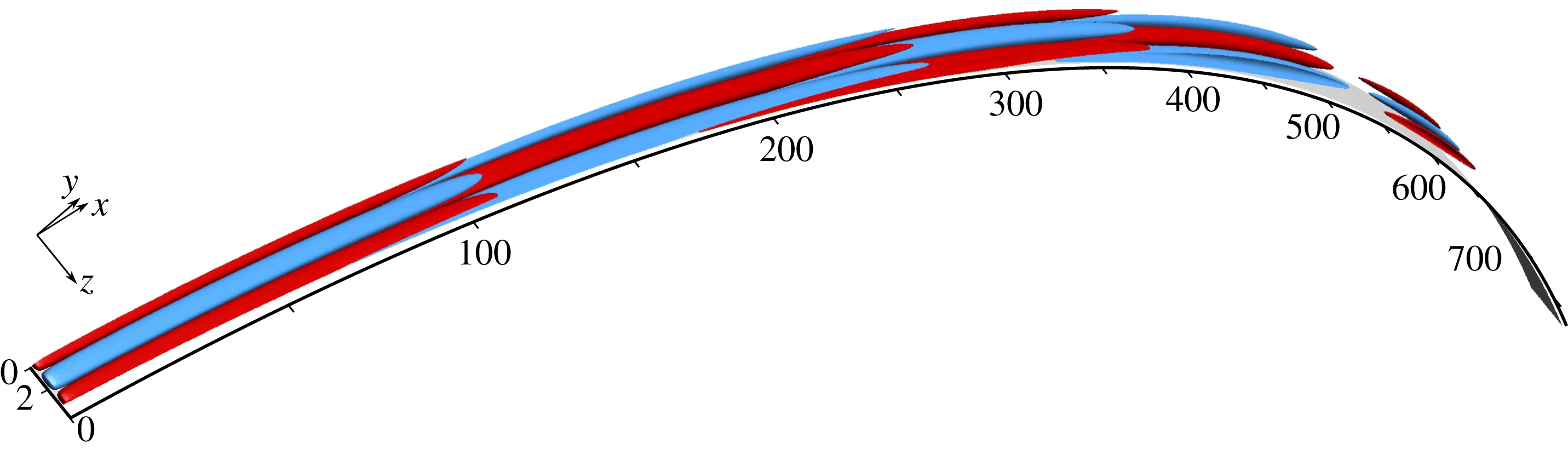
. Another effect is that as a result of the decrease in curvature a higher maximal growth is obtained for the spiral. Moreover, the decay rate of the perturbation is also smaller compared to the constant curvature case. It should be noted that a slight pressure gradient is present for the spiral. This can be explained by inviscid (potential) theory, considering two streamlines, an inner and an outer, following the shape of the spiral, and assuming the velocity is constant along the outer streamline. Since the curvature is decreasing, the pressure gradient normal to the streamline abates as well, which in turn leads to an increase of pressure along the inner streamline. Thus, an adverse pressure gradient is present on the inner streamline which leads to flow deceleration. This effect has been observed in the simulations, but it has a minor effect on the results shown here. The streaks obtained in the DNS are visualized in figure 26 by isosurfaces of 1 % of the maximum streamwise disturbance velocity. Red (blue) represents positive (negative) streaks. As discussed previously for the constant curvature case (figure 15), each set of streaks begins to form below its predecessor, which lifts away from the wall. This is evident in figure 26, especially for the third and fourth sets of streaks.
Streamwise streaks obtained from a linear DNS of transient growth over a spiral with constant Görtler number. Streaks are visualized by isosurfaces of 1 % of the maximum streamwise disturbance velocity (positive, red; negative, blue). Flow from left to right.

8 Summary and concluding remarks
The non-modal instability of boundary layers over convex surfaces is analysed. For steady disturbances, the optimal disturbance corresponds to alternating streaks and streamwise vortices of opposite sign that reinforce one another due to lift-up and centrifugal forces, respectively. The process repeats with a constant streamwise wavelength proportional to
 $\unicode[STIX]{x1D705}^{-1/2}$
. The role of various parameters such as disturbance spanwise wavenumber and frequency, as well as the curvature, is studied using the local stability theory. DNS are used to calculate the exact evolution of the disturbances including non-parallel and nonlinear effects. The simulations confirm the predictions of the local stability theory and the scaling of the streamwise wavelength with
 $\unicode[STIX]{x1D705}^{-1/2}$
. For steady disturbances the resulting streamwise wavelength is longer for smaller spanwise wavenumbers. The optimal spanwise wavenumber increases with the curvature (
 $\widetilde{G\ddot{o} }$
), whereas the optimal growth and the location where it is obtained decrease. For a given curvature the optimal disturbance is found to be for
 $\unicode[STIX]{x1D714}\neq 0$
as a result of the opposing effects of the lift-up and centrifugal mechanisms. The mechanism behind the reduction in growth is analysed and it is found that the pressure redistribution for disturbances with
 $\unicode[STIX]{x1D714}\neq 0$
is more dominant than the production as a result of the curvature.
Secondary stability analysis of the streaks indicates that the curvature has a negligible effect on the secondary disturbances and the instabilities are comparable to their counterparts for a flat plate boundary layer. It has been found that the presence of a secondary instability is not sufficient, on its own, to ensure transition to turbulence. To achieve turbulent flow, the streaks should be long enough or have a sufficiently high amplitude. This suggests that streaks over convex surfaces can be used efficiently to delay transition to turbulence. Very good agreement is observed between the estimated growth rates, obtained from the secondary stability analysis, and the actual growth rates in the DNS. These findings confirm our approach based on temporal secondary stability analyses of a parallel base flow, with
 $x$
used as a parameter, followed by an estimation of the spatial growth rate.
Preliminary investigations of a spiral surface with decreasing curvature to maintain a constant Görtler number show that alternating streaks and streamwise vortices are obtained for a spiral as well. The main difference is that for the spiral each set of streaks is longer than its predecessor.
A natural continuation of this work is analysing the effect of pressure gradient to obtain more practical results as flows over curved surfaces usually involve a pressure gradient.
Acknowledgement
This investigation was funded by the Office of Naval Research (ONR) under grant N00014-17-1-2341.
Supplementary material
A supplementary flow animation is available at https://doi.org/10.1017/jfm.2018.690.
Appendix A. Higher-order analysis
In this appendix the effect of including higher-order terms as a result of the curvature in the local stability analysis is examined. The disturbance equations are
 $$\begin{eqnarray}\displaystyle & \displaystyle \frac{\unicode[STIX]{x2202}u}{\unicode[STIX]{x2202}t}+hU_{B}\frac{\unicode[STIX]{x2202}u}{\unicode[STIX]{x2202}x}+(U_{B}^{\prime }+h\unicode[STIX]{x1D705}U_{B})v+h\frac{\unicode[STIX]{x2202}p}{\unicode[STIX]{x2202}x}=\frac{1}{Re}\unicode[STIX]{x1D6FB}_{h}^{2}u, & \displaystyle\end{eqnarray}$$
 $$\begin{eqnarray}\displaystyle & \displaystyle \frac{\unicode[STIX]{x2202}v}{\unicode[STIX]{x2202}t}-2h\unicode[STIX]{x1D705}U_{B}u+hU_{B}\frac{\unicode[STIX]{x2202}v}{\unicode[STIX]{x2202}x}+\frac{\unicode[STIX]{x2202}p}{\unicode[STIX]{x2202}y}=\frac{1}{Re}\unicode[STIX]{x1D6FB}_{h}^{2}v, & \displaystyle\end{eqnarray}$$
 $$\begin{eqnarray}\displaystyle & \displaystyle \frac{\unicode[STIX]{x2202}w}{\unicode[STIX]{x2202}t}+hU_{B}\frac{\unicode[STIX]{x2202}w}{\unicode[STIX]{x2202}x}+\frac{\unicode[STIX]{x2202}p}{\unicode[STIX]{x2202}z}=\frac{1}{Re}\unicode[STIX]{x1D6FB}_{h}^{2}w, & \displaystyle\end{eqnarray}$$
 $$\begin{eqnarray}\displaystyle & \displaystyle h\frac{\unicode[STIX]{x2202}u}{\unicode[STIX]{x2202}x}+\frac{\unicode[STIX]{x2202}v}{\unicode[STIX]{x2202}y}+h\unicode[STIX]{x1D705}v+\frac{\unicode[STIX]{x2202}w}{\unicode[STIX]{x2202}z}=0, & \displaystyle\end{eqnarray}$$
 $\unicode[STIX]{x1D6FB}_{h}^{2}=h^{2}(\unicode[STIX]{x2202}^{2}/\unicode[STIX]{x2202}x^{2})+(\unicode[STIX]{x2202}^{2}/\unicode[STIX]{x2202}y^{2})+(\unicode[STIX]{x2202}^{2}/\unicode[STIX]{x2202}z^{2})$
and
 $h=1/(1+\unicode[STIX]{x1D705}y)$
. These equations are solved using the normal mode assumption, as described in the main text. A comparison of the spectrum with and without the high-order terms for
 $Re=4200$
,
 $\unicode[STIX]{x1D6FD}=1.85$
,
 $\unicode[STIX]{x1D714}=0$
and
 $\unicode[STIX]{x1D705}=1/500\;(\widetilde{G\ddot{o} }=188)$
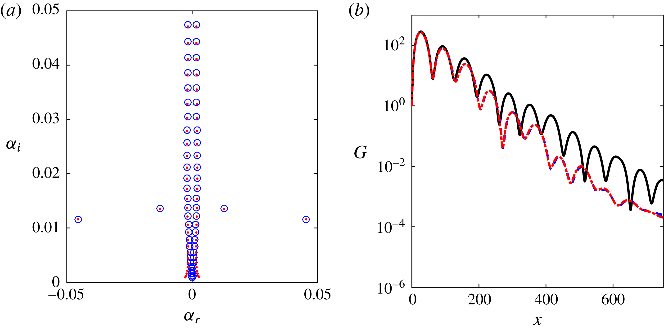
is shown in figure 27(a). The difference is small for the majority of the eigenvalues, with the most significant changes observed close to the origin. A comparison of the energy growth from DNS and theory for case 1 in table 1 is presented in figure 27(b). The DNS is indicated by the solid line, LST with leading-order terms is indicated by the dashed line and LST with higher-order terms is indicated by the dash-dotted line. The LST results remain effectively unchanged.
Comparison between LST results obtained with and without high-order terms as a result of the curvature. (a) Eigenvalues for
 $Re=4200$
,
 $\unicode[STIX]{x1D6FD}=1.85$
,
 $\unicode[STIX]{x1D714}=0$
and
 $\unicode[STIX]{x1D705}=1/500\;(\widetilde{G\ddot{o} }=188)$
. Leading-order (circles) and high-order (dots). (b) Energy gain for case 1 in table 1. Comparison between DNS (solid line), leading-order (dashed line) and high-order (dash-dotted line).

Appendix B. The constant
 $\widetilde{G\ddot{o} }$
spiral

The definition of the spiral derives from the requirement of a constant Görtler number. This prescribes the curvature to satisfy
 $$\begin{eqnarray}\unicode[STIX]{x1D705}(x)=\unicode[STIX]{x1D705}_{0}\left(\frac{Re(x)}{Re_{0}}\right)^{-2}=\unicode[STIX]{x1D705}_{0}\left(1+\frac{x}{x_{0}}\right)^{-1},\end{eqnarray}$$
where
 $\unicode[STIX]{x1D705}_{0}$
is the curvature at the inflow and
 $x_{0}$
is the leading edge location given by
 $Re_{0}$
. By definition, the curvature satisfies the following equation for the slope angle
 $\unicode[STIX]{x1D703}$
:
 $$\begin{eqnarray}\unicode[STIX]{x1D705}(x)=\frac{\text{d}\unicode[STIX]{x1D703}}{\,\text{d}x},\end{eqnarray}$$
which is solved to obtain
 $$\begin{eqnarray}\unicode[STIX]{x1D703}(x)=\unicode[STIX]{x1D705}_{0}x_{0}\ln \left(1+\frac{x}{x_{0}}\right).\end{eqnarray}$$
The spiral shape in Cartesian coordinates (
 $\hat{x},{\hat{y}}$
) is given by
 $$\begin{eqnarray}\hat{x}=\int _{0}^{x}\cos \unicode[STIX]{x1D703}(x^{\prime })\,\text{d}x^{\prime },\quad {\hat{y}}=\int _{0}^{x}\sin \unicode[STIX]{x1D703}(x^{\prime })\,\text{d}x^{\prime },\end{eqnarray}$$
which leads to
 $$\begin{eqnarray}\displaystyle & \displaystyle \hat{x}(\unicode[STIX]{x1D703})=\frac{1}{\unicode[STIX]{x1D705}_{0}}\left(1+\frac{1}{(\unicode[STIX]{x1D705}_{0}x_{0})^{2}}\right)^{-1}\left[\exp \left(\frac{\unicode[STIX]{x1D703}}{\unicode[STIX]{x1D705}_{0}x_{0}}\right)\left(\frac{\cos \unicode[STIX]{x1D703}}{\unicode[STIX]{x1D705}_{0}x_{0}}+\sin \unicode[STIX]{x1D703}\right)-\frac{1}{\unicode[STIX]{x1D705}_{0}x_{0}}\right], & \displaystyle\end{eqnarray}$$
 $$\begin{eqnarray}\displaystyle & \displaystyle {\hat{y}}(\unicode[STIX]{x1D703})=\frac{1}{\unicode[STIX]{x1D705}_{0}}\left(1+\frac{1}{(\unicode[STIX]{x1D705}_{0}x_{0})^{2}}\right)^{-1}\left[\exp \left(\frac{\unicode[STIX]{x1D703}}{\unicode[STIX]{x1D705}_{0}x_{0}}\right)\left(\cos \unicode[STIX]{x1D703}-\frac{\sin \unicode[STIX]{x1D703}}{\unicode[STIX]{x1D705}_{0}x_{0}}\right)-1\right]. & \displaystyle\end{eqnarray}$$