II. Overview

Wine was first produced on the Southern tip of Africa less than a decade after the first permanent settlement by the Dutch in 1652. The purpose of the settlement was to provide a rest and victualling station for ships plying the trade between Europe and the Indies, so there was much experimentation with different types of food and beverages, including wine. This experiment was successful, and viticulture soon became a thriving industry, strengthened by the arrival of the French Huguenots (Fourie and Von Fintel, Reference Fourie and von Fintel2014).

A visual inspection of production trends from these early beginnings shows five “long cycles” in the South African industry (Figure 1), including the first phase of establishment during the 17th century and the subsequent consolidation that took place until 1740. During this period, total production broke the level of 1 million liters (1734) and then fluctuated from a minimum of 400 kl in 1719 to a maximum of 1,100 kl in 1734, but on average remained at around 700 kl. Recorded exports were negligible during this period.

Figure 1

Wine Production in South Africa, 1700–2015 (Kilolitres)

Note: From 1910 measured on the right-hand scale.Source: Anderson and Pinilla (2017).

The second cycle ranged from 1741 to around 1820, a period of relatively rapid growth in production. During these eight decades production increased from 1,000 kl to 9,000 kl, with the average in the last 20 years of this period of around 7,000 kl. There is a definite acceleration in the last half of the period (1780–1820), during which the British fought in wars with France. Exports of wine from the Cape increased from an average of approximately 500 leaguers per year to more than 3,000 leaguers per year until the Cape officially became a colony in 1815, when the tariffs that Cape farmers paid into the UK market declined considerably, with a concomitant increase in exports.

The third cycle encompasses most of the 19th century. During this period, average production increased from around 10,000 kl–15,000 kl to the 1880s, and then increased to over 35,000 kl, only to decline to around 25,000 kl, where it remained until the formation of the Union of South Africa in 1910. After the UK tariff reduction in 1815 the exports of fortified wines soared even more, and continued to do so until 1827–1829, after the 1825 UK tariff revision but before the 1830–1831 reductions in the preference afforded the Cape. Total exports then declined until 1852–1853 and recovered until 1859.

The fourth cycle includes the expansion of the industry throughout the 20th century. During this period, the irrigated areas of the Olifants River (1950s) and then the Orange River (1970s) began to produce. There was also an expansion in production of Estate wines (i.e., where wine was made on the farm where the grapes were grown) with the advent of the Wine Routes concept.

The fifth and final cycle that is easily recognizable is the period after the democratic elections of 1994, accompanied by the demise of apartheid and the international boycotts and sanctions that went with it. The average total output remained level during the first decade, but since then production has increased by around one-third on a total vineyard that was reduced by 1–2% (from 101,000 to 99,000 hectares). An acceleration after 2010 marked the end of the red wine boom, and saw total industry output revert from 30% red in 2004 to 38% in 2011, and then decreased to 34% in 2014. It is also now evident that this final cycle has ended, with the planted area of vines decreasing beyond 95,750 ha in 2016.

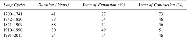
However, Table 1 highlights the danger of a simple interpretation of these longer-term trends. These data show that wine production decreased in 73% of the years that make up the period (30 of the 41 years) and increased in only 11 years.

Table 1

Proportion of Expansionary Versus Contractionary Periods, Wine Production

Source: Calculated from Anderson and Pinilla (Reference Anderson and Pinilla2017).

III. A New Series of Wine Production

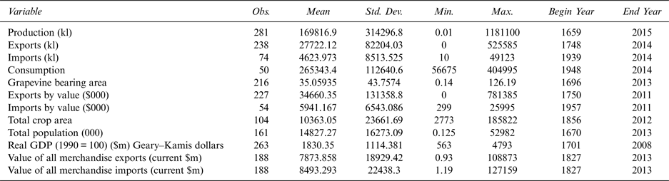
Although several series of South African wine production exist, the purpose was to collate these into one series covering the full period from 1655 to 2016. Information was collected on total production (in kilolitres), exports (kilolitres), imports (kilolitres), total consumption, grapevine bearing area, exports by value, imports by value, total agricultural crop area, total population, real GDP (in 1990 Geary–Khamis dollars), value of all merchandise exports (in current $m) and value of all merchandise imports (also in current $m). Of course, not all series extended until the 17th century. Table 2 provides a descriptive summary of the 12 new measures.

Table 2

Summary Statistics of Twelve New Variables

Source: Anderson and Pinilla (Reference Anderson and Pinilla2017).

Accurate records of Cape wine statistics only begin with the turn of the 18th century. Van Duin and Ross (Reference Van Duin and Ross1987) compiled several series related to Cape wine production, the most important of which is the series on the amount of wine produced. This source forms the basis of our 18th and early 19th-century estimates. Their series on wine production derives from the opgaafrolle, the annual tax returns for the settler population in the Colony. Tax returns are often an unreliable source, as farmers tend to underreport their production to evade taxes. Yet Van Duin and Ross (Reference Van Duin and Ross1987) argue that this is unlikely to be the case for wine production, especially after the 1740s. After 1743, in contrast to other crops, wine was taxed at entry into Cape Town, instead of on the farm. This was possible because there was only one road into Cape Town, and all farmers were legally bound to sell all the marketable wine to the Company. The reported quantity of wine produced should therefore be a close reflection of the actual quantity produced (it is certainly likely that some wine and brandy was consumed at home, smuggled, or illegally traded with the Khoesan, but the size of this illegal activity is difficult to determine, and unlikely to vary significantly over time.)

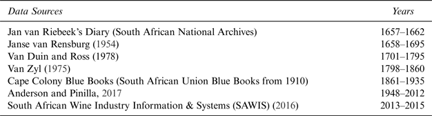
Table 3 gives a summary of the data sources and the years that are used in the compilation of the complete series. A full discussion on the exercise of compilation, sources, and conversions can be found in Van der Merwe and Keywood (Reference Van der Merwe and Keywood2015). Table 4 provides a breakdown of the conversion formula used to convert the different units of wine into the standard measure of kilolitres.

Table 3

Data Sources for Series on Wine Production

Table 4

Conversion Table

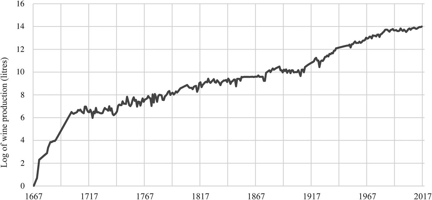
Figure 2 provides an overview of the total wine production. The scale of wine production in the 20th century, and notably between 1950 and 1980, overshadows any significant change during the 18th and 19th centuries. For that reason, the series is drawn on a logarithmic scale.

Figure 2

New Series of Wine Production 1667–2015 in Logarithmic Scale (In Kilolitres)

Source: Anderson and Pinilla (2017).

Figure 2 shows the rapid increase in wine production during the late 18th century as the settler economy expands to meet the need for ships passing through the Cape. Growth seems to slow down for most of the 18th century, and picks up again after the unification and industrial takeoff.

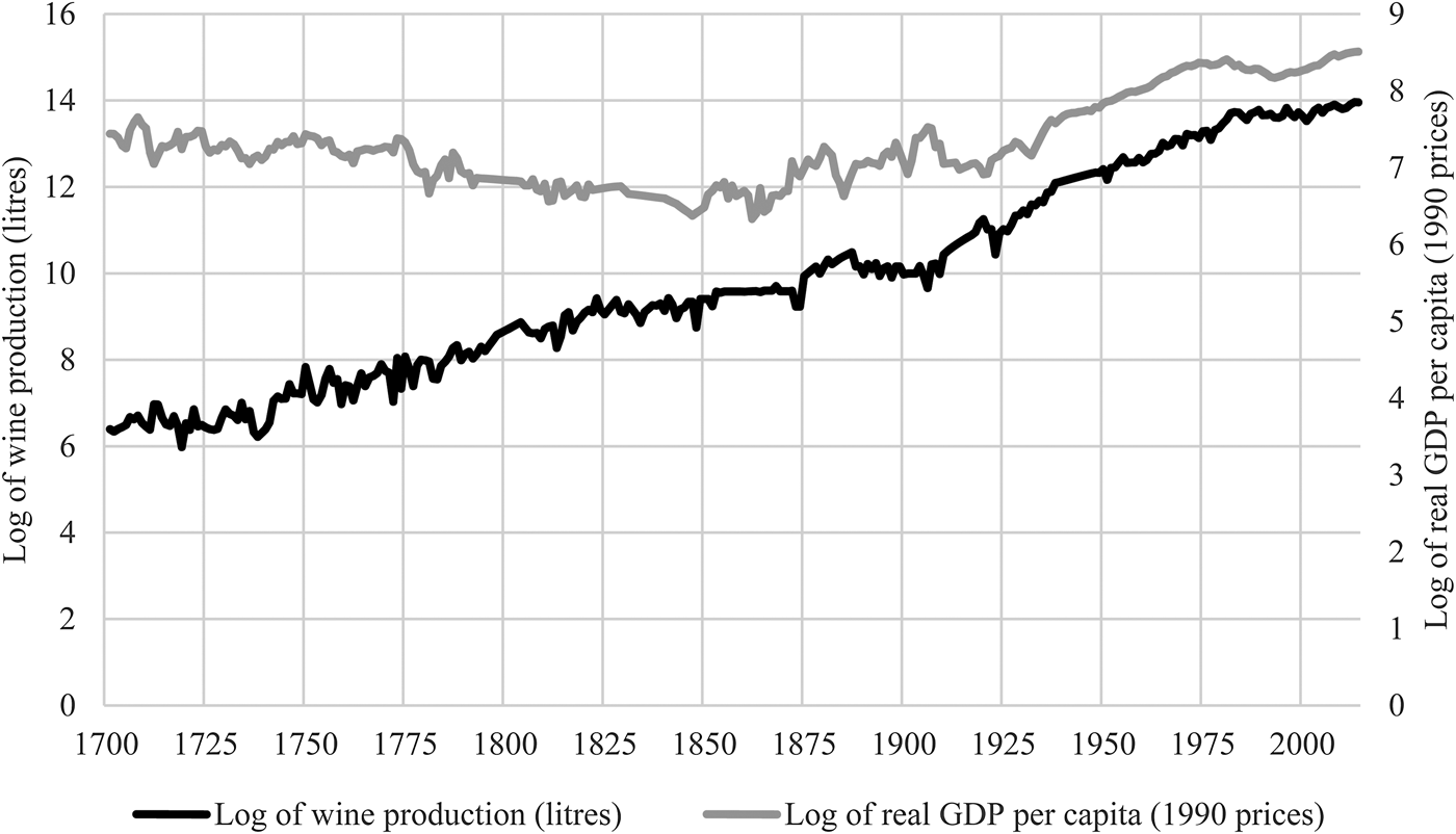
One way to investigate these trends is to juxtapose wine production and GDP per capita (Figure 3). GDP per capita data—in 1990 Geary–Khamis dollars—is obtained from Fourie and Van Zanden (Reference Fourie and Van Zanden2013). The graph suggests a negative correlation between the two series until the 1860s, when the discovery of minerals in the interior of the country drives the economy forward. This is somewhat surprising, given the importance of the historiography that has attributed to the wine industry as a significant driver of Cape prosperity. We do not dispute this positive and possibly causal correlation. We attribute the visible negative correlation instead to the decrease in the per capita GDP series, which is the result of a rapidly expanding frontier economy practicing more expansive, pastoral farming. The denominator (population size) thus increased more rapidly than the numerator (production).

Figure 3

Volume of Wine Production and Real GDP Per Capita, South Africa, 1700 to 2015 (In Logarithms)

Source: Anderson and Pinilla (2017).

IV. Methodology

Empirical analysis is a two-step methodology. First, we use a time-series smoothing technique to extract medium-term cycles. Second, we use a non-parametric method to identify the turning points in the medium-term cycles, in order to arrive at a chronology of medium-term upswings and downswings in wine production.

B. Turning Point Identification

Non-parametric methods for turning point identification rely on the application of calculus rules to the data. These rules have a long history, dating back to the original work of Burns and Mitchell (Reference Burns and Mitchell1946), and were formalized for the first time by Bry and Boschan (Reference Bry and Boschan1971).

All plausible peaks x _t in an annual wine production time-series {x} must satisfy the following calculus rule:

$$\lcub {\lpar {x_{t - k}, \ldots, x_{t - 1}} \rpar \lt{x_t} \gt \lpar {x_{t + 1}, \ldots, x_{t + k}} \rpar } \rcub . $$

Similarly, plausible troughs satisfy:

$$\{ \lpar {x_{t - k}, \ldots, x_{t - 1}} \rpar \gt x_t \lt \lpar {x_{t + 1}, \ldots, x_{t + k}} \rpar \} .$$

This calculus rule sees turning points as local maxima or minima in x. The width of the window k defines the extent to which information is local: it determines the number of data points preceding and following a potential turning point, over which this turning point can be considered a local maximum or minimum. We used k = 2, although the data constraints sometimes required calling a peak or trough based on k = 1.

After potential turning points have been identified, a set of censoring rules are applied to ensure that the turning points alternate (i.e., that peaks follow troughs and vice versa), and that the length of an upward phase (trough-to-peak), a downward phase (peak-to-trough), and a complete cycle (peak-to-peak or trough-to-trough) meet the minimum criteria. In particular, censorship rules specify a minimum duration of two years for a phase and five years for a complete cycle, therefore, they are used to reduce the set of plausible peaks and troughs to the final set.

It is important to note that the calculus rule, as applied previously, identifies so-called classical cycles: in identifying turning points, it requires wine production to contract (or expand) rather than growth in wine production merely to decelerate or accelerate.

Based on the turning points, the duration, amplitude, and steepness of each expansion and contraction can be calculated. The duration is calculated by counting the number of periods in which wine production is expanding or contracting. The expansion (contraction) amplitude is calculated by subtracting the peak (trough) wine production from the preceding trough (peak) wine production. The steepness is calculated by dividing amplitude by the duration, providing a sense of average growth during an expansion or contraction.

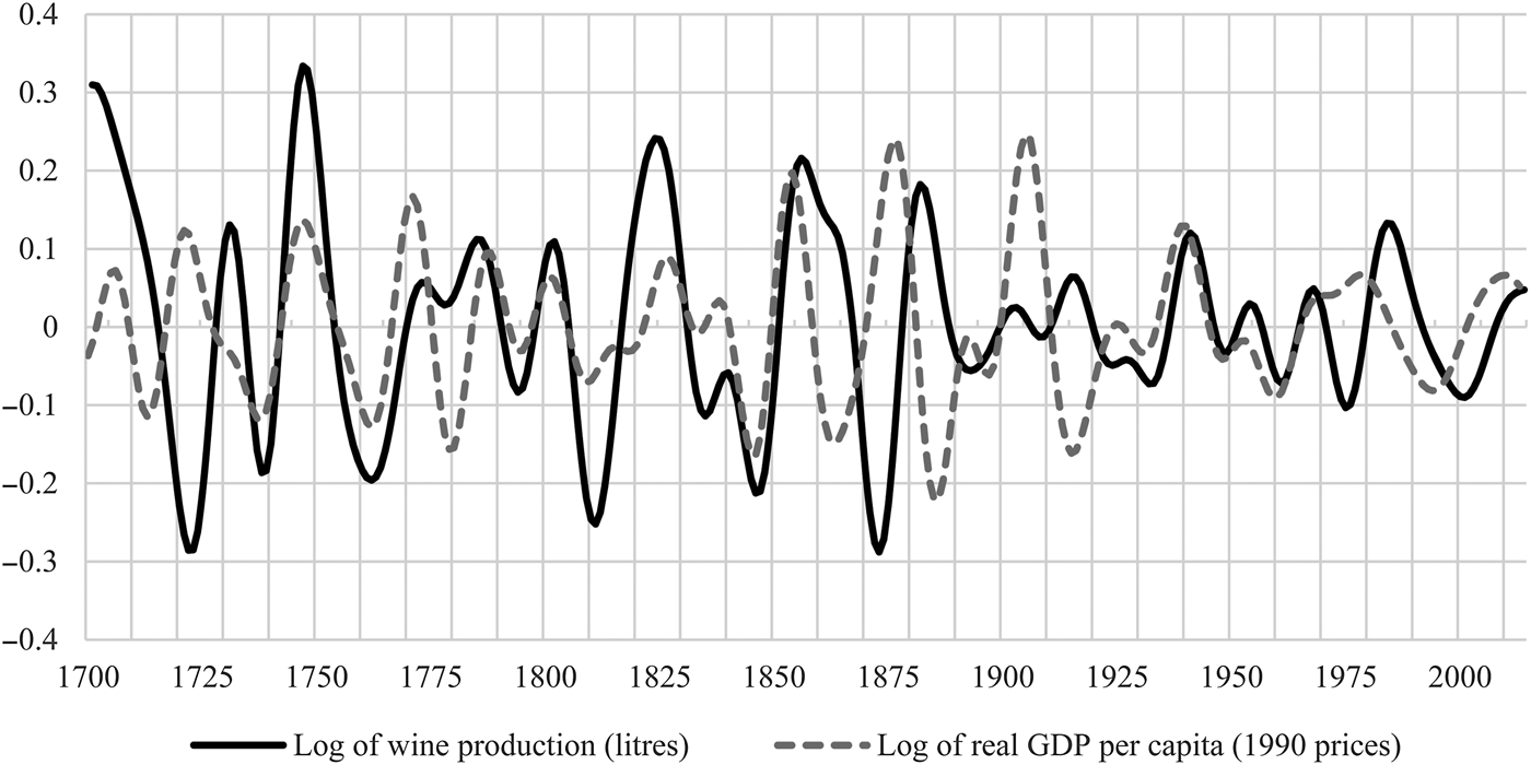
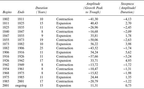
Although the turning point method identifies a large number of expansions and contractions during the 18th century, the phases are shortened from the 19th century onwards (Figure 4). Further, the expansions (contractions) were on average 8.8 (11) years in the 1700s, 10 (14.6) years in the 1800s, and 10.6 (10.4) years in the 1900s. Table 5 shows the most important of these expansionary and contractionary periods.

Figure 4

Medium-Term Cycles in Wine Production and GDP Per Capita in Their Expansion and Contraction Phases, South Africa, 1701 to 2015

Source: Anderson and Pinilla (2017).

Table 5

Properties of the Strongest Expansions and Contractions in Wine Production after 1800

Source: Anderson and Pinilla (Reference Anderson and Pinilla2017).

V. Matching the Analysis and the Story

This analysis shows the transformative periods for South African wine production after 1800:

1. 1. From the late 18th century to 1825, that is, during the Napoleonic wars and their aftermath;

2. 2. In the period following the outbreak of phylloxera (1882–1906);

3. 3. The 20th century, which saw two long periods of relatively slow growth in output and one long period of relatively slow contraction;

4. 4. The contraction that took place in the first phase of the post-apartheid era; and

5. 5. The long expansion of the early 21st Century.

During the first of these periods (from the time of the American War of Independence until the end of the Napoleonic era), Britain either levied high tariffs on French wine imports or completely embargoed them during hostilities (Nye, Reference Nye2007). They also granted a tariff preference to Spain and Portugal, so that the latter had been paying lower tariffs than French exporters from the early 1700s (Nye, Reference Nye2007) and then to Madeira and South Africa, which paid a tariff that was equivalent to only one-third of what the Iberian countries paid (Keegan, Reference Keegan1996).

This boom period for South African wine producers ended with the abolition of imperial preference in 1825, after which the industry contracted almost continuously until 1847. After a brief expansion, the longest contraction followed, coinciding with the repeal of the Corn Laws in Britain in 1846 (Nye, Reference Nye2007) and the Cobden-Chevalier free trade agreement of 1860 with France, which gave French wines duty free access to the British market for the first time in many years. Note that during this period the expansions were generally steeper than the contractions.

The second set of medium-term cycles began in the period around the discovery of diamonds in 1866. The new markets that were created by this and the subsequent discovery of gold represented a potential bonanza for the wine industry, which expanded in the decade until 1882, but then it was brought to a premature end by the global outbreak of phylloxera. Also noteworthy is the discovery of gold in the Witwatersrand in 1886, and the subsequent economic boom (Johannesburg's population was one-third larger than that of Cape Town by 1896) (Van Onselen, Reference Van Onselen1982; Worden, Van Hyningen, and Beckford-Smith, Reference Worden, Van Hyningen and Beckford-Smith1998) had little effect on wine production. This is likely due to the protective tariff levied by the Transvaal Republic on imports of wine from the Cape, together with the Republic's trade treaty with Portugal (Botha, Reference Botha1973).

The third of these sets of medium-term cycles covers the 20th century. The most important events during this time include the long post-Great Depression expansion in the South African economy, which was accompanied by as long an expansion in agricultural production (see also Kirsten, Edwards, and Vink, Reference Kirsten, Edwards, Vink, Anderson and Masters2009; Liebenberg, Reference Liebenberg2012) and in wine production specifically. In the case of wine, the most important intervention was the establishment in 1918 of the Ko-operatieve Wijnbouwersvereeniging van Zuid-Afrika Beperkt (KWV, or Cooperative Wine Farmers’ Association of South Africa, Limited), and then the granting of statutory powers to it in 1930 (Vink, Williams, and Kirsten, Reference Vink, Williams, Kirsten and Anderson2004). However, the post-WWII years saw more declines in production than increases, despite a range of support measures from the state, which included:

• • Government loans to finance the creation of the first co-operative cellars, the precursors of today's producer cellars, which form the backbone of the industry—there were 69 cooperatives by 1975, of which only seven were established before WWII;

• • The expansion in demand for urban labor during the war and the restriction of African migration to the Western Cape until 1976, which created a shortage of farm labor. One consequence was the expansion in the use of prison labor and the establishment of “farm prisons” (Marcus, Reference Marcus1989).

• • In 1963, the sale of alcohol to Africans was legalized and grocers were licensed to sell natural wine (but not beer). There was also further pressure from the industry to stop the dop system of providing wine rations to farm workers in lieu of cash wages, a practice that had been banned in 1809, but was still widely practiced (see also Williams, Reference Williams, Harriss-White and Heyer2009);

• • The further expansion of grape growing in the irrigated areas of Olifants and Orange River, where new distilleries were opened in 1977 and 1978, resulted in the expansion of output far ahead of consumption;

• • In 1979, the Cabinet approved a restructuring of the liquor industry. South African Breweries (later SABMiller and now part of AB Inbev) obtained almost the monopoly of beer sales in South Africa, while Kaapwyn, in which Rembrandt, KWV, and SAB each owned 30% of the shares, was established. Subsequently (in 2001) it resulted in the consolidation of the two largest wine producer wholesalers (Stellenbosch Farmers Winery and Distillers Corporation) into Distell, a firm still controlled by a joint holding company between KWV and Rembrandt, and which has more than 30% share of the domestic wine market;

• • The imposition of boycotts and sanctions against apartheid in South Africa, especially during the 1980s, which reduced exports of South African wines to less than 1% of total production.

The first sustained increase in production during this post-war era occurred after 1975, but the industry had turned the corner in the previous decade. As mentioned earlier, an expansion in wine production may not necessarily be good for producers or the industry in general. Due to the role played by the KWV, in South Africa it usually meant an expansion in the production of low quality wine, reflected in the increasing surpluses declared by the KWV. However, in the late 1960s, a group of farmers in Stellenbosch pioneered a revolution in quality in the industry, and began the process of building wine tourism into the regular offer of their estates (Vink, Williams, and Kirsten, Reference Vink, Williams, Kirsten and Anderson2004).

The fourth of the medium-term cycles consists of a 17-year contraction in post-1985 production (Table 5), which was, in fact, one of the most prosperous periods in the South African industry (at least from around 1987 or 1988). The explanation lies in the rapid replacement of high-yielding varietals such as Chenin Blanc (whose area contracted from one-third of the total in 1985 to less than 20% in 2001), leading to a decline in total wine production from 1 billion litres in 1995 to 750 million litres in 2001. This improvement in the average quality of the South African harvest was accompanied by a rapid expansion in exports as well, although domestic consumption did not increase (Vink et al., Reference Vink, Boshoff, Williams, Fourie, McLean, Anderson and Pinilla2018).

Finally, Table 5 shows the long and continuing expansion after 2001, when producers learned how to increase yields from the relatively low-yielding “noble” varietals, largely by using new clones and new techniques of vineyard management (Vink et al., Reference Vink, Deloire, Bonnardot and Ewert2012). Whether this expansion has now ended remains an open question: visual inspection of the trends clearly shows that the total harvest is beginning to decline, but this may well be the result of idiosyncratic events such as the climate.

The analysis up to this point has focussed on a description of the main production trends that have characterised the industry, but the analysis implies that there is little correlation between GDP and wine cycles. Therefore, the analysis now focuses on the role that exports have played in the expansion of the industry throughout its long history.

VI. What Leads Wine Production?

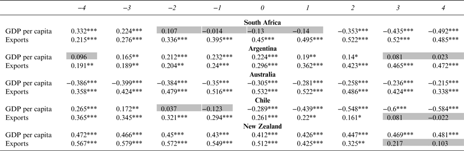
Table 6 shows the Pearson correlation coefficients for the cycles of deviation in wine production with cycles in real GDP per capita and cycles in export volumes, respectively, for the five wine producers of the New World of the Southern Hemisphere. The top row indicates whether the column corresponds to a lag (“–”) or a lead (“+”) of the corresponding variable in the production of wine, and indicates the number of periods separating the observations (e.g., “–3” indicates that the variables in each row have been lagged for three years in relation to the production of wine).

Table 6

The Correlations between Wine Production and GDP Per Capita, and Wine Production and Exports

Note: Statistical significance at the 1 and 5% levels, respectively, is indicated as *** and **.

Source: Anderson and Pinilla, Reference Anderson and Pinilla2017.

The results for South Africa show that the fourth and third lags of GDP per capita are positively related with current-period wine production and are statistically significant at the 1% level. However, the contemporaneous correlation and the correlations in shorter lags are small and statistically insignificant. The coefficients are also negative for the contemporaneous period and the first lag, and are negative and statistically significant (except for the first lead period) at the 1% level for leads of real GDP per capita. These results suggest that South African wine producers react slowly to changes in GDP per capita, and that medium-term cycles in wine production are not strongly related to cycles of domestic wealth. Argentina, Chile, and New Zealand show dynamics that are somewhat similar to those of South Africa in that lags of real GDP per capita are associated with positive coefficients, but they also differ in several important aspects. Chile is most similar to South Africa, with positive and significant fourth- and third-lag correlation coefficients, and with negative and statistically significant coefficients for the contemporaneous relationship and for leads of real GDP per capita. In contrast, wine production and real GDP per capita are associated with positive and significant contemporaneous correlations in New Zealand and Argentina. These countries differ even more from South Africa (and each other) in that the leads of real GDP per capita are positive, but mostly insignificant for Argentina, and are positive and significant for New Zealand. Finally, Australia differs more from these other series; here it appears that medium-term cycles in wine production are countercyclical with medium-term cycles in real GDP per capita. In summary, there are many idiosyncratic features in the relationship between medium-term cycles in wine production and GDP per capita for these countries, and, except for evidence from New Zealand, the cycles in wine production do not appear to be strongly related to the medium cycles in real GDP per capita.

In contrast to the varied results found to characterize the correlation between medium-term cycles in GDP per capita and wine production, the correlation of medium-term cycles in export volumes and wine production are unambiguously positive across all five countries. In South Africa, the volume of exports shows a large degree of statistically significant correlation with wine production. The large, positive, and statistically significant correlations for leads and contemporaneous values of export volume indicate that increases in wine production seem to occur in response to prolonged upswings in the volume of wine exports. The relative magnitude of the coefficients for lags and leads of export volumes provides further evidence that export volumes are an important driver of wine production. Positive coefficients for lags of cycles in export volumes suggest that there is some momentum in production following cycles in exports, while the relatively larger positive correlations for contemporaneous values and leads of export volumes support the notion that when exports increase (decline) over the medium term, wine production follows suit in a sustained manner. Cumulatively, this evidence can be interpreted as supporting the argument that South African wine production has traditionally been driven by exports rather than changes in the GDP per capita that drive domestic consumption.

As for the other four countries, all show positive correlations with wine production for both lags and leads of export volumes. In Argentina and Australia, leads of export volumes show the strongest correlation with contemporaneous production, suggesting that, like South Africa, high current production volumes are associated with prolonged buoyancy in wine export volumes. By contrast, Chile and New Zealand are characterized by slightly different dynamics to those that we see in South Africa. In these countries, the largest correlations are with lags of export volumes, suggesting here that there is a high degree of momentum in domestic production following buoyant export volumes. However, it should also be noted that for Chile the correlation coefficient for the first lead in wine production is the only lead that is statistically significant at the 5% level. Similarly, leads of export volumes are significant up to the second lead for New Zealand. While the general direction of future cycles in exports do not appear to be as strongly related to contemporaneous production in Chile and New Zealand as in South Africa, Argentina, and Australia, the evidence still suggests that prolonged cycles of export volumes have an impact on contemporaneous production. Thus, in summary, while the dynamics of the relationship between cycles in export volumes and in wine production in South Africa, Chile, and New Zealand appear to differ somewhat from those in Argentina and Australia, evidence from all of these countries suggests that cycles in export volumes are an important driver of wine production, more so even than domestic consumption.

VII. Discussion and Conclusion

Wine production in South Africa has a long history that began shortly after the establishment of the first Dutch settlement in 1652. The subsequent arrival of the French Huguenots gave rise to new advances. There are several series on wine production in South Africa. These series cover several periods and make use of different sources. This article contributes to the well-known data sources by providing a single series for wine production in South Africa dating back to 1666.

The new series of wine production together with real GDP per capita from Fourie and Van Zanden (Reference Fourie and Van Zanden2013) enables a cyclical analysis covering more than 300 years. In this regard, the band-pass filter of the business cycle literature is used to separate short-run cycles from long-run trends. The results indicate that cycles in wine production are somewhat unrelated to similar cycles in real GDP per capita. Wine producers, therefore, react slowly to medium-term changes in real GDP per capita. The result is not surprising. The favorable climate and the relatively short distance to the trade routes has enabled wine producers to serve the international market since the establishment of the industry. In contrast to real GDP per capita, export cycles has a much closer relationship. A comparison with four other “new world” economies illustrates the differences between countries in the relationship between wine production and real GDP per capita. In contrast, the relationship between production and export of wine is more synchronized.

The creation of a new collated series of wine production in collaboration with empirical evidence suggesting an incongruous relationship with real GDP per capita serves to promote future research. An interesting area to explore would be the relationship between production cycles and similar cycles in real GDP per capita of South Africa's main trading partners since the beginning of the industry.