1. Introduction

Complex biological phenomena rarely admit of single, fully unified, theoretical treatments. For various reasons, theorists often study biological systems by investigating a family of different but related mathematical models. One motivation for investigating a family of related models is that it is a strategy for coping with highly idealized scientific theory. Biological theory routinely incorporates simplifying assumptions, such as the assumptions that a population is infinite in size or has non-overlapping generations. Such assumptions are convenient ways to deal with limited computational resources, and to make theory compact and intelligible. The drawback of idealized models is that theorists must confront the problem of determining “whether a result depends on the essentials of the model or on the details of the simplifying assumptions” (Levins Reference Levins and Sober1966, 20). Are the results generated by a model reliable, or are they artifacts of the analysis?

Another motivation for investigating a family of related models is that it is a strategy for understanding the generality of a result. Biologists often value results that are general—for example, a theoretical treatment of a system that remains true under many possible states of the system, or a result that applies to a wide range of different systems. Recognizing that any body of theory will depend on some set of assumptions, biologists possessing a general result will often want to know whether it will continue to apply under differing assumptions about the system.

To address these issues raised by the continuing investigation of multiple models, theorists have developed the technique of robustness analysis. This technique involves studying a number of similar, but distinct models of the same phenomenon, trying to find common predictions among them. These models may highlight different causal features, be formulated at different levels of abstraction, or even employ different mathematical frameworks in their representations of biological systems. In his famous discussion of robustness analysis, Levins describes what happens when the same prediction is made using multiple models.

There is a small but growing philosophical literature about robustness analysis. Starting from the pioneering work of Levins (Reference Levins and Sober1966) and Wimsatt (Reference Wimsatt, Brewer and Collins1981), recent discussions have clarified the aims and methods of robustness analysis, and discussed whether robustness analysis has a role in confirmation, and exactly what this confirmation-theoretic role consists of.Footnote ¹

Despite having a schematic for robustness analysis and despite the important discussions of the possible confirmation-theoretic role of robustness analysis already in the literature, the philosophical literature has few if any detailed discussions of the actual robustness analyses carried out by scientists. Thus the primary purpose of this paper is to explain in detail the analysis and justification of an important biological principle called the Volterra Principle by robustness analysis. We will discuss how the Volterra Principle was discovered, why ecologists believe it to be true, and conduct some further robustness analysis by introducing two novel, individual-based models of predation. In addition, we will introduce a distinction between parameter robustness, structural robustness, and representational robustness, and show that the Volterra Principle exhibits all three kinds of robustness. Taken together, these three kinds of robustness analysis are a powerful way of demonstrating that a particular modeling result is not dependent on the particular assumptions or idealization embodied in a model or family of models.

2. The Lotka-Volterra Model of Predation

Predation is a much studied ecological phenomenon.Footnote ² It is of great interest to ecologists because it often represents a force that keeps populations below their environment's carrying capacities. It is also a factor that can account for oscillation and other periodic dynamics of populations in which there is no external stimulation, such as in unchanging environments (Ricklefs and Miller Reference Ricklefs and Miller2000). Theoretical ecologists are interested in studying how predation leads to these phenomena. They construct models to study those factors that control the maximum population size as well as the phase, amplitude, and frequency of oscillations in populations. Naturally, some of these factors must be determined empirically, but there is also much that can be learned by analyzing clusters of models.

We have chosen to focus our discussion on predation because it provides an especially striking example of a robust theorem called the Volterra Principle. This principle was discovered by Vito Volterra, one of the founders of mathematical biology, and has been subsequently discussed by many key figures in contemporary mathematical ecology including MacArthur and Connell (Reference MacArthur and Connell1966), Maynard Smith (Reference Maynard Smith1974), Roughgarden (Reference Roughgarden1979, Reference Roughgarden1997), and May (Reference May2001). These theorists do not always use Levins’ term ‘robust theorem’, but their discussions of predation, biological control, and the Volterra Principle make it clear that they believe the principle is robust. Before investigating this principle, we begin by discussing the model from which the principle was first discovered.

Volterra (Reference Volterra1926a, Reference Volterra1926b) and Lotka (Reference Lotka1956) independently proposed the first model of predator-prey interactions that we will discuss. This is probably the simplest possible model of predator-prey interactions, but even this simple model already displays rich dynamics as well as the property of greatest interest to us in this project. Volterra was explicit about the grounds for constructing such a simple model. He wrote:

To understand these remarks and the ways that the Lotka-Volterra model is a very simple way of representing predation, it is useful to think along the lines of a modeler approaching the problem for the first time. We ask: What are the essential quantities and interactions that our model needs to keep track of in order to represent predation?

If we are going to treat predation as a population-level phenomenon, as Lotka and Volterra did, then the primary quantities to keep track of are the size of the predator and prey populations. Alternatively, we can keep track of the population density, a quantity more easily measured empirically. We will refer generically to these measures as species abundance.

The next step in thinking about the structure of the model is to describe the intrinsic population dynamics of each species, or how the abundance of each species changes over time. Because the two species interact, their population dynamics are coupled together in the following way: The predators decrease the population of prey by eating them, while the prey increase the population of predators by providing food. Abstractly, the relationship is one of negative feedback. Predators are negatively coupled to the prey, but prey is positively coupled to the predators (Maynard Smith Reference Maynard Smith1974).

In order to construct simple, population-level, models of predation, we have six things to keep track of: the predator growth and death rates, the prey growth and death rates, the effect of predation on the population of prey, and the effect of prey capture on the population of predators. If we set up our model in terms of rates of increase and decrease, we can collapse intrinsic growth and death rates in to a single growth rate for the prey and, a bit less realistically, a single death rate for the predators. This will give us four quantities to keep track of.

Let V stand for the size of the prey population and P for the size of the predator population. If we express these basic relationships with coupled differential equations then we get the following basic equations (after Roughgarden Reference Roughgarden1997):

These equations provide a template for a large but tightly linked family of models. Starting from the simple possibilities, the prey growth rate could be linear, exponential, geometric, or logistic. The most typical death rate of the predators in predation models is constant, implying an exponential decay in the absence of prey. More complicated rate expressions are also possible, including functional dependence on environmental parameters and logistic decay when multiple sources of food are present. For the sake of simplicity, we will only consider examples where the predator death rate is constant, but we can modify the form of the intrinsic prey population growth rate.

Of greater biological interest, at least when considering predator-prey interactions, are the second term in equation (1) and the first term in equation (2), called the functional response and numerical response respectively (Holling Reference Holling1959). As we can see from the equation template, the functional response is a rate, specifically the rate of prey capture per predator. The simplest possible assumption is that the functional response is linear, or that the number of prey capture increases linearly with increasing numbers of prey. This simple assumption may be actually true over some ranges (Korpimäki and Norrdahl Reference Korpimäki and Norrdahl1991) or when one is considering filter-feeding organisms, but more often than not is simply an approximation. Increasing numbers of prey can create additional ecological interactions, not to mention changing the foraging behaviors of the predators. More realistic assumptions about the functional response have the rate of capture per predator decreasing with increasing number of predators. Even under this assumption, there are several different possibilities. For example, when prey are very abundant, predators will eventually become satiated. Another possibility is even more realistic: With very low numbers of prey, predators will lack the experience to be efficient hunters. With increasing numbers of prey, predators will become more efficient at hunting. Ultimately, there will be a number of prey beyond which the predators simply become satiated (Tinbergen Reference Tinbergen1960; Papaj and Lewis Reference Papaj and Lewis1993).

Finally, the numerical response term correlates predator births to the number of prey captured. Because of this, the numerical response is itself a function of the functional response. Specifically, the numerical response depends on how many prey are in the population, how good the predators are at capturing them, and how much energy from the prey captures can be allocated to the production of new offspring. Naturally, this is a very complex term and will depend on other environmental variables, other stresses on the predator population, the energetic cost of offspring, etc. Ecologists almost always collapse most of this complexity in to a single parameter and represent the numerical response as a constant multiplied by the functional response.

Now that we have considered how the basic template could in principle be filled in, let's return to the Lotka-Volterra (L-V) model itself and to Volterra's justification of it. As we said earlier, the L-V model is probably the simplest way to make a population level predator-prey model because we are going to fill in (1) and (2) with the simplest functions.

In our representation of the L-V model, r stands for the growth rate of the prey population and m stands for the death rate of the predators. The functional response is linear, expressed as a constant a multiplied by V. Similarly, the numerical response is a linear function of the numerical response so the whole numerical response expression can be written as a parameter b multiped by the functional response, or $b( aV) $ . The L-V model is thus described with the following differential equations:

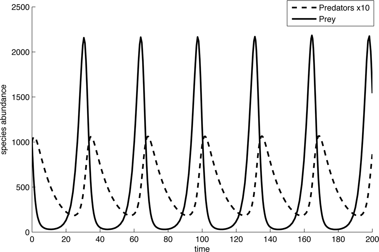
These equations describe a model which predicts one result: the predator and prey populations will oscillate indefinitely, out of phase with one another. Although for every set of parameter values with species coexistence, there exists one equilibrium where the populations do not oscillate, this equilibrium is unstable and hence a model population continues to oscillate if it is perturbed even slightly off of these equilibrium values.

Figure 1 plots the result of this oscillation for a set of parameter values and initial conditions. Qualitatively, it can be described as follows: As the prey population increases, the predator population increases as well, lagging behind. However, eventually, the predators begin to overtake the prey by continual feeding, which eventually begins to drive the prey population down in size. This results, in turn, in the predator population being driven down in size, and then the cycle repeats again. This undampened osscilation is the first important property of the L-V model that we will test for robustness in this paper. Before doing so, let us consider several more properties.

Figure 1.

Lotka-Volterra model's oscillation.

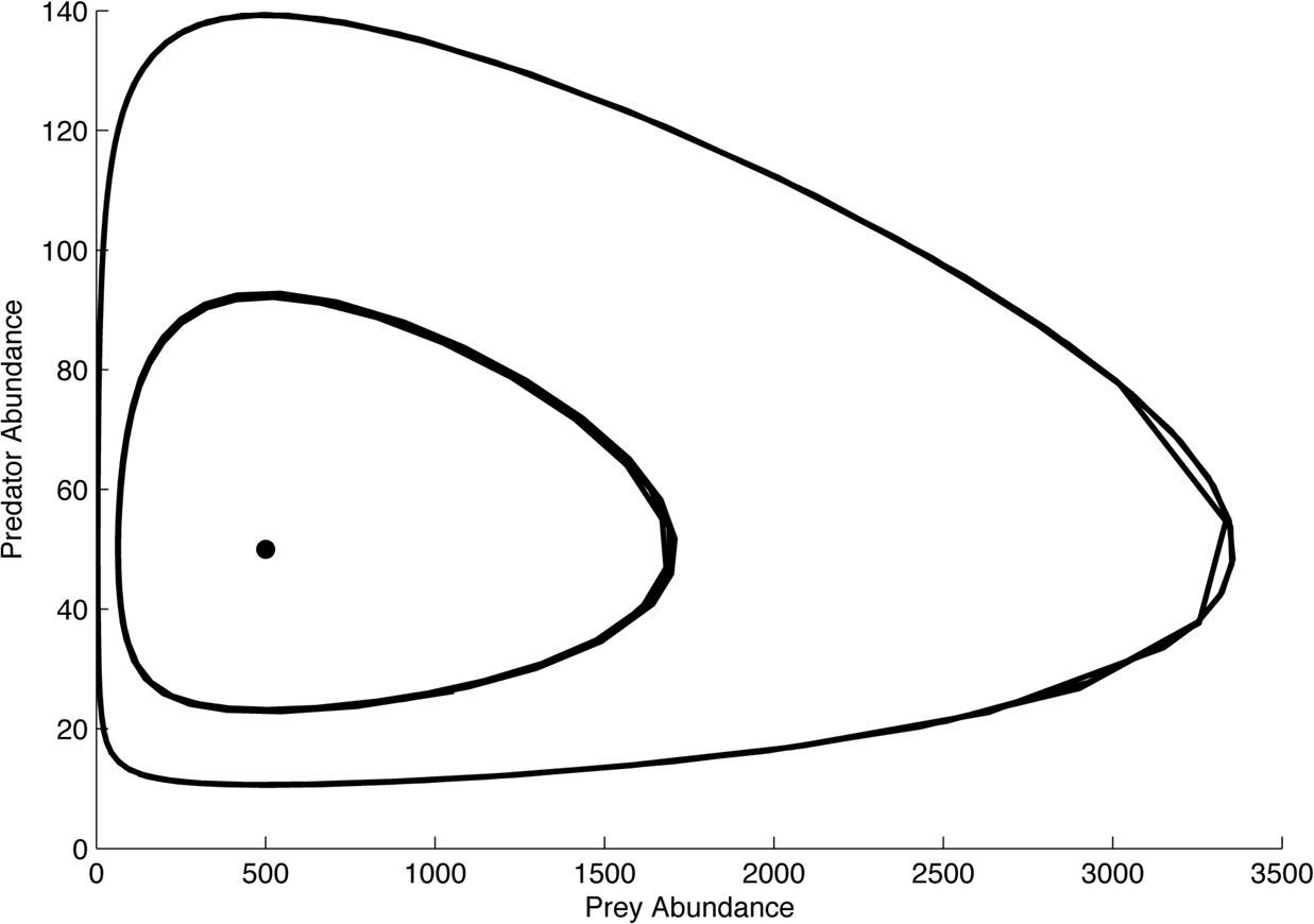
A second important property of the L-V model is neutral stability. The model exhibits neutrally stable oscillations, which means that perturbations away from the current oscillation amplitude will result in a new oscillation beginning from the point to which the oscillation was perturbed. There is no restoring force to bring the population back to the initial amplitude of the oscillations. This can be seen by plotting several trajectories, corresponding to different initial conditions, in the phase space of the model (see Figure 2). Each loop is closed, corresponding to a stable oscillation. Perturbation results in the formation of a new loop, corresponding to a new, neutrally stable oscillation.

Figure 2.

Phase-plot of Lotka-Volterra model.

The third and most important property of the L-V model is what we will call the Volterra Property, which is the key component of the Volterra Principle. The Volterra Property states that a general biocide, any substance which has a harmful effect on both predators and prey, will increase the relative abundance of the prey population. To see this, we first need to solve for the equilibrium abundances of the species by setting each differential equation to zero. After some algebra, we find that the equilibrium values are

These are unstable equilibria; however, they correspond to the average abundance of the predator and prey species over indefinitely long time periods.

We can derive the Volterra Property from the L-V model by first expressing the ratio of the average size of the predator population to the average size of the prey population ( $\hat{P}/\hat{V}$ ) as ρ. Decreases in ρ will correspond to increases in the relative size of the predator population.

From equations (6) and (5) we can see that

The next step is to consider how a general biocide affects the model populations. We can represent the introduction of a biocide as corresponding to changes in r and m. Specifically, biocides decreases the prey growth rate (r) and increases the predator death rate (m). Inspecting ρ, the expression for the ratio of average densities, we can see that $\rho ( \mathrm{biocide}\,) < \rho ( \mathrm{normal}\,) $ (Roughgarden Reference Roughgarden1997; May Reference May2001, 439). Since smaller values for ρ mean a larger relative size of the prey population, the population of prey will increase relative to the number of predators when a biocide is applied. This is the Volterra Property: the general biocide increases the relative size of the prey population.

The Volterra Property is a key component of the Volterra Principle, the ecological theorem alleged to be robust. The second component of the Volterra Principle concerns a particular kind of causal structure: negative coupling. A predator species and a prey species are negatively coupled just in case increasing the abundance of predators decreases the abundance of prey and increasing the abundance of prey increases the abundance of predators.

The full formulation of the Volterra Principle connects this core causal structure to the robust property as follows:

The Volterra Principle has great ecological significance. One very practical consequence of it is that pesticides will often increase unwanted pests, such as the effect DDT had on citrus groves in southern California in the 1950s. When it was used as a treatment against scale insects, orchardists learned that DDT makes the pest problem worse. The cottony cushion scale insect (Icerya purchasi) population increased upon the application of DDT because along with the scale insects, the DDT killed the vedalia beetle (Rodolia cardinalis), a predator species keeping the scale insect under biological control (Elton Reference Elton1958; Catagirone and Doutt Reference Catagirone and Doutt1989).

The principle also has a deeper theoretical significance. It provides a vivid example of how ecologically coupled systems can behave in unexpected, nonlinear ways. Interventions in such systems are difficult and, without due care, can have the opposite effect of what was intended.

3. Parameter and Structural Robustness

The three key properties of the Lotka-Volterra model—undampened oscillations (1), neutral stability (2), and the Volterra Property (3)—are very interesting and would be of great ecological relevance if they were generally true of real populations. One way to ask whether these properties hold generally would be direct empirical investigation. We could go out in to the field or design a laboratory experiment and see whether these predictions are close to what really happens. But there is another approach to answering the question, one that is often conducted prior to or in conjunction with direct empirical investigation. This approach is robustness analysis. If we investigate related but distinct models, do we continue to see these three properties?

The first step in answering this question is to examine a representative sample of the models described by equations (3) and (4). One does this by evaluating the behavior of the model under different parameter settings. This analysis ensures that there is no special dependence of an interesting result on some particular set of initial conditions. We call this kind of analysis parameter robustness analysis, because it shows us whether the model's behavior is dependent on any particular set of parameters. Parameter robustness analysis is also known as sensitivity analysis in the modeling literature.Footnote ⁴ Conducting parameter robustness analysis generates equivalence classes of parameter values that yield the same, or appropriately similar results.

Although we will not detail the analysis here, the three key properties of the L-V model are stable under wide ranges of parameter values for the L-V equations. In fact, as far as we know from surveying the literature and our own analyses, these three properties are robust across all parameter values where the two species coexist.

Parameter robustness can be applied alone when a theorist has good reason to believe that the basic structure of her model is adequate for her purposes, but remains uncertain about the values that should be assigned to the parameters. A second kind of robustness analysis relevant to our discussion of the Volterra Principle is what we call ‘structural robustness analysis’. In this kind of robustness analysis, the theorist considers changes to the causal structure of the system being modeled by analyzing models with a different mathematical structure. For example, in our model we might start with the L-V model, but add in terms representing predator satiation, the ability of prey to seek cover, multiple sources of food for the predator, or even complex adaptive behaviors such as learning. Any ecological interaction could in principle be added to the model.

Structural robustness analysis allows the theorist to address a different set of uncertainties from the ones addressed with parameter robustness. Using this approach, the theorist can probe which parts of the causal structure represented by her model are really essential for the production of an observed behavior of the model.Footnote ⁵ This can take the form of adding new components to the causal structure, where one starts from a very minimal model such as the L-V model and adds new causal interactions. It can also involve removing factors, such as when one starts with a complex model, calibrated to a particular system, and removes factors to see which ones really make a difference. Structural robustness thus helps theorists isolate which components are necessary for the production of an important property, and which ones produce less robust properties.

In the next section, we describe one kind of structural robustness analysis of predation models. We consider a density-dependent version of the L-V model, which builds in an environmental resource that limits population growth. This model makes a major structural change to the L-V model, but keeps the core negative coupling intact. We focus on this robustness test because density dependence has played a particularly important role in the development of predation theory.

4. Predator-Prey Model with Density Dependence

While considerations of structural robustness could lead us to add any additional function to the predator-prey equations, a natural ecological addition would be to add a carrying capacity to the growth rate of the prey. If the predators did not exist, this carrying capacity indicates the maximum size to which the prey can grow, typically limited by resources in the environment. Adding a form of carrying capacity can be accomplished by making the prey population growth density dependent. A logistic growth term of the form $dV/ dt=r( 1-V/ K) $ is substituted for the first term in the prey equation (Leslie Reference Leslie1948; Roughgarden Reference Roughgarden1997; Berryman Reference Berryman1992), yielding the following equations:

In the model described by these equations, there are three equilibria, which correspond to the three possible outcomes in the long run. The first equilibrium is extinction of both species. The second equilibrium involves predator extinction, but the prey continues to survive and grow to its carrying capacity. The third equilibrium is of most interest to us and says that both species can coexist. Solving these equations for this third, coexistence equilibrium, we get the following expressions:

Several things are worth noting about this equilibrium point. First and most important, it is a stable equilibrium; there are trajectories leading from the points in the vicinity of this equilibrium to this equilibrium. Once the populations settle on this point, they will not fluctuate in size unless they are perturbed. Population sizes in the vicinity of the other equilibrium values (full extinction or predator extinction) will likewise settle down to their respective equilibrium values.

The stability of this equilibrium can be demonstrated both analytically and graphically. Analytically, we can see that the equilibrium is stable by computing the eigenvalues of the Jacobian matrix. For all parameter sets that bring the population to the third equilibrium, the eigenvalues have a real part and the real part is negative. This corresponds to a stable equilibrium point (Roughgarden Reference Roughgarden1997; May Reference May2001).

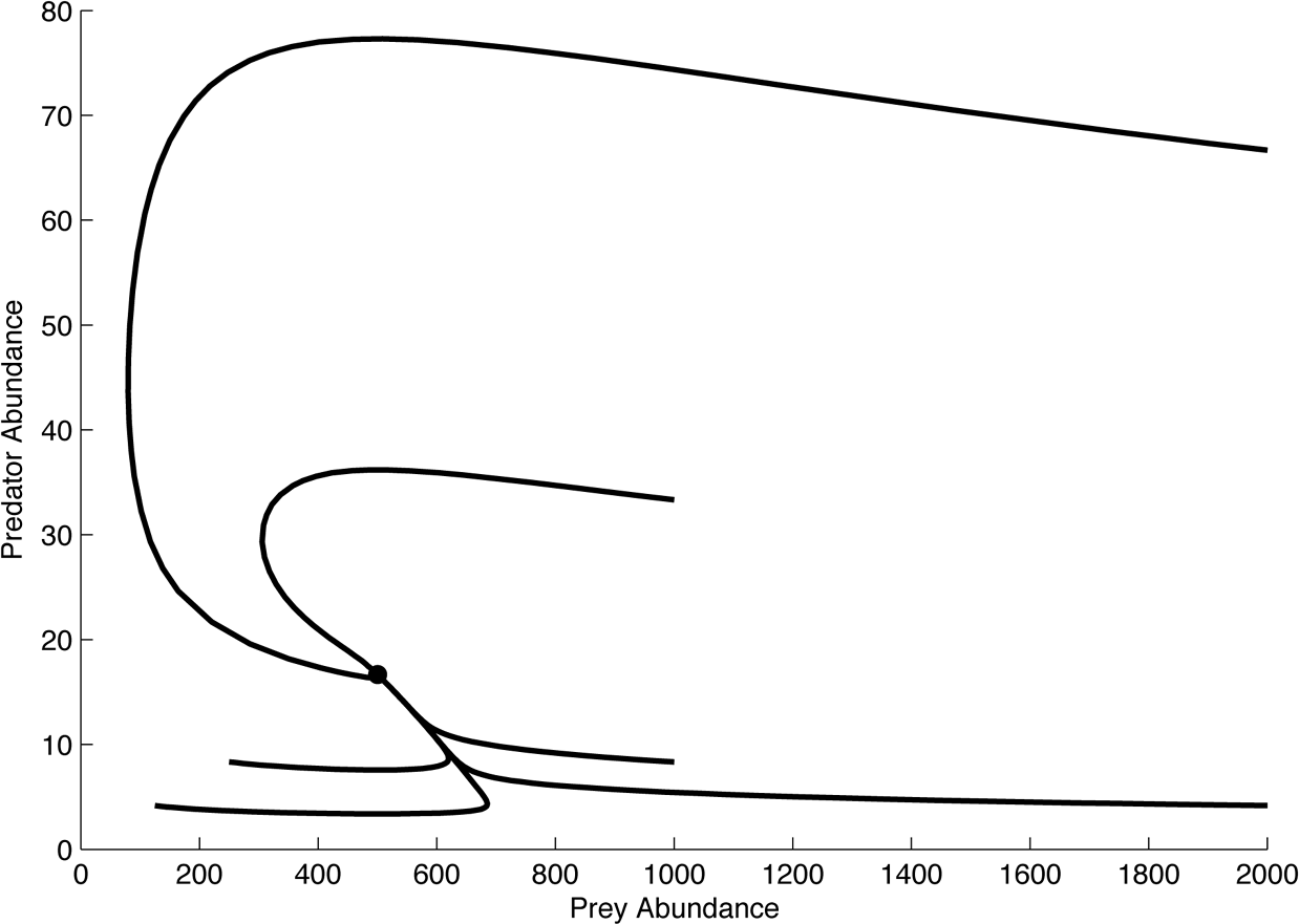
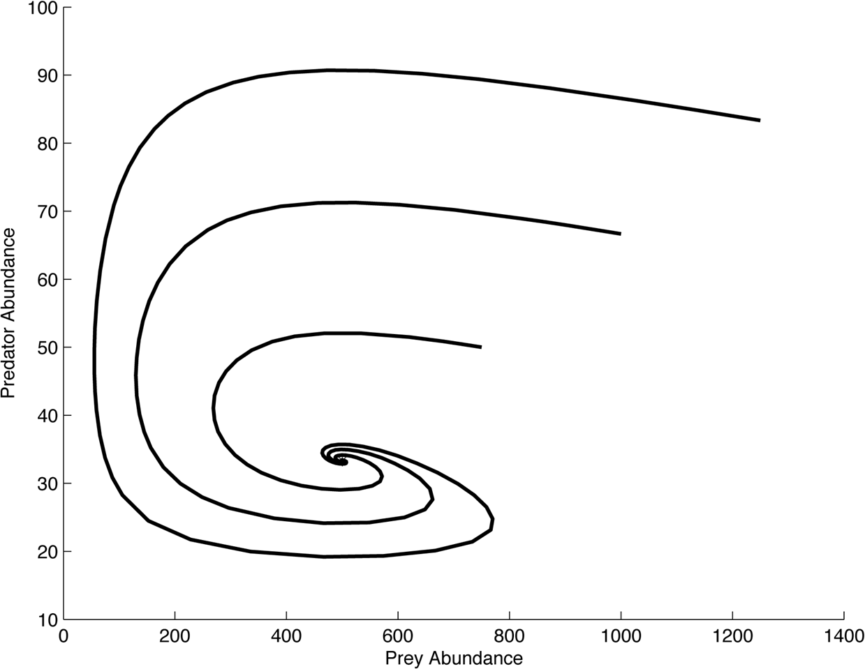
A graphical analysis is shown in Figures 3 and 4, which are graphs of the phase space for the density-dependent model with different values of K. In Figure 3, all of the trajectories can be seen leading in to the equilibrium point. In Figure 4, the trajectories spiral in to the point. The difference between these graphs is controlled by the magnitude of K. For smaller values of K, there is no oscillatory tendency in the approach to the equilibrium point. When K is larger, such as in Figure 4, the trajectories have an oscillatory tendency as they approach the equilibrium point. The oscillatory tendency increased in magnitude as K is increased. As $K\rightarrow \infty $ , the model becomes the L-V model and, as we would expect, the oscillations become undampened.

Figure 3.

Density-dependent Lotka-Volterra model with $K=750$ .

Figure 4.

Density-dependent Lotka-Volterra model with $K=1,500$ .

We are now in the position to make two comparisons between the density dependent model and the L-V model. The first property of the L-V model was undampened oscillations. In regions of state space where the density dependent model predicts coexistence, the model shows either no oscillations at all or dampened oscillations, all leading to a stable equilibrium. Even an arbitrarily small amount of density dependence will destroy the undampened oscillation. Thus the first property of the L-V model is not structurally robust and cannot be formulated as part of a robust theorem. Since the first property is not robust, the second property—neutral stability in the oscillations—cannot be robust either.

To examine the third property of the L-V model, the Volterra Property, we once again express the coexistence equilibrium values as the ratio ρ, yielding

Since r is in the numerator and m is in the denominator, we can see that the Volterra Property, and by extension the Volterra Principle, holds for this model. If we increase the death rate of the predators and decrease the growth rate of the prey, this corresponds to smaller values of ρ, meaning the relative size of the prey population increases. In fact, in this model the Volterra Principle has an even more direct interpretation. In the L-V model, the equilibrium values corresponded to the average size of each population. However in the density-dependent model, the terms in ρ are the actual equilibrium abundances of the two populations. Decreasing ρ will have a direct effect on the equilibrium size of the populations, not the average size over time.

Further structural robustness analysis would consider other changes to the causal structure represented in the model drawn from the kinds of ecological factors known to be relevant to population dynamics and predation. While any change to the basic structure is a kind of structural robustness test, ecologists are most interested in the ones that are potentially ecologically realizable. When a robust property survives all or some range of structural robustness tests, then we can say that the property is structurally robust to such and such changes to the causal structure of the system. If these changes sample a sufficiently broad set of ecologically plausible circumstances, then ecologists will often simply refer to a phenomenon as robust.

5. Representational Robustness

Testing the structural robustness of a theorem is a matter of iteratively varying the basic assumptions of a model to see whether the theorem continues to hold. We could make many other modifications to the density-dependent predator-prey model to test the structural robustness of the L-V model. For example, we might examine other equations for the functional and numerical responses, examine the effects of population stochasticity, include the possibility of predator satiation, and add terms describing the prey's ability to hide from the predators. These possibilities were explored and shown to be robust in the classical ecology literature about predation.Footnote ⁶ Instead of following those analyses here, we now turn to a different kind of robustness, which varies what we will call the representational framework of the model.

Mathematical models can be thought of as being composed of state variables, which are variables that represent the properties (states) of interest to the modeler and transition rules, the rules that govern how the states change through time (Lewontin Reference Lewontin1963). The representational framework of the model is a general description of the type of state variables and the type of transition rules the model employs. For example, the variables in a biological model might represent individuals or populations. They might also represent more abstract properties of target systems, such as energy or nutrients, or even pathways by which these properties flow. Transition rules can be deterministic, probabilistic, or stochastic. They can also be discrete or continuous with respect to time.

The models we have considered so far use population densities as their state variables and have deterministic transition rules that are continuous with respect to time. Thus they were formulated using a set of differential equations. Versions of these models that use difference equations could very easily be generated, which would make them discrete with respect to time but hold the other aspects of the representational framework constant. Further changes can be made by adding in probabilistic transition rules or changing the perspective of the state variables from populations to energy flows or to individual organisms.

Parameter and structural robustness analysis vary assumptions about the target phenomena to see how the emergence of the phenomenon is sensitive to these assumptions. Representational robustness analysis lets us probe a different feature of our models. It holds these assumptions fixed, but analyzes whether or not the way these assumptions are represented make a difference to the production of a property of interest.

Recent ecological literature has been especially concerned with the representational robustness of classic population based models when they are reconstructed in an individual-based framework, where the state variables are attached to individual organisms (Grimm and Railsback Reference Grimm and Railsback2005). In the next sections, we illustrate representational robustness analysis by considering two novel individual-based models of predation with which we tested the Volterra Principle for representational robustness.

6. Individual-Based Predator-Prey Models

The models considered so far have treated predation as a population-level phenomenon. These models aggregate the properties of many organisms and represent them using just a handful of population-level state-variables. They contain no explicit representation of individuals or their properties, only the statistical aggregates of those properties. In contrast, individual-based models (IBMs) explicitly represent individuals and their properties. An IBM includes a set of state variables for each individual within the model population. It also include assumptions about how individuals in the population behave, develop, and interact over time. Since IBMs often contain thousands of variables, their dynamic consequences are usually investigated via computational simulation rather than mathematical analysis.

Population-level models are often more elegant and amenable to mathematical analysis than IBMs, but their very simplicity can be limiting. Ecological systems have rich structure that is not readily visible from a population-level perspective. Organisms within a population generally differ in their properties and life histories. Interactions between organisms are local, involving a few individuals at a particular place and time. IBMs are effective at capturing this individual-level detail because they explicitly represent the properties of each organism in a population, and because individuals can be set up to interact in small numbers on a spatial lattice. When one wants to test whether individual variability or local interactions affect the robustness of a generalization, one can build an IBM.

IBMs are also useful because they integrate our understanding of the different levels in the biological hierarchy. Ecologists gather data about organisms, populations, and communities. IBMs help reconcile these multiple levels of data, because assumptions about organisms and their interactions enter into an IBM, and the population or community consequences of these assumptions result from running IBM simulations. IBMs are thus informed and constrained by ecological data at multiple levels. In contrast, the points of contact between population-level models and data are all at the population and community levels. Such models include assumptions about populations, but they are either silent or ambiguous concerning assumptions about individuals. This can be a strength when we want to remain agnostic about those assumptions, but it can also be a liability. In many cases, we may want to vary those assumptions and understand their consequences.

In recent years, IBMs have become increasingly common within ecology and among the sciences more generally. (See also Donalson and Nisbet Reference Donalson and Nisbet1999; DeAngelis and Mooij Reference DeAngelis and Mooij2005; Grimm and Railsback Reference Grimm and Railsback2005.) They are not a substitute for population-based models, but they can be used to relax assumptions made by generating population-based models. As such, each of these frameworks may be more or less appropriate depending on the purpose at hand. Indeed, for the purpose of testing the robustness of a generalization, one ought to examine as many representational frameworks as possible.

To test the representational robustness of the three key properties of the L-V model, we will translate its variables, parameters, and other assumptions into individual-based terms.Footnote ⁷ In our discussion of the L-V model, we showed how the model makes assumptions about the growth and death rates of the predator and prey populations and about the interaction between these populations in the form of predation. Any individual-based version of this model must reconceive these processes in terms of individuals; it must make assumptions about the births and deaths of discrete predator and prey individuals, and the interactions between these discrete individuals in the form of predation.

In our first IBM version of the L-V model, we assume that individuals move about on a $30\times 30$ toroidal lattice composed of 900 cells. Each individual has three variables: a binary variable denoting whether the individual is predator or prey, and two integer variables denoting a vertical and horizontal position on the lattice. Time is discrete; a global clock advances one tick at a time. For each tick of the global clock, all individuals execute a fixed set of rules that determine how they move on the lattice, reproduce, die, and interact with others. The rules for predators are as follows:

These rules, when executed by each predator on the lattice, correspond roughly to assumptions made in the L-V model, but notice that these rules are not determined by that model. To translate any population-based model into individual-based terms, we must make explicit assumptions about individuals that were either implicit or undefined in the population-based version. This means that there is typically no uniquely correct way to carry out the translation from population-based to individual-based models.

The IBM assumes that predators move randomly on a two dimensional toroidal lattice. The L-V model, on the other hand, makes no assumption about movement at all. It is consistent with the assumptions that all individuals move, that some individuals move, or even, strictly speaking, that no individuals move. It places no explicit constraints on what intrinsic or environmental factors determine movement or even whether the predator and prey move in a probabilistic or deterministic fashion.

Moreover, the IBM assumes that predators catch prey by randomly selecting one prey individual from all that are located on the same cell. Once again, this is one of the many possible assumptions we could have made to develop an IBM analogue of the L-V model. We could have represented predation without using a spatial lattice, where predators randomly choose prey individuals from the whole prey population. We could also have used a different predation rule on a lattice. For example, the predation rule could have stated “if a predator is within 1 cell of a prey, then the prey is consumed.” The L-V model does not strictly correspond to any of these particular assumptions. A modeler who wishes to construct an IBM, however, must make an explicit decision about them.

Our corresponding rules for the prey are as follows:

Together, the predator and prey rule-sets comprise one possible IBM interpretation of the L-V model. Notice that, as with the L-V model, this IBM defines a negatively coupled predator-prey system. Ceteris paribus, increasing the abundance of predators in the IBM will increase the chance that prey are captured, and thus decrease the expected number of prey. Ceteris paribus, increasing the abundance of prey will increase the chance of a predation instance. Since each such instance has a fixed probability of resulting in predator reproduction, increasing the abundance of prey will increase the expected number of predators. It is critical that the IBM does indeed define a negatively coupled system, because negative coupling is a necessary condition for a system to demonstrate the Volterra Principle.

To understand the dynamic consequences of this model, we set up a computational representation of a lattice, place predator and prey individuals on the lattice, iteratively execute the predator or prey rules for each individual, and observe how the system evolves over time. In the initial state used in our simulations, there are V prey and P predators positioned randomly on the lattice.

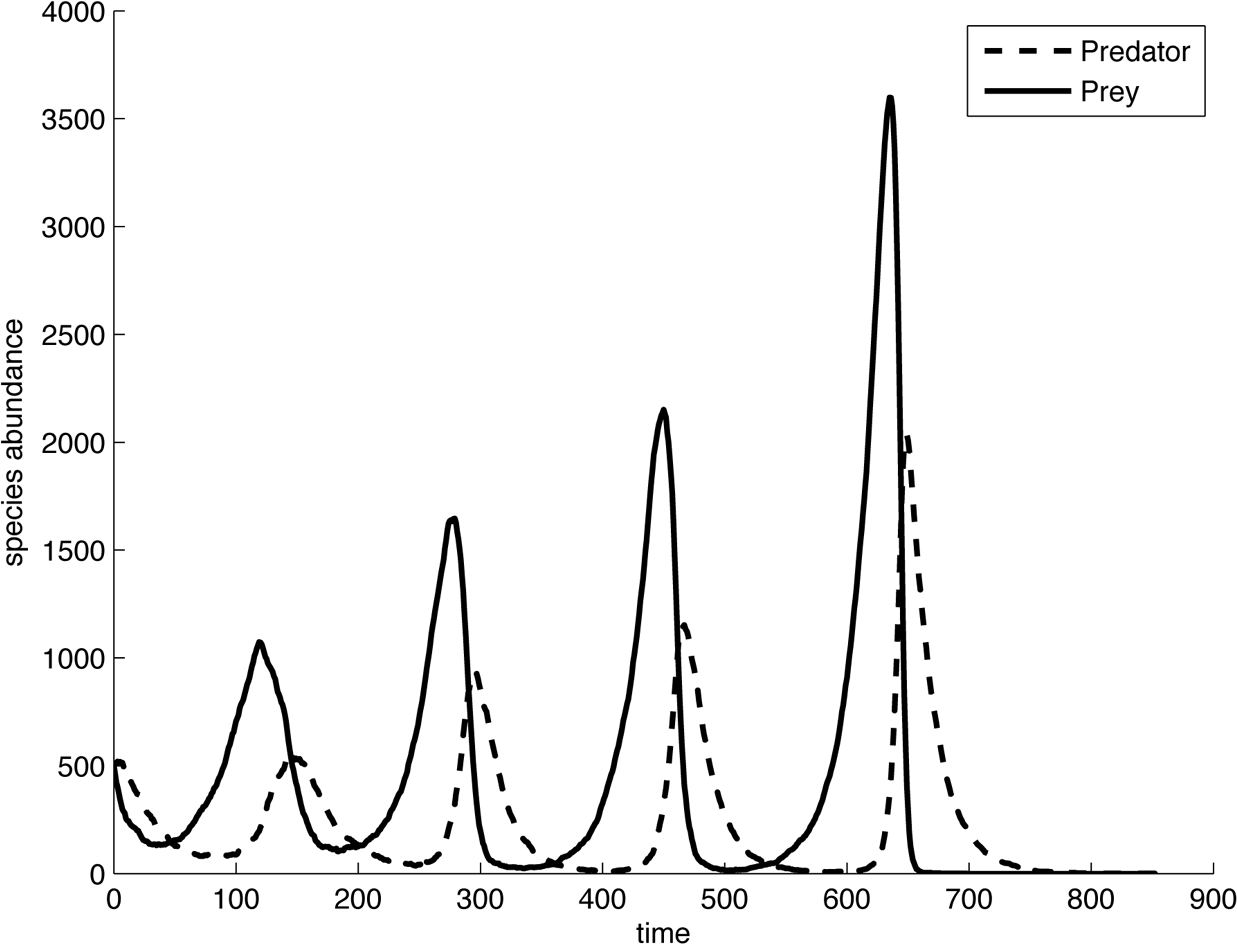
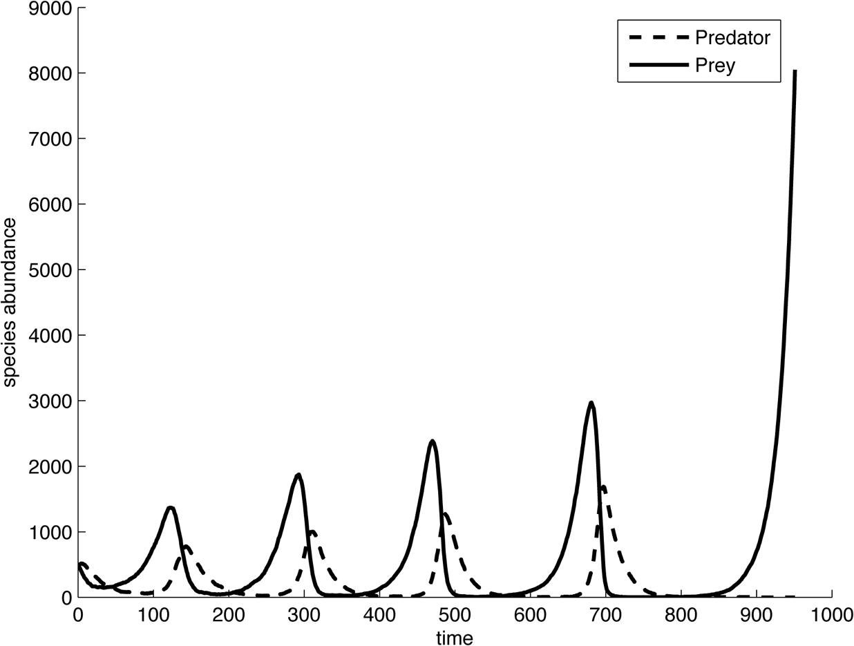
After observing many simulations with differing parameter sets and initial conditions, we concluded that this IBM does not exhibit stable oscillations in the numbers of predators and prey, the first property of the L-V model.Footnote ⁸ There are sets of parameters which initially result in oscillations, but these oscillations are unstable, increasing in amplitude over time until either both species have gone extinct (Figure 5), or else the predators have gone extinct and only the prey remain (Figure 6). Because this is a probabilistic model, the same parameter set and initial conditions sometimes results in two-species extinction and sometime results in the prey surviving. Figures 5 and 6 correspond to this situation: both used the same parameter set and initial conditions.

Figure 5.

Simple individual-based model corresponding to the Lotka-Volterra model. In this trial, both species go extinct.

Figure 6.

Simple individual-based model corresponding to the Lotka-Volterra model. In this trial, only the predators go extinct.

Regardless of the parameters, one or both species invariably goes extinct. This result suggests that stable oscillations, or even stable coexistence, is not a representationally robust feature of predator-prey systems. Since the IBM does not exhibit stable oscillations, it clearly will not exhibit property 2 of the L-V model, neutrally stable oscillations.

Finally, since the IBM does not exhibit coexistence of species, even in the short or medium term, it cannot exhibit the Volterra Property. Testing this property requires examining the effect of a biocide on average abundances, which are either $\hat{P}=0$ and $\hat{V}=\infty $ or $\hat{P}=0$ and $\hat{V}=0$ for this model. Coexistance of predator species is a precondition for the Volterra Principle to hold. To test the representational robustness of this property and the Volterra Principle itself, we must begin with a predator-prey model which has quasistable behavior for a reasonable length of time.

Since we would like to test for the robustness of the Volterra Principle, we need to find an IBM that exhibits coexistence of the two species. In the next section, we describe a modification that does stabalize the populations. It acheives this stabalization by adding density-dependence.

7. Density Dependent IBM

One source of instability in the previous model is the lack of limits on population growth. The population oscillations tend to become more pronounced with each successive cycle until the population of one or both of the species falls too low and the species goes extinct. This suggests that if we introduce a carrying capacity to limit the upward amplitude of the oscillations in this model, extinction will be less likely.

How can we impose a carrying capacity on the model? The most direct way is to assume a fixed global limit on the number of predators and prey, yet this is not in the spirit of individual-based modeling; it is a top-down assumption about populations, rather than a bottom-up assumption about individuals. A bottom-up alternative is to impose a limited resource into the model, such as space. For example, we might assume that at most one predator can occupy any cell in the lattice at a given time.Footnote ⁹ Another type of limited resource is food for the prey population. For example, if the prey are herbivores, the limited availability of edible foliage in the environment imposes a natural carrying capacity on the prey.

In our density-dependent IBM, we assume that the size of the prey population is limited by availability of food in the environment (for convenience, we will call the food ‘foliage’, but it could represent any naturally available resource). We assume that each cell of the lattice either contains a unit of foliage or not. When eaten by a prey individual, the unit of foliage disappears, and it then has a certain probability (set by the parameter foliage-growth-prob) of reappearing at any subsequent tick. These assumptions suggest a revised rule-set for prey with a new foliage rule and a revised death rule:

The rule-set for predators remains the same.

Does this modified IBM, with density-dependence, display any of the three basic properties of the L-V model discussed earlier? After investigating many different initial states and parameter sets, we concluded that there is a wide range of parameter conditions for which this model does exhibit oscillations in the numbers of predators and prey for very long periods of time.Footnote ¹⁰ The amplitude of the population oscillations tends to vary stochastically over time, but both species do persist and oscillate for long runs of the model.Footnote ¹¹ Thus, the density-dependent IBM exhibits an analogue of property 1 of the L-V model; for very long time intervals, it exhibits undampened osscilations.Footnote ¹²

The model does not appear to exhibit property 2, neutrally stable oscillations. Under all the conditions we examined which result in stable oscillations, the average abundance of predators and prey did not depend upon initial conditions or prior population sizes. After perturbing the populations away from their equilibrium temporal average sizes, the populations would always return to their former averages. This suggests that property 2 of the L-V model is not representationally robust.

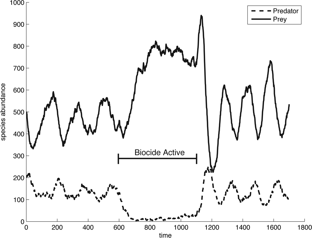
To check whether the model exhibits the Volterra Property, we must somehow simulate the effect of a general biocide that would elevate the death rate of both the predators and of the prey. Since there are no parameters in the model that correspond directly to these rates, we must manipulate them indirectly. Fortunately, the individual-based framework makes it easy to simulate the dispersion of a general biocide into our model system. We performed the following perturbation: First, initiate a typical simulation of the predator-prey system and wait long enough for the temporal average size of each population to reach a steady state. Next, randomly select some cells on the lattice to become ‘poisonous’, so that any predator or prey that lands on the cell will die. Since movement is random, predators and prey are equally likely to die as a result of landing on poisonous cells and the result is an increase in the death rate of both populations. Finally, wait for the temporal average size of each population to reach a new equilibrium.

After performing this perturbation over a broad range of parameter settings,Footnote ¹³ we found that introduction of a general biocide tended to increase the average size of the prey population and to decrease the average size of the predator population (Figure 7). Thus, this revised IBM does exhibit the Volterra Property. Moreover, since this model also defines a negatively coupled predator-prey system, it satisfies the Volterra Principle. In other words, despite moving from a population to an individual-based framework, and despite altering various assumptions of the L-V model, the Volterra Principle still held up. This suggests that it is representationally robust.

Figure 7.

Density-dependent individual-based predation model with biocide perturbation.

The analyses in this paper show that the Volterra Principle exhibits three kinds of robustness. Naturally, the scope of the Volterra Principle's robustness is not a settled matter. Analysis could continue with different and more realistic models. For example, we might investigate a model where reproduction and death are tied only indirectly to food consumption via the introduction of rudimentary elements of metabolism.Footnote ¹⁴ In fact, tests for robustness are always an ongoing matter. It is unlikely that a theoretical community will settle the issue of a theorem's robustness once and for all.

8. Conclusion

Volterra discovered the principle which bears his name in 1926. By constructing a series of models, all similar but differing in some respects, ecologists have shown that the Volterra Principle is robust and accurately describes a real ecological phenomenon—when two species in a negatively coupled, predator-prey relationship coexist, a general biocide will favor the prey over the predators. In our discussion of four models of predation, we have outlined three kinds of robustness analysis which correspond to three different levels at which a result's robustness can be determined in modeling. These are parameter robustness, a result's surviving changes to the parameter set of a dynamical model; structural robustness, a result's surviving changes to the mathematical structure of the model; and finally, representational robustness, a result's surviving changes to the whole representational framework in which the model has been framed. Like all of the most important robust theorems, the Volterra Principle possesses all three kinds of robustness.

Robustness analyses of the Volterra Principle carried out by the ecological community, as well as the novel representational robustness analysis carried out in this paper, has several implications. Most importantly, robustness analysis has shown that the principle is highly general and will hold under a wide variety of conditions. It is not dependent on idealizing assumptions made in various models of predation. While any given model contains idealizing assumptions, analysis across models has allowed us to control for them and factor them out. The principle is also insensitive to many other detailed assumptions made in the modeling process (for example, concerning the mode of animal movement, reproduction, metabolism, etc.) This insensitivity to detail helps explain why the Volterra Principle has been confirmed in widely disparate natural systems, from cottony cushion scale insects and vedalia beetles to cod, Norwegian lobster, and sharks. In contrast, robustness analysis has revealed that several other properties of the original Lotka-Volterra model, including stable oscillations and neutral stability, are not robust in this respect.

Levins (Reference Levins and Sober1966, 20) wrote that “our truth is at the intersection of independent lies.” We do not see models, even the highly idealized ones involved in the robustness analysis of the Volterra Principle as ‘lies’, yet we think Levins’ point is correct. When studying phenomena as complex and hard to measure as predation, scientists often have little choice but to build approximate, idealized models. Finding that some result is robust across these models, however, is an important step in the process of a theorem's confirmation.