1. Introduction
Since there is a strong relationship between climate and glaciers, and our information about glaciers covers a much longer period than direct meteorological measurements, it is tempting to try to use glacier observations to investigate the past climate.
However, moraines and historical documents usually tell us about cold times, when glaciers were large, but little or nothing about the warm phases in between. The behaviour of the glacier must therefore be simulated over the whole time period we want to investigate. The results have to be controlled at certain points using moraines and old maps. A successful glacier simulation with proxy data could then enable us to estimate temperature or precipitation during that period.
Several authors have tried to simulate historical front positions of different Alpine and Scandinavian glaciers (e.g. Smith and Budd, 1981; Greuell, 1989; Stroeven and others, 1989), but in most cases results were unsatisfactory, which, according to the authors, is due to insufficient climate data.
A central flowline model was adapted to reconstruct fluctuations of Hintereisferner, a well-studied glacier in the Austrian Alps, since the last postglacial maximum in the mid-l9th century.
2 The Model
2.1. Basic equations
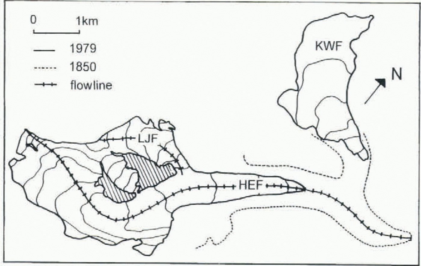
The model used here is based on a model of Greuell (1989), which is similar to models developed by Oerlemans (e.g. Oerlemans, 1986) and Budd (e.g. Smith and Budd, 1981) and their co-workers. It is a one-dimensional (central flow-line) model, with x as the variable in flow direction. The three-dimensional geometry of the glacier is parameterized assuming a trapezoidal cross-section. Figure 1 shows Hinter-eisferner with its two tributaries, Langtaufererjochferner and Kesselwandferner, and the corresponding flowlines. The grid-point distance is 200 m. Ice-thickness changes and ice velocities are calculated along a central flowline.
The change of cross-sectional area (and therefore, with simple geometrical considerations, the change of ice thickness) with time can be described by the continuity equation:

where S is the cross-sectional area, ū is the mean cross-sectional velocity, m is the mean specific mass balance, and B s is the glacier width at the surface.
The velocity is the sum of deformation velocity u d and sliding velocity u s The deformation velocity is calculated here as follows:

where S 1 is the shape factor, S 2 is the ratio of mean cross-sectional
Hintereisferner (HEF) with its tributary Langtaufererjochferner (LJF) and its former tributary Kessel-wandferner (KWF) and the flowlines used in the model.

velocity to surface velocity, f 1 is the “flow parameter”, H is the ice thickness, and τ b is the basal shear stress.
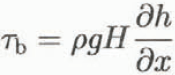
where ρ is the ice density, g is the acceleration of gravity, and h is the surface elevation.
s 1 takes into account friction at the valley walls. In the original version by Nye (1965), s 1 is used as a factor in Equation (3) for the basal shear stress. However, there are inevitable errors in the determination of s 1. Due to the high exponent of the basal shear stress, not only s 1 but also this error would be taken to the third power, which is very problematic for the numerical simulation. Thus, in this case the shape factor is only put into the equation for the deformation velocity, in order to keep its x dependence without influencing the model results too strongly.
The sliding velocity depends strongly on the basal water pressure, which unfortunately is not known and cannot be calculated convincingly either. Since it does not make sense to use a complicated equation to describe a physical process which is not really understood, in this case a simple sliding law is used. A commonly used equation is (Paterson, 1994):

where f is a “glacier specific parameter”, an adjustable parameter which depends on the mechanical and thermal properties of the ice and on the characteristics of the bed, N is the overburden load, and p is the basal water pressure.
Since we do not know the basal water pressure, formally a fraction of the overburden load instead of the effective pressure is taken in the denominator in Equation (4) (assumption: q = 1, n = 3):

(The factor 0.5 might as well have been included in f 2, but it should indicate, formally, how the equation was derived.) f 1 and f 2 are used as tuning parameters.
To ensure numerical stability an “upstream differencing” scheme in space and a simple forward scheme in time are used.
The model does not contain longitudinal stress gradients explicitly. Nevertheless they are taken into account by averaging the basal shear stress longitudinally with a triangular weighting function (Kamb and Echelmeyer, 1986).
2.2 Mass balance
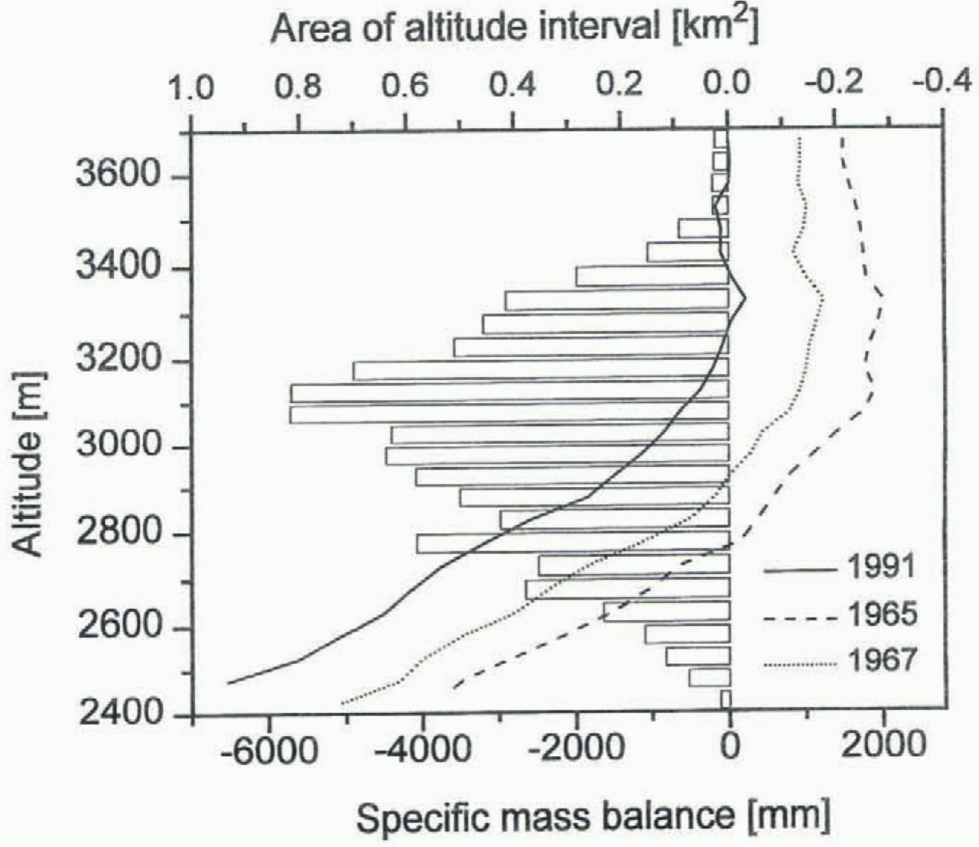
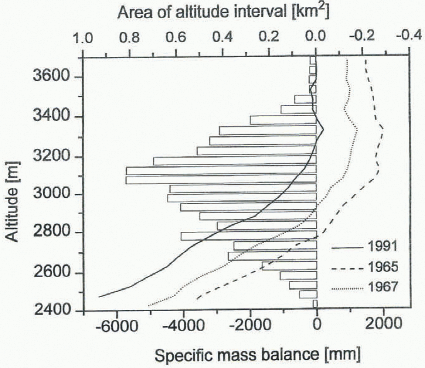
As forcing function for the model the specific mass balance is used. The treatment of the mass balance, especially its dependence on altitude, is extremely important for the success of the modelling. Figure 2 shows the specific mass balance of Hintereisferner vs altitude for different years. It can be clearly seen that the curves are nearly parallel. Therefore the mass balance can be considered as the sum of a time-independent but altitude-dependent term and an altitude-independent term, which varies from year to year (Lliboutry, 1974; Kuhn, 1984):

The last term on the righthand side of the equation represents the irregular change of the mass balance plus the remaining error due to errors in measurement or analysis.
Specific mass-balance–altitude curves of Hintereisferner for different years. Note that all curves are nearly parallel.
Since neither is considered in the model they are written here as one term.
In order to obtain a “reference” mass-balance–altitude curve, first the mean specific mass balance for the period 1961–91 was calculated for each 100 m altitude interval. Then the shape of the curve was optimized empirically, so that for the calibration period the best agreement between model result and observed change was achieved.
To calculate the specific balance of a certain altitude in the model, this reference curve was shifted by the difference between specific mass balance of the simulation year and specific mass balance of the reference curve.
3 Data
3.1. Topography
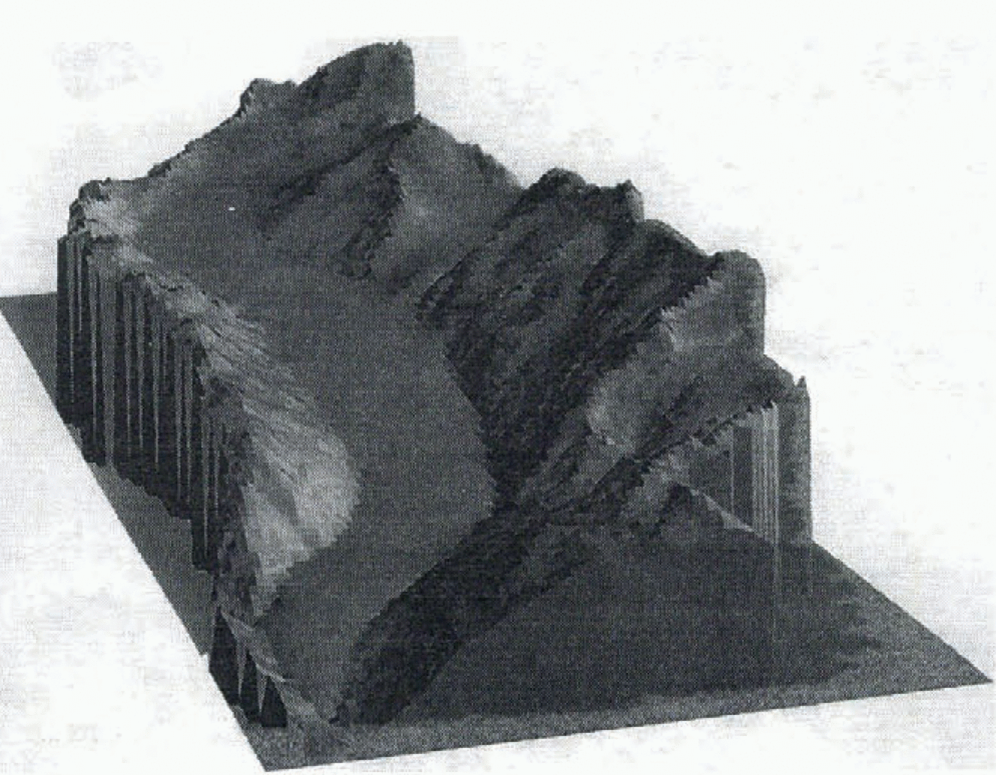
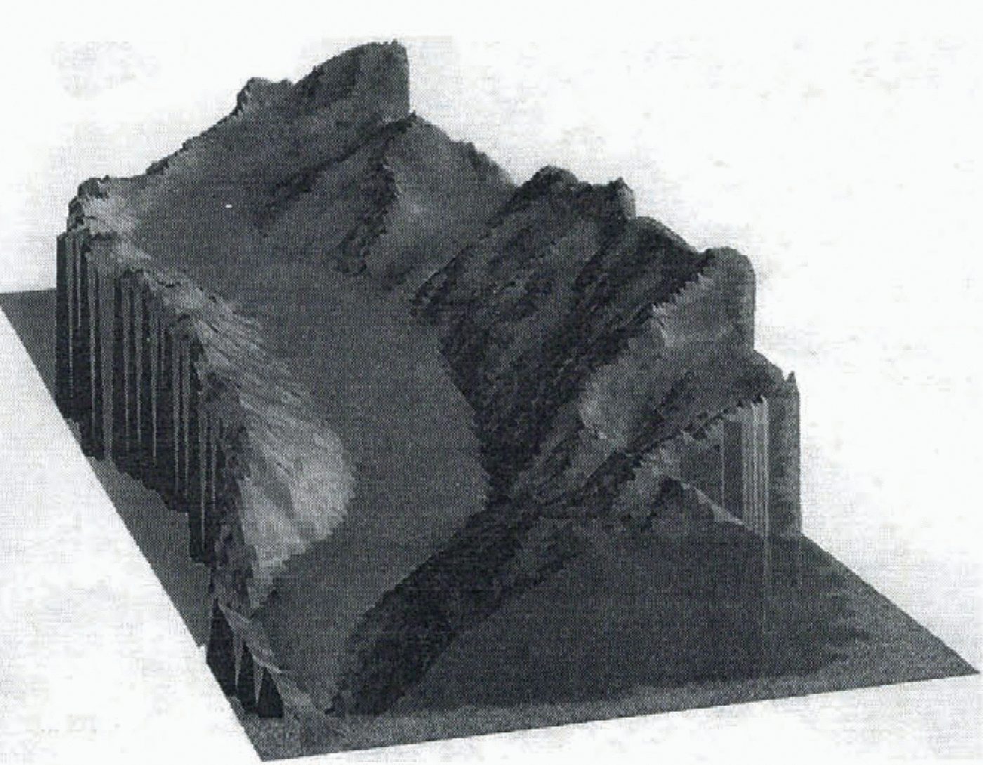
The oldest map of Hintereisferner is from 1894, the most recent one from 1979. For the simulation, maps of 1920 and 1953 were also used. A map for the Last Glacial Maximum about 1855 was reconstructed using moraine evidence. A digital terrain model of the reconstruction is shown in Figure 3. From this reconstructed map the initial ice thickness
Digital terrain model of the reconstructed Hintereisferner in 1855.
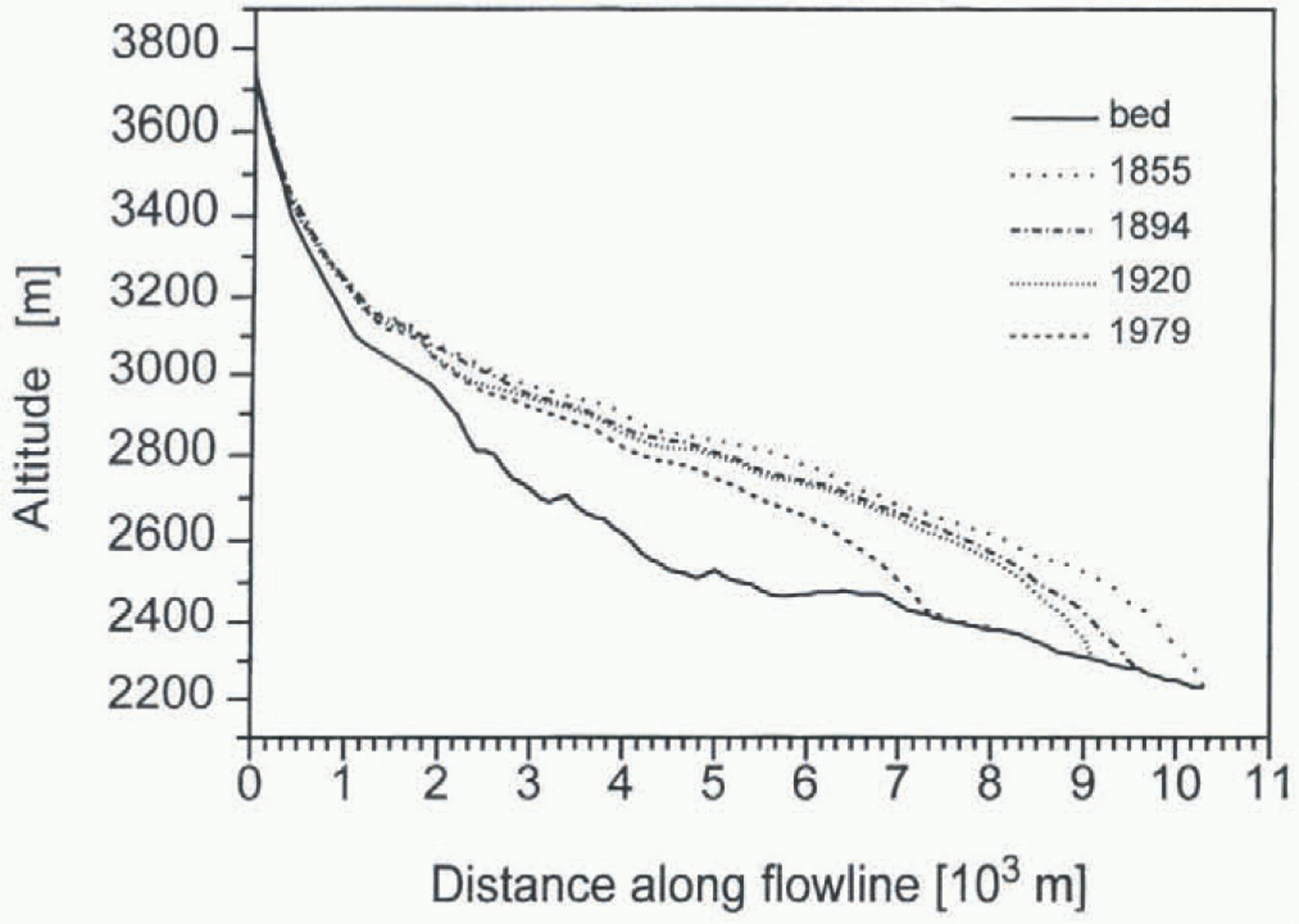
Longitudinal ice thickness profiles of Hintereisferner for 1855, 1894, 1920 and 1979.
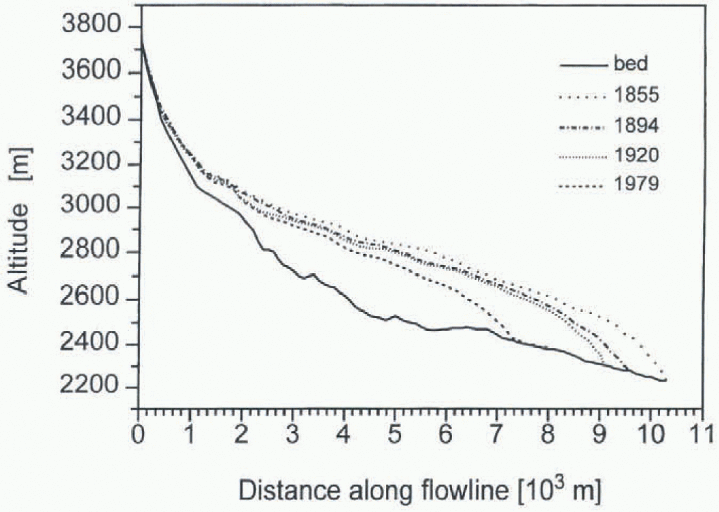
profile for the model runs starting around 1855 was obtained. Figure 4 shows the thickness profiles for 1855, 1894, 1920 and 1979. The bed was mainly known from radar measurements carried out by H. P. Waechter in 1982 (unpublished report). For the upper part of the glacier the bed had to be estimated from the surface slope, assuming a basal shear stress of 105 Pa.
3.2 Mass balance
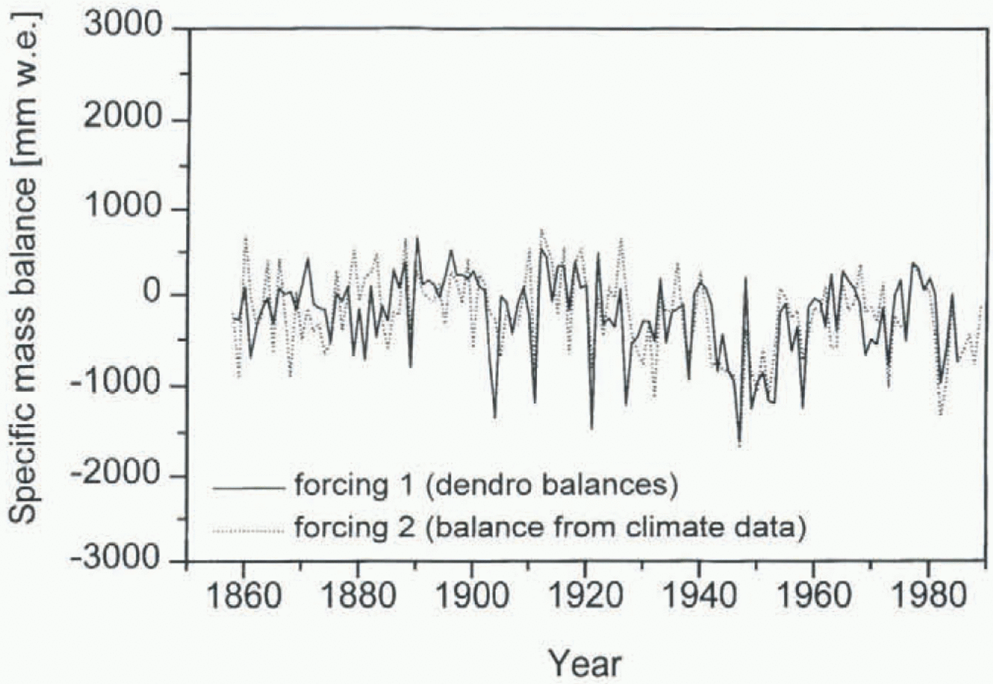
Since 1953 the specific mass balance of Hintereisferner has been determined using the direct glaciological method (Hoinkes, 1970), which makes this mass-balance series the longest in the Eastern Alps, the third longest worldwide. For the period before 1953 the mass balance was calculated in two different ways: Nicolussi (1995) derived the mass balance directly from tree-ring widths he got from trees at the timber line in the vicinity of Hintereisferner. This series of so-called dendro-mass balances goes back to 1386, the age of the oldest wood found close to Hintereisferner. (These are the oldest available proxy data and might help to extend the simulation beyond 1850 once the other problems mentioned below are solved.) In addition, the mass balance was parameterized as a function of temperature and precipitation from two adjacent climate stations, Vent (16 km northeast of Hintereisferner) and Marienberg (19 km southwest of Hintereisferner). The precipitation series of Marienberg starts in 1858; temperature at Vent has been measured continuously since 1934; earlier, intermittent records have been completed with data from other climate stations back to 1850. The best correlation (r = 0.77) between mass-balance and climate data was achieved using the weighted summer temperature ((0.5T May + T June + T July + T Aug + T Sept)/4) of Vent and winter precipitation (October–April) of Marienberg.
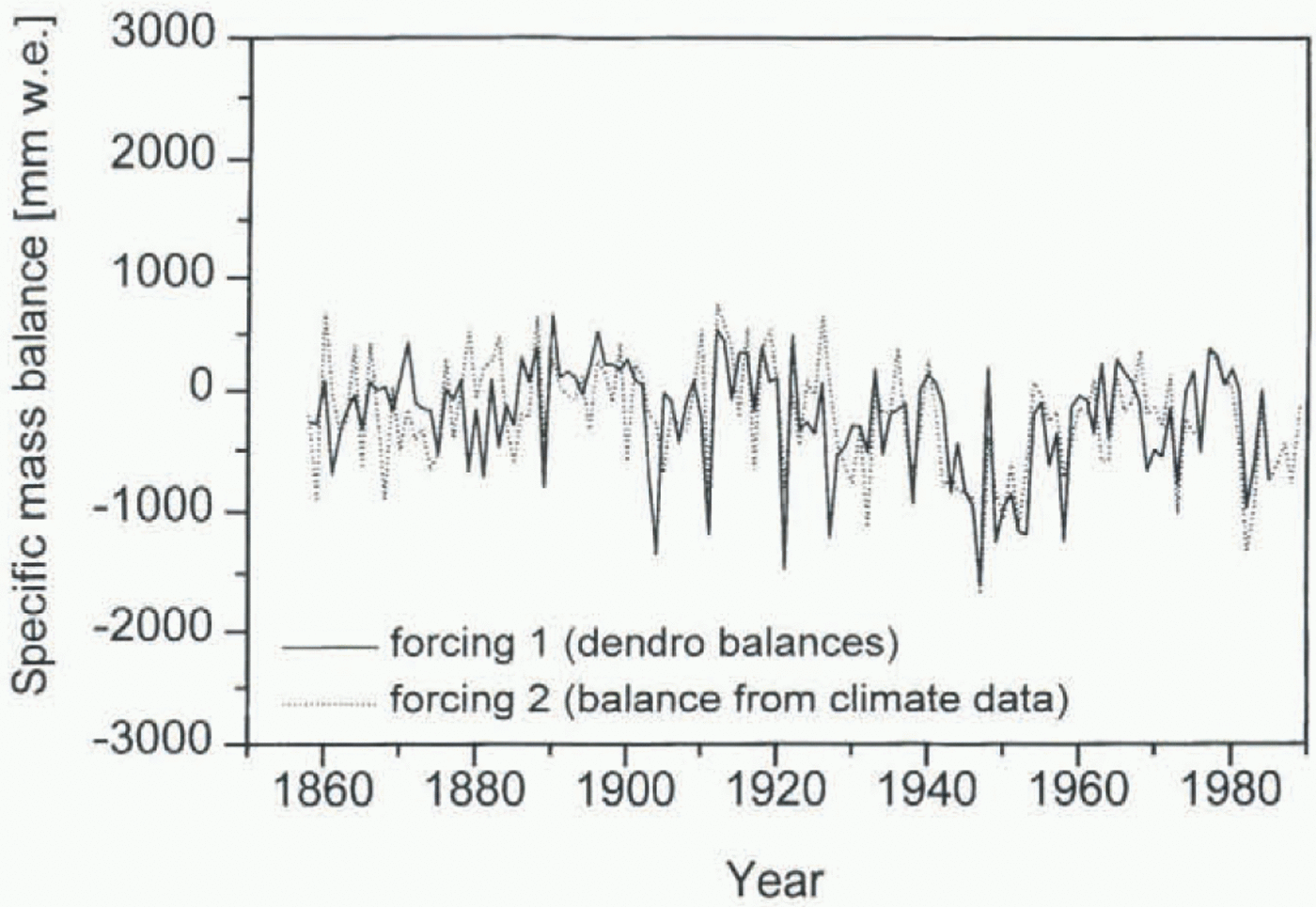
Figure 5 shows the two forcing functions for the simulation 1858–1979, the dendro-balances and the balances calculated from climate data.
4 Calibration
The model was calibrated with the period 1953–79, because the mass-balance series of Hintereisferner begins in 1953 and the most recent map is from 1979.
Forcing functions for the simulation 1858–1979: 1. dendro-mass balances (derived from tree rings); 2. specific mass balance calculated as function of temperature and precipitation from adjacent climate stations.
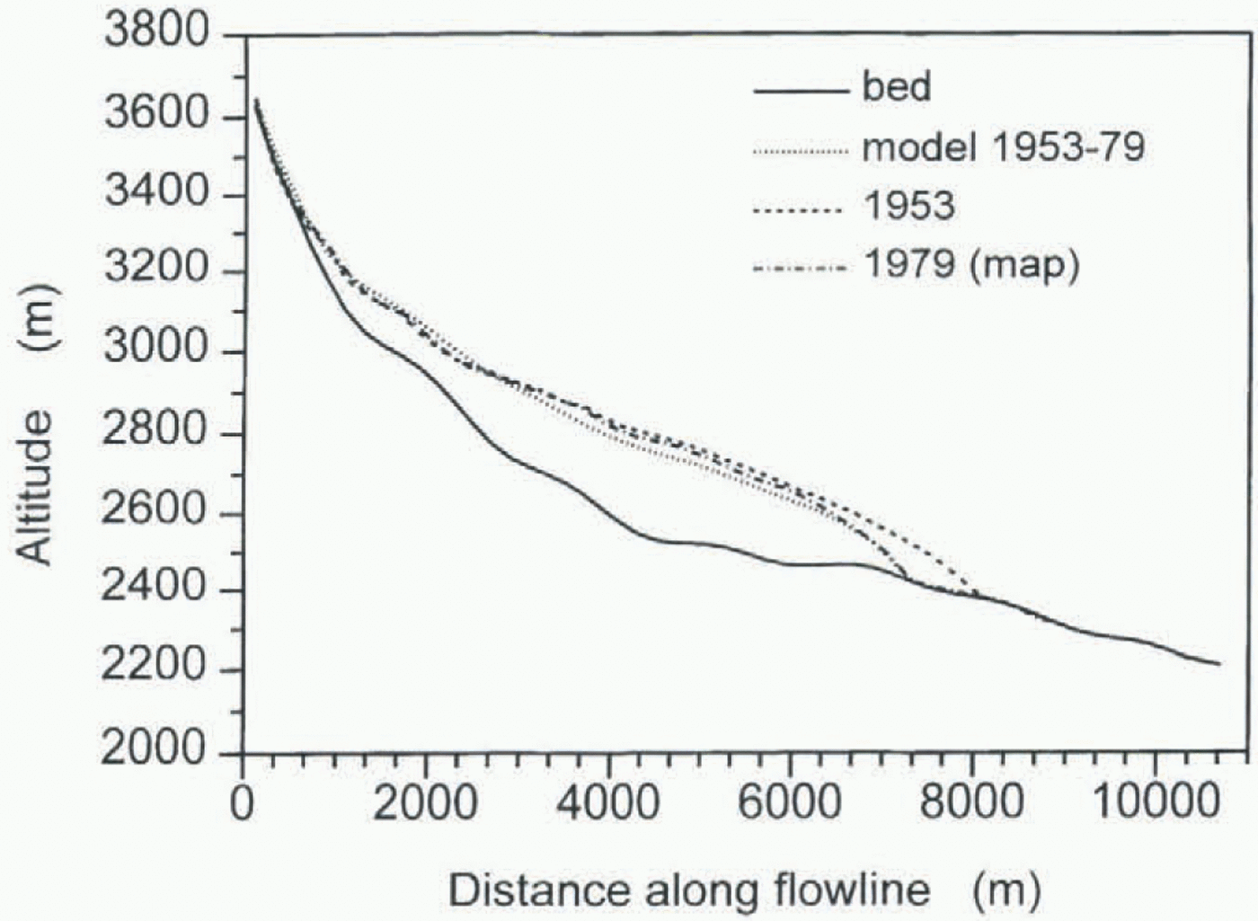
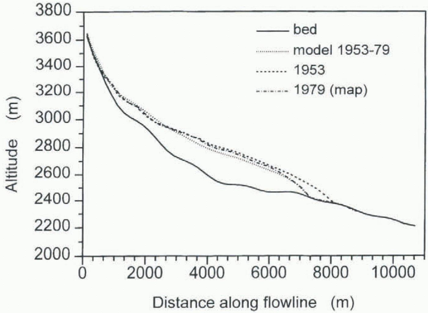
For all model runs the initial ice thickness profile was obtained from a map. The calculated profile of the last year of the simulation was then compared to the corresponding map profile. Additionally a comparison between calculated and observed front positions was made. In the calibration run (1953–79) f 1 and f 2 were varied until the result of the simulation was as close as possible to the map. Figure 6 shows the longitudinal ice thickness profiles of the 1953 and 1979 maps and the calculated end profile for 1979. For the calibration, emphasis was laid on the agreement of model and map profile in the tongue region, since differences in ice thickness in the upper part of the glacier are partly caused by strong simplification of the geometry. The resulting values for f 1 and f 2 are 1.7 x 10⁻²⁴ m6 s–1 N–3 and 1.3 x 10⁻¹⁷ m5 s–1 N–2, respectively.
Result (calculated ice thickness profile) of the simulation 1953–79 used to determine the parameters f1 and f2.
5 Reconstruction Back To Ad 1850
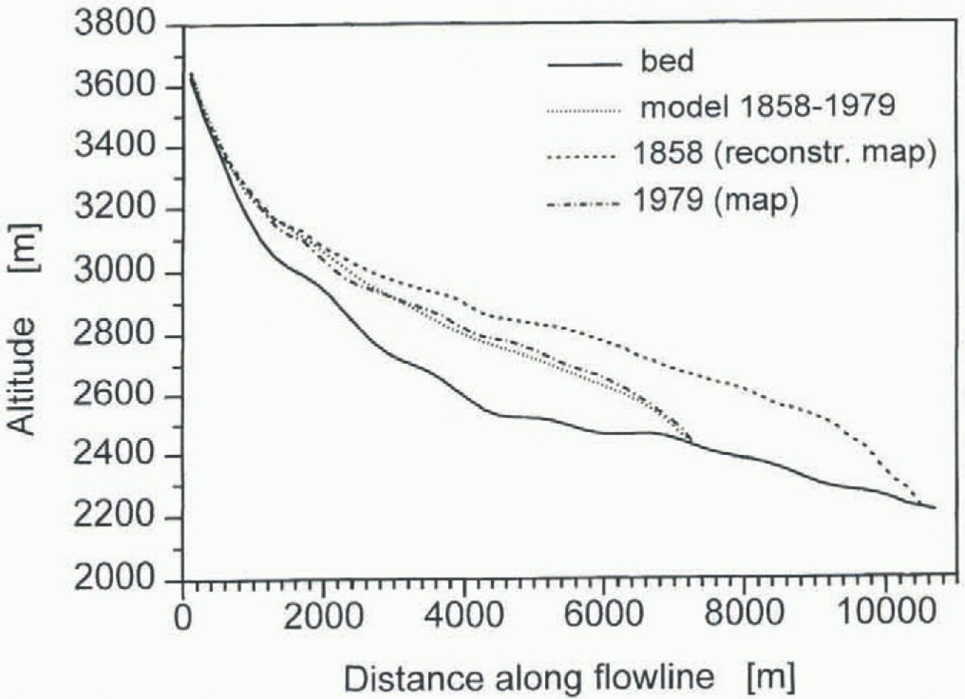
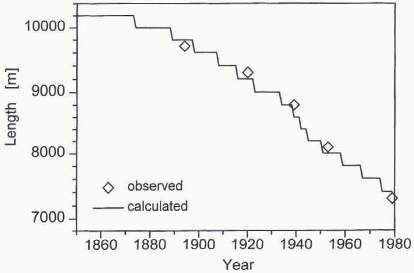
In figures 7 and 8 the results of the simulation 1858–1979 are shown. As forcing function the mass balance calculated from climate data (see Fig. 5) was used. The start year 1858 had to be chosen because precipitation of Marienberg was not measured before that year. Figure 7 shows the calculated
Result of the simulation 1858–1979: calculated longitudinal ice thickness profile in the end year 1979 compared to the map of the year 1979.

Result of the simulation 1858–1979: calculated and observed front positions.
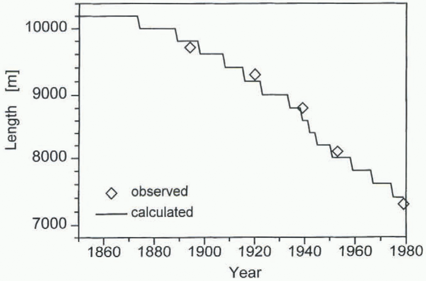
thickness profile for 1979 compared with the 1979 map profile. The profiles agree very well; slight differences are mostly due to the strongly simplified geometry, especially in the upper part of the glacier. In Figure 8 the front positions during the whole run are plotted. Within the accuracy of the model (200 m grid-point distance), calculated and observed front positions are equal. Also the fast retreat during the 1940s can be seen clearly.
The simulation with the dendro-mass balances as forcing (back to 1850) gives similar results.
6 Discussion And Conclusion
It is very encouraging and promising that, with such a relatively simple model, for the first time the reconstruction of historical variations of a glacier back to about AD 1850 using climate data was possible with satisfactory accuracy.
This reconstruction of a time period for which we have both the climate data and the glacier information needed to control the results is the basic requirement for any simulation further backwards (or for any future scenarios)! For the time before 1850 some difficulties arise, partly glacier-specific (tributaries, etc.), partly in principle (mass-balance parameterization, sliding). Thus the simulation is not yet successful prior to 1850.
Recently obtained radar ice-thickness data can help to improve the parameterization of the glacier geometry and, together with additional proxy data (new Alpine ice-core data, more historical documents), might increase the chances of a successful simulation of Hintereisferner back to AD 1600.
Acknowledgements
The work presented here is part of a Ph.D. thesis at the University of Innsbruck and was sponsored by the Austrian National Committee for the International Geosphere–Biosphere Project (IGBP).