1. INTRODUCTION
Let T be the lifetime of a reliability system of order n and X 1, X 2, … , X n the lifetimes of its components. If we assume that X 1, X 2, … , X n are independent and identically distributed (i.i.d.) according to a common underlying continuous distribution, the signature of the system is defined as the probability vector s(n) = (s 1(n), s 2(n), … , s n(n))′ with

where X (1) ≤ X (2) ≤ ··· ≤ X (n) are the order statistics of the sample X 1, X 2, … , X n. It can be verified that, in the i.i.d. case, the coordinates s i(n) of the signature depend only on the system structure, not on the (common) distribution of X i. As a matter of fact, n!s i can be calculated by examining the minimal cut sets of the system and counting how many among the n! equally likely permutations of X 1, X 2, … , X n result in a minimal cut set failing upon the occurrence of X (i).
The signature of a system is closely related to many well-known reliability concepts, a fact turning it into a very important tool for investigating the performance of a coherent structure and comparing structures with each other. For example, the reliability polynomial of a structure can be easily expressed in terms of the signature; the stochastic ordering for systems' lifetimes is often made feasible by simply comparing their signatures and so forth. For a detailed and up-to-date presentation of the signature of coherent systems and their applications, the interested reader is referred to the excellent publication of Boland and Samaniego [Reference Boland, Samaniego, Soyer, Mazzuchi and Singpurwalla1].
A linear (circular) consecutive k-out-of-n: F system consists of n components that are linearly (circularly) arranged and the system fails if and only if at least k consecutive components fail. The most popular applications of these systems, which were first introduced by Kontoleon [Reference Kontoleon12], pertain to telecommunication and pipeline network modeling, as well as integrated circuitry design. The term “consecutive k-out-of-n: F system” was first coined by Chiang and Niu [Reference Chiang and Niu6], and since then, it has attracted considerable research interest (for a review, see Chao, Fu, and Koutras [Reference Chao, Fu and Koutras4], Chang, Cui, and Hwang [Reference Chang, Cui and Hwang3], or Kuo and Zuo [Reference Kuo and Zuo14]).
Derman, Liebermann, and Ross [Reference Derman, Lieberman and Ross9] raised the interesting question of whether the family of consecutive k-out-of-n: F systems preserves the increasing failure rate (IFR) property (i.e., whether the system's lifetime is IFR when its components have statistically i.i.d. IFR lifetimes). This question was answered in the negative for the general case; however, it initiated a remarkable research interest for a detailed investigation of the range of k and n values that guarantee the IFR preservation or the opposite. Hwang and Yao [Reference Hwang and Yao10] treated in detail the special cases k = 2 and k = 3 and showed that, with a handful of exceptions, the IFR property is not preserved, Cui, Hawkes, and Jalali [Reference Cui, Hawkes and Jalali8] proved that for each k ≥ 2, there exists an n k such that the system does not preserve the IFR property for all n ≥ n k, whereas Cui [Reference Cui7] provided an upper bound for n k.
Samaniego [Reference Samaniego15] offered a complete characterization of the class of coherent systems that have the above property (i.e., are closed under i.i.d. IFR components) by exploiting the notion of signature. More specifically, he proved the following necessary and sufficient condition for a system's lifetime to be IFR whenever its component lifetimes X 1, X 2, … , X n are i.i.d. and follow an IFR distribution: The function
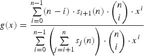
must be increasing for x > 0. Therefore, should one be able to compute the signature of a system, a positive or negative answer could be offered to the question of whether the IFR property is preserved for it.
Motivated by the aforementioned discussion, we present some tools that facilitate the calculation of the signature of a system and a simple sufficient condition for proving the nonpreservation of the IFR property (Section 2). In Section 3 we establish a recurrence relation for the computation of the signature of a linear consecutive k-out-of-n: F system and provide a formula that expresses the signature of a circular consecutive k-out-of-n: F system in terms of the signature of the linear one. Finally, in Section 4 we use the notion of signature to establish several results on the IFR preservation property of consecutive k-out-of-n: F systems, and in Section 5 we illustrate how one can take advantage of the outcomes of the previous sections to proceed to the stochastic comparison of the reliability structures' lifetimes.
2. GENERAL RESULTS
Let X 1, X 2, … , X n denote the component lifetimes of a reliability structure with n components and T denote the system's lifetime. Throughout this work we assume that the lifetimes X i are i.i.d. and, therefore, the probability that the system fails upon the ith component failure does not depend on the underlying continuous distribution of X i. Then the signature of the system is defined as the probability vector (s 1(n), s 2(n), … , s n(n)), with

where X (1) ≤ X (2) ≤ ··· ≤ X (n) are the order statistics of a random sample drawn from an arbitrary continuous lifetime distribution. In words, s i(n) is the proportion of permutations, among the n! equally likely permutations of X 1, X 2, … , X n, that result in a minimal cut set failing upon the occurrence of X (i).
Let us next denote by r i(n) the number of path sets of the structure with exactly i working components. Then s i(n) is related to the quantities

through the system of equations

or, equivalently,

(convention : a 0(n) = 0).
The next proposition, which will prove useful in the sequel, establishes a relation between the double generating function of r i(n),
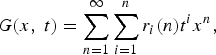
and the double generating function of the quantities
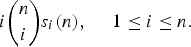
Proposition 2.1
The double generating function of 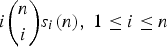 , is given by

where

Proof
Substituting expression (2.1) on the right-hand side of (2.2), we can readily deduce

Therefore,
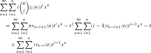
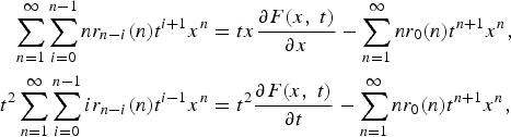
and the result we are looking for is effortlessly established on noting that the three terms on the right-hand side take on the forms
and

respectively.■
In view of Proposition 2.1, should one achieve to express F(x, t) = G(xt,1/t) as a rational function of x and t, one can then establish a recurrence for  , therefore obtaining a recurrence for s i(n). In the next section, we will exploit this approach for the linear consecutive k-out-of-n: F system.
As already mentioned in the Section 1, once the signature of a structure has been computed, one can use Samaniego's [Reference Samaniego15] condition (1.1) to determine whether the structure preserves the IFR property. In Proposition 2.2 we will provide a simple condition that can guarantee the nonpreservation of the IFR property for a reliability system. This condition requires the evaluation of only two of the n coordinates of the signature vector.
The proof of Proposition 2.2 will be couched on the following simple result, pertaining to the monotonicity of a rational function.
Lemma 2.1
Let

be a rational function of x with αm ≠ 0, βm ≠ 0. If

then there exists a positive x 0such that h(x) is strictly decreasing for x > x 0.
Proof
It is immediate that the function f(x) = h(1/x) can be expressed as

and its first derivative may yield the form

Since

we conclude that there exists an ɛ > 0 such that f′(x) > 0 for 0 < x < ɛ. Therefore, f will be strictly increasing for 0 < x < ɛ, which, in turn, guarantees that h(x) = f(1/x) will be decreasing for x > (1/ɛ) = x 0.■
Proposition 2.2
Let n 0 (1 ≤ n 0 < n) be the minimum number of working components in a reliability structure such that the system can still operate successfully. If

for i 0 = n − n 0, then the system does not preserve the IFR property.
Proof
By the definition of n 0, the probability that the ith component failure is fatal for the system's operation vanishes for all n − n 0 + 2 ≤ i ≤ n [i.e., the last nonvanishing coordinate of the signature (probability) vector (s 1(n), s 2(n), … , s n(n)) is s n−n 0 + 1(n)]. It is now clear that the function g(x) is a rational function of x with a common degree of the numerator and denominator, namely

and one can appeal to Lemma 2.1 to establish a sufficient condition for the IFR property not to be preserved. A direct comparison of (2.2) and (2.1) reveals that

and since

the proof is complete.■
It is worth mentioning that the special case n 0 = n that was excluded from Proposition 2.2 (because i 0 = 0 and s 0(n) is meaningless) corresponds to a parallel system; it is well known that such a structure does not preserve the IFR property.
As an illustration of how Proposition 2.2 could be applied, let us consider the case of a consecutive k-out-of-n: F system with k = 2, n = 3. Writing down all possible 3! orderings of the component lifetimes X 1, X 2, X 3, we can easily identify the signature vector

Since n 0 = 1, i 0 = 2, and

we conclude that the system does not preserve the IFR property.
3. RECURRENCE RELATION FOR THE SIGNATURE OF A CONSECUTIVE k-OUT-OF-n: F SYSTEM
Let us first consider a linear consecutive k-out-of-n: F system. Then a typical path set of size i will result if we arrange the i working components in a line, therefore creating i + 1 spacings-urns (i − 1 urns between the i successive working components, one before the first and one after the last one) and then distribute the remaining n − i failed components so that no urn contains k or more components. As a consequence, if we denote by M(r, m) the number of ways of distributing r like objects into m distinct urns so that each urn contains at most k − 1 components, it is apparent that the number of path sets of the system with i working components can be expressed as

It is worth mentioning that the above quantity coincides with the numbers N(i, n − i + 1; k − 1) exploited by Derman et al. [Reference Derman, Lieberman and Ross9] to study the reliability of a consecutive k-out-of-n: F system. We are now ready to prove the next proposition.
Proposition 3.1
Let s i(n), i = 1, 2, … , n, be the signature of a consecutive k-out-of-n: F system.
(a) The double generating function of
 is given by (3.2)
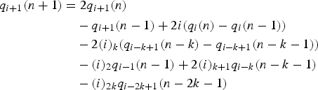
(b) The quantities q i(n) = (n)is i(n), i = 1, 2, … , n, satisfy the following recurrence relation:
(3.3)for i = 0, 1, … , n − 1 and n ≥ 2k + 2.
 is given by

Proof
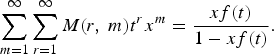
(a) The generating function of the number M(r, m), r = 1, 2, … , of distributions of r indistinguishable objects into m distinguishable urns, each of limited capacity k − 1, equals
whereis the enumerator of each individual urn (see, e.g., Charalambides [Reference Charalambides5, Chapt. 9]). Multiplying by x m and summing up for all m = 1, 2, … , we get(3.4)By virtue of (3.1), the quantity F(x, t) given in (2.4) can be written aswhich, on using the transformation n − i + 1 = m in the inner summation, takes on the formRecalling (3.4), we obtainand the right-hand side of (3.2) is readily deduced by calculating the partial derivatives of F(x, t) and replacing them in (2.3). We mention that the above expression F(x, t) could also be derived as a special case of a more general result of Koutras and Papastavridis [Reference Koutras and Papastavridis13]; however, we chose to include a short proof so that the manuscript becomes self-contained.(b) If we introduce the notation
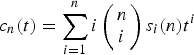
(3.5)and write (3.2) in the form(3.6)we can easily verify (by noting that the coefficients of x n+1 of the left-hand side should vanish for n ≥ 2k + 1), the following recursive scheme for c n(t) is obtained:We next substitute c n(t) by (3.5) in the last equality and pick out the coefficients of t i+1, i = 0, 1, … , n − 1, on both sides; the recurrence relation ensues by straightforward algebraic maneuvering. ■






In order to launch the recursive scheme (3.3), a number of initial conditions is necessary. These conditions can be effortlessly derived by exploiting again (3.6), now taking into account the coefficients of x n+1, n < 2k + 1. A sufficient set of initial conditions that permit the computation of q i(n) (and, therefore, s i(n)) is provided by

The additional values q i(n), k + 1 < n ≤ 2k + 2, needed before we start using (3.3) can be obtained by exploiting the same scheme and setting q i(n) = 0 if i ≤ 0, n ≤ 0, i < k, or n < k and in the event of deriving any negative value of q i(n).
It is noteworthy that after some straightforward algebraic manipulations on the right-hand side of (3.2), the following alternative form can be gained for the double generating function of  :
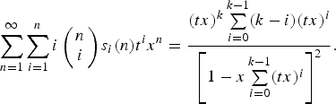
Exploiting this expression, one could derive a new recurrence relation for s i(n) by following exactly the same steps that were used in the proof of Proposition 3.1. Since this recurrence will express s i(n) in terms of all s i−j(n − r), j = 0, 1, … , 2k − 2, i = 1, 2, … , 2k, and is much more intricate than (3.3), we are not pursuing this approach further.
As already mentioned in Section 1, the quantity

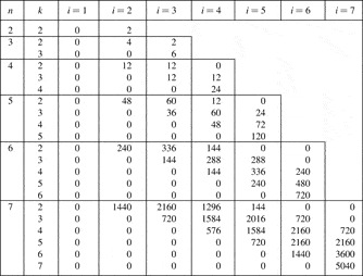
is always an integer; in fact, s¯i(n) counts how many among the n! equally likely permutations of component lifetimes X 1, X 2, … , X n result in a minimal cut set failing upon the occurrence of X (i). Therefore, it might be of interest to first compute the sequence of integers s¯i(n), 1 ≤ i ≤ n, and then proceed to the calculation of s i(n).
It is not difficult to verify that s¯i(n), 1 ≤ i ≤ n, obey the following recurrence relation:

for i = 0, 1, … , n − 1 and n ≥ 2k + 2 with initial conditions

The additional values s¯i(n), k + 1 < n ≤ 2k + 2, can be obtained by exploiting the same scheme and setting s¯i(n) = 0 if i ≤ 0, n ≤ 0, i < k, or n < k or in the event of deriving a negative value of s¯i(n).
Table 3.1 gives the quantities s¯i(n) for consecutive k-out-of-n: F systems for 2 ≤ k ≤ n and n = 2, 3, … , 7.
Quantities s¯i(n) for Consecutive k-out-of-n: F Systems

The computation of the signature of a circular consecutive k-out-of-n: F system can be easily carried out with the aid of the following result.
Proposition 3.2
If s iC(n) and s i(n), 1 ≤ i ≤ n, are the signatures of a circular and a linear consecutive k-out-of-n: F system, respectively, then

Proof
Applying the general identity (2.5) for a linear consecutive k-out-of-(n − 1): F system and a circular consecutive k-out-of-n: F system, we can write


where r i(n) = M(n − i, i + 1) are as in the earlier analysis and r iC(n) = M C(n − i, i + 1) refer to the case where the first and the last components of the system are considered as neighboring components. In the latter case, M C(r, m) coincides with the number of ways of distributing r indistinguishable objects into m distinct urns 1, 2, … , m, so that each of the urns 2, 3, … , m − 1 contains at most k − 1 components and urns 1 and m contain, in total, at most k − 1 components as well. As Koutras and Papastavridis [Reference Koutras and Papastavridis13] proved, M C(r, m) can be expressed through M(r, m − 1) as follows:

In view of this equality, we obtain

Now, we substitute twice this result on the right-hand side of (3.9) to deduce the expression

and making use of (3.8), the following equality ensues:

This completes the proof.■
4. THE IFR PRESERVATION PROPERTY OF A CONSECUTIVE k-OUT-OF-n: F SYSTEM
As already mentioned in Section 1, Derman et al. [Reference Derman, Lieberman and Ross9] were the first to raise the interesting question of whether the family of consecutive k-out-of-n: F systems preserves the IFR property. Quite a few publications appeared on this subject in the following years; see, for example, Hwang and Yao [Reference Hwang and Yao10], Cui et al. [Reference Cui, Hawkes and Jalali8], and Cui [Reference Cui7].
As an application of the results presented in the previous sections, we will proceed to the investigation of the IFR preservation property for the family of consecutive 2-out-of-n: F systems. The double generating function (3.7) now reads

and writing the right-hand side in the form of a double power series and fetching the coefficients of t ix n, we conclude that

which yields

If n is even, the parameters used in Proposition 2.2 are

and one can easily check that

Manifestly, the right-hand side is greater than n 0 for n 0 > 5 and, therefore,

which, in lieu of Proposition 2.2, yields that the consecutive 2-out-of-n: F system does not preserve the IFR property for all even n ≥ 10.
If n is odd, then

and proceeding in a similar manner, we obtain

which, in turn, guarantees that the consecutive 2-out-of-n: F system does not preserve the IFR property for all odd n ≥ 3.
The earlier arguments leaves unidentified the cases n = 2, 4, 6, 8, which, however, can be readily treated with the aid of Samaniego's [Reference Samaniego15] necessary and sufficient condition (1.1). By way of example, we mention that for n = 4, we deduce (see, e.g., Table 3.1)

which is increasing in x; as a consequence, the consecutive 2-out-of-4: F system preserves the IFR property. The same conclusion can be drawn by a similar procedure for the other three missing cases (i.e., for n = 2, 6, 8).
The above results seem to have been proven for the first time by Hwang and Yao [Reference Hwang and Yao10]. To accomplish that, they initially stated a sufficient condition for the IFR property not to be preserved, couched on the numbers M(r, m) (see Section 3). As a matter of fact, it can be easily shown that condition (2.6) reduces to Hwang and Yao's condition in the special case of consecutive k-out-of-n: F systems.
Hwang and Yao [Reference Hwang and Yao10] and Cui et al. [Reference Cui, Hawkes and Jalali8] treated the cases k = 3 and k = 5, 6 as well. Their results can also be established by employing similar arguments as for the case k = 2 earlier; however, the details are too technical and are left as an exercise for the interested reader.
5. STOCHASTIC COMPARISON OF RELIABILITY STRUCTURES
There are several ways to compare two coherent systems of a given size. In this section we will illustrate how computation of signatures can lead to the foundation of stochastic relationships between systems. The concept of stochastic order is a useful tool in comparing systems' lifetimes and one can easily find in the literature a variety of stochastic orderings. Throughout this work, we focus on the usual stochastic order, studied by Shaked and Shanthikumar [Reference Shaked and Shanthikumar16], which we will depict briefly in the following. Let us first denote by T 1 and T 2 the lifetimes of two systems with cumulative distribution functions F 1 and F 2, respectively. Then T 1 is said to be stochastically smaller than T 2 in the usual stochastic order (denoted by T 1 ≤stT 2) if the following inequality holds true:

Roughly speaking, T 1 ≤stT 2 if and only if T 1 is less likely than T 2 to take on values beyond t.
Kochar, Mukerjee, and Samaniego [Reference Kochar, Mukerjee and Samaniego11] established a sufficient condition for the stochastic ordering of systems' lifetimes, which is based on their signatures. More specifically, they proved that if
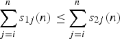
for all i = 1, … , n (s 1j(n), s 2j(n), j = 1, 2, … , n, are the signature coordinates of the two systems), then T 1 ≤stT 2.
As an illustration of how the results presented in the present article could be exploited for the stochastic comparison of reliability structures, let consider the family of k-out-of-n: F systems (which fail whenever at least k components fail) and the consecutive linear and circular k-out-of-n: F systems. For the signature s(n) = (s 1(n), s 2(n), … , s n(n))′ of the first class, we have (see, e.g., Boland and Samaniego [Reference Boland and Samaniego2])

the signatures of the consecutive linear and circular k-out-of-n: F systems can be easily computed by the aid of Propositions 3.1 and 3.2, respectively. Then condition (5.2) can be used to establish a stochastic ordering between systems' lifetimes.
Table 5.1 presents the stochastic ordering that can be achieved among all of the families of systems mentioned earlier, for n = 5 and all k = 1, 2, … 5. Needless to say k = 1 corresponds to a series system and k = 5 corresponds to a parallel one.
Stochastic Ordering Among Systems of Order n = 5

Looking at Table 5.1, it is easily verified that the 11 coherent systems can almost totally be ordered. More specifically, we were able to shed light on the 52 pairs out of the 55 possible pairwise comparisons among these systems of order 5. It should be stressed that the remaining three pairs cannot be ordered, as can be easily substantiated by considering their reliability functions in the simplest case where all components have exponential lifetimes.
Some of the comparisons depicted in Table 5.1 can be effortlessly established by alternative approaches (e.g., by examining whether the respective families of minimal cut sets can be ordered). This is feasible, e.g., when comparing systems with the same k: the k-out-of-n: F system has a larger family of minimal cut sets than the circular consecutive k-out-of-n: F system and the latter has a larger family of minimal cut sets than the linear consecutive k-out-of-n: F system.
However, there are quite a few pairs of systems for which the families of minimal cut sets cannot be ordered. Such a case arises when comparing the 2-out-of-5: F system (which has  minimal cut sets of the form {i, j}, with 1 ≤ i < j ≤ 5) to the linear 3-out-of-5: F system (which has three minimal cut sets of the form {i, i + 1, i + 2}, i =1, 2, 3). In this case, their signatures can be easily computed as

respectively, and resorting to (5.2), we can conclude that the first system's lifetime is stochastically smaller than the lifetime of the second one.
Acknowledgment
Research was supported by the program Pythagoras, EPEAEK II, Ministry of National Education and Religious Affairs, cofinanced by the European Social Fund.