1. Introduction
A study of a liquid film flowing over a thin fibre finds applications in a variety of industrial applications such as lubrication of rotors and stators (Bhushan Reference Bhushan2020), dripping of water during desalination (Sadeghpour Reference Sadeghpour2020), liquid film based thermal cooling (Bar-Cohen, Arik & Ohadi Reference Bar-Cohen, Arik and Ohadi2006) and in the preparation of functional coatings over fibres (Rivero et al. Reference Rivero, Urrutia, Goicoechea and Arregui2015). In the low flow rate regime, Goren (Reference Goren1962) and Solorio & Sen (Reference Solorio and Sen1987), motivated by the droplet patterns on a spider’s web, performed linear instability of an annular thread of liquid and showed that the film is unstable and breaks up into droplets. In flowing films, spontaneous breakup of the liquid film that travel downstream was experimentally observed by Quéré (Reference Quéré1999) during drawing of fibres through liquids.
Kliakhandler, Davis & Bankoff (Reference Kliakhandler, Davis and Bankoff2001) considered very viscous fluid films flowing down a fibre and studied the characteristics of the waves forming at the film interface. They showed that the film flow exhibits three regimes based on the flow rate conditions, namely, the droplet merging (convective regime), Rayleigh–Plateau instability (chain of droplets) and isolated droplet formation regimes. Ruyer-Quil et al. (Reference Ruyer-Quil, Treveleyan, Giorgiutti-Dauphiné, Duprat and Kalliadasis2008) performed experiments on a film flowing down a cylindrical fibre and reported three different regimes based on the inlet flow rate, namely, drop-like, wave-like and an intermediate regime. Flow regimes are essentially dominated by Rayleigh–Plateau instability (drop-like) at low flow rates, and Kapitza instability (wave-like) for thicker films in the inertial regime. A fore–aft symmetry is observed in the drop-like regime, whereas in the wave-like regime the leading end of the droplet has a steeper slope compared with the trailing end. Influence of the control parameters, such as fluid properties, flow rate, inlet perturbations and nozzle to fibre diameter ratio, on the dynamics of film flow has been studied in the last few decades.
Sisoev et al. (Reference Sisoev, Craster, Matar and Gerasimov2006) discovered that attracting wave regimes and dominant waves in fibre flow are influenced by the system parameters and forcing conditions. Inlet perturbations and their impact on flow behaviour have been further examined by Duprat, Ruyer-Quil & Giorgiutti-Dauphiné (Reference Duprat, Ruyer-Quil and Giorgiutti-Dauphiné2009). They observed that the speed of the travelling waves decreases with a decrease in the forcing frequency, which is estimated from the average slope of the crest lines on the spatio-temporal diagram. Forcing amplitude also has an influence on the other characteristics of the travelling waves. The healing length, defined as the length downstream of the nozzle over which the instability grows, decreases with an increase in the amplitude, and the coalescence events near the nozzle that result in bigger droplets increase with an increase in the perturbation amplitude. Thus, healing length can be defined as the length of the flow below the nozzle up to the emergence of the first droplet, as also discussed in Ji et al. (Reference Ji, Sadeghpour, Ju and Bertozzi2020).
Using the mathematical formulation of Ya (Reference Ya1967), Shkadov & Sisoev (Reference Shkadov and Sisoev2004) proposed a model for the nonlinear gravity–capillary waves with a single parameter based on a scaled Reynolds number. They showed that, with an increase in the Reynolds number, the number of travelling wave solutions increases. Trifonov (Reference Trifonov1992) proposed an alternative approximate two-equation model (for film thickness and volumetric flow rate), derived in the long-wave approximation using an integral balance with an assumed velocity profile containing parabolic and logarithmic terms, that yields steady travelling wave solutions. Non-uniqueness of these solutions suggests the existence of many more families of solutions. Using Trifonov’s two-equation model, Sisoev et al. (Reference Sisoev, Craster, Matar and Gerasimov2006) performed numerical simulations in the nonlinear regime and investigated the selection mechanisms for the dominant waves observed in experiments. In addition, they showed the existence of several other naturally excited waves and forced wave solutions that are usually not observed in experiments. Thin film equations using the lubrication equation and curvature effects were derived by Frenkel (Reference Frenkel1992). Using Frenkel’s formulation, Kalliadasis & Chang (Reference Kalliadasis and Chang1994) could capture the experimental observations of Quéré (Reference Quéré1999) showing the formation of axisymmetric travelling droplets. Further, Roy, Roberts & Simpson (Reference Roy, Roberts and Simpson2002) accounted for the azimuthal and in-plane curvature terms in the Frenkel equation and extended them to higher-order terms in the long-wave parameter (thickness of the film to the radius of the fibre). Ruyer-Quil et al. (Reference Ruyer-Quil, Treveleyan, Giorgiutti-Dauphiné, Duprat and Kalliadasis2008) (also see Roberts & Li Reference Roberts and Li2006) presented a two-equation model (thickness and flux) to capture the dynamics of a film flowing down a fibre. Some interesting features of the instability were captured in their simulations, including the role of the Kapitza instability mode and the travelling wave branches of the solutions. Both absolutely unstable regimes and the convectively unstable regimes observed in Duprat et al. (Reference Duprat, Ruyer-Quil, Kalliadasis and Giorgiutti-Dauphiné2007) were captured. Recently, Ji et al. (Reference Ji, Sadeghpour, Ju and Bertozzi2020) performed numerical simulations by solving the weighted residual boundary layer equations proposed in Ruyer-Quil et al. (Reference Ruyer-Quil, Treveleyan, Giorgiutti-Dauphiné, Duprat and Kalliadasis2008) and showed an excellent agreement with the experiments.
Although the essential features of the instability modes have been captured in the previous experimental, theoretical and numerical studies such as the Rayleigh–Plateau instability (Kliakhandler et al. Reference Kliakhandler, Davis and Bankoff2001; Duprat et al. Reference Duprat, Ruyer-Quil, Kalliadasis and Giorgiutti-Dauphiné2007), droplet merging (convective regime Duprat et al. Reference Duprat, Ruyer-Quil and Giorgiutti-Dauphiné2009) and attracting wave regimes (Sisoev et al. Reference Sisoev, Craster, Matar and Gerasimov2006), the effect of the inlet conditions at the nozzle has gained interest only recently. Duprat et al. (Reference Duprat, Ruyer-Quil and Giorgiutti-Dauphiné2009) explored the effect of temporal perturbations in the inlet flow at the nozzle on the instability mode selection. When the nozzle-to-fibre diameter ratio is large (Ji et al. Reference Ji, Sadeghpour, Ju and Bertozzi2020; Sadeghpour Reference Sadeghpour2020), the convective regime transitions to the Rayleigh–Plateau regime. Duprat et al. (Reference Duprat, Ruyer-Quil and Giorgiutti-Dauphiné2009) also showed that, with an increase in the nozzle diameter, the healing length decreases and the droplet spacing increases. Modelling approaches that include intermolecular forces for the thin film dynamics and domain transformation techniques for numerical simulations improve the agreement with the experimental results (Ji et al. Reference Ji, Sadeghpour, Ju and Bertozzi2020; Liu & Ding Reference Liu and Ding2021). These studies collectively provide a comprehensive understanding of film flow down a fibre, shedding light on the emergence of wave regimes, dominant wave selection and the influence of system parameters and forcing conditions. However, the role of the fibre geometry on the film evolution has been scantly studied. The study of liquid films flowing over structured surfaces has implications in several industries, specifically for applications such as coating, desalination and particle collection (Dietze Reference Dietze2019; Sadeghpour Reference Sadeghpour2020; Xie et al. Reference Xie, Liu, Wang and Chen2021). Granular chains with functional coatings find applications in granular conductors (Xu, Qin & Heath Reference Xu, Qin and Heath2009), flexible electronics (Su et al. Reference Su, Li, Chen, Huang, Qin, Li, Zhang and Song2016) and also as impact protectors (Machado & Sen Reference Machado and Sen2021). Granular chains have also been used for making artificial cilia in robotic applications (Breidenich et al. Reference Breidenich, Wei, Clatterbaugh, Benkoski, Keng and Pyun2012).
Previous research has shown that the roughness of the fibres (Sadeghpour Reference Sadeghpour2020), the geometric shapes (Xie et al. Reference Xie, Liu, Wang and Chen2021) and the corrugations of the walls (Dietze Reference Dietze2019) significantly affects the droplet dynamics and enhances interfacial transport. The present study systematically investigates the effect of discrete geometrical perturbations, modelled by beads on a fibre, to gain insights that can guide the design of fibre-based devices with controlled instability and thus enhanced performance.
Recent studies related to fibre geometries like elliptical (Li, Carvalho & Kumar Reference Li, Carvalho and Kumar2017) and conical fibres (Chan et al. Reference Chan, Lee, Pedersen, Dalnoki-Veress and Carlson2021; Xie et al. Reference Xie, Liu, Wang and Chen2021) show that the mode of instability is significantly affected by the fibre’s geometry. In particular, the conical fibre has been shown to have a significant effect on the droplet formation and the size distribution. We perform experiments as well as simulations for flow over a fibre with a single spherical bead. Further, we discuss the features of the instability for flow over a granular chain of spherical beads on the fibre. Finally, we compare the variations introduced in the liquid film morphology due to the presence of a rigid bead with those when the inlet velocity is perturbed.
(a) The experimental set-up used for high-speed imaging. The fibre is stretched and both the ends are clamped. The inset marked as ‘i’ shows the nozzle geometry with the fibre passing through the centre. A syringe pump is employed for generating a given flow rate. A diffuser plate in front of an LED lamp is employed for backlighting and a Photron camera, Nova S9, is used for high-speed imaging. (b–d) Configurations of the coaxial nozzle with the fibre used to examine the influence of bead placement: (b) no bead, (c) bead near the nozzle, (d) bead far from the nozzle.

2. Experimental set-up
Figure 1(a) shows a schematic of the high-speed imaging set-up used for studying the dynamics of a film flowing down on a fibre. The various components of the experimental set-up are labelled in the schematic diagram. The main test rig consists of a syringe pump (New Era Pump Systems, NE-1000), a syringe and a hypodermic needle, assembly of a vertical fibre and a tank collecting the dispensed liquid. Shadowgraphy module for visualising the fluid film evolution using a high-speed camera (Photron Fastcam Nova SA9) is connected through a computer (i7 processor) to an image acquisition software. A diffuser plate is used in front of an LED source. Panels (b–d) show 3 different fibre configurations: a flat fibre (b), a fibre with a bead placed close to the nozzle (c) and one with a bead located far downstream from the nozzle (d). In the present experimental study, we use silicone oil with density,
 $\rho = 960$
kg m−
 $^3$
, viscosity
 $\mu = 48$
mPa S and surface tension coefficient
 $\gamma = 20.6$
mN m−1. We use two nozzles with a ratio of nozzle to fibre diameter,
 $\alpha =D_n/D_f$
, of
 $4.7$
and
 $14.28$
.
The flow rate was imposed using a New Era NE-4000 syringe pump with a specified accuracy of
 $1 \, \%$
and a minimum resolution of 1.459
 $ \mu \textrm{l/hr}$
, ensuring repeatable flow conditions. Beads were manually positioned using a calibrated micrometre slide with
 $\pm$
0.1 mm accuracy, ensuring precise placement at fixed axial distances of 9.3 and 27 mm from the nozzle in our numerical simulations.
The key parameters that govern the physics of the above system are the density and viscosity of the liquid, surface tension of the liquid–air interface, the nozzle size
 $D_n$
, fibre diameter
 $D_f$
, flow rate
 $Q$
and the gravitational acceleration
 $g$
. The capillary length scale
 $l_c= \sqrt {(\sigma /(\rho g))}$
and the viscous length scale
 $l_{\nu } = \nu ^{2/3} g^{-1/2}$
(
 $\nu$
is the viscosity) are obtained by a balance between the gravitational and viscous forces. Based on the above parameters, the film dynamics can be described by four non-dimensional parameters, namely, the Kapitza number
 $\Gamma = \sigma /(\rho \nu ^{4/3} g^{1/3}) = (l_c/l_{\nu })^2$
(
 $\sigma$
is the surface tention coefficient), Reynolds number
 $Re = \rho Q/\mu \pi R_n$
, Bond number
 $Bo=\rho g R_n^2/\sigma$
and the ratio of nozzle to fibre diameters,
 $\alpha =D_n/D_f$
. We note that Duprat et al. (Reference Duprat, Ruyer-Quil and Giorgiutti-Dauphiné2009) used the Nusselt film thickness,
 $h_N$
, as the characteristic length scale, in contrast to the nozzle radius,
 $R_n$
, used here.
In order to get an estimate of the relative magnitude of capillary, inertial and viscous forces, we compute the Bond number
 $Bo = \rho g h_N^2/\sigma$
and Reynolds number
 $Re = (g h_N^3) / (\nu ^2)$
, where
 $h_N$
is the Nusselt film thickness.
We would like to note here that, although the inlet condition for the fluid film is
 $D_n - D_f$
, the film evolves downstream and theoretically should result in the equilibrium solution corresponding to a uniform thickness the Nusselt film thickness
 $ \bar {h}_N$
, as described in Craster & Matar (Reference Craster and Matar2006) and Ruyer-Quil et al. (Reference Ruyer-Quil, Treveleyan, Giorgiutti-Dauphiné, Duprat and Kalliadasis2008). This thickness is calculated from a steady-state balance of gravitational and viscous forces, given by
 \begin{align} Q = \frac {g \bar {h}_N^3 \, \phi \left(\bar {h}_N / R\right)}{\nu }, \end{align}
where
 $ Q$
is the volumetric flow rate,
 $ g$
is the gravitational acceleration,
 $ \nu$
is the kinematic viscosity and
 $ R$
is the fibre radius. The function
 $ \phi$
captures the correction for curvature (Ruyer-Quil et al. Reference Ruyer-Quil, Treveleyan, Giorgiutti-Dauphiné, Duprat and Kalliadasis2008). Based on Nusselt film height
 $\bar {h}_N \approx 0.512\,\text{mm}$
, which is comparable to the experimentally observed minimum film thickness. However, this equilibrium solution is unstable and results in formation of droplets separated by a thin fluid film between them.
Based on this value of
 $h_N$
, we get
 $Bo = 0.12$
and
 $Re = 0.91$
, indicating that surface tension forces do not have a significant effect on the flow dynamics. Heining, Wierschem & Aksel (Reference Heining, Wierschem and Aksel2007) studied the effect of capillary forces in such flows and concluded a strong surface tension can indeed modify the primary instability. However, for the current system, we note that the instability is essentially driven by inertial, gravitational and viscous forces. However, for low
 $Re$
, we note that the primary instability will be essentially Rayleigh–Plateau, as discussed in Ruyer-Quil & Kalliadasis (Reference Ruyer-Quil and Kalliadasis2012), with the droplets so formed convected with the flow.
3. Numerical formulation
Reduced-order models based on the long-wave approximation have been successfully used previously to describe thin film flows over smooth (Ruyer-Quil et al. Reference Ruyer-Quil, Treveleyan, Giorgiutti-Dauphiné, Duprat and Kalliadasis2008; Duprat et al. Reference Duprat, Ruyer-Quil and Giorgiutti-Dauphiné2009) or inclined corrugated surfaces (Trifonov Reference Trifonov2017; also see: Dietze Reference Dietze2019). For the case of a flat fibre (i.e. Blockage ratio, BR = 0), we have implemented and validated the Weighted-Residual Integral Boundary-Layer (WRIBL) model for the flat fibre case against our experimental results. The comparison is shown in figure 2. Trifonov (Reference Trifonov1998, Reference Trifonov2007) have studied the effect of periodic corrugations on a flat surface on the stability of the film. There have been several studies on the stability analysis using the long-wave approximation employed to model the sinusoidal corrugations at the wall (see for example Wierschem & Aksel Reference Wierschem and Aksel2003; Dávalos-Orozco Reference Dávalos-Orozco2007). Trifonov (Reference Trifonov2007) derived a nonlinear evolution equation for flow over a corrugated wall based on a small-wavenumber approximation and concluded that the waves at the interface can be mitigated for sinusoidal surface corrugations of a certain wavelength at the wall. In comparison with corrugations on a planar surface, theoretical studies on cylindrical fibres are few and far between. Film flow over a smooth cylindrical surface has been subjected to linear stability analysis of the base state solution corresponding to a uniform Nusselt film thickness (Ruyer-Quil et al. Reference Ruyer-Quil, Treveleyan, Giorgiutti-Dauphiné, Duprat and Kalliadasis2008; Duprat et al. Reference Duprat, Ruyer-Quil and Giorgiutti-Dauphiné2009). However, in the present study we look at the effect of bigger beads (
 $\textit{BR} \gt 0.5$
) where we expect a significant change in the initial unperturbed solution. We note that for such
 $\textit{BR}$
values the long-wave approximation is not valid and thus WRIBL cannot be employed to study these configurations. Introduction of a bead of size similar to the film thickness introduces a finite-amplitude perturbation. Solution corresponding to these finite-amplitude perturbations cannot be predicted using linear stability analysis. Nonlinear evolution equations, similar to the one derived by Dávalos-Orozco (Reference Dávalos-Orozco2007), can be employed. However, these equations can usually be derived only in the small-wavenumber (or large-wavenumber) limit. Recently, Trifonov (Reference Trifonov2007) (also see Dietze Reference Dietze2019; Bonart et al. Reference Bonart, Rajes, Jung and Repke2020) employed full Navier–Stokes simulations to study the nonlinear response of periodic surface corrugations on film flow over an flat inclined surface. Thus, we resort to full Navier–Stokes simulations in the present study.
Film thickness comparison between experiments and WRIBL model.

Here, we numerically study the dynamics of a Newtonian liquid film (density
 $\rho _l$
and viscosity
 $\mu _l$
) in quiescent air (density
 $\rho _a$
and viscosity
 $\mu _a$
) flowing down over a thin fibre from a nozzle. Schematics given in figures 3(a,b and c) show the various configurations that we investigate in this study. Figure 3(a) shows the configuration for a flat cylindrical fibre which has been studied earlier in Ji et al. (Reference Ji, Sadeghpour, Ju and Bertozzi2020) for different nozzle to fibre diameters,
 $D_n/D_f$
, where
 $D_n$
and
 $D_f$
are the nozzle and fibre diameters, respectively. The local thickness of the fluid film is denoted by
 $h(z,t)$
which is a function of the axial coordinate
 $z$
and time
 $t$
. Radial coordinate is denoted by
 $r$
and the origin is placed at the centre of the nozzle. Figure 3(b) shows the configuration we employ to study the effect of the presence of a corrugation on the fibre’s surface on the flow instability characteristics. The corrugation is modelled using an axisymmetric particle with radius of curvature
 $R$
and is placed at a distance
 $L_p$
from the nozzle. Figure 3(c) shows the geometry employed to study flow over a granular chain. The granular chain is made up of solid beads with a radius
 $R$
placed at a spacing of
 $\lambda _p$
on a thin cylindrical fibre.
Schematic showing fluid film of thickness,
 $h$
, flowing over a
 $(a)$
cylindrical fibre of diameter
 $D_{f}$
from a nozzle of diameter
 $D_{n}$
,
 $(b)$
a fibre with a rigid bead of radius,
 $R$
, located at
 $L_{p}$
from the nozzle’s exit and
 $(c)$
a fibre with torus granular chain with spacing between them
 $\lambda _{p}$
shown.
 $(d)$
Computational domain of length
 $L$
and width
 $W$
with the fibre placed at the axisymmetry boundary. A liquid film of thickness
 $h$
is injected into the computational domain from above. A coordinate frame (
 $r{-}z$
plane) is attached at the axis of symmetry with the
 $z$
-coordinate pointing in the direction of the gravitational acceleration (
 ${\boldsymbol{g}}$
). Ambient fluid is air (with density
 $\rho _{g} = 1\, {\rm kg}\, {\textrm m}^{-3}$
) and is assumed to be quiescent. Outflow boundary conditions are imposed at the bottom end.

We perform numerical simulations using the volume-of-fluid method in the two-phase flow open source code Gerris (Popinet Reference Popinet2003, Reference Popinet2009; Tomar et al. Reference Tomar, Fuster, Zaleski and Popinet2010). Computational domain chosen for the simulations is shown in figure 3(d). We perform axisymmetric simulations and thus only half of the domain, defined by length
 $L$
and width
 $W$
, as shown in the figure is employed for performing the simulations. The gravitational acceleration is in the
 $z$
direction (downward) and the ambient fluid is air. The computational domain is initialised with a flat film of liquid of uniform thickness (
 $D_n - D_f$
). Different geometries shown in the schematics in figures 3(a), 3(b) and 3(c) are generated using the following functions. For the flat cylindrical fibre
 \begin{equation} f(z) = R_f, \end{equation}
where
 $R_f$
is the radius of the fibre. For the configuration in figure 3(b), the following functional form is used to define the fibre and the corrugation:
 \begin{equation} f(x)= \begin{cases} R_f+\left[R^2-(z-L_p)^2\right]^{1/2} ,& \text{if } z-R \leqslant z\leqslant z+R \\[2pt] R_f, & \text{otherwise.} \end{cases} \end{equation}
A granular chain geometry (figure 3
c) can be similarly created by introducing a spatial periodicity in the above function. Since the solid bead obstructs the flow, we define a geometric blockage ratio (
 $\textit{BR}$
) as
 \begin{align} \textit{BR} = \frac {2R}{D_n - D_f}, \end{align}
where
 $R$
is the radius of the bead,
 $D_n$
is the nozzle diameter and
 $D_f$
is the fibre diameter. Parameter
 $\textit{BR}$
quantifies the extent to which a bead obstructs the initial film thickness (
 $D_n - D_f$
) and thus is a good indicator of the disturbance to the film flow provided by the placement of the bead. When
 $\textit{BR}$
is 1, the bead size is the same as the initial film thickness at the nozzle. Gerris flow solver employed in the present study is based on a one-fluid formulation. Both the liquid and the ambient air are considered incompressible. The Navier–Stokes equations for momentum conservation are scaled with the nozzle diameter chosen as the characteristic length (
 $D_n$
) and the inlet velocity (
 $v$
) chosen as the velocity scale. The Navier–Stokes equation is modified to include the surface tension force term (with surface tension coefficient
 $\sigma$
) acting on the interface (embedded in the Eulerian grid) and is expressed as a volumetric force following the continuum surface force model by employing a surface Dirac delta function (
 $\boldsymbol{\delta _{s}}$
) (Brackbill, Kothe & Zemach Reference Brackbill, Kothe and Zemach1992). The resulting non-dimensionalised equations for incompressibility and momentum conservation are respectively given as
 \begin{align} \boldsymbol{\nabla} \boldsymbol{\cdot} \boldsymbol{u} =0 \end{align}
and
 \begin{align} \rho \left [ \frac {\partial \boldsymbol{u}}{\partial t}+\left ( \boldsymbol{u}\boldsymbol{\cdot} \boldsymbol{\nabla} \right ) \boldsymbol{u}\right ] =-\boldsymbol{\nabla} P+\left ( \frac {\kappa }{We}\right )\boldsymbol{n}\delta _{s} -\rho \left ( \frac {Bo}{We}\right ) +\left ( \frac {1}{Re}\right ) \boldsymbol{\nabla} \boldsymbol{\cdot} \left [ \mu \big ( \boldsymbol{\nabla} \boldsymbol{u}+\boldsymbol{\nabla} \boldsymbol{u}^{T}\big ) \right ] ,\end{align}
where
 $\kappa$
and
 $\boldsymbol{n}$
are the curvature and the unit normal at the interface, respectively. The non-dimensional numbers governing the problem are the Weber number
 $We = {\rho _l v^2 D_n}/{\sigma }$
, Reynolds number
 $Re = {\rho _l v D_n}/{\mu _l}$
and Bond number
 $Bo = {\rho _l g D_n^2}/{\sigma }$
. The density (
 $\rho$
) and viscosity (
 $\mu$
) in the above equation (3.5) are scaled by the liquid properties and are a function of the local liquid fraction (ratio of the liquid volume in a given Eulerian grid cell to the volume of the grid cell),
 $\alpha$
 \begin{align} \rho &=\alpha +\left ( 1-\alpha \right ) (\rho _{a}/\rho _{l}) ,\end{align}
 \begin{align} \mu &=\alpha +\left ( 1-\alpha \right ) (\mu _{a}/\mu _{l}) .\end{align}
The density ratios
 $\rho _a/\rho _l=1.5 \times 10^{-3}$
and
 $\mu _a/\mu _l=3.7 \times 10^{-4}$
are fixed based on the liquid properties given in the experimental study by Ji et al. (Reference Ji, Sadeghpour, Ju and Bertozzi2020). The interface evolution is captured by solving the advection equation for volume fraction
 $\alpha$
using the geometric volume of fluid method
 \begin{equation} \frac {\partial \alpha }{\partial t}+ {\boldsymbol{u}}\,{\boldsymbol{\cdot}}\, {\boldsymbol{\nabla}} \alpha =0. \end{equation}
A uniform flow with velocity
 $v$
from the nozzle region (
 $D_n$
) on the top surface is imposed as the inflow condition. A no-slip boundary condition is imposed on the fibre’s surface. At the bottom surface of the domainan outflow boundary condition is imposed, that is, a Dirichlet condition on the pressure (
 $P=0$
), and a Neumann condition on the axial and radial velocities, given by
 $\partial _zU = 0$
and
 $\partial _zV =0$
, respectively. Axisymmetric boundary conditions are imposed at the
 $r=0$
surface and a slip boundary condition is imposed on the
 $r = W$
surface. The length of the computational domain is chosen to be
 $L = 87\, {\textrm {mm}}$
and
 $W = 10\, {\textrm {mm}}$
. The adaptive mesh refinement is employed with the interface being resolved using a fine mesh size of
 $\delta =4.7\, \mu {\textrm m}$
, whereas a coarser mesh (
 $\delta =37\, \mu {\textrm m}$
) is employed in the gas region away from the interface. These mesh sizes yield grid-independent results, as shown in figure 20 in Appendix A.
4. Results and discussion
Here, we first investigate the role of
 $Re$
on the film dynamics keeping the other non-dimensional numbers constant. Reynolds number,
 $Re$
, is varied from 0.14 to 0.24 by varying the inlet flow rate. Based on the properties of silicon oil, the other non-dimensional numbers are given by
 $\Gamma = 0.83$
and
 $Bo =0.27$
. The nozzle to fibre diameter ratio is fixed at
 $\alpha = 14.28$
. Further, in order to understand the effect of the physical blockages to the flow, such as solid beads, on the size and velocity of the droplets, we perform experiments using fibres with a circular solid bead placed several fibre diameters downstream of the nozzle. We characterise such fibres for film flow dynamics by defining a parameter, the blockage ratio (
 $\textit{BR}$
), which is similar to the flow blockage ratio used in channel flows with bluff bodies. Subsequently, we study liquid film flow over a granular chain. The configurations used in the present experimental study are shown in table 1.
Fibre configurations used in the experiments with corresponding bead sizes and blockage ratios.

For
 $\textit{BR} = 0$
, where the film thickness at the nozzle is specified as
 $ h_{{inlet}} = D_n - D_f = 4.65\,\text{mm}$
in the simulations, once the instability occurs and leads to formation of droplets, with the droplet spacing
 $\lambda _b/D_f =14.2$
, the minimum film thickness between two travelling droplets is found to be 0.367 mm.
We would like to note here that, although the inlet condition for the fluid film is
 $D_n - D_f$
, the film evolves downstream and theoretically should result in the equilibrium solution corresponding to a uniform Nusselt film thickness
 $ \bar {h}_N$
, as described in Craster & Matar (Reference Craster and Matar2006) and Ruyer-Quil et al. (Reference Ruyer-Quil, Treveleyan, Giorgiutti-Dauphiné, Duprat and Kalliadasis2008). This thickness is calculated from a steady-state balance of gravitational and viscous forces, given by
 \begin{align} Q = \frac {g \bar {h}_N^3 \, \phi \left(\bar {h}_N / R\right)}{\nu }, \end{align}
where
 $ Q$
is the volumetric flow rate,
 $ g$
is the gravitational acceleration,
 $ \nu$
is the kinematic viscosity and
 $ R$
is the fibre radius. The function
 $ \phi$
captures the correction for curvature and is defined as (Ruyer-Quil et al. Reference Ruyer-Quil, Treveleyan, Giorgiutti-Dauphiné, Duprat and Kalliadasis2008)
 $ \bar {h}_N \approx 0.512\,\text{mm}$
, which is comparable to the minimum film thickness observed experimentally. However, this equilibrium solution is unstable and results in the formation of droplets separated by a thin fluid film between them.
Interfacial profiles at different time instances and the corresponding spatio-temporal plot showing the evolution of the film. (a,b) Isolated droplet regime for
 $Re=0.14$
. (c,d) Rayleigh–Plateau regime for
 $Re=0.165$
, showing a chain of droplets with equal spacing on the flat cylindrical fibre. (e,f) Droplet merging events for
 $Re=0.24$
, with droplets moving at different speeds on the fibre and intermittently merging. The fibre diameter is
 $0.35$
mm. Time stamps are in seconds.

First, we perform experiments without the solid bead to understand the effect of the flow rate on the formation of the train of waves generated on the liquid film. Figure 4 shows a regime transition, that is a change in the geometry, spacing and speed of the fluid droplets, as a function of
 $Re$
. Figure 4(a) shows the formation of fluid droplets with large spacing (
 $\lambda _b \sim 56\, {\rm mm}$
) and intermittent ripples (smaller-amplitude variation in the fluid film thickness) for
 $Re = 0.14$
. Given the distribution of the droplets, this regime is designated as the ‘isolated drop’ regime. The nozzle is
 $25$
mm above the region depicted in the figure. The corresponding spatio-temporal graph in figure 4(b), obtained by summing the intensity graphs in the transverse direction, shows that the spacing between the fluid droplets is nearly uniform and the ripples undergo continuous merging with the travelling fluid droplets (white faint streaks periodically merging with brighter streaks). However, as the droplets travel downstream they also leave behind a rippled interface and overall they do not accumulate material and the drops move with a constant speed. Speed of the fluid droplets is
 $130$
mm s−1 as indicated by the slope of the crest lines on the spatio-temporal graph. The droplet shapes are similar to the drop-like regime discussed in Duprat et al. (Reference Duprat, Ruyer-Quil and Giorgiutti-Dauphiné2009). With an increase in
 $Re$
to 0.165, we observe a decrease in the droplet spacing,
 $\lambda _b$
, to 7.2 mm, as shown in the figure 4(c). We also note that all the fluid droplets are separated by a uniform distance and travel at a constant speed of
 $64$
mm s−1 as calculated from the spatio-temporal graph shown in figure 4(d). The shape of the droplets in this regime is similar to that for
 $Re = 0.14$
, but the ripples on the film surface between the droplets are not observed (no separate streaks observed in the spatio-temporal graph) and there is no change in the size of the droplets as they travel downwards. This regime is called the Rayleigh–Plateau regime. With a further increase in
 $Re$
to 0.24, we observe a substantial change in the film dynamics (see figure 4
e). Irregular waves are observed with intermittent merging of the droplets, as shown by the corresponding spatio-temporal plots. This irregularity is an indication of the transition from Rayleigh–Plateau to the Kapitza instability, as discussed in Duprat et al. (Reference Duprat, Ruyer-Quil, Kalliadasis and Giorgiutti-Dauphiné2007). The primary instability is convective but the dominant instability is characterised by the Rayleigh–Plateau instability (Duprat et al. Reference Duprat, Ruyer-Quil and Giorgiutti-Dauphiné2009). We observe a coarsening of the droplet as a fast moving droplet sweeps over several droplets resulting in a single big droplet, as shown in the spatio-temporal graph in figure 4( f). This regime is called as the droplet merging regime (see Duprat et al. Reference Duprat, Ruyer-Quil and Giorgiutti-Dauphiné2009; Ji et al. Reference Ji, Sadeghpour, Ju and Bertozzi2020).
We obtain the above regimes by progressively increasing the flow rate over a fibre with uniform radius. If the flow is over a granular chain, we expect a shift in the critical flow rates at which the regime transitions will be observed. In order to study the effect of the beads of a granular chain on the formation of droplets, first we investigate the effect of a single rigid bead placed on the fibre approximately
 $45$
mm downstream of the nozzle on the film flow dynamics. Figure 5 shows the evolution of the fluid film on a fibre with a bead. Upstream of the bead, the droplets with regular spacing correspond to the Rayleigh–Plateau regime. However, once the droplets so formed cross over the solid bead, irregular spacing and droplet speeds are observed and subsequently several droplet mergers occur in the downstream at irregular intervals. This transition from regular wave patterns to irregular waves is similar to that described by Duprat et al. (Reference Duprat, Ruyer-Quil, Kalliadasis and Giorgiutti-Dauphiné2007) as absolute to convective instability transition observed for a uniform fibre on increasing the flow rate. As shown in the figure 5 corresponding to the time stamp
 $t = 1.7$
s, the droplet slows down as it interacts with the solid bead, and forms an elongated structure similar to the healing length at the nozzle. Subsequently, a droplet forms, as shown for time stamps from
 $t=1.7$
to
 $1.9$
s. The droplet so formed detaches from the bead and subsequently merges with the previously detached droplet downstream. This sequence of events is similar to the irregular droplet formation from a faucet in the chaotic or droplet merging regime. We note that droplet merger events also occur irregularly (see regions marked in figure 5 at
 $t = 2.8$
and 3.6 s) and between merger events several isolated droplets form. The spacing between the droplets sufficiently downstream of the bead at
 $z = 50$
mm is
 $\sim 10$
mm, which is significantly more in contrast to the spacing (
 $\sim 7.2$
mm) between the droplets upstream of the blockage.
Evolution of the film for
 $D_n/D_f=14.28$
with bead ratio
 $\textit{BR}=0.88$
and
 $Re=0.165$
. The time stamp corresponding to different profiles are in seconds. The periodic Rayleigh–Plateau regime upstream of the solid bead on the fibre switches to the droplet merging regime downstream of the obstruction.

(a) The spatio-temporal evolution of the film for
 $\textit{BR}=0.88$
and
 $Re=0.165$
. Red line on the spatio-temporal map corresponds to
 $t=3.6$
s and the corresponding interface profile is shown adjacent to it. (b) The evolution of the film thickness with time is shown at two different axial locations
 $z = 11$
and
 $64$
mm and (c) shows the frequency spectrum for the film thickness evolution. The dominant frequency peak corresponds to 18.5 Hz for
 $z = 11$
mm. However, downstream at
 $z = 64$
mm, the spectrum widens and shows multiple peaks.

(a) Evolution of the film with time on a fibre with a bead spacing of 25 mm for
 $Re=0.165$
(Rayleigh–Plateau regime). The interval between any two images in the figure is
 $0.4$
s. (b) The corresponding spatio-temporal graph with the blue, red and green lines, at
 $z = 24$
,
 $64$
and
 $94$
mm, indicating the locations at which temporal variation in the thickness of the film is being measured. (c) Variation in the thickness of the film with time at locations
 $z = 24$
,
 $64$
and
 $94$
mm downstream of the nozzle. (d) Frequency spectrum corresponding to the time series in (c). The peaks in the power spectra shift from 17 , 13 to 10 Hz with increase in
 $z$
.

(a) Spatio-temporal graph of film flow over a fibre with bead spacing of 7 mm for
 $Re=0.165$
. The blue, red and green lines, at
 $z = 10$
,
 $24$
and
 $94$
mm, indicate the locations at which temporal variation in the thickness of the film is being measured. (b) Variation in the thickness of the film with time at locations
 $z = 10$
,
 $64$
and
 $94$
mm downstream of the nozzle. (c) Frequency spectrum corresponding to the time series in (b). The peaks in the power spectra shift from 18.5 Hz to approximately 9 Hz with the location.

Figure 6 shows the spatio-temporal map corresponding to the time evolution of the interface profiles shown in figure 5. The solid yellow line marked on the spatio-temporal plot corresponds to the interface profile at
 $t = 3.6$
s shown adjacent to the figure. The solid bead is located at the
 $z = 45$
mm axial location from the nozzle on the fibre, and corresponds to the bright area on the spatio-temporal map. As the fluid flows over the blockage, the film flow slows down, resulting in the formation of an elongated thicker region instead of a droplet just upstream of the bead, as shown in figure 5. We note here that, although the incoming droplets are uniformly spaced and move with constant speeds (suggested by the slope of the crest lines in the spatio-temporal map), the droplets downstream of the blockage form at irregular intervals with irregular spacing and move with different speeds, as indicated by the variation of film thickness (
 $h$
) with time shown in figure 6(b). The Fast Fourier Transformation (FFT) of the above time series plotted in figure 6(c) shows that the introduction of the solid bead on the fibre broadens the spectrum peak. The power spectrum for the upstream location at
 $z = 11\, {\rm mm}$
has a single dominant peak in comparison with that for the downstream location
 $z = 64\, {\rm mm}$
. This transition is similar to that observed in the drop merging regime shown in figures 4(e) and 4(f) observed for a uniform fibre at higher
 $Re = 0.24$
(also see figure 6 in Duprat et al. Reference Duprat, Ruyer-Quil and Giorgiutti-Dauphiné2009).
When multiple blockages are placed (granular chain) at a uniform spacing of
 $25$
mm (where the spacing between the droplet upstream of the beads is
 $\lambda _b \sim 7.2$
mm), as shown in figure 7(a), the droplets are seen to further slow down from
 $50$
to
 $40$
mm s−1 (computed using the slopes of the crest line in figure 7(b)) as they travel after the second blockage to third blockage and progressively slow down further after every blockage along with an increase in the spacing between the droplets. With an increase in the spacing between the droplets, similar to the case for low
 $Re \sim 0.14$
, we observe intermittent formation of ripples corresponding to the Rayleigh–Plateau instability at
 $z=100\, {\rm mm}$
. Figure 7(c), shows variation in height of the film with time at three different locations (blue, red and green) marked in the spatio-temporal plot in figure 7(b). The corresponding FFT is shown in figure 7(d). The FFT shows broadening of the peak after the first blockage similar to the one for the single bead in figure 6(c) (red curve). The FFT has a signature of increase in irregularity (i.e. broadening of the spectrum) in droplet spacing downstream after the second and the third beads with the peak of the spectrum shifting towards the left, indicating a progressively decreasing velocity of the droplets. Interestingly, two weaker peaks appear in the spectrum corresponding to
 $z = 94\, {\rm mm}$
which may be due to intermittent formation of ripples on the film’s surface.
When we substantially reduce the spacing between the beads to 7 mm, such that the droplet spacing in the upstream of the beads (
 $\lambda _b= 7.2$
mm) is larger than the bead spacing, most interfacial features seen earlier are not observed. Since the critical wavelength for the Rayleigh–Plateau instability is
 ${\sim}9.4\,{\rm mm}$
, we do not observe droplet formation. Instead the liquid drains through the formation of fluid filaments attached to the beads, as seen in figure 8(a). Interface profile at
 $t=3.55$
s, indicated with a yellow vertical line in figure 8(a), is plotted adjacent to it. The slope of the crest lines in the plot clearly shows a substantial reduction in the speed of the droplet motion from
 ${\sim}64$
to
 ${\sim}39$
mm s−1. Interestingly, unlike the case where the spacing between the beads is larger, for the
 $7\, {\rm mm}$
bead spacing case the speed of the traversing droplets remains the same as they pass over a cascade of solid beads. Evolutions of the film thickness just upstream and downstream of the first bead (at
 $z=11$
and
 $z=28$
mm) and downstream of the ninth bead (at
 $z = 98$
mm) are shown in figure 8(b) with the corresponding FFT shown in figure 8(c). The FFT shows that the initial motion of the droplet formation is significantly reduced to approximately half of the upstream droplet formation frequency. Moreover, the FFTs for
 $z=28$
and
 $z=98$
mm are essentially the same.
Experimental spatio-temporal evolution of the film with blockage ratios (a)
 $\textit{BR}$
= 0.34 and (b)
 $\textit{BR}$
= 0.68. Both plots correspond to
 $Re = 0.123$
and a nozzle diameter of
 $D_n/D_f = 14.28$
. The figure shows a coarsening of droplet spacing without clear merging.

We performed additional experiments to verify the influence of blockage ratios. Figure 9 shows spatio-temporal maps of film evolution on a fibre with
 $\textit{BR}=0.34$
,
 $\textit{BR}=0.68$
. The observations show a coarsening effect below
 $\textit{BR}=0.75$
consistent with our numerical observations (shown later). In order to further investigate the effect of solid beads (size and location) on film flow and droplet formation for a larger parameter space, we perform detailed numerical simulations. The numerical formulation is first validated with the results of Ji et al. (Reference Ji, Sadeghpour, Ju and Bertozzi2020). Subsequently, we introduce a single solid bead to the numerical formulation and study its effect on the film flow on a fibre. Finally, we present numerical simulations for film flow over a granular chain.
We perform axisymmetric simulations, since our experiments suggests axisymmetric flow. We have performed three different experimental configurations to analyse the influence of beads on film evolution: (i) a single bead placed downstream at 27.9 mm from the nozzle tip, (ii) two beads with a separation of 25 mm and (iii) closely spaced beads with a separation of 7 mm (figure 8). These configurations are purposefully chosen to isolate and observe the film behaviour downstream of the beads in the Rayleigh–Plateau regime and the onset of the droplet merging regime.
The bead-on-fibre geometry may introduce asymmetric perturbations, particularly during the initial wetting and transition phase. Our experiments show that the interface remains essentially axisymmetric due to the coaxial flow set-up chosen in this study. Therefore, in the simulations we have assumed axisymmetry. However, interesting asymmetric droplet formation has been observed in the experiments of Gabbard & Bostwick (Reference Gabbard and Bostwick2021). They show that for a thinner fibre and lower surface tension one would expect a symmetric droplet formation and for thicker fibre and higher surface tension coefficient the flow transitions into asymmetric flow. We believe the phase plot shown in Gabbard & Bostwick (Reference Gabbard and Bostwick2021) would be significantly affected by the inlet conditions. Unlike in our experiments where a coaxial flow is set up in the nozzle itself, in the experiments of Gabbard & Bostwick (Reference Gabbard and Bostwick2021) the fluid drips onto the fibre asymmetrically.
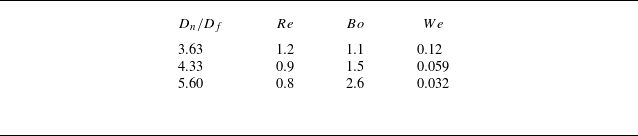
In what follows, we first validate our numerical formulation using the experiments in Ji et al. (Reference Ji, Sadeghpour, Ju and Bertozzi2020) for the configuration in figure 3(a) corresponding to a film flow over a flat fibre. Numerical simulations have been performed for three values of
 $D_n/D_f = 3.63$
,
 $4.33$
and
 $5.60$
that correspond to different
 $Re$
,
 $Bo$
and
 $We$
numbers given in table 2. Figure 10 shows the variation in the spacing between the fluid beads on the fibre,
 $\lambda _b/D_f$
, with increasing
 $D_n/D_f$
that is in good agreement with the experimental observations of Ji et al. (Reference Ji, Sadeghpour, Ju and Bertozzi2020). The corresponding interface profiles are presented in the insets given in figure 10(a). The interface profile from the numerical simulations are shown in red and are drawn over the experimental observations from Ji et al. (Reference Ji, Sadeghpour, Ju and Bertozzi2020). All the features of the instability of fluid flow on a fibre, such as healing length (length of the fibre over which instability develops to form droplets; see Duprat et al. Reference Duprat, Ruyer-Quil, Kalliadasis and Giorgiutti-Dauphiné2007), amplitude and wavelength of the fluid beads and their variation with increase in
 $D_n/D_f$
, are captured accurately using the current numerical formulation. Additionally, figure 10(b) presents a comparison between the numerical simulations and the experimental results from the present study for two Reynolds numbers, Re = 0.14 and Re = 0.16. The droplet spacing and interface profiles obtained from the simulations closely match those observed experimentally, further validating the accuracy of the numerical approach under the current experimental conditions.
Non-dimensional parameters calculated based on the velocities in the experiments of Ji et al. (Reference Ji, Sadeghpour, Ju and Bertozzi2020).

(a) Comparison of numerical simulations (filled circles) with the experimental results of Ji et al. (Reference Ji, Sadeghpour, Ju and Bertozzi2020) (filled black squares). Variation in the droplet spacing (
 $\lambda _b/D_f$
) with nozzle diameter (
 $D_n/D_f$
) is shown for three different configurations. Corresponding interface profiles have also been compared, as shown in the inset figures. Interface profiles obtained from numerical simulations (marked in red) are superimposed on the experimental images. (b) Comparison of numerical simulations with the experiments in the present study for
 $D_n/D_f = 14.28$
and
 $Re = 0.14$
and 0.16.

In the reduced-order numerical model proposed in Ji et al. (Reference Ji, Sadeghpour, Ju and Bertozzi2020), a van der Waals based repulsion term (for wetting fluids), using a stabilising Hamaker constant, was employed to prevent the film thickness becoming negative (that is to prevent the film profile penetrating the fibre). For this a critical minimum film thickness (
 $\epsilon _p$
) was chosen and a corresponding critical value of the Hamaker constant was derived using the stability condition for a stable coating of thickness
 $\epsilon _p$
. A sensitivity analysis presented in Ji et al. (Reference Ji, Sadeghpour, Ju and Bertozzi2020) showed the dependence of droplet spacing and velocity on the choice of
 $\epsilon _p$
. An appropriate value of
 $\epsilon _p$
was required for different flow rates. Typical values of
 $\epsilon _p$
chosen were in the range 0.150–3 mm, which correspond to a thickness much larger than the thickness of
 $100\, {\textrm {nm}}$
above which van der Waals forces are known to have little effect on the dynamics of the film. In contrast to that, in the Navier–Stokes based model used in the present study, we do not employ any such a model parameter. The thin regions are sufficiently resolved.
We now present numerical results for flow over a fibre with a solid bead on the fibre. In particular, we perform numerical simulations to study the effect of blockage ratio (
 $\textit{BR}$
) and multiple blockages for the set of parameters considered in this study, which are 0, 0.5, 0.75 and 0.95. Bead geometry specified by (3.2) and illustrated in the figure 3(b) closely mimics the experimental geometry discussed in the previous section. In order to study the effect of
 $\textit{BR}$
, we choose
 $Re=0.9$
, which corresponds to Rayleigh–Plateau instability regime for
 $\textit{BR}=0$
shown in the spatio-temporal graph in figure 11(a). The spatio-temporal graph shows a short healing length (
 $h_0$
) near the nozzle and subsequently uniformly spaced wave crests (droplets) in the entire time domain of the simulation with
 $\lambda =5.5$
moving with a speed of
 $54$
mm s−1. The interface profile corresponding to
 $t=2.5$
s is shown adjacent to the spatio-temporal map in figure 11(a). The effect of the presence of a solid bead on a fibre is shown in the spatio-temporal evolution maps in figure 11(b–d). Solid beads of different sizes are placed at
 $30R_n$
downstream from the nozzle. Droplet formation upstream of the solid bead is the same as the one with
 $\textit{BR} = 0$
(cylindrical fibre). Figure 11(b) shows the evolution of the fluid film for
 $\textit{BR}=0.5$
. Upstream of the bead, the droplets initially form in the Rayleigh–Plateau regime with a regular spacing. However, once the droplets cross over the bead, after a short initial transience, the droplets move again with uniform spacing (see
 $t \gt 2.25$
s). The slope of the crest lines indicate that after the initial transient the droplet speed in the quasi-steady state remains unaffected by the bead. The interface profile of the film shown adjacent to the graph corresponds to
 $t = 2.5$
s. Clearly, the droplet size sufficiently downstream of the bead is similar to the droplets upstream of the bead. Also, at the solid bead, droplets slow down and merge with the droplets in the upstream and subsequently break off and continue travelling downstream with a uniform speed.
Spatio-temporal graph for different beads with (a)
 $\textit{BR} = 0.0$
(cylinderical fibre), (b)
 $\textit{BR} = 0.5$
, (c)
 $\textit{BR} = 0.75$
and (d)
 $\textit{BR} = 0.95$
. Other parameters used for the numerical simulations are
 $D_n/D_f = 4.32$
,
 $Re = 0.90$
,
 $Bo = 1.5$
and
 $We = 0.059$
. Corresponding interface profiles at
 $t = 2.50\, \text{s}$
are shown adjacent to the spatio-temporal graphs for different
 $\textit{BR}$
values.

Figure 11(c) shows the spatio-temporal map corresponding to
 $\textit{BR}=0.75$
. Similar to the
 $\textit{BR}=0.5$
case, droplet formation and motion upstream of the bead remain unaffected. However, the influence of the presence of a solid bead on the film in the downstream is clearly evident. At the solid bead, a healing length region (
 $h_0$
), similar to the one at the nozzle, is observed. Further, we observe merging of droplets at regular intervals downstream of the bead as indicated by the merging crest lines in the spatio-temporal graph. Droplets also show irregular spacing and velocities suggested by the slope of the crest lines. These features are similar to the ones observed in experiments (see figure 6). These spatio-temporal maps indicate periodic merging after every third droplet at a fixed location. Further increase in
 $\textit{BR}$
to
 $0.95$
increases the number of merging events downstream of the solid bead, as shown in figure 11(d). The speed of the droplets moving downstream at
 $z = 40$
mm is given by 54 , 52 , 50 and 47 mm s−1, for
 $\textit{BR} = 0, 0.5, 0.75$
and
 $0.95$
, respectively.
To further investigate the role of the single bead of fibre on the redistribution of axial Kinetic energy, we compute the temporal evolution of the difference in axial kinetic energy flux,
 $\dot{E}_{\textit{KE}}(x, t)$
, between two axial positions.
The kinetic energy flux at a given location is defined as
 \begin{align} \dot{E}_{\textit{KE}}(x, t)= \int _{r_f}^{r_f + h(x,t)} 2\pi y\, {\boldsymbol{\cdot}}\, \frac {1}{2} \rho \, U^3(y, t) \, {\textrm d}y, \end{align}
where
 $U(y, t)$
is the axial velocity,
 $h(x,t)$
is the film thickness and
 $r_f$
is the fibre radius. This calculation is based on simulation data extracted along the vertical plane at
 $x = 20\,\textrm{}$
,
 $x = 30\,\textrm{}$
and
 $x = 45\,\textrm{mm}$
.
Figure 12(a) shows
 $\dot{E}_{\textit{KE}}(x, t)$
for various
 $\textit{BR}$
, computed between
 $x = 30\,\textrm{}$
and
 $x = 20\,\textrm{mm}$
, and between
 $x = 45\,\textrm{}$
and
 $x = 20\,\textrm{mm}$
in figure 12(b). For the flat fibre (
 $\textit{BR}$
= 0),
 $\dot{E}_{\textit{KE}}(x, t)$
shows periodic, high-amplitude oscillations, consistent with the Rayleigh–Plateau regime where a uniform train of droplets forms with little dissipation, as shown in figure 11(a) . In all the simulations, bead is centred at 27.9 mm downstream of the nozzle.
As the blockage ratio,
 $\textit{BR}$
, increases, the amplitude of
 $\dot{E}_{\textit{KE}}(x, t)$
decreases, indicating energy loss due to the interaction between the film and the bead. Figure 12 shows the variation in the difference in the kinetic energy flux (between locations
 $x_d$
and
 $x_u = 20\, {\rm mm}$
, downstream and upstream, respectively) with time. The difference is computed for two locations, one immediately downstream of the bead at
 $30\, {\rm mm}$
(figure 12
a) and another further downstream at
 $45\,{\rm mm}$
(figure 12
b). For different
 $\textit{BR}$
, figure 12(a) shows that, although the kinetic energy difference continuously decreases with the increase in
 $\textit{BR}$
, indicating momentum loss due to the bead, the frequency of oscillations in the kinetic energy for
 $x_d = 30\, {\rm mm}$
still corresponds to the rate at which droplets arrive at the bead. However, for
 $x_d = 45\, {\rm mm}$
, the effect of droplet mergers is clearly seen in both droplet frequency and magnitude of the kinetic energy.
We have also performed additional simulations to study the influence of Reynolds number on the blockage ratio effects. As shown in figure 13, the film dynamics is influenced by
 $\textit{BR}$
at low Reynolds numbers. The capillary effects dominate at lower Re, while inertial effects at higher Re tend to suppress the influence of geometry.
Comparison of kinetic energy flux difference
 $\dot{E}_{\textit{KE}}(x, t)$
between two downstream locations relative to an upstream reference at
 $x = 20$
mm, for different blockage ratios (BR). (a)
 $\dot{E}_{\textit{KE}}(x, t)$
computed as the difference between
 $x_d = 30$
mm (downstream) and
 $x_u = 20$
mm (upstream). (b)Value of
 $\dot{E}_{\textit{KE}}(x, t)$
computed between
 $x_d = 45$
and
 $x = 20$
mm. These plots show how the difference in kinetic energy flux (
 $\dot{E}_{\textit{KE}}(x, t)$
) reduces as the flow moves downstream.

(a) Phase diagram showing the transition from the Rayleigh–Plateau regime to droplet merging as a function of blockage ratio (
 $\textit{BR}$
) and Reynolds number (Re). The transition is delayed at higher Re, indicating increased film stability. (b–e) Interface profiles at
 $\textit{BR}$
= 0, 0.5, 0.75 and 0.9, respectively, for two Reynolds numbers (Re = 0.9 and Re = 1.5), plotted at t = 3 s under fully developed conditions. The results highlight how both
 $\textit{BR}$
and Re influence the film instability.

Figure 14(a) shows a spatio-temporal graph for flow over a fibre with two solid beads with
 $\textit{BR} = 0.75$
placed at
 $z = 27$
and
 $z = 76$
mm, respectively. Velocity at the nozzle corresponds to
 $Re = 0.90$
. Interface profile adjacent to the graph corresponds to
 $t = 2.5$
s. These computations have been performed with a computational domain that is two times longer in the axial direction. Upstream of the bead, droplets are of uniform size (6.0 mm) and travel with a constant velocity (57 mm s−1). Flow disruption by the first bead results in irregular merger between droplets, thus modifying the size and spacing between the droplets. As the droplets encounter the second bead, there is further increase in their speed and sizes as indicated by the thickening of the crest lines and an increase in their slope. After the encounter with the second bead, we note ripples in the space between the droplets (as suggested by the faint streak lines merging with the crest lines). The speed of these ripples,
 $39$
mm s−1, corresponds to the viscous capillary speed
 $\gamma /\mu$
(43 mm s−1). Figure 14(b) shows the spatio-temporal graph for flow over a granular chain with beads placed at a spacing of approximately
 $7.25$
mm and radii corresponding to
 $\textit{BR} = 0.75$
. We note that, after a couple of beads, the droplet size and velocity stabilise and no further droplet mergers are observed in the downstream. The spacing between the solid beads of the granular chain is similar to the experimental results shown in figure 8.
Spatio-temporal graph for the film flow at
 $Re=0.90$
on a fibre with (a) two solid beads placed at
 $z = 27$
and
 $76$
mm, (b) granular chain, both with
 $\textit{BR}=0.75$
. The corresponding interface profiles are shown adjacent to the spatio-temporal graphs at
 $t = 2.5\, \text{s}$
.

Figure 15 also shows the effect of the blockage ratio and location of the bead with respect to the healing length. Spatio-temporal graphs for
 $L_p = 10D$
, and
 $\textit{BR} = 0.5$
(figure 15
a) and
 $\textit{BR} = 0.75$
(figure 15
b) are very similar, indicating that the evolution of the instability is not affected significantly by the bead size (blockage ratio) if placed within the healing length. However, we note that, when the solid beads are placed within the healing length of the liquid film near the nozzle, the blockage has a coarsening effect on the droplet spacing in stark contrast to the film evolution shown in figure 11 for the same
 $\textit{BR}$
values.
Spatio-temporal graph showing the effect of the location of the solid beads on the evolution of the film for
 $\textit{BR}$
ratios: (a)
 $\textit{BR}=0.5$
, (b)
 $\textit{BR}=0.75$
and (c) kinetic energy flux variation upstream and downstream of the solid bead located at 0.2 mm for
 $\textit{BR} = 0.75$
, computed from axisymmetric numerical simulations using Gerris. The upstream
 $\dot{E}_{\textit{KE}}(x, t)$
(green) at
 $x=0.2$
mm, which lies within the healing length, remains nearly constant throughout the time window from 1.5 to 2.5 s. In contrast, the downstream
 $\dot{E}_{\textit{KE}}(x, t)$
(red) at
 $x=30$
mm exhibits strong periodic oscillations associated with droplet formation past the bead.

Further figure 15(c) is shown to examine the variation in axial kinetic energy flux upstream of the bead within the healing length. The figure shows that kinetic energy flux at x = 0.2 mm remains constant in figure 15(c). This indicates a stable flow can be observed within the healing length. This implies that the influence of a gradual change in bead position within the healing length does not significantly alter the transition dynamics. Therefore, the regime transition is not sensitive to small variation in bead placement within this region.
The present study explores three different experimental configurations to analyse the influence of bead spacing on film evolution: (i) a single bead placed downstream at 27.9 mm from the nozzle tip, (ii) two beads with a separation of 25 mm and (iii) closely spaced beads with a separation of 7.2 mm (figure 6). These configurations were carefully chosen to highlight major dynamical changes observed. Configurations isolate film behaviour downstream of beads in the Rayleigh–Plateau regime and the onset of the droplet merging regime. We have also performed additional experiments to study the effect of placing the bead in the healing length (see figure 16). The influence of the bead location relative to the healing length. The present experimental and numerical study was conducted in the Rayleigh–Plateau regime, consistent with the Reynolds number range studied by Ji et al. (Reference Ji, Sadeghpour, Ju and Bertozzi2020). In this regime, the healing length increases with increasing Reynolds number, which implies a longer development region for droplet formation downstream of the nozzle. When beads were positioned within the healing length, we observed a significant coarsening of the droplet pattern, both in experiments and consistently with the numerical results. This coarsening becomes more prominent with increasing
 $\textit{BR}$
, indicating that the flow obstruction introduced within the healing region leads to stronger variations in the droplet train.
However, the evolution of the axial kinetic energy flux difference, shown in figure 12, reveals a transition from periodic, high-amplitude oscillations. This behaviour is characteristic of the Rayleigh–Plateau regime, where a stable train of droplets forms on a flat fibre. Film evolution with
 $\textit{BR}$
= 0.75,
 $\Delta \dot{E}_{\textit{KE}}$
remains periodic near the bead at x = 30 mm, but becomes irregular farther downstream at x = 45 mm. This transition reflects droplet merging events and the formation of a secondary healing region. These observations highlight that the bead acts as a localised spatial perturbation, modulating the underlying periodic film. Motivated by this behaviour, we now investigate the effect of
 $\textit{BR}$
as a perturbation to the flow by studying the perturbation introduced by the bead to the flow.
Experimental spatio-temporal graph showing the effect of the location of the solid bead on the evolution of the film for BR ratios: (a)
 $\textit{BR}$
= 0.34 and (b)
 $\textit{BR}$
= 0.68, Re = 0.123.

(a) Variations in flow rate (
 $Q$
) at
 $z=20$
mm (upstream of the blockage) and at
 $z=30$
mm (just downstream of the blockage) are shown as a function time (s). (b) Corresponding FFTs of the two time series.

(a) Spatio-temporal evolution of the film flow for inlet velocity perturbations obtained at
 $z=30$
mm for
 $\textit{BR}=0.75$
. Film height variation and the corresponding FFT for
 $\textit{BR} = 0.75$
(blue) and for cylindrical fibre with perturbation in the inlet velocity (red) at (b)
 $z = 10$
mm and (c)
 $z=80$
mm.

Spatio-temporal chart for different values of inlet velocity perturbation amplitude and frequency on the film evolution.

Figure 17 shows the variation in the axial velocity with time at
 $z = 20$
and 30 mm. Perturbations closer to the bead are of higher magnitude compared with those downstream. The corresponding FFT shows a peak at 9.34 Hz and a secondary peak at 18.69 Hz. We employ this frequency to the perturbations at the inlet and compare the solutions so obtained with those for the bead. The following velocity field is imposed at the inlet and flow evolution is observed for flow over a flat fibre
 \begin{align} V = v_0 \left ( 1 + \epsilon _0 \left ( \sin (\omega _1 t) + \frac {A_2}{A_1} \sin (\omega _2 t) + \frac {A_3}{A_1} \sin (\omega _3 t) + \cdots \right ) \right ). \end{align}
Each term is scaled by a factor that relates its amplitude
 $A_n$
to the amplitude
 $A_1$
of the first frequency component. When the inlet is perturbed with the frequencies obtained from the flow rate variation in the above form, the system shows behaviour in the droplet merging regime similar to
 $\textit{BR}=0.75$
, as shown in the figure 18. We have shown that a bead located downstream (at
 $x \times 15D_f$
from the nozzle) introduces a localised spatial perturbation that significantly affects the film evolution. Following the theoretical investigations of Shkadov & Sisoev (Reference Shkadov and Sisoev2004), Ruyer-Quil et al. (Reference Ruyer-Quil, Treveleyan, Giorgiutti-Dauphiné, Duprat and Kalliadasis2008) and Trifonov (Reference Trifonov2017), we understand that, from a number of possible solutions, the physical system of flow over a cylindrical fibre picks up the most stable solution, which as discussed earlier can be categorised as Rayleigh–Plateau or droplet merging or wavy regime depending upon the inlet conditions. It has been shown that perturbations to the velocity field at the inlet can result in transition between the regimes, resulting in convective to absolute instability (Duprat et al. Reference Duprat, Ruyer-Quil and Giorgiutti-Dauphiné2009). Here, in this study, we first characterise the perturbation to the flow introduced by the placement of a bead. Subsequently, we prescribe the perturbation in the velocity field so obtained at the inlet of the nozzle for a cylindrical fibre and analyse whether the regimes (droplet merging events) are qualitatively and quantitatively similar to those observed in the downstream of the bead. Figure 18 shows the spatio-temporal evolution due to the perturbed inlet flow (see Sisoev et al. Reference Sisoev, Craster, Matar and Gerasimov2006; Duprat et al. Reference Duprat, Ruyer-Quil and Giorgiutti-Dauphiné2009). Comparing the evolution with those for the bead shown in figure 14(a) suggests that the flow solutions obtained due to the perturbation introduced by the bead correspond to those for the inlet perturbation of a certain frequency. The dominant frequency, however, remains the same as that for the flat fibre. Figures 18(b) and 18(c) show the corresponding film height evolution and the frequency plot.
Figure 19 shows the variation in the solution obtained for different perturbations in the inlet velocities. For smaller-amplitude perturbations the solution does not deviate much but for higher-amplitude perturbations there is significant deviation from the solution without perturbations. Therefore, by imposing perturbations of certain frequency and amplitude of the inlet perturbations, desired flow over a fibre can be obtained.
5. Conclusions
Experimental investigation of the flow over a fibre with a corrugation (a rigid bead) shows that droplet mergers occur at the protuberances resulting in a change in the spacing and speed of the droplets. The initial sharp distribution of length scales (FFT of the film height at a given location indicating variation in droplet spacing) transforms into a much wider distribution due to drop mergers. The introduction of multiple such corrugations leads to a progressive change in the spacing distribution with the axial coordinate, with a significant change in the peak and the spread of the length scales. The spacing between the droplets increases, suggesting a shift in the regime from inertial to inertialess toward the Rayleigh–Plateau regime. When the spacing between the rigid beads is much shorter (granular chain) than the spacing between droplets for a smooth fibre, the spacing spectrum immediately after the first bead essentially remains unchanged and is given by the spacing between the beads.
In order to analyse if the introduction of beads is similar to a perturbation in velocity at the nozzle for a smooth fibre, we obtain the dominant frequency and the corresponding amplitude of the mean axial velocity immediately after the rigid bead and introduce them at the nozzle for a smooth fibre. We show that the change in the spacing so obtained is qualitatively similar to that in the presence of a rigid bead, suggesting that the stationary solutions of droplet formation selected for higher-amplitude perturbations are different from those corresponding to the instability for an infinitesimal perturbation.
This study would be useful in coating, film cooling and desalination applications involving corrugated fibres. We note that in coating applications it is important to know the required flow rate for a coating of a particular thickness. Moreover, it is critical to understand whether the coating process is resulting in a uniform film thickness. We believe the current study provides insights into the flow over corrugated fibres encountered in a variety of applications. In desalination applications, it is imperative to remove and collect the condensed liquid at a fast rate. An understanding of the flow dynamics would thus be useful in desalination systems as well (see Dietze Reference Dietze2019; Bonart et al. Reference Bonart, Rajes, Jung and Repke2020; Sadeghpour Reference Sadeghpour2020).
Acknowledgements
Authors thank Professor S. Kalliadasis for invaluable insights into the problem.
Declaration of interests
The authors report no conflict of interest.
Appendix A. Grid Independence Study
A study of the influence of the mesh was conducted to rule out the effect of spatial resolution on the film evolution. Figure 20 compares the film interface profiles at fully developed conditions between grid levels 7 and 8 (maximum refinement regions), corresponding to smallest grid sizes
 $\Delta x = 9.41\, $
and
 $4.71\, \mu$
m, respectively. All simulation results presented in this study correspond to level 8.
Film interface profiles at fully developed conditions compared between grid levels 7 and 8 (maximum refinement regions), corresponding to smallest grid sizes
 $\Delta x = 9.41\, $
and
 $4.71\, \mu$
m, respectively. All simulation results presented in this study correspond to level 8.