1 Introduction
In 1940, Görtler (Reference Görtler1940) discovered a flow instability in the form of counter-rotating longitudinal vortices caused in boundary layers over concave surfaces by an imbalance between pressure and centrifugal forces. These perturbations have thereafter been called Görtler vortices. Hall (Reference Hall1983, Reference Hall1990) identified the key features for the rigorous theoretical description of the Görtler vortices. The full Navier–Stokes equations can be simplified to the parabolic three-dimensional boundary layer equations in the limit of large Reynolds numbers, where the effect of curvature is distilled in the Görtler number, i.e., the ratio between the squared Reynolds number and the dimensionless radius of curvature, appearing in a convection term of the wall-normal momentum equation. The mathematical consequence of the parabolic character of the system is that, to describe the flow correctly, these equations must be complemented by rigorous initial conditions (near the leading edge) and outer boundary conditions (free stream and wall), i.e., the receptivity to external disturbances must be included in the formulation. Hall (Reference Hall1982) thus proved that an eigenvalue formulation, for example following from the parallel-flow assumption and leading to a system of ordinary differential equations, is only valid as an asymptotic approximation for the study of Görtler flows in the limits of large Görtler number and short spanwise wavelength. Hall (Reference Hall1983) also showed the strong dependence of the solution on the initial conditions, thereby confirming that a unique neutral curve does not exist if the initial conditions vary.
The correct mathematical description of the influence of low-frequency free-stream disturbances on flat-plate boundary layers, which translates into the unequivocal form of the initial and free-stream boundary conditions, was formulated by Leib, Wundrow & Goldstein (Reference Leib, Wundrow and Goldstein1999). Their theory focuses on the dynamics of streamwise-elongated perturbations inside the boundary layer, widely recognized as the cause of bypass transition, i.e., the route to turbulence where Tollmien–Schlichting (TS) waves do not play a significant role. These boundary layer perturbations take the form of streaky structures and are often called Klebanoff modes. Wu, Zhao & Luo (Reference Wu, Zhao and Luo2011) extended the flat-plate theory of Leib et al. to study the linear evolution of incompressible Görtler vortices subject to free-stream vortical disturbances which, in their initial linear stage, resemble Klebanoff modes. Thanks to these theoretical advancements, the Görtler flow is precisely and uniquely linked to the characteristics of the free-stream disturbances. The issue of the strong dependence of the Görtler vortices on the arbitrary initial conditions shown by Hall (Reference Hall1983) has therefore been resolved for flows exposed to free-stream disturbances, while the receptivity to wall roughness has been studied by Bassom & Seddougui (Reference Bassom and Seddougui1995) and by Sescu & Thompson (Reference Sescu and Thompson2015). However, Görtler-flow neutral curves, i.e., curves in the parameter space which separate regions of growth and decay of the boundary layer perturbations, were not computed by Wu et al. (Reference Wu, Zhao and Luo2011) and it thus remains an open problem. This is in contrast to the search for the neutral curve of the TS waves, which was solved by Tollmien (Reference Tollmien1929).
We use the receptivity–stability framework developed by Wu et al. (Reference Wu, Zhao and Luo2011) to achieve three objectives. First we compute the neutral curves for different Görtler numbers and characteristics of the free-stream disturbance, for both Klebanoff modes and Görtler vortices. These neutral curves define the regions of stability from the leading edge for the entire range of the spanwise wavenumber and low frequency. The flat-plate scenario is included in the analysis. The neutral curves also identify the minimum Görtler number below which the perturbation does not develop into Görtler vortices even in the presence of curved surfaces and the maximum Görtler number above which Klebanoff modes, which are always present near the leading edge, evolve directly into Görtler vortices. The study of the neutral curve is also relevant because it finds the conditions for which the Görtler instability affects the wall-shear stress significantly. Extending the receptivity analysis of Wu et al., we propose a modified receptivity coefficient which allows us to obtain the maximum amplitude of the boundary layer perturbations from the local eigenvalue solution. Finally, we discuss the use of the
 $N$
-factor approach, widely used by engineers for the prediction of transition to turbulence (Van Ingen Reference Van Ingen1956; Jaffe, Okamura & Smith Reference Jaffe, Okamura and Smith1970), when the receptivity of the boundary layer to free-stream disturbances is included in the formulation.
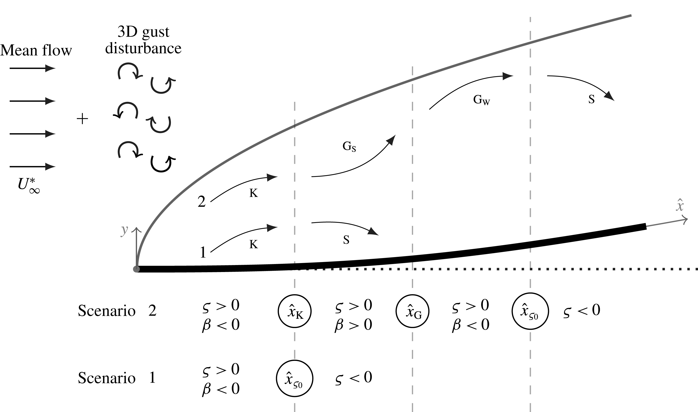
Schematic of growth and decay of boundary layer perturbations based on the parameters
 $\unicode[STIX]{x1D70D}$
and
 $\unicode[STIX]{x1D6FD}$
defined in (2.3). The sketch represents
 $\text{K}$
-vortices, Görtler vortices with strong growth
 $\text{G}_{\text{S}}$
, Görtler vortices with weak growth
 $\text{G}_{\text{W}}$
, and stable flows S. In the steady case, scenario 1 is typical for
 $G<G_{B}=10.9$
, while scenario 2 is typical for
 $G>G_{C}=17$
.

2 Mathematical framework
2.1 Flow definition and scaling
We consider an incompressible uniform flow of velocity
 $U_{\infty }^{\ast }$
past a concave plate with constant radius of curvature
 $r^{\ast }$
. The flow is shown in figure 1 and hereinafter the asterisk
 $^{\ast }$
identifies dimensional quantities. A boundary layer forms over the curved plate. Free-stream vortical disturbances are passively advected by the uniform free-stream flow and are modelled as three-dimensional vortical disturbances of the gust type, which, sufficiently upstream and away from the plate, have the form
 $$\begin{eqnarray}\boldsymbol{u}-\boldsymbol{i}=\unicode[STIX]{x1D716}\hat{\boldsymbol{u}}^{\infty }\;\text{e}^{\text{i}(\boldsymbol{k}\boldsymbol{\cdot }\boldsymbol{x}-k_{x}Re\hat{t})}+\text{c.c.},\end{eqnarray}$$
where
 $\unicode[STIX]{x1D716}$
is a small parameter,
 $\boldsymbol{x}=\{x,y,z\}$
denotes the streamwise, wall-normal and spanwise directions,
 $\boldsymbol{k}=\{k_{x},k_{y},k_{z}\}$
defines the wavenumber vector,
 $\hat{\boldsymbol{u}}^{\infty }=\{\hat{u} ^{\infty },\hat{v}^{\infty },{\hat{w}}^{\infty }\}$
is the amplitude of the free-stream disturbance, c.c. indicates the complex conjugate, and
 $\boldsymbol{i}$
is the unit vector of the streamwise direction. The wavenumber vector
 $\boldsymbol{k}$
and the velocity vector
 $\hat{\boldsymbol{u}}^{\infty }$
satisfy the solenoidal condition
 $\boldsymbol{k}\boldsymbol{\cdot }\hat{\boldsymbol{u}}^{\infty }=0$
. Lengths are scaled by
 $\unicode[STIX]{x1D6EC}_{z}^{\ast }=\unicode[STIX]{x1D706}_{z}^{\ast }/2\unicode[STIX]{x03C0}$
, where
 $\unicode[STIX]{x1D706}_{z}^{\ast }$
is the spanwise wavelength of the gust, velocities are scaled by
 $U_{\infty }^{\ast }$
, and the pressure is scaled by
 $\unicode[STIX]{x1D70C}^{\ast }{U_{\infty }^{\ast }}^{2}$
, where
 $\unicode[STIX]{x1D70C}^{\ast }$
is the density of the fluid. We define the Reynolds number
 $Re=U_{\infty }^{\ast }\unicode[STIX]{x1D6EC}_{z}^{\ast }/\unicode[STIX]{x1D708}^{\ast }\gg 1$
, where
 $\unicode[STIX]{x1D708}^{\ast }$
is the kinematic viscosity of the fluid, and the Görtler number
 $G=Re^{2}\unicode[STIX]{x1D6EC}_{z}^{\ast }/r^{\ast }=O(1)$
. The dimensionless spanwise wavenumber is
 $k_{z}=1$
and the frequency parameter is
 $k_{x}Re$
. Since the interest is in streamwise-elongated perturbations, the streamwise coordinate and time are scaled as
 $\hat{x}=x^{\ast }/(Re\unicode[STIX]{x1D6EC}_{z}^{\ast })$
and
 $\hat{t}=U_{\infty }^{\ast }t^{\ast }/(Re\unicode[STIX]{x1D6EC}_{z}^{\ast })$
, respectively. The boundary layer velocity and pressure
 $\boldsymbol{q}(\boldsymbol{x},t)=\{u,v,w,p\}(\boldsymbol{x},t)$
are decomposed into their mean
 $\boldsymbol{Q}(\boldsymbol{x})$
and perturbation
 $\boldsymbol{q}^{\prime }(\boldsymbol{x},t)$
as
 $\boldsymbol{q}=\boldsymbol{Q}+\unicode[STIX]{x1D716}\boldsymbol{q}^{\prime }$
. The mean flow is the Blasius boundary layer and the perturbations are
 $$\begin{eqnarray}\boldsymbol{q}^{\prime }=\text{i}k_{z}\breve{w}\left\{Re\bar{u},\,(2\hat{x})^{1/2}\bar{v},\,\frac{1}{\text{i}k_{z}}\bar{w},\,\frac{1}{Re}\bar{p}\right\}\text{e}^{\text{i}(k_{z}z-k_{x}Re\hat{t})}+\text{c.c.},\end{eqnarray}$$
where
 $\breve{w}\equiv {\hat{w}}^{\infty }+\text{i}k_{z}\hat{v}^{\infty }/(k_{x}^{2}+k_{z}^{2})^{1/2}=O(1)$
and only the three-dimensional part of the perturbation has been considered (Leib et al.
Reference Leib, Wundrow and Goldstein1999). In the limits of large Reynolds number
 $Re\gg 1$
, small perturbations
 $\unicode[STIX]{x1D716}\ll 1/Re$
, and low frequency
 $k_{x}\ll 1$
, the linearized unsteady boundary region (LUBR) equations for the perturbation flow are recovered by inserting the flow decomposition, along with (2.2), into the full Navier–Stokes and continuity equations and collecting
 $O(\unicode[STIX]{x1D716})$
terms. Details of the mathematical methodology are found in Leib et al. (Reference Leib, Wundrow and Goldstein1999) and Wu et al. (Reference Wu, Zhao and Luo2011). The LUBR equations are parabolic along the streamwise direction and are coupled with initial and boundary conditions derived through asymptotic matching with the oncoming free-stream vortical disturbances (Leib et al.
Reference Leib, Wundrow and Goldstein1999; Wu et al.
Reference Wu, Zhao and Luo2011). A second-order implicit finite-difference scheme has been used to solve the LUBR equations (Ricco & Wu Reference Ricco and Wu2007). The three parameters influencing the flow are
 $G$
,
 $k_{y}$
and
 $k_{x}Re$
. They account for the effects of curvature, ratio of the free-stream spanwise wavelength to the wall-normal wavelength, and frequency, respectively. To stress the importance of receptivity, we note that the solution is influenced by
 $k_{y}$
only through the initial and boundary conditions as
 $k_{y}$
does not appear in the LUBR equations (Leib et al.
Reference Leib, Wundrow and Goldstein1999; Wu et al.
Reference Wu, Zhao and Luo2011).
2.2 Neutral curve parameters
In previous representations of Görtler-flow neutral curves (Hall Reference Hall1990), the spanwise wavenumber, scaled by the boundary layer thickness, often appeared on the abscissa and a scaled Görtler number on the ordinate. In our scaling, this would translate into an
 ${\mathcal{X}}$
-
 ${\mathcal{G}}$
plane, where
 ${\mathcal{X}}=(2\hat{x})^{1/2}$
and
 ${\mathcal{G}}=G{\mathcal{X}}^{3}/\sqrt{2}$
, causing the neutral curve to collapse on a
 ${\mathcal{X}}^{3}$
curve, without fully revealing the flow behaviour, especially near the leading edge. We instead choose to represent the neutral curve in the
 $\hat{x}$
–
 $G$
plane so that for moderate
 $G$
the presence of Klebanoff modes and Görtler vortices is linked more distinctly to the flow stability. The neutral curves are thus found for different values of
 $k_{x}Re$
and
 $k_{y}$
in the
 $\hat{x}$
–
 $G$
plane.
The neutral curves are represented by the parameters
 $$\begin{eqnarray}\unicode[STIX]{x1D70D}(\hat{x})\equiv \frac{\text{d}E(\hat{x})}{\text{d}\hat{x}},\quad \unicode[STIX]{x1D6FD}(\hat{x})\equiv \frac{\text{d}^{2}|\bar{u}(\hat{x})|_{max}}{\text{d}\hat{x}^{2}},\end{eqnarray}$$
where
 $E(\hat{x})\equiv \int _{0}^{\infty }|\bar{u}(\hat{x},\unicode[STIX]{x1D702})|^{2}\text{d}\unicode[STIX]{x1D702}$
is the scaled perturbation energy divided by
 $(2\hat{x})^{1/2}$
(Hall Reference Hall1990) and
 $|\bar{u}(\hat{x})|_{max}\equiv \max _{\unicode[STIX]{x1D702}}|\bar{u}(\hat{x},\unicode[STIX]{x1D702})|$
is the maximum along
 $\unicode[STIX]{x1D702}=y/(2\hat{x})^{1/2}$
of the amplitude of the streamwise velocity perturbation. This definition of
 $\unicode[STIX]{x1D70D}(\hat{x})$
is well suited for the receptivity analysis since it retains the information from the perturbation amplitude. The latter would not enter the picture if the
 $\hat{x}$
-derivative of the energy were normalized by the energy itself, as in Hall (Reference Hall1990). Only the
 $|\bar{u}|$
component is used to define the scaled perturbation energy in (2.3) because the physical streamwise velocity component for the Görtler vortices is much larger than the transverse velocity components (Wu et al.
Reference Wu, Zhao and Luo2011).
Figure 1 summarizes how the instabilities are categorized according to (2.3). The flow is unstable for
 $\unicode[STIX]{x1D70D}>0$
and stable for
 $\unicode[STIX]{x1D70D}<0$
, with
 $\unicode[STIX]{x1D70D}=0$
defining the neutral points located at
 $\hat{x}=\hat{x}_{\unicode[STIX]{x1D70D}_{0}}$
. Since curvature effects are not at work near the leading edge, the boundary layer perturbations start growing from the leading edge as Klebanoff modes, herein labelled
 $\text{K}$
-vortices, for which
 $\unicode[STIX]{x1D70D}>0$
,
 $\unicode[STIX]{x1D6FD}<0$
. Depending on
 $G$
,
 $k_{x}Re$
and
 $k_{y}$
,
 $\text{K}$
-vortices can either become stable downstream of
 $\hat{x}=\hat{x}_{\unicode[STIX]{x1D70D}_{0}}$
or turn into Görtler vortices at
 $\hat{x}=\hat{x}_{\text{K}}$
, where
 $\unicode[STIX]{x1D6FD}=0$
and
 $\unicode[STIX]{x1D6FD}^{\prime }(\hat{x})>0$
, with the prime indicating the derivative with respect to
 $\hat{x}$
. The Görtler vortices are characterized by an initial strong growth, for which
 $\unicode[STIX]{x1D6FD}>0$
(
 $\text{G}_{\text{S}}$
-vortices). When
 $\unicode[STIX]{x1D6FD}=0$
and
 $\unicode[STIX]{x1D6FD}^{\prime }<0$
at
 $\hat{x}=\hat{x}_{\text{G}}$
, the local growth rate is maximum and downstream their growth weakens as
 $\unicode[STIX]{x1D6FD}<0$
(
 $\text{G}_{\text{W}}$
-vortices), until they eventually stabilize downstream of
 $\hat{x}=\hat{x}_{\unicode[STIX]{x1D70D}_{0}}$
.
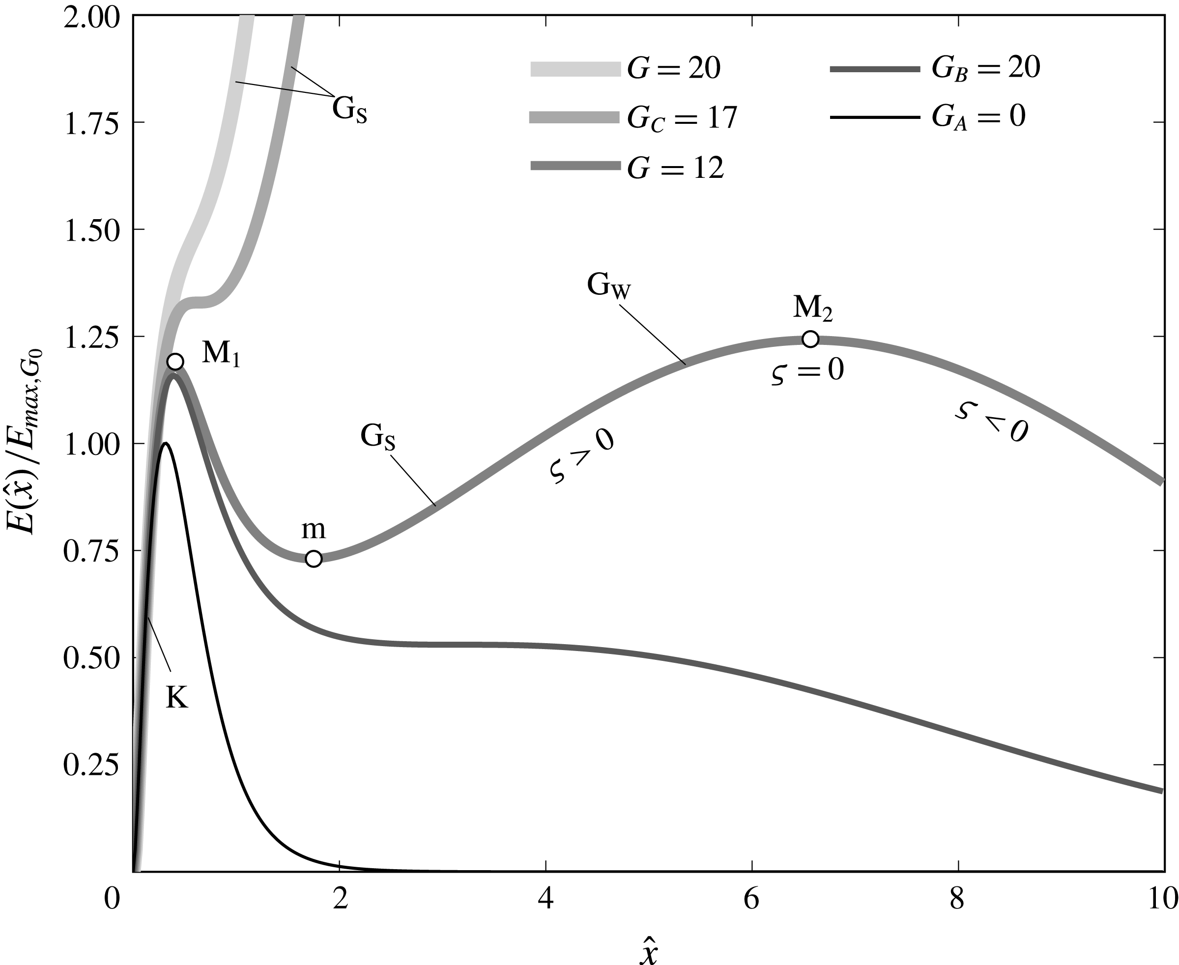
Perturbation energy
 $E(\hat{x})$
normalized by
 $E_{max,G_{0}}$
, the maximum value of
 $E$
for
 $G=0$
, as a function of
 $\hat{x}$
for
 $k_{x}Re=0$
and
 $k_{y}=2$
.

3 Results
3.1 Downstream evolution of the disturbance energy
The scaled perturbation energy
 $E(\hat{x})$
of both
 $\text{K}$
-vortices and Görtler vortices, normalized by the maximum value
 $E_{max,G_{0}}\equiv \max _{\hat{x}}|E(\hat{x})|_{G=0}$
for
 $G=0$
, is shown in figure 2 as a function of
 $\hat{x}$
for
 $k_{x}Re=0$
and
 $k_{y}=2$
. Energy maxima,
 $\text{M}_{1}$
and
 $\text{M}_{2}$
, and minima
 $\text{m}$
identify stable conditions, i.e., where
 $\unicode[STIX]{x1D70D}=0$
. Three critical Görtler numbers occur for this configuration, i.e.,
 $G_{A}$
,
 $G_{B}$
and
 $G_{C}$
. In the flat-plate case, for which
 $G=G_{A}=0$
, only
 $\text{K}$
-vortices are present. They start growing from the leading edge and then dissipate rapidly due to viscosity (Leib et al.
Reference Leib, Wundrow and Goldstein1999) as in scenario 1 of figure 1. As the curvature is introduced, the imbalance between pressure and centrifugal forces energizes the boundary layer perturbation. Only for
 $G>G_{B}=10.9$
do the Görtler vortices become unstable as secondary growing disturbances after the viscous decay of the
 $\text{K}$
-vortices. A new maximum
 $\text{M}_{2}$
thus emerges. Following the evolution of the perturbation for
 $G=12$
, figure 2 shows that
 $\text{K}$
-vortices represent the initial instability of the boundary layer, which starts stabilizing at
 $\text{M}_{1}$
. After the viscous decay, the onset of the Görtler vortices causes the boundary layer to become unstable again at
 $\text{m}$
. Their initial strong growth
 $\text{G}_{\text{S}}$
shifts into a weak growth
 $\text{G}_{\text{W}}$
at
 $\hat{x}=\hat{x}_{\text{G}}$
before ultimately stabilizing again at
 $\text{M}_{2}$
. In the range
 $G_{B}<G<G_{C}=17$
both instabilities are thus present. Figure 2 also shows that for
 $G>G_{C}$
the
 $\text{K}$
-vortices turn into Görtler vortices directly without the intermediate viscous decay: the first peak
 $\text{M}_{1}$
in the scaled energy distribution is no longer present and the perturbation thus evolves as in scenario 2 in figure 1.
3.2 Neutral curves
We can now obtain a neutral stability curve in the
 $\hat{x}$
–
 $G$
plane for each pair of parameters (
 $k_{x}Re$
,
 $k_{y}$
).
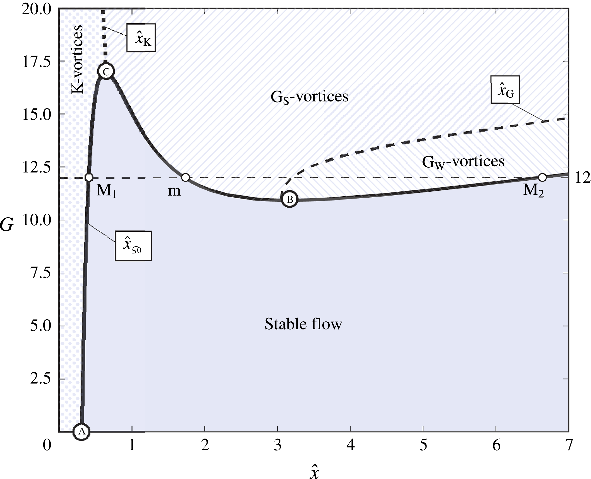
Neutral stability curve,
 $\hat{x}=\hat{x}_{\unicode[STIX]{x1D70D}_{0}}$
(——), and curves at which the
 $\text{K}$
-vortices turn into
 $\text{G}_{\text{S}}$
-vortices,
 $\hat{x}=\hat{x}_{\text{K}}$
(
 $\cdots \cdots$
), and the
 $\text{G}_{\text{S}}$
-vortices turn into
 $\text{G}_{\text{W}}$
-vortices,
 $\hat{x}=\hat{x}_{\text{G}}$
(- - - -), for
 $k_{x}Re=0$
,
 $k_{y}=2$
.

Curve at which the
 $\text{K}$
-vortices turn into
 $\text{G}_{\text{S}}$
-vortices,
 $\hat{x}=\hat{x}_{\text{K}}$
(
 $\cdots \cdots$
), and neutral stability curve,
 $\hat{x}=\hat{x}_{\unicode[STIX]{x1D70D}_{0}}$
(——), for
 $k_{x}Re=0$
,
 $k_{y}=2$
, and large
 $G$
numbers. The experimental values by Boiko et al. (Reference Boiko, Ivanov, Kachanov and Mischenko2010) (

 $G\gg 1$
,
 $\hat{x}_{I}=O(G^{-2/3})$
(— ⋅ —) and
 $\hat{x}_{II}=O(G^{-2/5})$
(— ⋅ ⋅ —), are shown.

3.2.1 Steady Görtler-flow scenario
The neutral curve for
 $k_{x}Re=0$
and
 $k_{y}=2$
is shown in figure 3. The continuous black line represents the neutral curve, the black dotted line indicates the streamwise location
 $\hat{x}_{\text{K}}$
where
 $\text{K}$
-vortices turn into Görtler vortices directly, and the black dashed line represents the streamwise location
 $\hat{x}_{\text{G}}$
where the growth of the Görtler vortices shifts from strong to weak. Three critical points of the neutral curve, A, B, C, are shown in figure 3. Point A indicates the
 $\hat{x}$
location downstream of which the
 $\text{K}$
-vortices are stable for
 $G=0$
, while point B denotes the
 $\hat{x}$
location of the local minimum of the neutral curve, corresponding to the Görtler number (
 $G_{B}=10.9$
) below which only
 $\text{K}$
-vortices exist. Point C indicates the
 $\hat{x}$
location of the local maximum of the neutral curve corresponding to the Görtler number (
 $G_{C}=17$
) above which
 $\text{K}$
-vortices shift directly to Görtler vortices.
The neutral curve shows that
 $\text{K}$
-vortices always exist near the leading edge for any Görtler number and that increasing the Görtler number strengthens the inviscid nature of the Görtler instability, thereby causing the unstable region to expand rapidly. As the curvature increases, the point
 $\text{m}$
, also shown in figure 2, moves closer to the leading edge and eventually merges with
 $\text{M}_{1}$
for
 $G=G_{C}$
. For
 $G>G_{C}$
, the boundary layer is unstable from the leading edge as
 $\text{K}$
-vortices turn into Görtler vortices at
 $\hat{x}=\hat{x}_{\text{K}}$
. If the perturbation energy were defined by integrating
 $|\bar{u}|$
over
 $y$
for the definition of
 $\unicode[STIX]{x1D70D}$
, the neutral curve would be slightly shifted to lower
 $G$
but would retain its shape.
In the limit
 $G\gg 1$
, the asymptotic analysis of Wu et al. (Reference Wu, Zhao and Luo2011) shows that the perturbation undergoes two pre-modal stages before it exhibits exponential growth. The
 $\text{K}$
-vortices experience a first change in their dynamics when
 $\hat{x}_{I}=O(G^{-2/3})$
, i.e., when curvature effects start influencing the pressure field which, at this stage, is decoupled from the velocity field. Further downstream, the second pre-modal stage ensues when
 $\hat{x}_{II}=O(G^{-2/5})$
, i.e., when the wall-normal gradient of the pressure perturbations becomes comparable with the convection terms, thus defining the onset of the Görtler instability. Figure 4 depicts the extension of figure 3 for large
 $G$
numbers at small
 $\hat{x}$
. The red dash-dotted lines in figure 4 indicate the large-
 $G$
pre-modal asymptotic limits, clearly showing that
 $\hat{x}_{I}<\hat{x}_{\text{K}}<\hat{x}_{II}$
as
 $G$
increases. This confirms that
 $\unicode[STIX]{x1D6FD}$
is appropriate for assessing the location where
 $\text{K}$
-vortices turn into Görtler vortices and our approach is consistent with the large-
 $G$
analysis of Wu et al. (Reference Wu, Zhao and Luo2011). In particular, we find that
 $\hat{x}_{\text{K}}=O(G^{-0.52})$
in the range
 $10^{4}<G<10^{6}$
.
It is also important to set experimental results of Görtler vortices within our theoretical framework. Görtler vortices induced by free-stream disturbances over concave surfaces were experimentally studied by Boiko et al. (Reference Boiko, Ivanov, Kachanov and Mischenko2010) for a wide range of parameters:
 $r^{\ast }=8.37~\text{m}$
,
 $\unicode[STIX]{x1D706}_{z}^{\ast }=0.008,0.012,0.024$
, and unit Reynolds number
 $Re_{U}^{\ast }=U_{\infty }^{\ast }/\unicode[STIX]{x1D708}^{\ast }=6\times 10^{5}~\text{m}^{-1}$
. As expected, in their
 $\hat{x}$
-range of investigation, the Görtler instability is within the unstable
 $\text{G}_{\text{S}}$
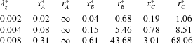
-vortex region of figure 4. The dimensional values summarized in table 1 demonstrate that the three critical points of the neutral curve could be studied experimentally by adjusting the radius of curvature and the characteristics of the free-stream disturbance.
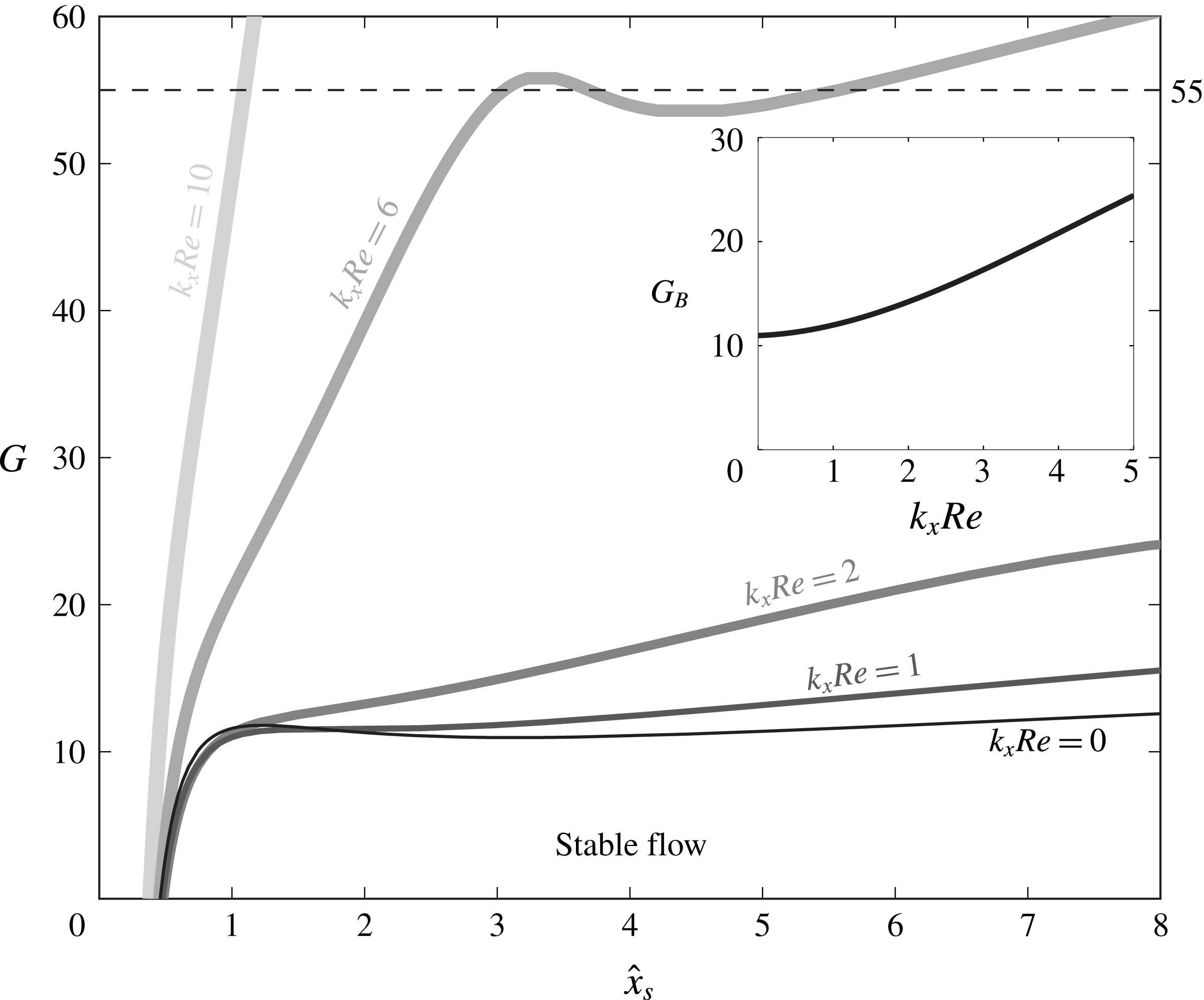
Neutral stability curves
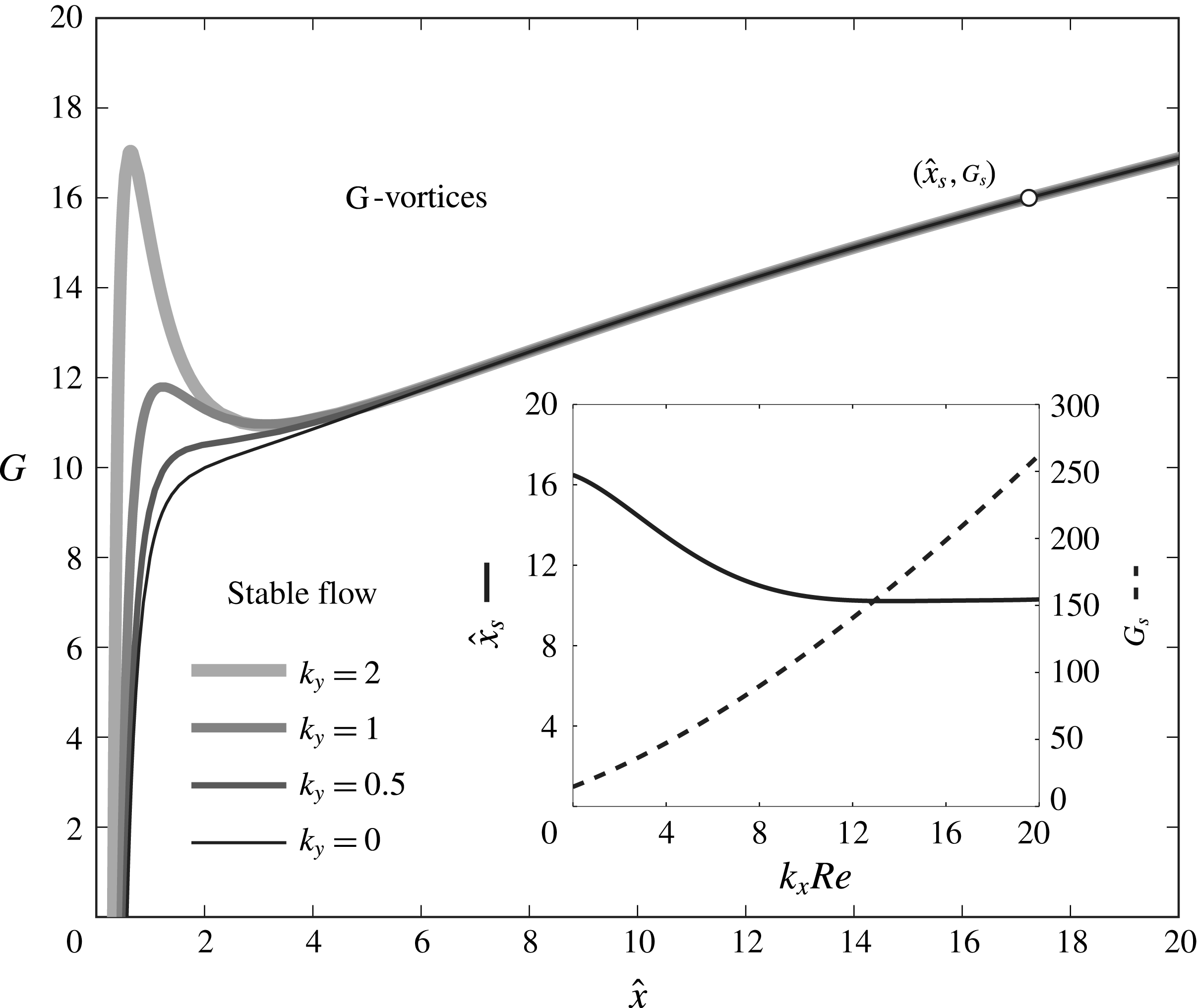
 $\unicode[STIX]{x1D70D}=0$
for
 $k_{y}=1$
and different values of the frequency
 $k_{x}Re$
. Inset: variation of the critical Görtler number
 $G_{B}$
as a function of
 $k_{x}Re$
for
 $k_{y}=1$
.

Physical locations in metres of the critical stability points for
 $k_{x}Re=0$
and
 $k_{y}=2$
, estimated from the experimental work by Boiko et al. (Reference Boiko, Ivanov, Kachanov and Mischenko2010).

3.2.2 Effect of frequency and wavelength ratio
Figures 5 and 6 show the influence of the frequency parameter
 $k_{x}Re=Re\unicode[STIX]{x1D706}_{z}^{\ast }/\unicode[STIX]{x1D706}_{x}^{\ast }$
and the wavelength ratio
 $k_{y}=\unicode[STIX]{x1D706}_{z}^{\ast }/\unicode[STIX]{x1D706}_{y}^{\ast }$
, respectively, on the neutral stability curves. For all cases, the
 $\hat{x}_{\text{K}}$
lines overlap for most Görtler numbers (not shown) and, sufficiently downstream, the neutral curves become independent of the initial conditions that are herein linked to the free-stream disturbances. Figure 5 shows that the stability region expands significantly as the frequency increases for free-stream disturbances with equal transverse wavelengths
 $\unicode[STIX]{x1D706}_{z}^{\ast }$
and
 $\unicode[STIX]{x1D706}_{y}^{\ast }$
(
 $k_{y}=1$
). Boundary layer perturbations generated by steady free-stream disturbances are therefore the most likely to turn into Görtler vortices through inviscid instability. When
 $k_{x}Re>2$
, there is a range of Görtler numbers for which the boundary layer becomes unstable again after an initial decay of Görtler vortices and before entering the permanent stable region. This scenario is shown in figure 5 for
 $k_{x}Re=6$
and
 $G=55$
. For higher frequencies, this phenomenon is even more accentuated as it occurs for a larger range of Görtler numbers. However, we focus on low-frequency disturbances as these are the most unstable and are fully consistent with our asymptotic framework, which is based on
 $k_{x}\ll 1$
.
It is also important to estimate whether TS waves may be excited by leading-edge receptivity mechanisms over flat plates (Goldstein Reference Goldstein1983; Ricco & Wu Reference Ricco and Wu2007) in the low-frequency scenario proper of the neutral curves studied herein. For the laboratory conditions of Boiko et al. (Reference Boiko, Ivanov, Kachanov and Mischenko2010) and the flat-plate case, via an in-house spatial stability code (Ricco Reference Ricco2009) we computed the neutral locations
 $\hat{x}$
downstream of which three-dimensional time-periodic TS waves grow spatially. It is sufficient to study the case at the highest frequency,
 $k_{x}Re=10$
, because the neutral stability point moves downstream as the frequency decreases. By employing the Squire transformation (Squire Reference Squire1933), which is valid for neutral conditions in the spatial stability case, we find that for our characteristic spanwise wavenumbers,
 $2\unicode[STIX]{x03C0}\unicode[STIX]{x1D6FF}^{\ast }/\unicode[STIX]{x1D706}_{z}^{\ast }\approx 2.5$
, where
 $\unicode[STIX]{x1D6FF}^{\ast }$
is the displacement thickness, three-dimensional TS waves are always stable. Three-dimensional TS waves would start growing only for
 $2\unicode[STIX]{x03C0}\unicode[STIX]{x1D6FF}^{\ast }/\unicode[STIX]{x1D706}_{z}^{\ast }$
smaller than approximately 0.08, which corresponds to very large spanwise wavelengths, i.e., larger than approximately 0.4 m.
At higher frequencies, the TS waves start amplifying at smaller
 $\hat{x}$
, but
 $k_{x}Re$
becomes too large and therefore our assumptions of low frequency and streamwise-elongated perturbations do not hold. The streamwise pressure gradient and the streamwise viscous effects of the perturbations come into play and the full linearized Navier–Stokes equations must be solved or some other asymptotic formalism, such as triple-deck theory, must be adopted. Boiko et al. (Reference Boiko, Ivanov, Kachanov and Mischenko2010) indeed included these streamwise effects in their equations and computed the TS waves, but did not account for the receptivity to external disturbances, a key ingredient in the analysis of Wu et al. (Reference Wu, Zhao and Luo2011) and in our study.
The inset of figure 5 shows the increase of the critical Görtler number
 $G_{B}$
with
 $k_{x}Re$
. Results for different
 $k_{y}$
are not shown as they overlap on the same curve due to
 $G_{B}$
being near the location where the neutral curves are independent of
 $k_{y}$
.
Neutral stability curves
 $\unicode[STIX]{x1D70D}=0$
for different values of the wall-normal wavenumber
 $k_{y}$
and
 $k_{x}Re=0$
. Inset: streamwise location
 $\hat{x}_{s}$
where the neutral curve becomes independent on
 $k_{y}$
and the corresponding Görtler number
 $G_{s}$
for different frequencies
 $k_{x}Re$
.

Figure 6 shows the influence of the wall-normal wavenumber
 $k_{y}$
for
 $k_{x}Re=0$
. The most critical scenario is for
 $k_{y}=0$
. As
 $k_{y}$
increases, i.e., as
 $\unicode[STIX]{x1D706}_{z}^{\ast }$
becomes progressively larger than
 $\unicode[STIX]{x1D706}_{y}^{\ast }$
, stability increases near the leading edge for both steady and unsteady flows, whereas the neutral curve becomes independent of
 $k_{y}$
downstream of a location
 $\hat{x}_{s}$
, defined as the
 $\hat{x}$
location where the neutral points at different
 $k_{y}$
remain within a range
 $\unicode[STIX]{x0394}\hat{x}<0.0005$
. This is in agreement with the results of Hall (Reference Hall1990) at large
 $\hat{x}$
locations. The streamwise location
 $\hat{x}_{s}$
is shown as a function of
 $k_{x}Re$
in the inset of figure 6. As the frequency increases,
 $\hat{x}_{s}$
decreases and it becomes nearly independent of the frequency for
 $k_{x}Re>10$
. The Görtler number
 $G_{s}$
associated with
 $\hat{x}_{s}$
increases monotonically with
 $k_{x}Re$
. Based on the experimental conditions of Boiko et al. (Reference Boiko, Ivanov, Kachanov and Mischenko2010),
 $\hat{x}_{s}=10$
corresponds to
 $x^{\ast }\approx 22~\text{m}$
, which means that the independence of the neutral curves on
 $k_{y}$
is not reached in realistic scenarios. As
 $k_{y}$
only occurs in the free-stream boundary conditions at leading order, this further confirms the crucial importance of solving the receptivity problem, i.e., of precisely specifying the free-stream disturbance, for the correct description of the Görtler-flow dynamics.
3.3 Receptivity coefficient
It is of practical interest to investigate the role that the outer disturbances play on the boundary layer perturbations through a receptivity coefficient
 $A$
, defined as follows. Following (Wu et al.
Reference Wu, Zhao and Luo2011, (3.1)), we first introduce the eigenvalue solution (EV) in the form
 $$\begin{eqnarray}\bar{u}_{e}(\hat{x},\unicode[STIX]{x1D702})=\widetilde{u}_{e}(\unicode[STIX]{x1D702})\;\text{exp}\left[\int _{\hat{x}_{M}}^{\hat{x}}\unicode[STIX]{x1D70E}_{EV,Re}(x)\,\text{d}x\right],\end{eqnarray}$$
where
 $\unicode[STIX]{x1D70E}_{EV}(\hat{x})$
is a complex number, whose real part
 $\unicode[STIX]{x1D70E}_{EV,Re}(\hat{x})\equiv \text{Re}\{\unicode[STIX]{x1D70E}_{EV}(\hat{x})\}$
is the local growth rate, and
 $\hat{x}_{M}$
is a streamwise location where the solution follows the modal form. Taking the absolute value and normalizing the eigenfunction
 $\widetilde{u}_{e}$
by its maximum value along
 $\unicode[STIX]{x1D702}$
we find
 $$\begin{eqnarray}|\bar{u}_{e}(\hat{x},\unicode[STIX]{x1D702})|=A\;\frac{|\widetilde{u}_{e}(\unicode[STIX]{x1D702})|}{|\widetilde{u}_{e}(\unicode[STIX]{x1D702})|_{max}}\;\text{exp}\left[\int _{\hat{x}_{M}}^{\hat{x}}\unicode[STIX]{x1D70E}_{EV,Re}(x)\,\text{d}x\right],\end{eqnarray}$$
where
 $A$
is undetermined because the eigenfunction is only obtained to within an undefined constant. If we only consider the maximum value along
 $\unicode[STIX]{x1D702}$
, (3.2) simplifies to
 $$\begin{eqnarray}|\bar{u}_{e}(\hat{x})|_{max}=A\;\text{exp}\left[\int _{\hat{x}_{M}}^{\hat{x}}\unicode[STIX]{x1D70E}_{EV,Re}(x)\,\text{d}x\right].\end{eqnarray}$$
We then express the amplitude of the LUBR streamwise velocity
 $\bar{u}(\hat{x},\unicode[STIX]{x1D702})$
in an analogous form,
 $$\begin{eqnarray}|\bar{u}(\hat{x})|_{max}=A(\hat{x})\;\text{exp}\left[\int _{\hat{x}_{M}}^{\hat{x}}\unicode[STIX]{x1D70E}_{EV,Re}(x)\,\text{d}x\right],\end{eqnarray}$$
which defines the streamwise-dependent receptivity coefficient
 $A(\hat{x})$
implicitly. Equation (3.4) shows that from
 $A(\hat{x})$
and the EV solution it is possible to obtain the LUBR maximum amplitude of the streamwise velocity perturbation inside the boundary layer and therefore investigate the influence of the outer disturbances in terms of
 $k_{y}$
,
 $k_{x}Re$
and
 $G$
. We note that
 $A=A(\hat{x})$
is streamwise-dependent. It would be constant only if the growth rate computed from the boundary region solution,
 $|\bar{u}^{\prime }(\hat{x})|_{max}/|\bar{u}(\hat{x})|_{max}$
, were equal to
 $\unicode[STIX]{x1D70E}_{EV,Re}(\hat{x})$
, i.e., the streamwise dependence of the LUBR solution were completely predicted by the EV growth rate. This is, however, not the case because the EV solution does not take into account the influence of the oncoming flow.
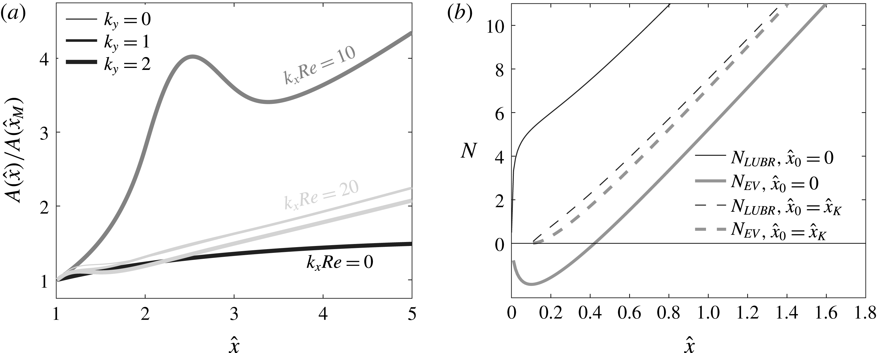
Influence of frequency
 $k_{x}Re$
and
 $k_{y}$
on the normalized coefficient
 $A(\hat{x})$
for
 $G=300$
(a). Amplification factor
 $N$
based on the LUBR and EV approaches calculated at different starting locations for
 $k_{x}Re=0$
,
 $G=300$
,
 $k_{y}=1$
(b).

Figure 7(a) shows the influence of
 $k_{x}Re$
and
 $k_{y}$
on
 $A(\hat{x})$
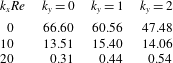
, normalized by the values of
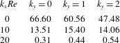
 $A(\hat{x}_{M})$
found in table 2. The boundary layer perturbations are more influenced by the oncoming flow conditions as the frequency increases. The receptivity coefficient is nearly constant only for
 $k_{x}Re=0$
and large
 $\hat{x}$
. The intense effect of the frequency was also noted by Boiko et al. (Reference Boiko, Ivanov, Kachanov, Mischenko and Nechepurenko2017) through a receptivity coefficient defined by optimal disturbances. As the frequency increases the effect of
 $k_{y}$
increases as well. As
 $G$
increases, the influence of
 $k_{y}$
decreases and
 $A(\hat{x})$
becomes more independent of
 $\hat{x}$
, i.e., the solution
 $|\bar{u}(\hat{x})|_{max}$
evolves closer to a pure exponential form in a wider
 $\hat{x}$
-range. This is expected because the EV exponential solution (3.1) is valid in the asymptotic limit
 $G\gg 1$
.
Receptivity coefficient
 $A(\hat{x}_{M})$
for
 $G=300$
.
3.4
 $N$
-factor

We close this paper with a comment on the effect of free-stream disturbance on the amplification factor (or
 $N$
-factor) widely used in transition-prediction studies (Van Ingen Reference Van Ingen1956; Jaffe et al.
Reference Jaffe, Okamura and Smith1970) and defined as
 $$\begin{eqnarray}N(\hat{x})\equiv \int _{\hat{x}_{0}}^{\hat{x}}\unicode[STIX]{x1D70E}(x)\,\text{d}x,\end{eqnarray}$$
where
 $\unicode[STIX]{x1D70E}$
is the growth rate computed through either the LUBR or the EV solution, leading to
 $N_{LUBR}$
and
 $N_{EV}$
, respectively. Engineers have used the value
 $N=9$
to predict the streamwise location where transition occurs, but, as figure 7(b) shows, this approach is ambiguous. Not only does the
 $N$
-factor calculated through the EV solution significantly underestimate the
 $N$
-factor at fixed
 $\hat{x}$
computed through the LUBR solution, but there is also a strong dependence on the starting location where the
 $N$
-factor is computed. The disagreement between
 $N_{LUBR}$
and
 $N_{EV}$
increases significantly when the
 $N$
-factor is computed from
 $\hat{x}_{0}=0$
. This is due to the rapid initial growth of
 $\text{K}$
-vortices which the simplified EV approach is unable to capture. The agreement between these two solutions improves if the
 $N$
-factor is computed from
 $\hat{x}_{0}=\hat{x}_{\text{K}}$
(the location where the Görtler vortices start amplifying) or if
 $\hat{x}_{0}$
is in the region of modal growth. However, the definition of
 $\hat{x}_{0}$
still remains arbitrary and one has to carefully verify the conditions associated with the calculation of the
 $N$
-factor when using it for transition prediction. The rigorous mathematical formulation of the Görtler flow based on the receptivity due to free-stream disturbances does not help improve the reliability of the
 $N$
-factor approach for the transition prediction, in line with previous works revealing problems with this methodology (Smith Reference Smith1955; Malik et al.
Reference Malik, Li, Choudhari and Chang1999; Boiko et al.
Reference Boiko, Ivanov, Kachanov, Mischenko and Nechepurenko2017).
Our work on the neutral curve can be further generalized by taking into account the influence of convex curvature and by introducing the nonlinear effects studied by Xu, Zhang & Wu (Reference Xu, Zhang and Wu2017), therefore relaxing the assumption of small-amplitude perturbations (Ustinov Reference Ustinov2013).
Acknowledgement
We wish to acknowledge the support of the US Air Force through the AFOSR grant FA9550-15-1-0248. We would also like to thank Dr M. E. Goldstein, Professor A.V. Boiko and Drs E. Marensi, P. D. Hicks, C. Alvarenga, and E. Zincone for providing insightful comments on a preliminary version of the paper. We also thank the referees for their useful comments.