


1. Introduction
Central banks need to assess the risks of extreme events, such as very poor (or very good) expected economic growth and price increases (or decreases) to conduct policy. As a consequence, the academic literature on growth-at-risk (Adrian et al. Reference Adrian, Boyarchenko and Giannone2019) and inflation-at-risk (Lopez-Salido and Loria, Reference Lopez-Salido and Loria2024), which seeks to quantify the probabilities of such extremes has expanded significantly in recent years. In this paper, I study how US monetary policy shocks affect these probabilities by characterizing the full conditional distributions of GDP growth and inflation, rather than individual quantiles alone (Schröder, Reference Schröder2024). To this end, the present paper makes the following contributions. First, I address an important hurdle in the at-risk literature—the selection of the variables that constitute the information set (Plagborg-Møller et al. Reference Plagborg-Møller, Reichlin, Ricco and Hasenzagl2020). I approach this issue by extracting a set of factors from the FRED-QD database, which capture broad information on industrial production, employment, financial markets, and other segments of macroeconomic importance and therefore constitute a more comprehensive information set than that obtained using single factors such as the commonly used National Financial Conditions Index (NFCI) (Adrian et al. Reference Adrian, Boyarchenko and Giannone2019). Equipped with these factors, I rely on the quantile regression methodology of Adrian et al. (Reference Adrian, Boyarchenko and Giannone2019) and fit individual quantiles of the annual percentage changes in GDP and the PCE price index (PCECTPI). A second challenge within the at-risk framework is the characterization of the full conditional distribution of the target variable. Typically this is done using the skew-t distribution of Azzalini and Capitanio (Reference Azzalini and Capitanio2003). However, this particular distribution does not allow for multimodality. Instead, I fit kernel distributions to obtain fully flexible conditional distributions. Finally, I add dynamic causal inference to the model building on the work of Forni et al. (Reference Forni, Gambetti and Sala2025) and Adrian et al. (Reference Adrian, Boyarchenko and Giannone2021), by combining the fitted distributions with the impulse response functions (IRFs) implied by a dynamic factor model.
I document the following new findings: contrary to much of the established literature, the left tail of expected GDP growth is not significantly more volatile than the right tail, when accounting for broad macroeconomic information through factors extracted from a large macroeconomic database, suggesting that variable selection matters for this result. Moreover, multimodality of the predicted conditional distributions is the norm rather than the exception. Contractionary monetary policy shocks shift the expected GDP distribution to the left, in line with standard findings, but emphasize its two humps. Mean inflation is reduced, but a significant probability mass associated with unchanged or even increased inflation after the monetary policy shock persists. Therefore, the inflation distribution spreads out. Hence, the shock induces changes in the economy which lead to expected reductions in inflation, but tail risks can remain.
Much of the existing research in this area has focused on determining the best set of conditioning variables to accurately describe the expected distributions of inflation and growth, for the purpose of in-sample analysis (see Giglio et al. (Reference Giglio, Kelly and Pruitt2016), Adrian et al. (Reference Adrian, Boyarchenko and Giannone2019), Adrian et al. (Reference Adrian, Grinberg, Liang, Malik and Yu2022), and Lopez-Salido and Loria (Reference Lopez-Salido and Loria2024)) or out-of-sample nowcasting and forecasting (see Ghysels et al. (Reference Ghysels, Iania and Striaukas.2018), Plagborg-Møller et al. (Reference Plagborg-Møller, Reichlin, Ricco and Hasenzagl2020), Adams et al. (Reference Adams, Adrian, Boyarchenko and Giannone2021), and Carriero et al. (Reference Carriero, Clark and Marcellino2025). Some important contributions to the causal analysis of macroeconomic shocks include Duprey and Ueberfeldt (Reference Duprey and Ueberfeldt2020), Boire et al. (Reference Boire, Duprey and Ueberfeldt2021), Loria et al. (Reference Loria, Matthes and Zhang2023), Forni et al. (Reference Forni, Gambetti, Maffei-Faccioli and Sala2024), and Forni et al. (Reference Forni, Gambetti and Sala2025). Chavleishvili and Manganelli (Reference Chavleishvili and Manganelli2024) offer a combined framework for forecasting and structural inference. The contribution of this paper with respect to this literature consists in the combination of the quantile regression framework with a factor model, which has been shown to resolve important empirical puzzles in the causal analysis of monetary policy shocks (see Forni and Gambetti (Reference Forni and Gambetti2010) and Kerssenfischer (Reference Kerssenfischer2019)) and can produce good forecasting results for the mean (Stock and Watson, Reference Stock and Watson2002) and reasonable out-of-sample results for conditional quantiles (Carriero et al. Reference Carriero, Clark and Marcellino2025).
In a study close to this one, Loria et al. (Reference Loria, Matthes and Zhang2023) analyze how different macroeconomic shocks—monetary policy included— affect the conditional quantiles of GDP growth using the quantile regression model of Adrian et al. (Reference Adrian, Boyarchenko and Giannone2019) as a case study. Their study differs from this paper in the following ways: first, they use the conditional quantiles of Adrian et al. (Reference Adrian, Boyarchenko and Giannone2019), whereas I construct new forecasted quantiles using a factor approach. Second, they use local projections to gauge the effect of the monetary policy shock, whereas I use a combination of quantile regression and a dynamic factor model. Forni et al. (Reference Forni, Gambetti, Maffei-Faccioli and Sala2024) use a quantile regression–SVAR framework to study the effects of monetary policy and financial shocks on the US economy. They find that large monetary expansions are needed to counteract bad financial shocks with high costs in terms of inflation risk. Their study differs from mine, as the authors use an SVAR instead of a DFM and rely on monthly instead of quarterly data. Moreover, they focus on specific quantiles rather than the full conditional distribution of the target variables.
The rest of this paper is organized as follows: Section 2 presents how the DFM is combined with quantile regressions to obtain quantile IRFs. Section 3 describes the data set, transformations, and model specification. Section 4 presents the results. Section 5 offers a discussion of the results and Section 6 concludes.
2. Econometric approach
The main relationship that I use in this paper is an extension of the QR-SVAR of Forni et al. (Reference Forni, Gambetti and Sala2025) and is given by
 \begin{equation} Q_{t+h,\tau } = \beta _\tau (L)Wf_t = \beta _\tau (L)WH(L)u_t \end{equation}
 $Q_{t+h,\tau }$
stands for the
 $h$
period ahead prediction of the conditional quantile of a variable of interest. In this paper, the variables of interest are GDP growth and inflation.
 $\beta _\tau (L)$
is a polynomial in the lag-operator
 $L$
of the coefficients
 $\beta _\tau$
obtained from a quantile regression of the variable of interest on a set of predictors, selected by the matrix
 $W$
. The set of predictors is made up of the static factors
 $f_t$
that are extracted from a large macroeconomic data set. The factors are assumed to follow an invertible VAR relationship and therefore, can be cast into the corresponding moving average (MA) representation. The structural MA representation is then given by
 $H(L)u_t$
, where
 $H(L)$
are the structural impulse responses and
 $u_t$
are the structural shocks. The monetary policy shock is identified using the dynamic factor model approach of Forni and Gambetti (Reference Forni and Gambetti2010). This relationship exploits the high information content in the static factors as potentially useful predictors for the conditional quantiles of the variables of interest and simultaneously makes use of large information approach to the identification of monetary policy shocks that has been shown to perform similarly to other accepted methods such as high-frequency identification (Kerssenfischer, Reference Kerssenfischer2019).
2.1 The dynamic factor model
The methodology used to estimate factors and identify the structural shocks is based on the dynamic factor model of Forni and Gambetti (Reference Forni and Gambetti2010). Given a large data set of macroeconomic variables with cross-sectional dimension
 $N$
and time span
 $T$
, the following relationship is assumed to be present in the set:
 \begin{equation} x_{it} = \chi _{it} + \xi _{it} \end{equation}
Here,
 $x_{it}$
is one of the
 $N$
variables in the data set at time
 $t$
.
 $\chi _{it}$
is the common component and
 $\xi _{it}$
is the idiosyncratic component. Common and idiosyncratic components are assumed to be orthogonal. The idiosyncratic components of different variables are allowed to be mildly correlated. The latter implies that the factor model is approximate and not exact (Bai and Ng, Reference Bai and Ng2002). In addition, I assume that the common component
 $\chi _{it}$
is driven by
 $r$
common factors
 $f_t$
. The importance each of these
 $r$
factors has for the common component is captured by a vector of loadings
 $a_i$
. Hence,
 \begin{equation} \chi _{it} = a_i f_t \end{equation}
Next, I assume that the common factors follow a VAR which is assumed to be invertible and given by
 \begin{equation} D(L)f_t = \epsilon _t \end{equation}
with
 $D(L)$
a matrix polynomial of coefficients in the lag operator
 $L$
and
 $\epsilon _t$
a vector of zero-mean reduced form shocks. As in Forni and Gambetti (Reference Forni and Gambetti2010), the number of structural shocks
 $u_t$
driving the common factors
 $f_t$
need not be equal to the number of factors
 $r$
. Instead, it is possible that the number of deep shocks
 $q$
is smaller than the number of factors, that is,
 $q\leq r$
. This is captured by a rotation
 $R$
such that
 $\epsilon _t = R u_t$
.
 \begin{equation} D(L)f_t = R u_t \end{equation}
The vector
 $u_t$
is assumed to be a vector white noise process and holds the deep shocks in the economy. One of these shocks is assumed to be a monetary policy shock which can be identified in the following way.
2.2 Identification of the monetary policy shock
The identification strategy for the monetary policy shocks builds on the work of Bernanke et al. (Reference Bernanke, Boivin and Eliasz2005) who show that a simple recursive strategy can successfully eliminate the price puzzle that frequently occurs in monetary SVAR analysis with small systems, as long as additional information through factors is incorporated. For this purpose the authors propose the factor-augmented VAR (FAVAR), which includes both economic variables (notably the Federal Funds Rate) and factors extracted from a large data set. Forni and Gambetti (Reference Forni and Gambetti2010) then extend the setting to the DFM of Forni et al. (Reference Forni, Giannone, Lippi and Reichlin2009) to use an information-rich statistical model to identify monetary policy shocks. They simultaneously resolve the price and the delayed-overshooting puzzles which occur frequently in smaller, recursively identified models.
Beginning from equation (5), invertibility provides that the factors can be written as
 \begin{equation} f_t = D(L)^{-1}Ru_t \end{equation}
For any orthogonal matrix
 $H$
equation (6) can be rewritten as
 \begin{equation} f_t = D(L)^{-1}RH'Hu_t=D(L)^{-1}SHu_t=S(L)Hu_t = H(L)u_t \end{equation}
which is the relation used in model (1) with
 $S=RH'$
,
 $S(L)=D(L)^{-1}S$
, and
 $H(L) = S(L)H$
. Similar to the SVAR literature, the model is not identified without further assumptions on the matrix
 $H$
. The objective is to identify a monetary policy shock in the same way that traditional recursive SVARs, as for example, Christiano et al. (Reference Christiano, Eichenbaum and Evans1999) do—by imposing that the monetary policy shock does not contemporaneously affect slow moving variables such as GDP or prices, but can contemporaneously affect financial variables and interest rates. However, it is not possible to impose such restrictions on the factors
 $f_t$
directly as they lack a concrete interpretation. Hence, I impose the restriction with a view to the common component
 $\chi _{it}$
of the macro panel instead.
Using equations (7) and (3), we obtain the structural IRFs of the common components
 $b_i(L)$
from
 \begin{equation} \chi _{it} = a_iD(L)^{-1}RH'Hu_t=a_iS(L)v_t=c_i(L)v_t=c_i(L)Hu_t=b_i(L)u_t \end{equation}
where
 $c_i(L) = a_iS(L)$
and
 $b_i(L) = c_i(L)H$
. Therefore, the IRFs in
 $b_i(L)$
have to fulfill the identifying assumptions. In the Cholesky case preferred in this paper, this is achieved by selecting exactly
 $m=q$
variables from
 $x_{it}$
and ordering them according to the assumed recursive structure. Since,
 \begin{equation} B_m(L) = C_m(L)H \end{equation}
the restrictions are imposed contemporaneously by setting
 \begin{equation} H = C_m(0)^{-1}G_m \end{equation}
where
 $C_m(0)^{-1}$
is the inverse of the non-structural IRF on impact and
 $G_m$
is the lower triangular Cholesky factor of
 $C_m(0)C_m(0)'$
.
The recent literature has brought forward many innovations in the field of monetary policy shock identification, most prominently through the use of high-frequency proxies (Gertler and Karadi, Reference Gertler and Karadi2015; Miranda-Agrippino and Ricco, Reference Miranda-Agrippino and Ricco2021). This approach is predominantly applied in monthly SVAR analysis. Miescu and Mumtaz (Reference Miescu and Mumtaz2019) and Brignone et al. (Reference Brignone, Franconi and Mazzali2023) provide first extensions to the FAVAR/DFM environment. I check robustness of all results by using the proxy variable of Bauer and Swanson (Reference Bauer and Swanson2023) as an external instrument. The results for this are close to the recursive approach and reported in the Online Appendix.
2.3 Quantile regressions
The second step consists in running a predictive regression of the variables of interest—GDP growth and inflation—on the respective sets of predictors, the factors in model (1). While OLS regressions are concerned with the mean response of the dependent variable to changes in different explanatory variables, quantile regression (Koenker and Bassett, Reference Koenker and Bassett1978) is concerned with the median and other quantiles of the distribution of the dependent variable. In this sense, it is more robust to potential outliers that may distort the mean and, in addition, allows the study of the drivers of more extreme outcomes of GDP growth and inflation, such as
 $\tau =0.05,0.1,0.9,0.95$
, which are the common quantiles studied in the literature on “growth-at-risk”.
Koenker (Reference Koenker2005) shows that
 $\hat {\beta }_\tau$
solves the minimization problem of the conditional sample quantile function
 $Q_{t,\tau }$
as in
 \begin{equation} \min _{\beta \in \mathbb{R}^p} \sum _{i=1}^n\rho _\tau (y_i-x_i'\beta ) \end{equation}
where
 $p$
is the number of regressors,
 $\rho$
is the loss function
 $\rho _\tau (u) = u(\tau - \unicode {x1D7D9}(u\lt 0))$
with
 $u_i = y_i-x_i'\beta$
and
 $y_i$
being the dependent variable. This is a linear programming problem that can be solved using simplex methods. Hence, the quantile relationship I use is given by
 \begin{equation} Q_{t+h,\tau } = \beta _\tau (L)Wf_t \end{equation}
Throughout the paper, the generic issue of “quantile-crossing” is dealt with using the methodology of Chernozhukov et al. (Reference Chernozhukov, Fernández-Val and Galichon2010).
2.4 Combining quantile regression and dynamic factor model
From the estimated coefficients
 $\widehat {\beta _\tau (L)}$
and given the selection of regressors
 $Wf_t$
I can pin down the IRFs of the conditional quantiles of GDP growth and inflation for a monetary policy shock. This allows an assessment of whether the uncertainty around future economic conditions is reduced, increased or not affected by policy action. Moreover, since I study the three quantiles individually it may be that downside risk (as measured by Q05) is affected differently than upside risk (as measured by Q95) by the shock.
The IRFs are given by
 \begin{equation} IRF_\tau ^{GDP} = \widehat {{\beta _\tau ^{GDP}}(L)}W_{GDP}H(L) \end{equation}
 \begin{equation} IRF_\tau ^\pi = \widehat {{\beta _\tau ^\pi }(L)}W_{\pi }H(L) \end{equation}
Since I include all factors as regressors, the matrices
 $W$
are identity matrices in both cases. The matrix polynomial
 $H(L)$
is given by
 $D(L)^{-1}SH$
as described in equation (7). The above expressions can also be used to carry out an analysis of the forecast error variance of the quantiles and decompose the conditional time series for each quantile into the contributions coming from the monetary policy shock and other, undetermined factors.
2.5 Density impulse responses
In addition to the responses of individual conditional quantiles, I compute the change in the full conditional density after the monetary policy shock. I start by fixing a baseline distribution at the time mean of the factors
 $\bar {f}$
. Together with the estimated quantile coefficients
 $\widehat {\beta }_\tau$
, I obtain predicted quantiles
 $\widehat {Q}_{baseline,\tau }$
over a discrete grid of quantiles
 $\tau \ \in \{0.01, 0.02, \ldots , 0.99\}$
. Next, I construct the conditional density non-parametrically via adaptive kernel smoothing (Portnoy and Koenker, Reference Portnoy and Koenker1989) using a Gaussian kernel
 $K(\!\cdot \!)$
. The approximated density for the random variable of choice
 $z$
is denoted by
 $\hat {g}(z)$
.
 \begin{equation} \hat g(z) = \sum _i \Delta \tau _i \cdot \frac {1}{h(\tau _i)} \; K\!\left ( \frac {z - Q(\tau _i)}{h(\tau _i)} \right ) \end{equation}
 $\Delta$
denotes the difference
 $\tau _i-\tau _{i-1}$
. The adaptive kernel bandwidth
 $h(\!\cdot \!)$
uses the pilot density
 $\widehat {g}_0$
constructed from a rule-of-thumb (
 $RoT$
) bandwidth,
 $h^{RoT}$
fixed using Silverman (Reference Silverman1986) (p. 48). The parameter
 $\alpha$
controls the sensitivity to the pilot density and is set to 0.5 throughout, a standard value (see Portnoy and Koenker (Reference Portnoy and Koenker1989) p. 374).
 \begin{align} h &= h^{RoT} \left ( \frac {\widehat {g}_0\big (\widehat {Q}_{\tau }\big )}{m} \right )^{-\alpha } \end{align}
 \begin{align} \log m &= \sum _i \Delta \tau _i \log \widehat {g}_0 \end{align}
This produces a baseline density when the factors are at their sample average, called
 $g^{baseline}$
. Next, I compute a perturbation of the baseline factors
 $\bar {f} + H(L)u_t^{mp}$
for
 $j = 0, 1,\ldots ,40$
periods using the estimated impulse responses
 $H(L)$
. For each horizon and each quantile, the fitted conditional quantile is computed using
 $\beta _\tau$
and the adaptive kernel smoothing is applied again. As a consequence of this approach, non-linearity in
 $u_t$
enters in two ways: through the smoothing kernel
 $K(\!\cdot \!)$
and through the adaptive bandwidth
 $h(\!\cdot \!)$
. This produces a sequence of densities
 $\left \{ g^{j} \right \}_{j=1}^{40}$
which can be compared with the baseline density in a similar way to Chang et al. (Reference Chang, Chen and Schorfheide2024) by computing the difference between the baseline and the perturbed density.
3. Data and model specification
The data set for the factor model is the collection of US quarterly macroeconomic variables of McCracken and Ng (Reference McCracken and Ng2020), which is gathered by FRED of the Federal Reserve Bank of St. Louis. The data set contains 248 variables from Q1:1959 to Q4:2023. Variables are transformed to induce stationarity. Price series are kept in single differences since the quantile regression outcome for inflation-at-risk is also single differenced. The Online Appendix reports all variables that are included, their transformations and the variation explained by the static factors.
The data set contains missing values and outliers. Outliers are problematic for principal components analysis (PCA) and are dealt with as suggested in McCracken and Ng (Reference McCracken and Ng2020) by omitting values whose difference from the median is larger than ten times the interquartile range. These outliers are replaced by missing values. To deal with the missing values I use the expectation maximization algorithm of McCracken and Ng (Reference McCracken and Ng2020). I tweak their procedure by using the selection criterion of Alessi et al. (Reference Alessi, Barigozzi and Capasso2010) which is a refined version of the criterion of Bai and Ng (Reference Bai and Ng2002) to determine the optimal number of factors at each iteration. The optimal number of static factors to include in
 $f_t$
is determined to be between
 $r=8$
and
 $r=15$
. For parsimony, I prefer the lower of the two as my benchmark and check robustness of the results against the upper bound. Factors are estimated using the principal component estimator.
In a second step, I determine the lag length to be used in the VAR for the factors using the Hannan-Quinn, Schwarz, and Akaike information criteria (AIC). These suggest
 $p=1$
(HQ, SC) and
 $p=3$
(AIC). Again, for parsimony, I choose
 $p=1$
and check robustness of the results for
 $p=3$
. Finally, the number of dynamic factors or primitive shocks is determined using the criterion of Bai and Ng (Reference Bai and Ng2007), which suggests to set
 $q=4$
when
 $r=8$
. For the purpose of identification
 $m=q=4$
identifying variables are required. I use the variables for real GDP (GDPC1), the PCECTPI, the Federal Funds Rate (FEDFUNDS), replaced by the shadow rate (Wu and Xia, Reference Wu and Xia2016) between Q4:2008 and Q1:2022, and the USD-CHF exchange rate (EXSZUS), in that order. This setup is similar to Forni and Gambetti (Reference Forni and Gambetti2010) and implies that the monetary policy shock is the third one in
 $u_t$
. It does not drive GDP or prices on impact, but can contemporaneously influence the Federal Funds Rate and the exchange rate.
In the quantile regression exercise I follow Adrian et al. (Reference Adrian, Boyarchenko and Giannone2019) and set
 $\tau = 0.05, 0.5, 0.95$
to capture the tail behavior of the conditional distribution of the dependent variables real GDP growth (GDPC1) and PCE inflation (PCECTPI). Four quarter ahead growth rates (
 $h=4$
) are computed as the difference of the logs between
 $t$
and
 $t-4$
and multiplied by 100. The median is useful for comparison to the mean and to compute descriptive statistics such as the Kelley skewness of the conditional distributions implied by the estimates. The forecast horizon is
 $h=4$
quarters. For the estimation of the quantile regression part in model (1), there are
 $r=8$
static factors available as potential predictors, as well as their lags. To keep the model simple I do not include additional predictors and do not add lags to the quantile regressions. Hence, the matrix
 $W$
in equation (1) is an identity matrix and
 $\beta _\tau (L)$
is just
 $\beta _\tau$
.
4. Results
4.1 Monetary policy shock IRFs
Figure 1 shows the impulse responses of the four identifying variables to the Cholesky monetary policy shock, scaled to a 100 basis points increase in the Federal Funds Rate. The shock decreases the levels of GDP and prices and affects the exchange rate between Swiss Francs and US Dollars in line with the overshooting principle of Dornbusch (Reference Dornbusch1976). The classical “price puzzle” and “delayed-overshooting puzzle” do not obtain, and the results are in line with Cholesky-DFM results presented in Forni and Gambetti (Reference Forni and Gambetti2010) as well as Kerssenfischer (Reference Kerssenfischer2019). Notice that this can be shown to obtain regardless of using the real exchange rate or nominal one as I do (Kim et al. Reference Kim, Moon and Velasco2017).
Point estimates of the impulse responses of the identifying variables to a contractionary 100bp monetary policy shock with bootstrapped 90% confidence intervals.

4.2 Quantile regression predictions
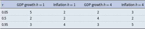
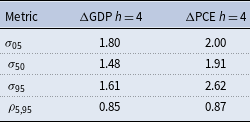
For every quantile considered here at least three of the factors are highly significant predictors, as can be seen in Table 1. Figure 3 shows the time-varying quantiles as predicted using the factor approach from equation (12) for year-on-year real GDP growth and PCE inflation. As distinct from other forecasts in the literature, the median, and Q95 predictions of GDP growth appear more volatile, while the higher volatility of Q05 that is observed in Adrian et al. (Reference Adrian, Boyarchenko and Giannone2019) and Forni et al. (Reference Forni, Gambetti and Sala2025) is also featured as shown in Table 2.
Number of significant factors by quantile. 90% significance is assessed using bootstrapped standard errors (Koenker, Reference Koenker1994)

Table 1. Long description
A table comparing GDP growth and inflation across different quantiles and time horizons. The table has four rows and four columns. The columns are labeled with different quantiles (0.05, 0.5, 0.95) and the rows are labeled with different metrics (GDP growth h = 1, Inflation h = 1, GDP growth h = 4, Inflation h = 4). Row 1: GDP growth h = 1, 5, 2, 2. Row 2: Inflation h = 1, 2, 2, 2. Row 3: GDP growth h = 4, 2, 4, 3. Row 4: Inflation h = 4, 3, 2, 5.
Standard deviations of predicted quantiles and correlation coefficient for the extreme quantiles

Table 2. Long description
A table with two columns and four rows. The columns are labeled “ΔGDP h = 4” and “ΔPCE h = 4”. The rows are labeled with different standard deviations: σ05, σ50, σ95, and ρ5,95. The values in the table are as follows: Row 1: ΔGDP h = 4, 1.80; ΔPCE h = 4, 2.00. Row 2: ΔGDP h = 4, 1.48; ΔPCE h = 4, 1.91. Row 3: ΔGDP h = 4, 1.61; ΔPCE h = 4, 2.62. Row 4: ΔGDP h = 4, 0.85; ΔPCE h = 4, 0.87.
Especially the downside growth risk increases around the recessionary periods in the mid 1970s, early 1980s, early 1990s, and 2000s as well as the Great Recession are clearly visible. However, the model predicts a very rapid recovery of downside growth risk and median risk after the 2007-2008 recessionary episode. The COVID period is not included in the quantile range at all. Moreover, the interquantile range decreases markedly with the Great Moderation as shown in Figure 4. During most periods the expected distribution of GDP growth was negatively (left) skewed which suggests a longer left tail relative to the right tail.
As for the predicted quantiles of PCE inflation, a downward trend is observable with sharp increases in the right tail in the recessions of the 1970s and 1980s but a pronounced drop in the lower tail during the Great Recession and COVID-19. The fall in the interquantile range is not as clear cut as with GDP growth, but during the period of the Great Moderation, the spread measure is less volatile up to the Great Recession. According to the non-normalized Kelley skewness, PCE inflation predictions were almost always positively (right) skewed, which suggests a longer right tail with more extremely high predictions. By a similar token, Table 2 shows that the upper tail was much more volatile than the lower tail over the considered horizon.
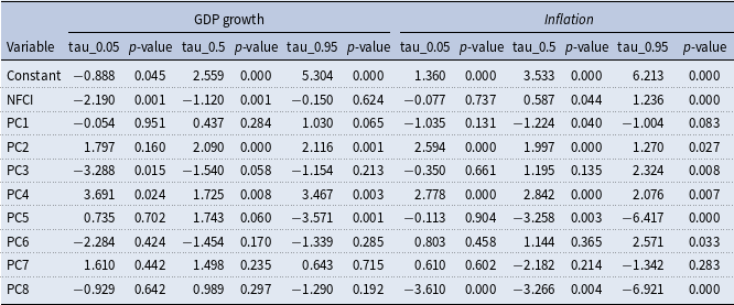
Quantile regression results for GDP growth and inflation at
 $h=4$
with NFCI and 8 FRED-QD factors

Table 3. Long description
The table presents quantile regression results for GDP growth and inflation with NFCI and 8 FRED-QD factors. It has 9 rows and 12 columns. The columns are labeled as follows: Variable, tau_0.05 p-value, tau_0.5 p-value, tau_0.95 p-value, tau_0.05 p-value, tau_0.5 p-value, tau_0.95 p-value. The rows are labeled with variables: Constant, NFCI, PC1, PC2, PC3, PC4, PC5, PC6, PC7, PC8. Each row contains values for the respective variables across different quantiles and p-values. Notable trends include significant p-values for several variables, indicating their impact on GDP growth and inflation at different quantiles.
Kelley skewness in the conditional GDP growth distribution (h = 4) from the NFCI for different information sets. Each line is the value associated only with the NFCI, but the involved coefficients are re-estimated in quantile regressions with an iteratively expanding information set.

h = 4 predicted quantiles (Top line: Q95, light gray line: Q50, bottom line: Q05) of GDP growth and PCE inflation. Red dashed line is the realized series.

Top graph is interquantile range over time (Q95–Q05), bottom graph is non-normalized Kelley skewness (Q95+Q05-2
 $\times$
Q50).

To better understand the difference between the quantile predictions based on factors and those prevalent in the literature, I perform two additional checks. First, I recompute the quantile regressions for all factors jointly with the NFCI to assess whether the role of the NFCI changes once large information is controlled for. The estimation results are presented in Table 3, which shows that the NFCI does not loose its significance for the lower tail of predicted GDP growth or the upper tail of inflation. However, importantly, at least some of the factors remain highly predictive as well. Especially the factors related to prices, credit, and long-term interest rates add information on top of the NFCI to the prediction of growth-at-risk, while almost all factors are helpful predictors of the upper tail of inflation on top of the NFCI (see the Online Appendix for details). As the goal of this paper is to analyze the response of the conditional distributions of GDP growth and inflation to monetary policy shocks, it is crucial to capture as comprehensive a set of channels for policy transmission as possible. Using factors can provide a consistent way of doing that.
Second, I gradually expand the information set in the quantile regressions by adding factors one by one to the NFCI and recomputing each time the predicted quantiles. A key contribution of Adrian et al. (Reference Adrian, Boyarchenko and Giannone2019) is the finding that the NFCI predicts downside asymmetries in the GDP growth distribution, but is less relevant for upside growth risk. These can be captured by the Kelley skewness. Based on the fitted quantiles I calculate this asymmetry indicator for each expanding information set, based solely on the contributions of the NFCI. If the asymmetry-inducing property of the NFCI is consistent, it should be more or less unchanged when additional information enters the quantile regressions. However, Figure 2 shows that the role of the NFCI for asymmetries changes substantially in the presence of additional information. When only the NFCI enters the quantile regression, the asymmetry is almost exclusively negative as in Adrian et al. (Reference Adrian, Boyarchenko and Giannone2019). Once more factors are added, the 1970s and 1980s, but also the 2020s display also right skewness entering through the NFCI. The role of the NFCI appears to settle once more than four factors are included. I consider this supporting evidence for the chosen approach, as considering the NFCI alone (together with lagged output growth) as is done, for example, in Loria et al. (Reference Loria, Matthes and Zhang2023), may lead to diverging results for the transmission of monetary policy shocks, as important channels are omitted.
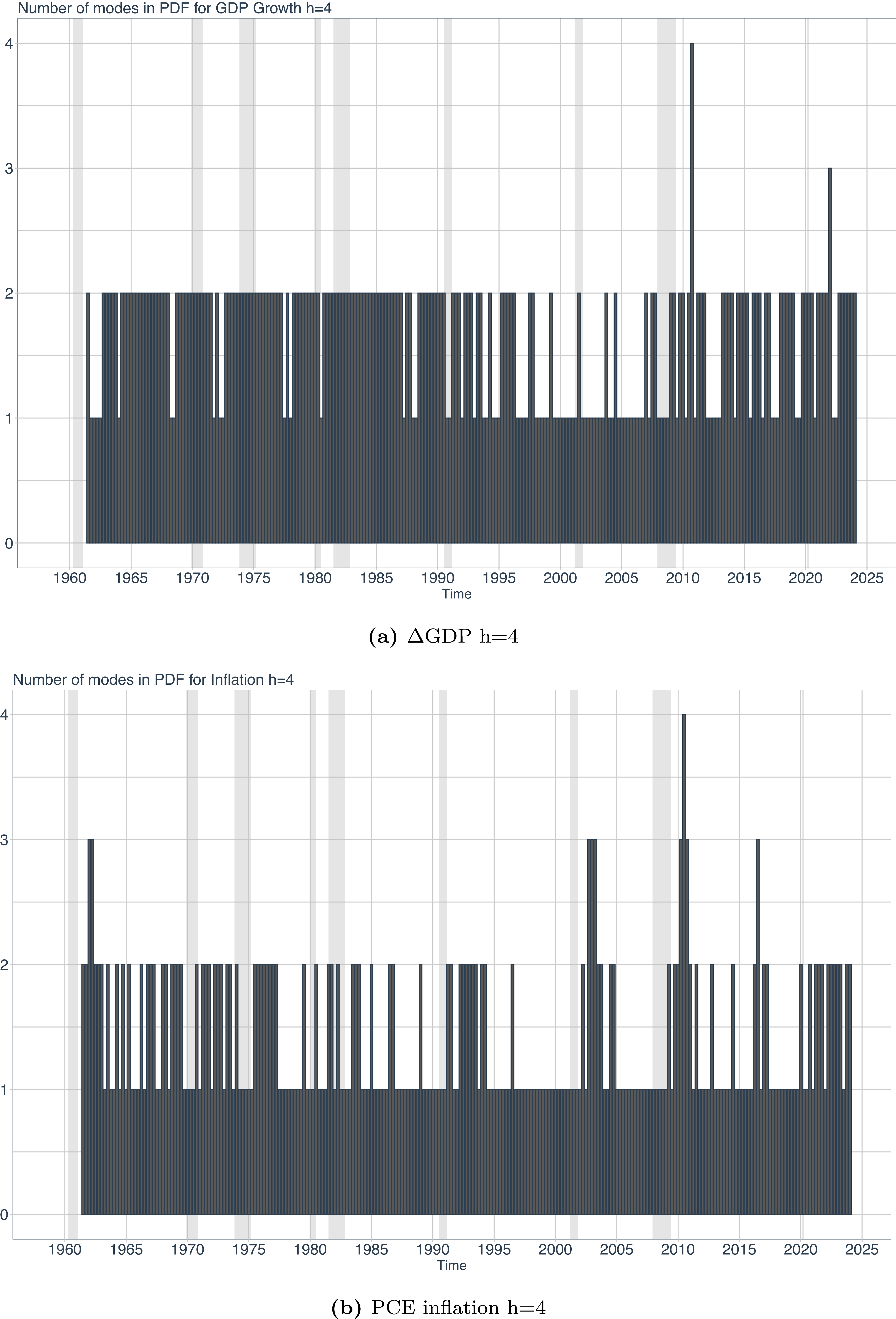
Multimodality: I use the adaptive kernel method of Portnoy and Koenker (Reference Portnoy and Koenker1989) to fit a Gaussian kernel to the implied conditional quantiles from the factor approach for both GDP growth and inflation. This approach is more flexible than the skew-t distribution of Azzalini and Capitanio (Reference Azzalini and Capitanio2003) which Adrian et al. (Reference Adrian, Boyarchenko and Giannone2019) use, as it does not force the distribution to be unimodal. In fact, using this approach, Figure 5 shows that the GDP growth distribution is bimodal most of the time and the same goes for PCE inflation, although this is more pronounced in recessionary periods. The finding echoes Adrian et al. (Reference Adrian, Boyarchenko and Giannone2021), Mitchell et al. (Reference Mitchell, Poon and Zhu2024), and Forni et al. (Reference Forni, Gambetti and Sala2025) and suggests the presence of good and bad states the economy can be expected to converge to given current economic conditions.
Count of modes in the kernel fitted distributions implied by the conditional quantiles from factor regressions for GDP growth and PCE inflation.

Conditional distributions during the financial crisis: Figure 6 shows the Gaussian kernel fitted distributions of expected GDP growth and inflation for the years of the Great Recession. The evolution of the distribution shows that even before the crisis, the GDP growth distribution had been bimodal, with a mode near zero growth and a positive mode. As the recession unfolds, the information set captured by the factors leads the expected distribution to shift leftward while maintaining the bimodality feature. This only disappears in the recovery. Contrary to this, the expected distribution of inflation is unimodal almost throughout the crisis as prices only dropped significantly toward its end. The model anticipated the deflationary episode of the third quarter of 2009 reasonably well, but over-predicts its persistence.
Four quarters ahead predicted PDFs of GDP growth and PCE inflation between Q2:2007 and Q1:2010. The year in the title of each plot is the year for which the expected distribution is computed, not the year when the expectation is formed, which would be
 $h=4$
quarters earlier.

Model evaluation: Evaluating the fit of the model is not straightforward in the case of quantile regressions, as no direct equivalent to the usual
 $R^2$
measure and its adjusted versions exists. Koenker and Machado (Reference Koenker and Machado1999) propose a metric called
 $R^1$
. This statistic evaluates the loss implied by the residuals of the quantile regression (V1) at each quantile against the alternative of running the regressions only on a constant (V0).
 \begin{align} V1_\tau &= \sum _{i=1}^T \rho _\tau \big(u_i^1\big) \end{align}
 \begin{align} V0_\tau &= \sum _{i=1}^T \rho _\tau \big(u_i^0\big) \end{align}
 \begin{align} R^1 &= 1 - \frac {V1}{V0} \end{align}
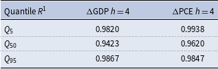
The values will be close to one if the loss of the V0 model is large relative to the V1 model. Table 4 reports the
 $R^1$
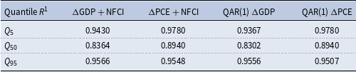
measures for the quantile regressions of GDP growth and the inflation measure at the prediction horizon of four. The performance of the model over the simple model is very good for the extreme quantiles and for the median. Especially for PCE inflation the inclusion of additional information in the predictive regressions is beneficial. In addition, Table 5 compares the fit of the model of Adrian et al. (Reference Adrian, Boyarchenko and Giannone2019) and a QAR(1) for both variables of interest using the maximum available sample including the NFCI from 1971. Both score consistently worse than the factor approach. The results suggest that the factor approach is suitably information rich.
Measures of fit from factor quantile regressions computed for the quantiles of interest

Table 4. Long description
A table comparing the performance of factor quantile regressions for GDP growth and inflation measures. The table has four rows and three columns. The columns are labeled Quantile R 1, Delta GDP h equals 4, and Delta PCE h equals 4. The rows are labeled Q 5, Q 50, and Q 95. Row 1: Q 5, 0.9820, 0.9938. Row 2: Q 50, 0.9423, 0.9620. Row 3: Q 95, 0.9867, 0.9847.
Measures of fit computed for the quantiles of interest using the specification of Adrian et al. (Reference Adrian, Boyarchenko and Giannone2019) which includes the lagged dependent variable and the NFCI or a QAR(1). Forecast horizon is
 $h=4$
, the column names are the regressors used

Table 5. Long description
A table comparing measures of fit for quantiles of interest in GDP and inflation models. The table has four rows and five columns. The columns are labeled Quantile R1, ΔGDP + NFCI, ΔPCE + NFCI, QAR(1) ΔGDP, and QAR(1) ΔPCE. The rows are labeled Q5, Q50, and Q95. Row 1: Quantile R1, 0.9430; ΔGDP + NFCI, 0.9780; ΔPCE + NFCI, 0.9367; QAR(1) ΔGDP, 0.9780. Row 2: Quantile R1, 0.8364; ΔGDP + NFCI, 0.8940; ΔPCE + NFCI, 0.8302; QAR(1) ΔGDP, 0.8940. Row 3: Quantile R1, 0.9566; ΔGDP + NFCI, 0.9548; ΔPCE + NFCI, 0.9556; QAR(1) ΔGDP, 0.9507.
4.3 Quantile impulse responses
Figure 7 shows the responses of the predicted conditional quantiles to the 100bp contractionary monetary policy shock at horizon
 $h=4$
. The IRFs can be interpreted as follows: a 100 bp monetary policy shock alters current macroeconomic conditions such that the expected year-on-year distribution of GDP growth and inflation is affected as portrayed. For example, all forecasted quantiles for GDP growth decrease on impact and return to zero after around five quarters. The initial reaction of downside risk is stronger than for upside risk. The median result is in line with the mean effect depicted in Figure 1. This suggests that the predictions for GDP growth become more pessimistic and the distribution shifts to the left. As distinct from this, we observe a clear spreading of the predicted distribution of PCE inflation, which is a result of the left tail moving further left and the right tail moving further right. Since the median also moves to the left (again in line with the mean results), this implies a skewing of the distribution as well as a spreading—the right tail becomes longer.
Point estimates of the impulse responses of the quantiles of h = 4 GDP growth and PCE inflation to a 100bp monetary policy shock. Bootstrapped 90% confidence intervals. Top graph is Q5 response, middle graph is Q50 response, bottom graph is Q95 response.

From the responses of the conditional quantiles we can compute how the contractionary monetary policy shock affects the interquantile range and the (Kelley) skewness in each case. Both the predicted GDP growth and inflation distributions get spread out. The skewness of GDP growth decreases relative to the steady state, for PCE inflation it becomes more positive, as shown in Figure 8.
Response of interquantile range (top) and non-normalized Kelley skewness (bottom) to the 100 bp contractionary monetary policy shock. All responses are at
 $h=4$
. 90% bootstrap intervals shaded in gray.

To explore the effects of monetary policy shocks on the conditional quantiles in more detail, I compute the forecast error variances as well as a historical decomposition for the fitted time series’ of each quantile for the
 $q=4$
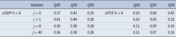
primitive shocks. This provides some information about whether the movement in the quantiles is largely attributable to monetary policy or rather to the other three unidentified shocks. The results are reported in Table 6. The monetary policy shock explains a sizable share of the variation in the conditional quantiles of GDP growth, especially of the lower tail. This suggests that policymakers should indeed take the ramifications of their decisions for growth risks into account. Furthermore, the short term importance of monetary policy for the upper tail of the predicted distribution of inflation is around 45% which decreases to 16% over the horizon of 40 periods.
I compute the contribution of the monetary policy shocks according to equation (14) together with the time series of the structural shocks
 $u_t$
. The residual is the difference between the fitted quantile and the monetary policy shock’s contribution.
The results of this exercise are shown in Figure 9. The plots reveal that the monetary policy shock played an important role in the downside risk during the 1970s recession, but has been keeping the 5th quantile higher during the Great Moderation. Its overall impact on the quantiles for inflation is limited to the early sample between the 1960s and the 1980s. If anything, it seems to have somewhat contained excessive upside risk after the year 2000. In summary, while there are some signs that monetary policy can combat downside growth risks and upside inflation risks, the results of the model suggest a historically small role as a tool for containing macroeconomic risk.
4.4 Density IRFs
The changes in the full conditional distributions are depicted in Figure 10. Differences with respect to the baseline are plotted in Figure 11 together with bootstrapped 90% confidence intervals. In response to the monetary policy shock, the predicted distribution of GDP growth shifts left and the left mode becomes more distinguished. The effect recedes after around two quarters and the distribution is nearly back to its initial shape after eight quarters. This result is not fully mirrored for an expansionary shock. In the case of inflation, the initial distribution is slightly right-skewed. In line with the description above, this skewness is further increased by the monetary policy contraction, but reversed by an expansion. Moreover, we can see the second mode being pushed further to the right for the contraction which suggests that the central bank is unable to contain upside inflation risk while reducing prices on average. The contraction rather induces additional uncertainty into the economy which makes a wider range of future inflation values likely.
Forecast error variance decomposition of GDP growth quantiles and inflation quantiles to a monetary policy shock at different forecast horizons,
 $j$
periods after the event of the shock

Table 6. Long description
A table with four rows and six columns comparing forecast error variance decomposition of GDP growth and inflation quantiles to a monetary policy shock at different horizons. The table is divided into two sections: GDP growth (ΔGDP h = 4) and inflation (ΔPCE h = 4). Each section has four rows labeled j = 0, j = 1, j = 8, and j = 40, representing different forecast horizons. The columns are labeled Q05, Q50, and Q95 for both GDP growth and inflation. Row 1: j = 0, ΔGDP h = 4, Q05, 0.37; Q50, 0.43; Q95, 0.20; ΔPCE h = 4, Q05, 0.10; Q50, 0.00; Q95, 0.45. Row 2: j = 1, ΔGDP h = 4, Q05, 0.41; Q50, 0.44; Q95, 0.30; ΔPCE h = 4, Q05, 0.10; Q50, 0.03; Q95, 0.32. Row 3: j = 8, ΔGDP h = 4, Q05, 0.36; Q50, 0.38; Q95, 0.28; ΔPCE h = 4, Q05, 0.11; Q50, 0.05; Q95, 0.16. Row 4: j = 40, ΔGDP h = 4, Q05, 0.36; Q50, 0.38; Q95, 0.28; ΔPCE h = 4, Q05, 0.11; Q50, 0.07; Q95, 0.16.
Historical decomposition of the quantiles of GDP growth and inflation into the contribution of the unit variance monetary policy shock and the residual component.

Figure 9. Long description
The figure contains multiple line graphs depicting historical decomposition of quantiles of GDP growth and inflation. Panel A shows the decomposition for GDP growth, while Panel B shows the decomposition for inflation. Each panel is divided into three sub-panels representing different quantiles: Q05, Q50, and Q95. The x-axis for all sub-panels represents quarters from 1960 to 2025. The y-axis represents the percentage contribution. The graphs include lines for MP Shock, Quantile, and Residual components, with MP Shock in red, Quantile in black, and Residual in gray. The graphs show fluctuations in the contributions of these components over time, with notable peaks and troughs. The trends indicate varying impacts of monetary policy shocks and residual components on GDP growth and inflation across different quantiles.
Response of fitted distribution to 100 bp monetary policy shocks. Steady state distribution is fitted to the predicted distribution using the median values of the regressors. All forecast distributions are at h = 4.

Figure 10. Long description
Panel A: A line graph shows the impact of a positive MP shock on the mean distribution of inflation at horizon 4. The x-axis ranges from -5 to 10, and the y-axis ranges from 0 to 0.5. The graph includes two lines representing Horizon 0 and Horizon -1, with Horizon 0 peaking around 0 on the x-axis and Horizon -1 showing a similar but slightly shifted peak. Panel B: Another line graph illustrates the impact of a positive MP shock on the mean distribution of inflation at horizon 4. The x-axis ranges from -5 to 10, and the y-axis ranges from 0 to 0.5. This graph includes lines for Horizon -1 and Horizon 2, with both lines peaking around 0 on the x-axis. Panel C: A line graph depicts the impact of a positive PCE inflation shock on the mean distribution of inflation at horizon 4. The x-axis ranges from -5 to 10, and the y-axis ranges from 0 to 0.5. The graph includes lines for Horizon -1 and Horizon 12, with both lines peaking around 0 on the x-axis. Panel D: Another line graph shows the impact of a negative MP shock on the mean distribution of inflation at horizon 4. The x-axis ranges from -5 to 10, and the y-axis ranges from 0 to 0.5. This graph includes lines for Horizon 0 and Horizon -1, with both lines peaking around 0 on the x-axis. Panel E: A line graph illustrates the impact of a negative MP shock on the mean distribution of inflation at horizon 4. The x-axis ranges from -5 to 10, and the y-axis ranges from 0 to 0.5. The graph includes lines for Horizon -1 and Horizon 2, with both lines peaking around 0 on the x-axis. Panel F: Another line graph depicts the impact of a negative PCE inflation shock on the mean distribution of inflation at horizon 4. The x-axis ranges from -5 to 10, and the y-axis ranges from 0 to 0.5. This graph includes lines for Horizon -1 and Horizon 12, with both lines peaking around 0 on the x-axis.
Response of fitted distribution to 100 bp monetary policy shocks. Steady state distribution is fitted to the predicted distribution using the median values of the regressors. All forecast distributions are at h = 4.

Figure 11. Long description
Panel A: Four line graphs depict the impact of positive monetary policy shocks on the difference in the density of inflation at different horizons. Each graph has a horizontal axis labeled with values ranging from -5 to 10 and a vertical axis labeled Density Difference ranging from -0.4 to 0.5. The graphs show varying trends with peaks and troughs, indicating the response of inflation density to positive shocks over different time horizons. Panel B: Four line graphs depict the impact of negative monetary policy shocks on the difference in the density of inflation at different horizons. Each graph has a horizontal axis labeled with values ranging from -5 to 10 and a vertical axis labeled Density Difference ranging from -0.5 to 0.5. The graphs show varying trends with peaks and troughs, indicating the response of inflation density to negative shocks over different time horizons.
5. Discussion
The results presented above taken together suggest that contractionary monetary policy may be an inadequate tool for controlling macroeconomic risk. Rather, it appears to exacerbate the “bad” equilibria existing in the conditional distributions of GDP growth and inflation. Returning inflation to lower levels is associated with significant macroeconomic and uncertainty costs. Possible explanations for these mechanisms can be traced back as far as Bernanke (Reference Bernanke1983). Given that contractionary monetary policy increases the range of possible outcomes, this may activate an “options” channel which induces agents to save instead of invest which contributes to lower growth. Explanations for non-linear amplification of monetary policy are usually drawn from financial frictions (see Brunnermeier and Sannikov (Reference Brunnermeier and Sannikov2014) or Adrian et al. (Reference Adrian, Boyarchenko and Giannone2021)). For example, if financial conditions are tightened after the monetary policy intervention, this can cause constraints on borrowing to start to bind pushing the economy away from the flexible equilibrium. The plethora of possible amplification mechanisms—spanning financial markets, labor markets and consumer confidence channels—suggests that it is necessary to allow for a rich set of conditioning variables to characterize the conditional distributions of GDP growth and inflation as I have done here.
A striking feature of the results is the continued presence of multiple modes in the distributions of GDP growth and inflation. The emergence of additional modes in the conditional distributions of GDP growth and inflation can be seen as evidence that monetary policy can lead to multiplicity of economic equilibria. Such multiplicity can arise for example if the central bank’s reaction to inflation is insufficiently strong in a New-Keynesian framework (Lubik and Schorfheide, Reference Lubik and Schorfheide2004). This leads to an indeterminate propagation of monetary policy with potentially many outcomes receiving positive probability. Lubik and Schorfheide (Reference Lubik and Schorfheide2004) show that depending on the selected equilibrium contractionary shocks can decrease growth by different magnitudes, which is in line with the two modes in the predicted GDP growth distribution representing different equilibria where the contraction has different intensities. Similarly, they show that depending on the selected equilibrium prices can in fact increase shortly after the introduction of the contractionary policy, which is observable in the right mode of Figure 10 in panel c).
Multiple equilibria are a salient feature of economic models which feature some form of coordination failure (Cooper and John, Reference Cooper and John1988). A discussion in the context of global games is provided in Morris and Shin (Reference Morris and Shin2002). Essentially, multiplicity arises if the optimal strategies of the involved players affect the others’ strategies, for example in supplier networks, demand across different economic sectors, or trade. Special cases of such failures are the famed bank runs of Diamond and Dybvig (Reference Diamond and Dybvig1983) as extended to the financial panics of Gertler et al. (Reference Gertler, Kiyotaki and Prestipino2020) or the uncertainty traps of Fajgelbaum et al. (Reference Fajgelbaum, Schaal and Taschereau-Dumouchel2017). All these models have in common a deterioration of fundamentals which keeps agents from jointly coordinating on the first-best actions which leads them to get stuck in a less desirable equilibrium. The research in the present paper shows that there exists the possibility to select among different equilibria almost throughout the entire sample period since the 1960s. While multiplicity is stronger during the first half of the sample as suggested in Lubik and Schorfheide (Reference Lubik and Schorfheide2004), strategic complementarities are present throughout.
6. Conclusion
In this paper I propose a new method to assess how monetary policy shocks influence the full conditional distributions of GDP growth and inflation in the US by combining a dynamic factor model with predictive quantile regressions. The methodology is general enough to study the response of any variable included in the data set. I show that the predictive distributions of both variables shift to the left in response to the shock and that downside growth risks are exacerbated by the shock even more than upside risks are reduced. Moreover, the short horizon predicted inflation distribution spreads out. This suggests that monetary policy may open up uncertainty channels which can have real consequences. While the policy achieves a reduction in median expected inflation, it creates potential for more extreme future inflation outcomes as well. Moreover, I show that contractionary shocks can create additional modes in the expected distributions of interest, which lead to significant increase in the probability that growth will decline by much more than on average and even carries the potential for the policy being ineffective in reducing inflation at all.
Supplementary material
The supplementary material for this article can be found at https://doi.org/10.1017/S1365100526101199.
Acknowledgements
For a very helpful discussion I thank Fabio Cesare Bagliano. I am grateful to Luca Gambetti, Tatjana Dahlhaus, Christian Brownlees, Luca Sala, and participants of the SoFie Summer School, the Simposio de la Asociación Española de Economía, the Bellaterra Macro Club, the Vilfredo Pareto PhD Workshop in Turin, and the BSE PhD Jamboree for very helpful comments and suggestions. This paper has benefited from very helpful comments from the editor and two anonymous referees. I acknowledge funding through grant FPI PRE2020-093941 and grant 2021 SGR 00194 from the Generalitat de Catalunya. The views expressed herein are those of the author and do not necessarily represent the views of the European Commission. This work was written largely when the author was employed at the Universitat Autonoma de Barcelona and Barcelona School of Economics. All remaining errors are mine.


 h=4


 ×

 h=4
 h=4


 h=4
 j



