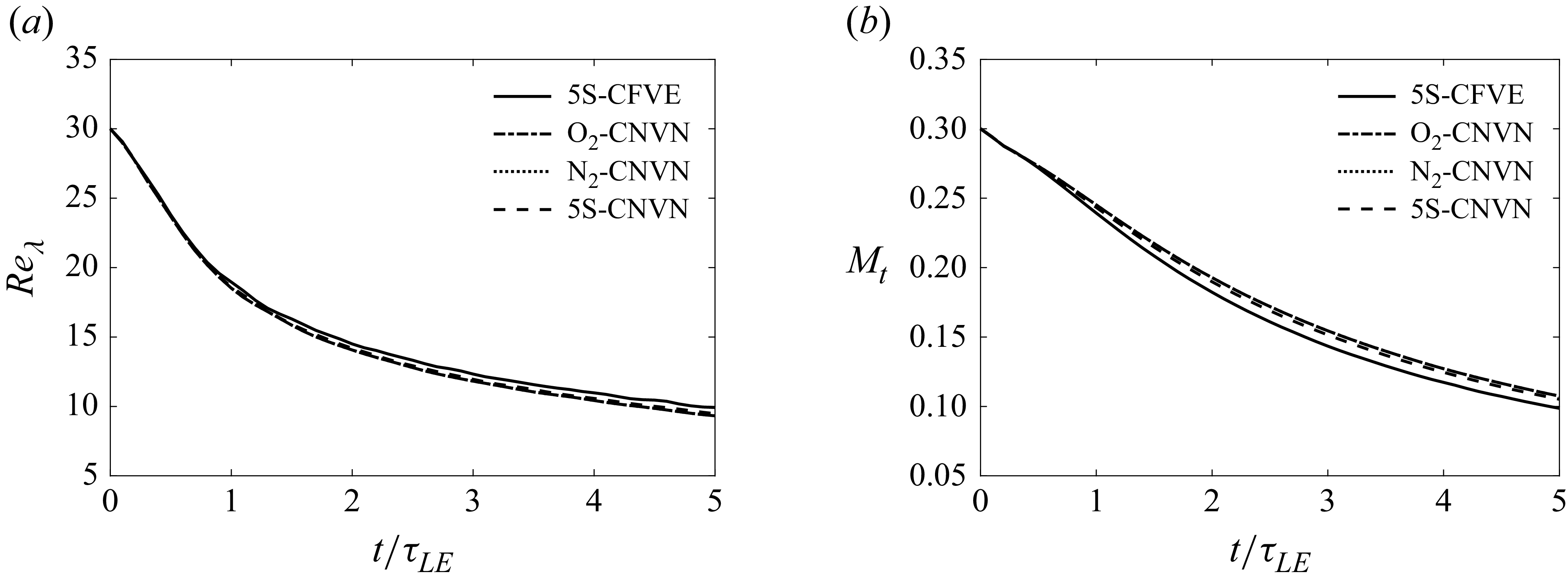
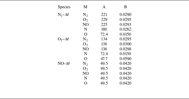
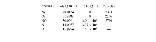
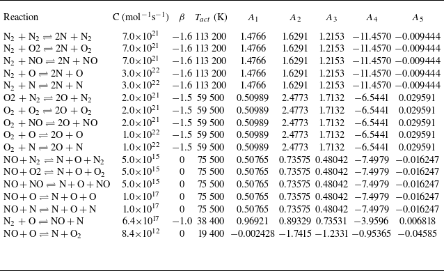
1. Introduction
High-speed flows past hypersonic vehicles are complex. Not only are these flow fields already turbulent, but the extreme velocities in such flows generate high-temperature zones, which may trigger vibrational excitation of the constituent molecules. At still higher temperatures, these excitations may become vigorous enough to dissociate multi-atomic constituent molecules of the air, triggering some chemical reactions, as well. Even though these vibrational excitations and chemical reactions do have inherent tendencies to attain equilibrium with the local temperature, the characteristic times over which such relaxation to equilibrium is attained are comparable to the inherent time scales of fluid advection and turbulence. Such a flow field is said to be in a state of thermochemical non-equilibrium (Gnoffo et al. Reference Gnoffo, Weilmuenster, Hamilton, Olynick and Venkatapathy1999; Anderson Reference Anderson2000; Colonna, Bonelli & Pascazio Reference Colonna, Bonelli and Pascazio2019). To improve our understanding of the turbulent flow past hypersonic vehicles, we must examine how the thermochemical non-equilibrium process present in a vibrationally excited and chemically reacting air mixture affects turbulence.
The overarching goal of this study is to employ direct numerical simulation (DNS) to examine the influence of thermochemical non-equilibrium of the reacting air mixtures on the velocity gradient and the pressure-Hessian tensors. The dynamics of the velocity gradient tensor is often employed to understand various turbulence processes of interest: energy cascades (Girimaji & Zhou Reference Girimaji and Zhou1995), material element deformation (Batchelor Reference Batchelor1952; Girimaji & Pope Reference Girimaji and Pope1990), scalar mixing (O’Neill & Soria Reference O’Neill and Soria2005; Meneveau Reference Meneveau2011), enstrophy production (Zheng et al. Reference Zheng, Yang, Wang and Chen2022) and intermittency (Li & Meneveau Reference Li and Meneveau2005, Reference Li and Meneveau2006). The pressure-Hessian tensor plays a significant role in the evolution of velocity gradients in a turbulent flow field as this tensor is the mathematical manifestation of the pressure field in the exact evolution equation of the velocity gradient tensor (more on this in § 2.2). In addition to offering a means to improve our understanding of turbulence, a study of the velocity gradient and the pressure-Hessian tensor also has the potential to directly help in the development of closure models for alternate methods of turbulence computations, such as the Lagrangian probability density function (p.d.f.) methods for both incompressible (Girimaji & Pope Reference Girimaji and Pope1990; Pope Reference Pope1994) and compressible turbulence (Sinha & Girimaji Reference Sinha and Girimaji2009, Reference Sinha and Girimaji2011).
DNS-based studies on the dynamics of velocity gradients and pressure-Hessian tensors have been performed earlier by several researchers both in incompressible and compressible turbulence. These simulations have been performed over a variety of canonical flow fields, such as decaying turbulence, forced isotropic turbulence, boundary layer flows and mixing layers. In incompressible turbulent flows, the pioneering DNS-based work by Ashurst et al. (Reference Ashurst, Kerstein, Kerr and Gibson1987) explored the alignment between vorticity and eigenvectors of the strain-rate tensor in isotropic turbulence. Their finding showed that there is a strong tendency for vorticity to align with the intermediate strain-rate eigenvector. This alignment was later confirmed through experimental studies by Tsinober, Kit & Dracos (Reference Tsinober, Kit and Dracos1992). These behaviours have been consistently observed in subsequent studies, contributing to an improved understanding of the dynamics of the velocity gradient tensor in incompressible flows. Several other studies have examined the statistical properties of the vorticity field, strain-rate tensor and enstrophy transfer by highlighting the significant aspects of these turbulence dynamics (Soria et al. Reference Soria, Sondergaard, Cantwell, Chong and Perry1994; Hamlington, Schumacher & Dahm Reference Hamlington, Schumacher and Dahm2008; Wallace Reference Wallace2009; Mathew & Ghosh Reference Mathew and Ghosh2011; Zhou et al. Reference Zhou, Nagata, Sakai, Ito and Hayase2016; Carter & Coletti Reference Carter and Coletti2018). Kalelkar (Reference Kalelkar2006) performed a detailed analysis of the pressure fluctuations and of the same structural aspects of the pressure-Hessian tensor. Further details on various studies of the velocity gradient and the pressure-Hessian tensor in incompressible turbulent flows can be found in the comprehensive review by Meneveau (Reference Meneveau2011).
In the field of compressible turbulence, the pioneering work of Sinha & Girimaji (Reference Sinha and Girimaji2009) derived the exact evolution equations for the velocity gradient and the pressure-Hessian tensors using the state equation of an ideal gas, along with the continuity, momentum and internal energy equations. Their research highlighted the significance of examining the exact evolution of the pressure-Hessian tensor in the context of compressible velocity gradient dynamics. Continuing along this line of research, Sinha & Girimaji (Reference Sinha and Girimaji2010) used DNS data to study the impact of compressibility on the structure of velocity gradients and flow-field topology. They examined the behaviour of turbulence statistics as a function of local dilatation and found that conditioned at various discrete dilatation levels, compressible turbulence exhibits distinctly different behaviours compared with the typical patterns seen in incompressible turbulence. Wang et al. (Reference Wang, Shi, Wang, Xiao, He and Chen2012) found that in highly compressed regions, the eigenvalue ratios and the dynamics of the strain-rate tensor can significantly deviate, highlighting the role of strong local compression in enhancing enstrophy production. Furthermore, various authors have investigated the influence of Mach number, local dilatation rate and other compressibility parameters on the dynamics of the velocity gradients (Sinha & Girimaji Reference Sinha and Girimaji2011; Danish, Suman & Srinivasan Reference Danish, Suman and Srinivasan2016; Johnson & Meneveau Reference Johnson and Meneveau2018; Zheng et al. Reference Zheng, Wang, Noack, Li, Wan and Chen2020). However, all this research focused merely on the influence of fluid compressibility on the dynamics of velocity gradient and the pressure-Hessian tensor. No influence of thermochemical non-equilibrium was simulated or examined in these studies.
The effects of chemical non-equilibrium alone on nitrogen recombination in decaying turbulence were investigated by Martın et al. (Reference Martın, Dopazo and Valiño1998). They found that exothermic reactions lead to increased temperature fluctuations. In another study, the influence of chemical reactions on compressible turbulence has been studied by Jaberi, Livescu & Madnia (Reference Jaberi, Livescu and Madnia2000), who investigated the influence of exothermic chemical reactions alone (no vibrational non-equilibrium). The study identified how exothermic reactions could alter molecular transport coefficients, thereby affecting temperature fluctuations and velocity gradient parameters within decaying compressible turbulent flows. Duan & Martín (Reference Duan and Martín2011) studied the turbulence–chemistry interactions (TCIs) within hypersonic turbulent boundary layers. They concluded that while TCI significantly affects local chemical production rates, it appears to have minimal impact on macroscopic properties such as skin friction and wall heat flux at solid surfaces. Teng et al. (Reference Teng, Wang, Li and Chen2021) investigated the impact of exothermic reactions on turbulent flow past a flat plate, focusing on how these reactions influence a turbulent flow field.
The influence of vibrational non-equilibrium alone on compressible turbulence has been examined by Neville et al. (Reference Neville, Nompelis, Subbareddy and Candler2014). Based on their study of decaying turbulence, the authors concluded that vibrational non-equilibrium reduces fluctuations in thermodynamic variables without affecting the decay rate of turbulence kinetic energy. Donzis & Maqui (Reference Donzis and Maqui2016), as well as Zheng et al. (Reference Zheng, Wang, Alam, Noack, Li and Chen2021), conducted simulations of forced isotropic turbulence under conditions of vibrational non-equilibrium, analysing how energy is distributed across various internal modes based on the vibrational relaxation time scale. Further, Zheng et al. (Reference Zheng, Yang, Wang and Chen2022) examined how vibrational non-equilibrium affects enstrophy production in compressible isotropic turbulence, using large-scale thermal forcing. Their results indicate that while solenoidal components are the main drivers of enstrophy production, dilatational effects also play a significant, though localised, role, highlighting the complex interactions within turbulent flow topologies under non-equilibrium conditions. Srivastava, Bhat & Sinha (Reference Srivastava, Bhat and Sinha2024) investigated how different Damköhler numbers affect the turbulence statistics under vibrational non-equilibrium conditions in homogeneous isotropic flows.
Candler (Reference Candler2019) simulated the combined influence of vibrational and chemical non-equilibrium flows over conical bodies, highlighting the significance of finite-rate processes, including vibrational energy relaxation, chemical reactions and surface catalysis on turbulence dynamics. Another study by Di Renzo & Urzay (Reference Di Renzo and Urzay2021) provides a detailed analysis of hypersonic boundary layers at suborbital enthalpies through direct numerical simulations. The study focuses on how vibrational excitation, chemical kinetics and aerodynamic heating influence the dynamics of transitions and the properties of turbulent flows. The research offers critical insights into the thermochemical-induced challenges in designing hypersonic vehicles due to increased thermochemical loads on the fuselage. Passiatore et al. (Reference Passiatore, Sciacovelli, Cinnella and Pascazio2022) examines how a turbulent boundary layer behaves under conditions of thermal and chemical non-equilibrium. Using DNS, their study highlights significant interactions between turbulent mixing and non-equilibrium processes, emphasising the role of molecular nitrogen in causing the vibrational non-equilibrium and proposing a vibrational Prandtl number for modelling the turbulent flux of vibrational energy. Kerkar & Ghosh (Reference Kerkar and Ghosh2024) conducted DNS of decaying turbulence, including both non-equilibrium conditions to assess their collective impact at moderate Reynolds and turbulent Mach numbers. They examine the velocity-related statistics, such as turbulent kinetic energy and dissipation. Recently, Srivastava & Sinha (Reference Srivastava and Sinha2025) have examined the effects of vibrational and chemical non-equilibrium on the dynamics of velocity gradients and pressure-Hessian tensors in compressible decaying turbulence. The authors investigated the specific roles of inertial, vibrational and chemical mechanisms through DNS of isotropic decaying turbulence. Even though these authors have examined the effects of vibrational non-equilibrium on the dynamics of velocity gradients and the pressure-Hessian tensor in the presence of chemical reactions, all their simulations are initiated with a flow field having only molecular oxygen
 $({\textrm{O}}_2)$
, and the reactions considered therein are entirely endothermic dissociation reactions.
Unlike a purely
 ${\textrm{O}}_2$
-based or purely
 ${\textrm{N}}_2$
-based chemical system, which involves only endothermic reactions, a reactive air mixture includes both endothermic and exothermic chemical reactions. This distinction is expected to significantly alter the vibrational and chemical relaxation processes (more on this in §§ 4.1–4.3). While the study conducted by Srivastava & Sinha (Reference Srivastava and Sinha2025) provides useful conceptual insights, it must be extended to consider a reacting air mixture that more accurately represents an Earth-like atmosphere. Thus, the goal of this study is to examine the influence of vibrational and chemical non-equilibrium on the evolution of the velocity gradients and the pressure-Hessian tensor in a chemically reacting air mixture. The present study focuses on identifying the influence of weak but finite compressibility at moderate turbulent Mach numbers on volume-averaged velocity-gradient and pressure–Hessian statistics. To achieve this goal, we perform the following tasks in this paper.
-
(i) We perform a set of direct numerical simulations of decaying isotropic turbulence in a reacting air mixture with five species (
 ${\textrm{N}}_2, {\textrm{O}}_2, {\textrm{NO}}, {\textrm{N}}$
and
${\textrm{O}}$
) and a set of 17 chemical reactions.
-
(ii) We examine the behaviour of the velocity gradient and pressure-Hessian statistics in these simulations and compare these statistics with those from simulations where only molecular oxygen or molecular nitrogen is present initially. Further, we also make comparisons with the behaviour in a non-reacting air-like mixture.
-
(iii) We isolate and examine the various mechanisms of the vibrational and chemical non-equilibrium processes that lead to the altered nature of velocity and pressure-Hessian tensors in the presence of a chemically reacting air mixture.


The paper is structured as follows. Section 2 provides a brief overview of the governing equations and the important aspects of exact evolution equations of the pressure-Hessian and velocity gradient tensors, which have been earlier derived by Srivastava & Sinha (Reference Srivastava and Sinha2025). Section 3 outlines the various DNS simulation cases employed in this work and describes the plan of study. Section 4 presents the results and discussion, including the analysis of vibrational relaxation, energy spectra and mechanisms governing the evolution of the velocity gradient tensor under various thermochemical non-equilibrium conditions. Furthermore, we examine the relative significance of inertial, vibrational and chemical mechanisms in shaping the behaviour of the pressure-Hessian and velocity gradient tensors. We discuss the significance and implications of this work in § 5. Finally, the paper summarises the key findings and limitations of this study in § 6.
2. Governing equations
The primary objective of this study is to improve our understanding of how vibrational and chemical non-equilibrium conditions influence the dynamics of velocity gradients and pressure-Hessian tensors in a reactive air mixture. For such a flow field, the exact evolution equations of the velocity gradient and the pressure-Hessian tensor have been derived recently by Srivastava & Sinha (Reference Srivastava and Sinha2025). Subsequent to this derivation, the authors performed DNS studies with the initial flow field having only molecular oxygen as the initial condition and considered only dissociation reactions in their flow field. Nonetheless, their derivation of the governing equations of the velocity gradient and the pressure-Hessian tensor was general and is indeed applicable to the reacting air mixtures, as well. We include a brief summary of these equations here. The reader may refer to Srivastava & Sinha (Reference Srivastava and Sinha2025) for full details.
To present an orderly summary of the governing equations of the velocity gradient and the pressure-Hessian tensor, we first present the governing equations of instantaneous density, velocity and internal energy (§ 2.1). We refer to these quantities as raw fields. Subsequently, in § 2.2, we present an overview of the evolution equations of the velocity gradient and the pressure-Hessian tensors (Srivastava & Sinha Reference Srivastava and Sinha2025). We refer to these quantities as the derivative tensors.
2.1. Governing equations of the raw variables
We begin with the conservation of mass, Newton’s second law of motion and the first law of thermodynamics. These laws lead to the governing equations of density, momentum and energy:
 \begin{align} \frac {\partial \rho }{\partial t} + \frac {\partial (\rho u_j)}{\partial x_j} & = 0, \end{align}
 \begin{align} \frac {\partial (\rho u_i)}{\partial t} + \frac {\partial (\rho u_i u_j)}{\partial x_j} &= -\frac {\partial p}{\partial x_i} + \frac {\partial \tau _{ji}}{\partial x_j}, \end{align}
 \begin{align} \frac {\partial \rho e}{\partial t} + \frac {\partial (\rho e u_j)}{\partial x_j} = -\frac {\partial (pu_j)}{\partial x_j}+\frac {\partial (u_i \tau _{\textit{ij}})}{\partial x_j} & - \frac {\partial q_j^{\textit{tr}}}{\partial x_j} - \frac {\partial q_j^{{V}}}{\partial x_j} - \frac {\partial }{\partial x_j} \left ( \sum _{s=1}^{ns} \rho _s u_{sj}^D h_s \right ), \end{align}
 \begin{align} \frac {\partial \rho _s}{\partial t} + \frac {\partial (\rho _s u_j)}{\partial x_j} &= -\frac {\partial \big(\rho _s u_{sj}^D\big)}{\partial x_j} + \dot {\omega }_s, \end{align}
 \begin{align} \frac {\partial (\rho _m e_{V_m})}{\partial t} + \frac {\partial (\rho _m e_{V_m} u_j)}{\partial x_j} = -\frac {\partial q_{j_m}^{{V}}}{\partial x_j} - \frac {\partial }{\partial x_j} & \left ( \rho _m u_{\textit{mj}}^D e_{V_m} \right ) + \sum _{m=1}^{nd} (Q_{{T-V}_m} + \dot {\omega }_m e_{V_m}). \end{align}
In (2.1),
 $\rho$
denotes the density of the mixture,
 $u_j$
represents the instantaneous velocity vector in the
 $j$
th direction, and
 $t$
and
 $x_j$
are time and spatial coordinates, respectively, in the Cartesian coordinate system. In the momentum equation (2.2),
 $p$
denotes the pressure derived from the ideal gas law as applied to a mixture of gases. Using Dalton’s law of partial pressures, we express the thermal equation of state as
 \begin{equation} p = T \sum _{s=1}^{ns} \rho _s R_s, \end{equation}
where
 $T$
is the temperature of the gas in Kelvin,
 $R_s$
is the gas constant for species
 $s$
in
 ${\textrm{J kg}}^{-1}\,{\textrm{K}}^{-1}$
and
 $\rho _s$
is the density of species
 $s$
.
The viscous stress tensor,
 $\tau _{ji}$
, is modelled according to the equation:
 \begin{equation} \tau _{ji} = 2 \mu \left [\frac {1}{2} \left (\frac {\partial u_i}{\partial x_j} + \frac {\partial u_j}{\partial x_i}\right ) - \frac {1}{3}\delta _{ji} \frac {\partial u_k}{\partial x_k}\right ], \end{equation}
where
 $\mu$
is the dynamic viscosity of mixture and
 $\delta _{ji}$
is the Kronecker delta. In practical flows at hypersonic speed, variation in temperature leads to variation in viscosity also. However, in this work, our motivation is to merely isolate the direct influence of thermochemical non-equilibrium on the velocity gradient and the pressure-Hessian physics. Thus, the viscosity (
 $\mu$
) is held constant in our simulations. At the initial instant, the viscosity for each gas is computed using the Blottner correlation (Blottner, Johnson & Ellis Reference Blottner, Johnson and Ellis1971), and this constant value is then maintained during the entire simulation period. This approach is consistent with our earlier studies (Srivastava et al. Reference Srivastava, Bhat and Sinha2024; Srivastava & Sinha Reference Srivastava and Sinha2025). The Blottner equation for the species-specific viscosity coefficients is given by
 \begin{equation} \mu _s = 0.1 \times \exp \left [ \left ( A_{B,s} \ln (T) + B_{B,s} \right ) \ln (T) + C_{B,s} \right ], \end{equation}
where
 $A_{B,s}$
,
 $B_{B,s}$
and
 $C_{B,s}$
are empirical coefficients for species
 $s$
, and
 $T$
is the translational–rotational temperature. These coefficients are summarised in Appendix A.1.
Equation (2.3) governs the total energy per unit mass (
 $e$
), of the flow, which is a summation of different energy components within the gas mixture. The total energy is expressed as
 \begin{equation} e = \underbrace {\sum _{s=1}^{ns} Y_s C_{v,s} T}_{\text{translational-rotational energy}} + \underbrace {\frac {1}{2} u_i u_i}_{\text{kinetic energy}} + \underbrace {\sum _{m=1}^{nd} Y_m e_{V_m}}_{\text{vibrational energy}} + \underbrace {\sum _{s=1}^{ns} Y_s h_s^0}_{\text{chemical energy}}. \end{equation}
The translational–rotational energy is calculated as the product of the mass fraction (
 $Y_s = {\rho _s}/{\rho }$
) of each species
 $s$
, specific heat at constant volume
 $C_{v,s}$
and the local temperature
 $T$
. Contribution
 $ {1}/{2} (u_i u_i)$
represents the kinetic energy per unit mass of the mixture. Vibrational energy accounts for the energy stored in the vibrational modes of diatomic species, indexed by
 $m$
. Chemical energy is calculated as the sum of the standard enthalpy of formation,
 $h_s^0$
, of each species
 $s$
, weighted by its mass fraction. Here,
 $ns$
represents the total number of species and
 $nd$
is the number of diatomic species within the mixture.
The species continuity (2.4) describes the evolution of
 $\rho _s$
. The quantity
 $\rho _su_{sj}^D$
, represents the diffusive flux of species
 $s$
in the
 $j$
th direction. The production rate of species
 $s$
due to chemical reactions is denoted by
 $\dot {\omega }_s$
. The mixture density
 $\rho$
, required for calculating the mass fractions, is the sum of the partial densities of all species, expressed as
 $\rho = \sum _{s=1}^{ns} \rho _s$
. The specific heat at constant volume for any species
 $s$
, denoted as
 $C_{v,s}$
, includes contributions from both translational and rotational modes, which can be expressed as
 \begin{equation} C_{v,s} = C_{v,s}^{({tr})} + C_{v,s}^{({rot})}. \end{equation}
For translational modes, the specific heat is
 \begin{equation} C_{v,s}^{({tr})} = \frac {3}{2} R_s, \end{equation}
while for rotational modes, it depends on the molecular structure:
 \begin{equation} C_{v,s}^{({rot})} = \begin{cases} R_s & \text{for diatomic species}, \\ 0 & \text{for monoatomic species}. \end{cases} \end{equation}
The enthalpy per unit mass of a species
 $s$
, denoted by
 $h_s$
, is formulated as
 \begin{equation} h_s = C_{v,s} T + \frac {p_s}{\rho _s} + e_{Vs} + h_s^0, \end{equation}
where
 $p_s$
is the partial pressure for individual species. Thermal and vibrational heat fluxes, represented by
 $q_j^{\textit{tr}}$
and
 $q_j^{{V}}$
, respectively, in the
 $j{\textrm{th}}$
direction, follow Fourier’s law of heat conduction and are measured in
 ${\textrm{J s}}^{-1}\,{\textrm{m}}^{-2}$
. The diffusion fluxes, denoted by
 $\rho _s u_{sj}^D$
, are modelled by a modified version of Fick’s law (Sutton & Gnoffo Reference Sutton and Gnoffo1998). This is expressed as
 \begin{equation} \rho _s u_{sj}^D = -\rho D_s \frac {\partial Y_s}{\partial x_j} + \rho _s \sum _{s=1}^{ns} D_s \frac {\partial Y_s}{\partial x_j}. \end{equation}
In (2.14), the first term on the right-hand side represents the effective diffusion velocity, while the second term accounts for a mass correction factor. This correction is essential for maintaining mass conservation in the continuity equation, particularly when dealing with species that have varying diffusion coefficients. The model for diffusion velocity employed in this work neglects the contribution from molecular weight gradients. However, this formulation allows for a variable, species-specific mass diffusion coefficient that accounts for local variations in temperature and species properties. This approximation is consistent with several other numerical studies (see, for example, Casseau et al. Reference Casseau, Palharini, Scanlon and Brown2016; Passiatore et al. Reference Passiatore, Sciacovelli, Cinnella and Pascazio2022) and is justified in detail by Sutton & Gnoffo (Reference Sutton and Gnoffo1998). For further discussion on the validity and impact of this simplification, the reader is referred to the thorough analysis provided by Sutton & Gnoffo (Reference Sutton and Gnoffo1998). The effective diffusion coefficient,
 $D_s$
, of species
 $s$
in the gaseous mixture is computed as
 \begin{equation} D_s = \frac {k_s^{({tr})} {Le}}{\rho C_{p,s}^{({tr})}}, \end{equation}
where
 $k_s^{({tr})}$
is the translational–rotational thermal conductivity in
 ${\textrm{Js}}^{-1}\,{\textrm{m}}^{-1}\,{\textrm{K}}^{-1}$
and
 $C_{p,s}^{({tr})}$
is the specific heat at constant pressure for species
 $s$
.
The translational–rotational thermal conductivity (
 $k_s^{({tr})}$
) for each species is computed using expressions based on kinetic theory, consistent with the models for multi-component, high-temperature gas mixtures (Vincenti & Kruger Reference Vincenti and Kruger1982; Park Reference Park1989). In our study, the Lewis number,
 $Le$
, is set to unity following the common practice for air-like mixtures in high-speed flows (Martın et al. Reference Martın, Dopazo and Valiño1998; Park Reference Park1993). For the main species in air,
 ${\textrm{N}}_2$
and
 ${\textrm{O}}_2$
, the Lewis number remains close to unity, typically within the range
 $0.8$
–
 $1.2$
across the temperature range relevant to our simulations (Gupta et al. Reference Gupta, Yos, Thompson and Lee1990). This approximation implies equal rates of thermal and mass diffusion, simplifying the coupling between energy and species transport in the present context.
Equation (2.5) governs the evolution of the vibrational energy for each diatomic species
 $m$
at every grid point and time step. This means that a separate vibrational energy equation is solved for each diatomic species (e.g. N
 $_2$
, O
 $_2$
and NO) present in the flow. The vibrational energy per unit mass
 $e_{V_m}$
of each species
 $m$
evolves according to this equation, providing direct access to the vibrational energy fields for each diatomic species. The vibrational temperature
 $T_{V_m}$
for each diatomic species is subsequently computed a posteriori, if required, using the harmonic oscillator relation given by (2.16). For diatomic species, the corresponding vibrational temperature,
 $T_{V_m}$
, specific to each diatomic species is defined by the equation:
 \begin{equation} e_{V_m} = \begin{cases} \frac {\theta _m R_m}{\exp (\theta _m / T_{V_m}) - 1} & \text{if the species is diatomic}, \\ 0 & \text{if the species is monoatomic}. \end{cases} \end{equation}
In (2.16),
 $\theta _m$
is the characteristic vibrational temperature, indicating the energy level at which the molecular vibrations significantly influence the thermodynamic behaviour of the species. The vibrational source term gets contributions from two mechanisms. The first mechanism is the energy exchange between vibrational and translational modes, quantified as
 $\sum _{m=1}^{nd} Q_{T-V_m}$
, and the second mechanism shows the net vibrational energy change due to molecular production or depletion, represented by
 $\sum _{m=1}^{nd} \dot {\omega }_m e_{V_m}$
. The vibrational–translational energy exchange is calculated using the Landau–Teller model (Landau Reference Landau1936):
 \begin{equation} \sum _{m=1}^{nd} Q_{T-V_m} = \sum _{m=1}^{nd} \rho _m \frac {e_{V_m}^* - e_{V_m}}{\tau _{\textit{Vm}}}, \end{equation}
where
 $e_{V_m}^*$
is the vibrational energy per unit mass in equilibrium with the local temperature (
 $T$
), and is defined as
 \begin{equation} e_{V_m}^* = \frac {\theta _m R_m}{\exp (\theta _m / T) - 1}. \end{equation}
The symbol
 $\tau _{\textit{Vm}}$
in (2.17) represents the molar-averaged Landau–Teller relaxation time, which characterises the time required for the vibrational energy (
 $e_V$
) of a diatomic species to relax towards its equilibrium state
 $e_V^*$
. As modelled by the Landau–Teller equation (2.17), this relaxation process is influenced by collisions within the gas mixture. These collisions can occur between diatomic molecules (
 ${\textrm{N}}_2$
,
 ${\textrm{O}}_2$
and
 ${\textrm{NO}}$
), and between diatomic and monoatomic molecules (
 ${\textrm{N}}$
and
 ${\textrm{O}}$
). Consequently,
 $\tau _{\textit{Vm}}$
is defined using the molar concentrations of these species as a weighted average:
 \begin{equation} \tau _{\textit{Vm}} = \sum \limits _{s=1}^{ns} \frac {\rho _s}{M_s}\left (\sum \limits _{s=1}^{ns} \frac {{\rho _s}/{M_s}}{\tau _{m-s}}\right )^{-1}. \end{equation}
The symbol
 $\tau _{m-s}$
in (2.19) denotes the individual relaxation times for collisions between the
 $m{\text{th}}$
species and other species
 $s$
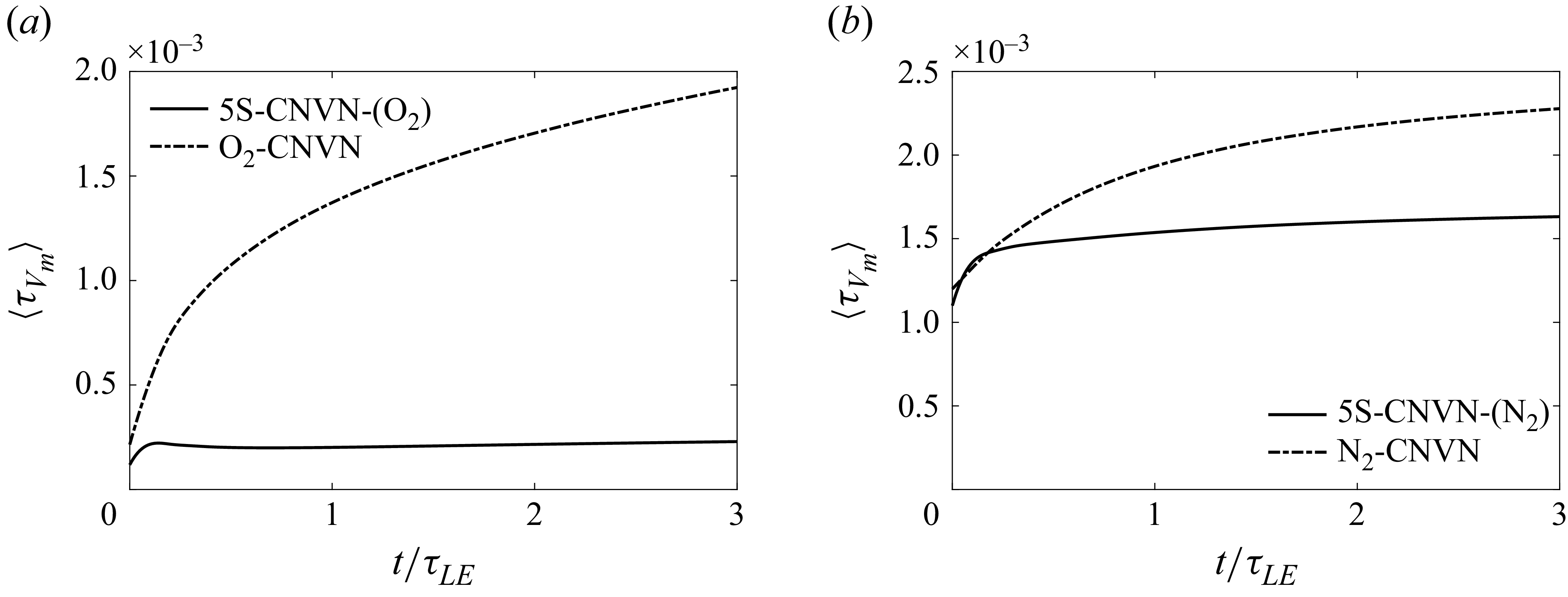
within the mixture. This approach accounts for all significant collision pairs, both diatomic–diatomic and diatomic–monoatomic, ensuring the contribution of each species in the computation of vibrational relaxation time. Equation (2.19) shows that the
 $\tau _{\textit{Vm}}$
of a given diatomic molecule (for example, the
 ${\textrm{O}}_2$
molecule) strongly depends on the composition of the mixture. Millikan and White (MW) developed a semi-empirical method to compute the relaxation times
 $\tau _{\textit{m-s}}^{\textit{MW}}$
for each species pair, applicable across a temperature range from 300 K to 8000 K (Park Reference Park1989). Recognising limitations in this formulation at temperatures above 5000 K, Park introduced a high-temperature correction, denoted
 $\tau _{\textit{m-s}}^{P}$
, to enhance the accuracy of these estimates (Park Reference Park1993):
 \begin{equation} \tau _{\textit{m-s}} = \tau _{\textit{m-s}}^{\textit{MW}} + \tau _{\textit{m-s}}^{P}. \end{equation}
The relaxation time
 $\tau _{\textit{m-s}}^{\textit{MW}}$
for interactions between a diatomic molecule
 $m$
and species
 $s$
is described by the following semi-empirical formula developed by Millikan and White:
 \begin{equation} \tau _{\textit{m-s}}^{\textit{MW}} = \frac {1}{p} \exp \big [ A_{m, s} \big (T^{-1/3} - B_{m, s}\big ) - 18.42 \big ], \end{equation}
where
 $p$
represents the pressure in atmospheres (1 atm = 101 325 Pa). The coefficients
 $A_{m,s}$
and
 $B_{m,s}$
are derived from the equations:
 \begin{equation} A_{m, s} = 1.16 \times 10^{-3} \sqrt {M_{m,s}} \theta _{m}^{4/3}\quad \text{and}\quad B_{m, s} = 0.015 M_{m,s}^{1/4}, \end{equation}
where
 $M_{m,s}$
is the reduced molecular weight, calculated as
 $M_{m,s} = {M_{m} M_s}/{M_{m} + M_s}$
, and
 $M_{m}$
and
 $M_s$
are the molecular weights of the diatomic species
 $m$
and species
 $s$
, respectively. These derived coefficients are included in Appendix A.2. Moreover, a correction factor for high temperatures, denoted
 $\tau _{\textit{m-s}}^{P}$
, is added to the Millikan and White formulation to enhance its accuracy:
 \begin{equation} \tau _{\textit{m-s}}^{P} = \frac {1}{\bar {c}_{m} \sigma _{v,m} n_{m,s}}, \end{equation}
where
 $\bar {c}_{m}$
represents the average molecular speed,
 $\sigma _{v,m}$
is the collision cross-section and
 $n_{m,s}$
is the number density of the colliding pairs. These parameters are estimated as follows:
 \begin{equation} \bar {c}_{m} = \sqrt {\frac {8 R_{m} T}{\pi }}\quad \text{and}\quad \sigma _{v,m} = 3.0 \times 10^{-21} \left (\frac {50\,000}{T}\right )^2. \end{equation}
In this work, we use 5 species and a 17-reaction model to capture the physics of reacting air mixture. These 5 species are
 ${\textrm{N}}_2$
,
 ${\textrm{O}}_2$
,
 ${\textrm{NO}}$
,
 ${\textrm{N}}$
and
 ${\textrm{O}}$
. The production or depletion of these species is described using the following set of five reversible chemical reactions (Vincenti & Kruger Reference Vincenti and Kruger1982; Park Reference Park1989):
 \begin{equation} \left . \begin{aligned} {\text{R1: }} &\quad {\textrm{N}}_2 + M \;\rightleftharpoons \; 2N + M \\ {\text{R2: }} &\quad {\textrm{O}}_2 + M \;\rightleftharpoons \; 2O + M \\ {\text{R3: }} &\quad {\textrm{NO}} + M \;\rightleftharpoons \; N + O + M \\ {\text{R4: }} &\quad {\textrm{N}}_2 + O \;\rightleftharpoons \; NO + N \\ {\text{R5: }} &\quad {\textrm{NO}} + O \;\rightleftharpoons \; N + O_2. \end{aligned} \right \} \end{equation}
In these reactions,
 $M$
represents a third body that can be
 ${\textrm{N}}_2$
,
 ${\textrm{O}}_2$
,
 ${\textrm{NO}}$
,
 ${\textrm{N}}$
or
 ${\textrm{O}}$
. The first three reactions (R1, R2 and R3) are primarily governing the dissociation and recombination processes. However, reactions R4 and R5 manage the interconversion between
 ${\textrm{NO}}$
and the elements
 ${\textrm{N}}$
or
 ${\textrm{O}}$
, called shuffle reactions. Specifically, the forward direction of reaction R4, together with the reverse direction of reaction R5, represents the Zel’dovich mechanism for nitric-oxide production (Williams Reference Williams1986). The reaction rates
 $(RR)$
corresponding to each reaction
 $(R)$
involved in (2.25) are
 \begin{equation} \left \{ \begin{aligned} {{\textit{RR}}_1} &= \sum _{m} \left [ -k_{f1,m} \frac {\rho _{{\textrm{N}}_2}} {M_{{\textrm{N}}_2}} \frac {\rho _m}{M_m} + k_{b1,m} \left (\frac {\rho _{\textrm{N}}}{M_{\textrm{N}}}\right )^2 \frac {\rho _m}{M_m} \right ] \\ {{\textit{RR}}_2} &= \sum _{m} \left [ -k_{f2,m} \frac {\rho _{{\textrm{O}}_2}} {M_{{\textrm{O}}_2}} \frac {\rho _m}{M_m} + k_{b2,m} \left (\frac {\rho _{\textrm{O}}}{M_{\textrm{O}}}\right )^2 \frac {\rho _m}{M_m} \right ] \\ {{\textit{RR}}_3} &= \sum _{m} \left [ -k_{f3,m} \frac {\rho _{{\textrm{NO}}}} {M_{{\textrm{NO}}}} \frac {\rho _m}{M_m} + k_{b3,m} \left (\frac {\rho _{\textrm{N}} \rho _{\textrm{O}}}{M_{\textrm{N}} M_{\textrm{O}}}\right ) \frac {\rho _m}{M_m} \right ] \\ {{\textit{RR}}_4} &= -k_{f4} \frac {\rho _{{\textrm{N}}_2}} {M_{{\textrm{N}}_2}} \frac {\rho _{\textrm{O}}}{M_{\textrm{O}}} + k_{b4} \frac {\rho _{{\textrm{NO}}}} {M_{{\textrm{NO}}}} \frac {\rho _{\textrm{N}}}{M_{\textrm{N}}} \\ {{\textit{RR}}_5} &= -k_{f5} \frac {\rho _{{\textrm{NO}}}} {M_{{\textrm{NO}}}} \frac {\rho _{\textrm{O}}}{M_{\textrm{O}}} + k_{b5} \frac {\rho _{{\textrm{O}}_2}} {M_{{\textrm{O}}_2}} \frac {\rho _{\textrm{N}}}{M_{\textrm{N}}}. \end{aligned} \right . \end{equation}
Finally, the net source term for each chemical species,
 $s$
, contributing to the reaction rates
 $({\textit{RR}}_1{-}{\textit{RR}}_5)$
in (2.26) due to chemical reactions is given by
 \begin{equation} \left \{ \begin{aligned} \dot {\omega }_{{\textrm{N}}_2} &= M_{{\textrm{N}}_2} ({\textit{RR}}_1+{\textit{RR}}_4) \\ \dot {\omega }_{{\textrm{O}}_2} &= M_{{\textrm{O}}_2} ({\textit{RR}}_2-{\textit{RR}}_5) \\ \dot {\omega }_{ {\textrm{NO}}} &= M_{ {\textrm{NO}}} ({\textit{RR}}_3-{\textit{RR}}_4+{\textit{RR}}_5) \\ \dot {\omega }_{\textrm{N}} &= M_{\textrm{N}} (-2{\textit{RR}}_1-{\textit{RR}}_3-{\textit{RR}}_4-{\textit{RR}}_5) \\ \dot {\omega }_{\textrm{O}} &= M_{\textrm{O}} (-2{\textit{RR}}_2-{\textit{RR}}_3+{\textit{RR}}_4+{\textit{RR}}_5). \end{aligned} \right . \end{equation}
The objective of this study is to investigate the influence of thermochemical non-equilibrium on a reacting air mixture. Thus, all our numerical simulations begin with an air-like mixture composed of mass fractions of
 $76.67\,\%\ {\textrm{N}}_{2}$
,
 $21.34\,\%\ {\textrm{O}}_{2}$
,
 $1\,\%\ {\textrm{NO}}$
,
 $0.5\,\%\ {\textrm{N}}$
and
 $0.5\,\%\ {\textrm{O}}$
. These initial values are chosen to approximate a physically realistic atmospheric air composition under hypersonic conditions, where nitrogen and oxygen are dominant, and minor species (
 ${\textrm{NO}}$
,
 ${\textrm{N}}$
and
 ${\textrm{O}}$
) are present in trace amounts (required for initialisation in hy2FOAM solver). This composition is nearly identical to that used in a previous work by Passiatore et al. (Reference Passiatore, Sciacovelli, Cinnella and Pascazio2022). The thermochemical properties of these species are provided in Appendix A.3. For the reaction kinetics, the forward reaction rate constant
 ${k}_{f}$
(see (2.26)) is modelled using a modified Arrhenius equation:
 \begin{equation} k_{f}(T_c,f) = C\,T_{c,f}^{\beta } \exp \left (-\frac {T_{act}}{T_{c,f}}\right ), \end{equation}
where
 $T_{act}$
represents the activation temperature derived from the activation energy,
 $C$
is the pre-exponential factor and
 $\beta$
is the temperature exponent. Here,
 $T_{c,f}$
is the controlling temperature of the forward reaction. The relationship defining the backwards reaction rate constant,
 ${k}_{b}$
, is expressed as follows:
 \begin{equation} {k}_{b}(T_{c,b}) = \frac {k_f(T_{c,b})}{K_{eq}(T_{c,b})}, \end{equation}
where
 $T_{c,b}$
is the controlling temperature affecting the backward reaction. Here,
 $K_{eq}$
represents the equilibrium constant for the given reaction, which varies with temperature based on empirical data (Park Reference Park1993). The empirical model for
 $K_{eq}$
, adapted from experimental results, is given by
 \begin{equation} K_{eq}(T_{c,b}) = \exp \left ( \frac {A_1 T_{c,b}}{10^4} + A_2 + A_3 \ln \left (\frac {10^4}{T_{c,b}}\right ) + A_4 \frac {10^4}{T_{c,b}} + A_5 \left (\frac {10^4}{T_{c,b}}\right )^2 \right ). \end{equation}
Here, the coefficients
 $A_1$
–
 $A_5$
depend on the local mixture number density provided in Appendix A.4. The vibration–dissociation coupling is modelled through an effective temperature,
 $T_{\textit{eff}_{m}}$
, which blends the translational–rotational temperature,
 $T$
, and the vibrational temperature of each diatomic species,
 $T_{V_m}$
, as follows (Candler Reference Candler1989):
 \begin{equation} T_{\textit{eff}_{m}} = T^{\alpha } T_{V_m}^{1-\alpha }. \end{equation}
Typically, the exponent
 $\alpha$
is set to 0.7 (Candler & Nompelis Reference Candler and Nompelis2009). Other controlling temperatures corresponding to the dissociation and exchange reactions are provided in table 1. Using (2.26)–(2.31), the source terms
 $\dot {\omega }_s$
appear in the species continuity equation (2.4) can be computed.
Temperature conditions for forward and backward reactions.

2.2. Governing equations of velocity gradient and the pressure-Hessian tensors
The primary quantities of investigation in this work are the velocity gradient tensor (
A
) and the pressure-Hessian tensor (
P
). The governing equation for the velocity gradient tensor (
 $\boldsymbol{A}$
) is obtained by taking the derivative of the instantaneous momentum equation:
 \begin{equation} \frac {{\textrm D} A_{\textit{ij}}}{{\textrm D}t} = -A_{ik} A_{\textit{kj}} - P_{\textit{ij}} + \varGamma _{\textit{ij}}. \end{equation}
The symbols
 $A_{\textit{ij}}$
and
 $P_{\textit{ij}}$
represent the
 $(ij){\textrm{th}}$
components of the velocity gradient and the pressure-Hessian tensors, respectively,
 \begin{equation} A_{\textit{ij}} = \frac {\partial u_i}{\partial x_j}\quad \text{and}\quad P_{\textit{ij}} = \frac {\partial }{\partial x_j}\left (\frac {1}{\rho }\frac {\partial p}{\partial x_i}\right ), \end{equation}
where
 $u_i$
is the
 $i{\textrm{th}}$
component of velocity and
 $x_i$
is the
 $i{\textrm{th}}$
spatial coordinate in the Eulerian description of flow. In (2.32), the material derivative is denoted by
 $ {\textrm D}/{{\textrm D}t} = {\partial }/{\partial t} + u_k ({\partial }/{\partial x_k})$
. This operator measures the temporal and advective changes of
 $A_{\textit{ij}}$
as observed with the motion of a small fluid element. The self-stretching term,
 $-A_{ik}A_{\textit{kj}}$
, captures the inertial effects on the local state of the velocity gradient tensor (Vieillefosse Reference Vieillefosse1982). The second term, the pressure-Hessian tensor
 $(\boldsymbol{P})$
, accounts for the effects of pressure and density gradients on the evolution of velocity gradients in a compressible medium. This term represents the fluid–thermodynamic coupling in compressible flows. The third term
 $\varGamma _{\textit{ij}}$
on the right-hand side of (2.32) includes higher-order gradients of the velocity gradient tensor along with density gradients. This term accounts for the influence of viscosity on the dynamics of the velocity gradient tensor. It is expressed as
 \begin{equation} \varGamma _{\textit{ij}} = \frac {\partial }{\partial x_j} \left \{ \frac {1}{\rho } \frac {\partial }{\partial x_k} \left [ \mu \left ( A_{ik} + A_{\textit{ki}} - \frac {2}{3} A_{pp} \delta _{\textit{ki}} \right ) \right ] \right \}. \end{equation}
In incompressible flows, the pressure is determined by Poisson’s equation. In contrast, in compressible flows, pressure is a direct thermodynamic variable, evolving in accordance with changes in the density and temperature fields. This difference necessitates a separate evolution equation for the pressure-Hessian tensor in compressible turbulence. Sinha & Girimaji (Reference Sinha and Girimaji2011) presented the exact evolution equation for the pressure-Hessian tensor in compressible flows, however, they did not account for vibrational non-equilibrium effects. Building on this work, Srivastava et al. (Reference Srivastava, Bhat and Sinha2024) modified the pressure-Hessian equation for vibrational non-equilibrium flows. Their study focuses on single species that are free from chemical reactions. Subsequently, Srivastava & Sinha (Reference Srivastava and Sinha2025) have derived the exact evolution equation of the pressure-Hessian tensor, including both vibrational and chemical non-equilibrium. Even though they performed all their numerical simulations starting with only pure
 ${\textrm{O}}_2$
molecules, their derivation of (2.35) is indeed generally applicable to any initial composition of the fluid mixture. The full derivation of this equation is included in Srivastava & Sinha (Reference Srivastava and Sinha2025). In this paper, we avoid the repetition of the entire derivation process and include the final form of this equation for further analysis and discussion in the context of reacting air mixtures:
 \begin{align} \frac {{\textrm D} P_{\textit{ij}}}{{\textrm D}t} &= \underbrace {\left (-A_{\textit{kj}}P_{ik}-A_{\textit{ki}}P_{\textit{kj}}-\frac {2}{5}A_{\textit{kk}}P_{\textit{ij}}\right )}_{(I)} \underbrace {-\frac {7}{5}\frac {p}{\rho }\left (\frac {\partial ^2A_{\textit{kk}}}{\partial x_i\partial x_j}-\frac {1}{\rho }\frac {\partial A_{\textit{kk}}}{\partial x_i}\frac {\ \partial \rho }{\partial x_j}\right )}_{({\textit{II}})}\nonumber \\ & \underbrace {-\left (\frac {2}{5}\frac {1}{\rho } \frac {\partial A_{\textit{kk}}}{\partial x_j}\ \frac {\partial p}{\partial x_i} + \frac {7}{5}\frac {1}{\rho } \frac {\partial A_{\textit{kk}}}{\partial x_i}\ \frac {\partial p}{\partial x_j} + \frac {1}{\rho } \frac {\partial A_{\textit{ki}}}{\partial x_j}\ \frac {\partial p}{\partial x_k} \right )}_{({\textit{III}})}\nonumber \\ & \underbrace {-\frac {2}{5} \frac {\partial }{\partial x_j} \left [ \frac {1}{\rho } \frac {\partial }{\partial x_i} \left ( \sum _{m=1}^{nd} \left ( \frac {\rho _m e_{V_m}^*}{\tau _{\textit{Vm}}} - \frac {\rho _m e_{V_m}}{\tau _{\textit{Vm}}} \right ) \right ) \right ]}_{({\textit{IV}})}\nonumber \\ & \underbrace {-\frac {2}{5} \frac {\partial }{\partial x_j} \left [ \frac {1}{\rho } \frac {\partial }{\partial x_i} \left ( \sum _{m=1}^{nd} \dot {\omega }_m e_{V_m} + \sum _{s=1}^{ns} h_s^0 \dot {\omega }_s \right ) \right ]}_{(V)}\nonumber \\ & \underbrace {+\frac {2}{5} \frac {\partial }{\partial x_j} \left [ \frac {1}{\rho } \frac {\partial }{\partial x_i} \left ( \frac {\partial }{\partial x_k} \left ( \sum _{m=1}^{nd} \rho _m u_{\textit{mk}}^D e_{V_m} - \sum _{s=1}^{ns} \rho _s u_{sk}^D h_s \right ) + \sum _{s=1}^{ns} h_s^0 \frac {\partial }{\partial x_k} \big(\rho _s u_{sk}^D\big) \right ) \right ]}_{({\textit{VI}})}. \end{align}
To improve both the mathematical clarity and physical understanding of (2.35), Srivastava & Sinha (Reference Srivastava and Sinha2025) organised different terms into categories labelled
 $(I{-}{\textit{VI}})$
. These categories represent distinct mechanisms that influence the evolution of the pressure-Hessian tensor as one follows the motion of a local fluid element under thermochemical non-equilibrium conditions. Mechanism
 $I$
in (2.35) shows the interaction between the velocity gradient tensor
 $(A_{\textit{ij}})$
and the pressure-Hessian tensor
 $(P_{\textit{ij}})$
. This interaction signifies the local stretching of the pressure-Hessian field by the velocity gradient field (Sinha & Girimaji Reference Sinha and Girimaji2011). Mechanism
 ${\textit{II}}$
involves the higher-order gradients of the velocity gradient tensor
A
interacting with the thermodynamic variable
 ${p}/{\rho }$
. According to Sinha & Girimaji (Reference Sinha and Girimaji2011), the direct inclusion of the variable
 ${p}/{\rho }$
, instead of its gradients, links this mechanism to an acoustic time scale, closely related to the local Mach number of the flow. This approach has been successfully integrated into their enhanced homogenised Euler equation
 $({\textit{EHEE}})$
model, which captures the effects of the Mach number on the dynamics of compressible flows in the velocity gradient tensor. The third mechanism introduces higher-order gradients of both the velocity gradient components and the pressure field. In their studies, the authors concentrate on compressible flows that are free from vibrational and chemical non-equilibrium effects, focusing exclusively on the changes in kinetic and translational–rotational energies within their total energy equation.
Under equilibrium conditions, the pressure-Hessian tensor development is driven solely by mechanisms
 $I$
,
 ${\textit{II}}$
and
 ${\textit{III}}$
called inertial mechanisms (refer to (2.35)). However, in the cases involving vibrational and chemical non-equilibrium physics, additional mechanisms designated as
 ${\textit{IV}}$
,
 $V$
and
 ${\textit{VI}}$
become influential. These mechanisms introduce higher-order gradients of density, temperature, vibrational temperature and chemical source terms into the evolution equation.
Mechanism
 ${\textit{IV}}$
is identified as the vibrational mechanism. This reflects the multi-species extension of the vibrational dynamics previously characterised by Srivastava et al. (Reference Srivastava, Bhat and Sinha2024). It primarily involves the gradients of both the instantaneous vibrational energy
 $(e_V)$
and its equilibrium counterpart
 $(e_V^*)$
within the flow. Mechanism
 $V$
in (2.35) addresses the effects of species production or depletion, which occur due to different chemical reactions, while mechanism
 ${\textit{VI}}$
describe the influence of species diffusion in the flow field. The latter two mechanisms
 $(V\,\text{and}\,{\textit{VI}})$
, collectively referred to as chemical mechanisms, highlight the significant role of chemical processes on the evolution of the pressure-Hessian tensor. Collectively, we refer to terms
 ${\textit{IV}}$
,
 $V$
and
 ${\textit{VI}}$
as the thermochemical non-equilibrium mechanisms. The current study focuses on investigating and understanding the behaviour of these thermochemical non-equilibrium mechanisms and their consequences on the evolution of the velocity gradient tensor (2.32) in a compressible flow field.
3. Description of DNS cases and plan of study
To achieve the objectives of this study, we have conducted a series of new direct numerical simulations. These simulations numerically solve the governing equations of the flow field, which are detailed in § 2 ((2.1)–(2.5)). The details of the numerical solver, simulation parameters, characteristic time scales, and grid and time step independence studies are presented in §§ 3.1–3.4.
3.1. Solver, numerical methods and simulation set-up
We use the hy2Foam solver, which is developed on the OpenFoam platform. The hy2Foam is designed to simulate hypersonic vehicle entries into planetary atmospheres. These scenarios involve significant kinetic energy conversion, vibrational excitation and chemical reactions among various species. The solver, extensively documented in the works of Casseau et al. (Reference Casseau, Palharini, Scanlon and Brown2016), Casseau (Reference Casseau2017), builds on the numerical methodologies of the standard OpenFOAM application rhoCentralFoam. hy2Foam is an implicit, finite-volume solver that operates in parallel across three dimensions while also supporting two-dimensional (2-D) and axisymmetric simulations. Additionally, it accommodates a wide variety of computational grids. This versatility makes it a robust tool for studying complex flows in high-temperature environments. The hy2Foam solver incorporates features that handle both vibrational and chemical non-equilibrium processes. It has been thoroughly validated for laminar flow simulations by its developer (Casseau Reference Casseau2017). Further validation of this code in simulating decaying turbulence has been performed by Srivastava et al. (Reference Srivastava, Bhat and Sinha2024) and Srivastava & Sinha (Reference Srivastava and Sinha2025).
In our studies, the computational framework solves the instantaneous continuity equations for mass (2.1), momentum (2.2), total energy conservation (2.3), species continuity (2.4) and vibrational energy evolution (2.5). Pressure calculations are performed using Dalton’s law of partial pressure for an ideal gas (2.6). The vibrational relaxation times for different species are estimated using the method developed by Millikan-White and Park (Reference Park1989, Reference Park1993).
In this study, we adopt the Kurganov, Noelle and Petrova (KNP) central-upwind scheme, a feature of the hy2Foam solver known for its second-order accuracy in processing advection terms (Kurganov, Noelle & Petrova Reference Kurganov, Noelle and Petrova2001; Greenshields et al. Reference Greenshields, Weller, Gasparini and Reese2010). We calculate diffusive fluxes using the central difference. Temporal resolution is managed through a second-order backward implicit method, which guarantees both stability and adequate precision over time. Uniform time-stepping is used in all the simulations.
3.2. Definition of non-equilibrium states and characteristic time scales
In our study, we introduce three types of time scales relevant to high-temperature compressible turbulent flows: the large-eddy turnover time (
 $\tau _{\textit{LE}}$
), which is uniquely defined for the flow field; the vibrational time scale (
 $\tau _{\textit{Vm}}$
), defined specifically for diatomic molecules
 $(m)$
; and the chemical time scale (
 $\tau _{\textit{Cs}}$
), defined individually for each species
 $(s)$
. Our analysis involves five species in total, consisting of three diatomic species (
 ${\textrm{N}}_{2}$
,
 ${\textrm{O}}_{2}$
and
 ${\textrm{NO}}$
) and two monatomic species (
 ${\textrm{N}}$
and
 ${\textrm{O}}$
). Consequently, there are three vibrational time scales corresponding to the diatomic species and five chemical time scales – one for each species. These scales are essential for understanding the interaction between turbulence, vibrational dynamics and chemical reactions.
The large eddy turnover time
 $(\tau _{\textit{LE}})$
is computed using the Taylor micro-scale (
 $\lambda$
) and the root mean squared velocity fluctuations (
 $u^{\prime}$
) (Honein & Moin Reference Honein and Moin2004):
 \begin{equation} \lambda = \sqrt {\frac {u'^2}{\langle (\partial u_1/\partial x_1)^2\rangle }}\quad \text{and}\quad u' = \sqrt {\left \langle \frac {u_1^2 + u_2^2 + u_3^2}{3} \right \rangle }, \end{equation}
which leads to the definition of
 $\tau _{\textit{LE}}$
as
 \begin{equation} \tau _{\textit{LE}} = \frac {\lambda }{u'}. \end{equation}
Following the definition of
 $\tau _{\textit{LE}}$
, the chemical time scale
 $(\tau _{\textit{Cs}})$
is calculated based on the average density and the rate of change of the chemical source term:
 \begin{equation} \tau _{\textit{Cs}} = \frac {\langle \rho \rangle }{|\langle \dot \omega _s \rangle |}, \end{equation}
where
 $\langle \rho \rangle$
represents the average density and
 $|\langle \dot \omega _s \rangle |$
denotes the magnitude of the rate of change of the chemical source term of each species, as computed in (2.27). The vibrational time scale
 $(\tau _{\textit{Vm}})$
has been previously defined in (2.19) and quantifies the time required for vibrational energy to equilibrate with translational–rotational energy, as detailed in § 2.1.
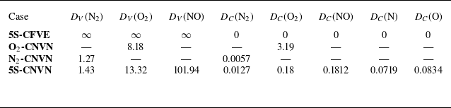
The vibrational Damköhler (
 $D_{V_m}$
) and the chemical Damköhler (
 $D_{C_s}$
) numbers for each species are defined as (Kerkar & Ghosh Reference Kerkar and Ghosh2024)
 \begin{equation} D_{V_m} = \frac {\tau _{\textit{LE}}}{\tau _{\textit{Vm}}}\quad \text{and}\quad D_{C_s} = \frac {\tau _{\textit{LE}}}{\tau _{\textit{Cs}}}, \end{equation}
where
 $\tau _{\textit{LE}}$
is the large-eddy turnover time,
 $\tau _{\textit{Vm}}$
is the vibrational relaxation time for species
 $m$
and
 $\tau _{\textit{Cs}}$
is the chemical time scale of each species. Table 2 reports the initial Damköhler numbers for each relevant species and for all simulation cases considered in this study.
Initial Damköhler numbers for vibrational and chemical relaxation in all simulation cases.

Additionally, the parameter
 $\xi _m$
measures the initial disparity between the translational–rotational and vibrational energy modes for the mth species, offering insight into the degree of non-equilibrium at the onset of our simulations. It is defined as
 \begin{equation} \xi _m = \frac {\langle T_{V_m} \rangle }{\langle T \rangle }, \end{equation}
where
 $\langle T_{V_m} \rangle$
is the volume-averaged vibrational temperature of each diatomic species and
 $\langle T \rangle$
refers to the volume-averaged translational–rotational temperature. The initial value of
 $\xi _m$
is constant for each diatomic species in every simulation (Srivastava et al. Reference Srivastava, Bhat and Sinha2024; Srivastava & Sinha Reference Srivastava and Sinha2025).
In the evaluation of high-temperature fluid dynamics, it is crucial to determine whether the flow is near a state of chemical and vibrational non-equilibrium or not. In this context, two key flow states are defined: frozen and equilibrium flows. A frozen flow is defined as one in which the reaction rate constants
 $k_f = {k}_{b} = 0$
and the vibrational relaxation time
 $\tau _{V} \approx \infty$
, signifying that there are no changes in chemical composition or internal energy modes. In contrast, an equilibrium flow is characterised by infinitely high reaction rates
 ${k}_{f} = {k}_{b} \approx \infty$
and a vibrational relaxation time
 $\tau _{V} = 0$
, which permits immediate adaptation of internal energy modes to changing conditions. However, it should be noted that in practical scenarios, neither type of flow occurs exactly as described (Anderson Reference Anderson2000). Whether a flow can be assumed to be in local equilibrium or must be considered frozen depends on the relative magnitudes of the characteristic time scales of the flow. Local equilibrium can be assumed, if
 $\tau _{\textit{LE}} \gg \tau _{\textit{Char}}$
, while a flow is considered frozen if
 $\tau _{\textit{LE}} \ll \tau _{\textit{Char}}$
, where
 $\tau _{\textit{Char}}$
is the characteristic time scale for the vibrational energy or chemical reactions to approach equilibrium. If these conditions are not distinctly met, the flow is typically in a state of non-equilibrium. This paper investigates the influence of such non-equilibrium flows on the evolution of the velocity gradient and the pressure-Hessian tensors.
3.3. Simulation parameters and cases
Numerical simulations of decaying turbulence are conducted within a cubic computational domain. Each side of the cube measures
 $2\pi$
. The grid is uniformly structured and configured with resolutions ranging from
 $192^3$
to
 $512^3$
grid points, to demonstrate grid independence. Periodic boundary conditions are implemented on opposite faces of the cube. The initial velocity field conditions are chosen to be solenoidal (divergence-free) and have zero mean velocity. The following equation defines the initial turbulence energy spectrum:
 \begin{equation} E(\kappa , t=0) = A_0 \kappa ^4 \exp \left (-2\frac {\kappa ^2}{\kappa _0^2}\right ), \end{equation}
where
 $A_0$
is the amplitude of the spectrum,
 $\kappa$
represents the wave number magnitude and
 $\kappa _0$
is the wave number at which the energy spectrum function peaks (
 $\kappa _0=4$
). Equation (3.6) is the identical spectrum function as employed by Honein & Moin (Reference Honein and Moin2004), Chen et al. (Reference Chen, Wen, Wang and Guo2020), Srivastava et al. (Reference Srivastava, Bhat and Sinha2024), Srivastava & Sinha (Reference Srivastava and Sinha2025).
The initial conditions of simulation are characterised by several non-dimensional parameters: the Taylor microscale-based Reynolds number
 $(Re_{\lambda })$
, turbulent Mach number
 $(M_t)$
, Prandtl number
 $({\textit{Pr}})$
and the initial ratio of the mean vibrational temperature to the mean temperature
 $(\xi _m)$
.
The definitions for
 ${\textit{Re}}_{\lambda }$
and
 $M_t$
are as follows:
 \begin{equation} Re_{\lambda } = \sqrt {\frac {20}{3 \nu \epsilon }} K\quad \text{and}\quad M_t = \sqrt {\frac {2K}{n R \langle T \rangle }}, \end{equation}
where
 $\nu$
is the kinematic viscosity,
 $\epsilon$
is the rate of energy dissipation,
 $K$
represents the turbulence kinetic energy and
 $\langle T \rangle$
denotes the average temperature. Here,
 $\langle \boldsymbol{\cdot }\rangle$
indicates the volume-averaged or mean value of the quantity of interest and
 $n$
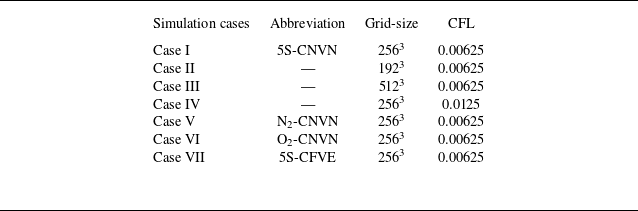
is the ratio of the specific heat capacities at constant pressure to that at constant volume. Various simulations which are employed in this study are listed in table 3. The grid size, Courant–Friedrichs–Lewy (CFL) conditions and abbreviated identifiers for various simulation cases are mentioned in this table. In all simulations, the initial turbulent Mach number (
 $M_t$
) and the Reynolds number based on the Taylor microscale (
 ${\textit{Re}}_{\lambda }$
) are
 $0.3$
and
 $30$
, respectively. The availability of our computational resources restricts the chosen values of the Reynolds and the Mach numbers. Nonetheless, we have ensured that up to these values of the Reynolds and the Mach numbers, our results are grid-independent and time-step-independent in terms of all higher-order statistics of interest used in this study (more on this in § 3.4). Further, the initial ratio of vibrational to local temperature (
 $\xi _m$
) is chosen to be
 $0.5$
for all cases and for all diatomic species. The Prandtl number
 $({\textit{Pr}})$
is
 $0.72$
.
DNS cases employed in this study.

Case I simulation (table 3) begins with a mixture of molecular nitrogen
 $({\textrm{N}}_2)$
and molecular oxygen
 $({\textrm{O}}_2)$
, nitrogen oxide
 $( {\textrm{NO}})$
, atomic nitrogen
 $({\textrm{N}})$
and oxygen
 $({\textrm{O}})$
. This simulation employs a chemical reaction model consisting of 5 species and 17 reactions, as detailed in (2.25). Additionally, the vibrational relaxation process is modelled using the Landau–Teller model. We call this simulation as the 5-species, chemical non-equilibrium, vibrational non-equilibrium (5S-CNVN) case.
Case II and Case III simulations have identical settings as Case I, except for the differences in grid size. Case II has
 $192^3$
cells and Case III has
 $512^3$
cells, respectively. Case IV is identical to Case I except that the time step employed in Case IV is twice that employed in Case I.
Case V maintains all parameters from Case I, but begins with pure molecular nitrogen, including only one chemical reaction – the dissociation of molecular nitrogen. Throughout the later stages of this simulation, only
 ${\textrm{N}}_{2}$
or
 ${\textrm{N}}$
are present. This case is referred to as the nitrogen-chemical non-equilibrium, vibrational non-equilibrium (
 ${\textrm{N}}_{2}$
-CNVN) case.
Similarly, Case VI begins with pure molecular oxygen and involves only the dissociation reaction of molecular oxygen. This case is designated as the oxygen-chemical non-equilibrium, vibrational non-equilibrium (
 ${\textrm{O}}_{2}$
-CNVN) case.
Case VII is a simulation which starts with an air-like mixture of various species (same as Case I), but no chemical reactions are allowed; that is, a chemically frozen mixture. Further, the vibrational excitation process is assumed to be in equilibrium with the local temperature at all times. We call this case as the 5-species, chemical frozen vibrational equilibrium (5S-CFVE) case.
Case I simulation (5S-CNVN) is our primary simulation case wherein we will identify the influence of vibrational and chemical non-equilibrium on the evolution of the velocity gradient and the pressure-Hessian tensors in a reacting-air mixture. Case I simulation results are compared with Case II and Case III simulation results to demonstrate that a
 $256^3$
grid employed in Case I is adequate to resolve all scales of motion with
 ${\textit{Re}}_{\lambda }=30$
and
 $M_t=0.3$
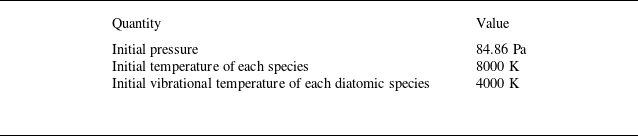
. Case I results are compared with the Case IV results to demonstrate that the employed time step is adequate to resolve all scales of motion in the Case I simulation. These demonstrations are presented in § 3.4. All dimensional simulation parameters corresponding to the 5S-CNVN case are summarised in table 4. In all simulation cases, the fluctuating temperature and fluctuating density are set to be zero initially (Sarkar et al. Reference Sarkar, Erlebacher, Hussaini and Kreiss1991; Ristorcelli & Blaisdell Reference Ristorcelli and Blaisdell1997; Samtaney, Pullin & Kosović Reference Samtaney, Pullin and Kosović2001; Srivastava et al. Reference Srivastava, Bhat and Sinha2024; Srivastava & Sinha Reference Srivastava and Sinha2025).
Initial dimensional parameters for the 5S-CNVN case.

The behaviour of the pressure-Hessian tensor and the velocity gradient tensor in the presence of thermochemical non-equilibrium has earlier been investigated by Srivastava & Sinha (Reference Srivastava and Sinha2025). However, in their simulation, only endothermic chemical reactions involving oxygen atoms and molecules are considered. In contrast, in a chemically reacting air mixture, wherein both nitrogen and oxygen diatomic molecules are present, the vibrational and chemical non-equilibrium processes may be modified further. An Earth-like planetary atmosphere is a mixture of more than one type of diatomic molecule. Further, the chemical composition of this mixture may change continuously as the flow field evolves. The presence of multiple types of diatomic molecules leads not only to the possibility of endothermic dissociation reactions, but also to several exothermic recombination reactions involving the nascent nitrogen and oxygen atoms available in the mixture. With multiple reacting species (collision partners) in the mixture, the vibrational relaxation processes of the individual nitrogen and oxygen molecules may be significantly altered compared with simulations that include only one type of diatomic molecule (in accordance with (2.19)). Thus, in line with the identified objectives of this work, we wish to contrast how different the influence of thermochemical non-equilibrium processes is in a chemically reacting air mixture when compared with (i) a simulation in which only oxygen is present and (ii) a simulation where only nitrogen is present. In § 3.4, we present extensive comparisons of Case I (5S-CNVN) results with Case V (
 ${\textrm{N}}_2$
-CNVN) and Case VI (
 ${\textrm{O}}_2$
-CNVN) results. Further, comparisons are also made with the results of simulation Case VII, which represents the baseline behaviour of the pressure-Hessian and velocity gradient tensor in the complete absence of chemical and vibrational non-equilibrium. In simulation Case VII, Terms IV and V in the evolution equation of the pressure-Hessian tensor remain identically zero at all times due to the chemically frozen and vibrationally equilibrated assumptions. Term VI, which is related to species diffusion, also remains zero in our simulations because the initial composition is specified as spatially uniform across the domain. However, we acknowledge that Term VI could be non-zero if fluctuations in the initial species mass fractions were introduced.
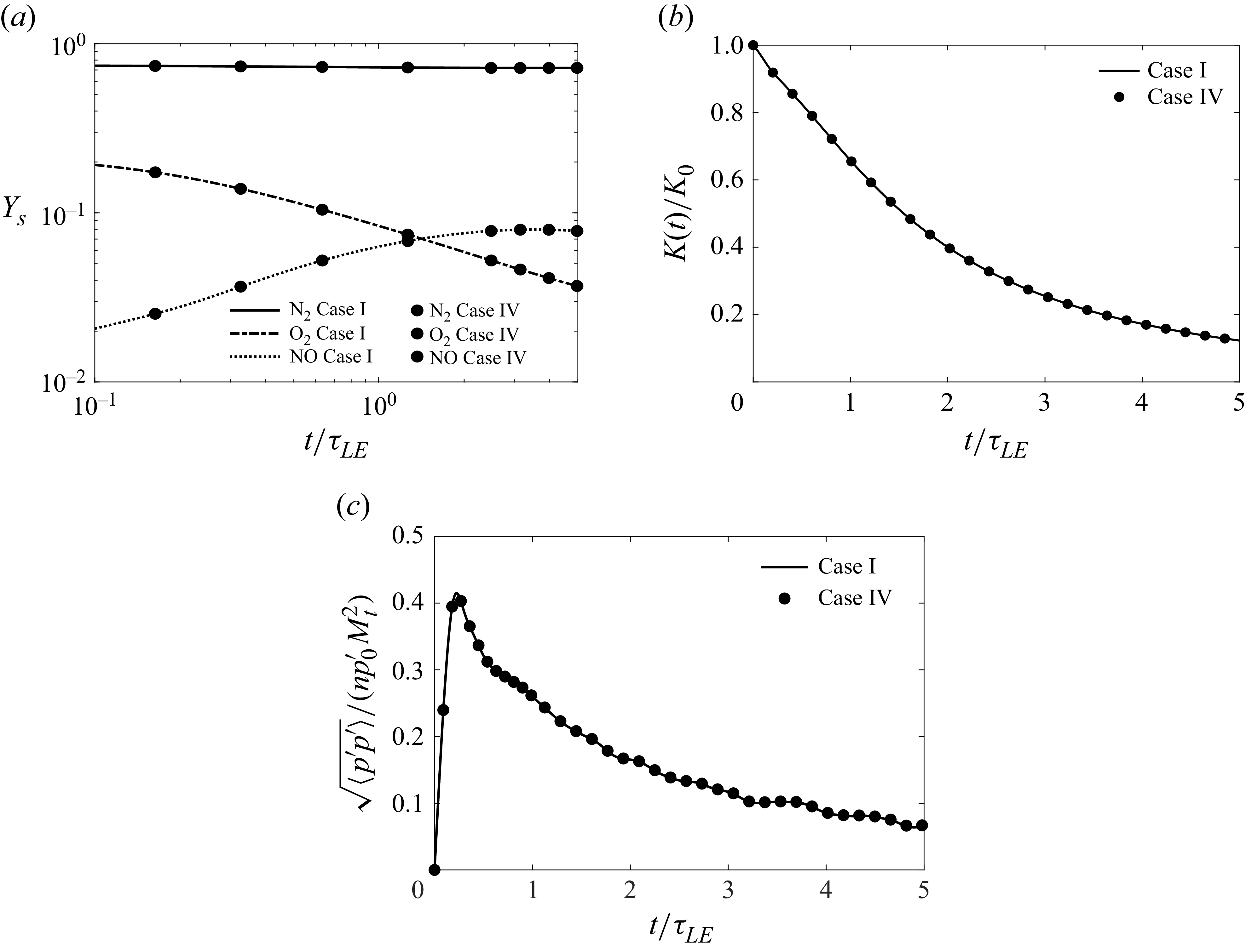
Grid independence: temporal evolution of (a) species mass fractions, (b) turbulence kinetic energy and (c) r.m.s. of pressure in simulation Cases I, II and III.

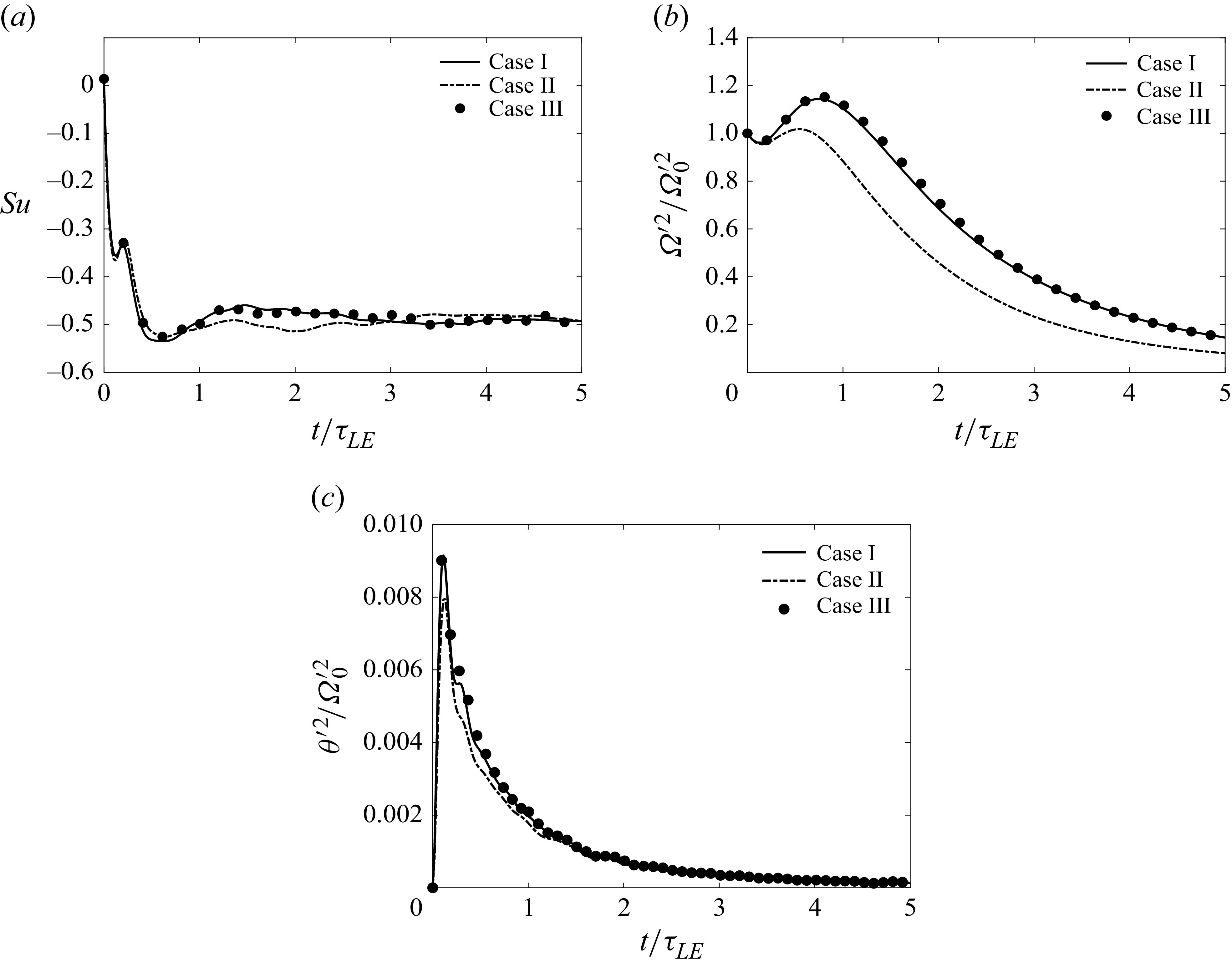
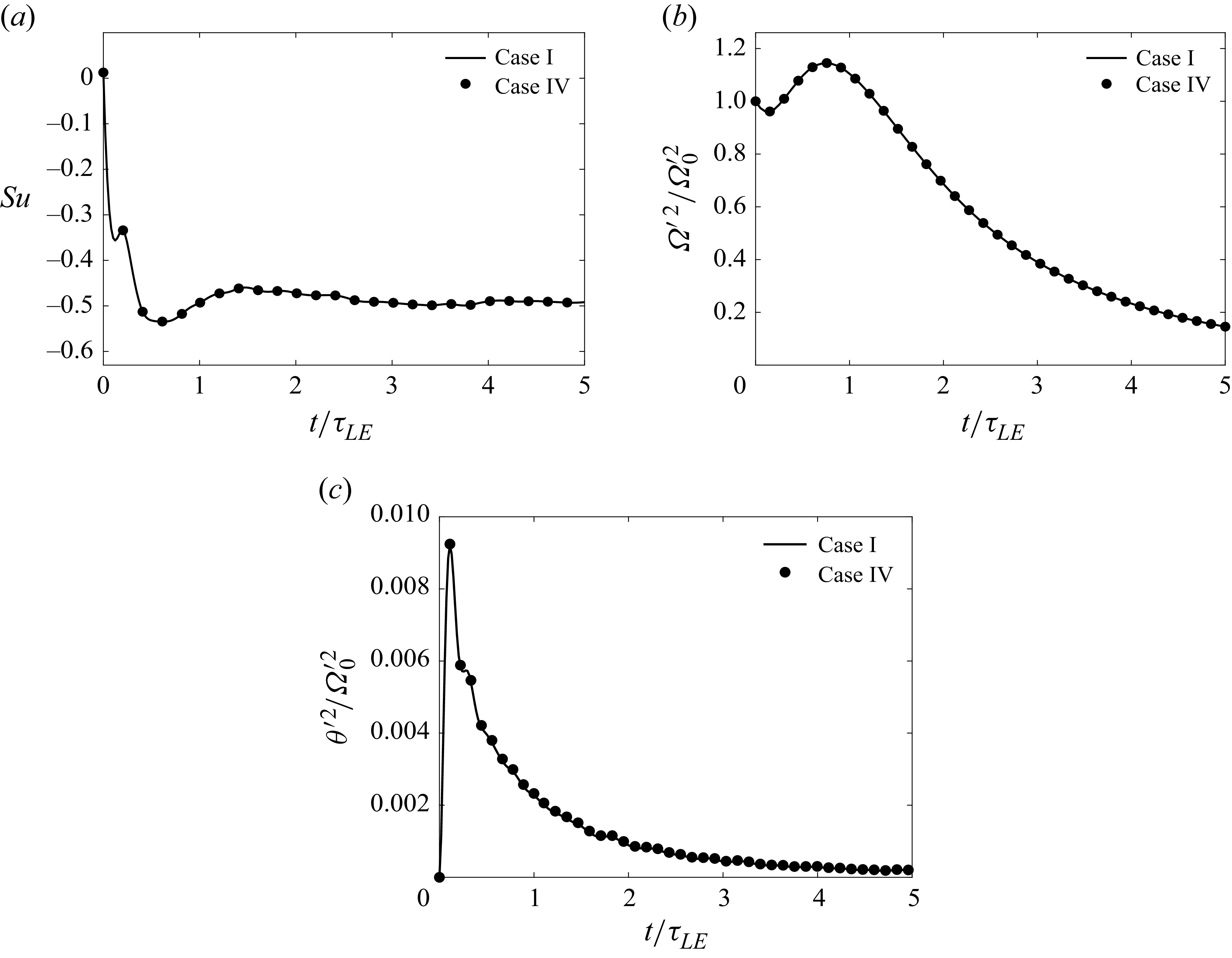
Grid independence: temporal evolution of (a) skewness, (b) vorticity fluctuations and (c) dilatational fluctuations in simulation Cases I, II and III.

3.4. Grid independence and time step independence studies
We have performed extensive grid and time step independence studies employing results from simulation Cases I–IV. We present figures 1 and 2 to demonstrate grid independence and figures 3 and 4 to demonstrate time step independence. The temporal evolution of species mass fractions
 $(Y_s)$
, turbulent kinetic energy
 $(K)$
and root mean square (r.m.s.) pressure fluctuations
 $(p^{\prime})$
is shown in figure 1(a–c), respectively. The data for figure 1(b) are normalised by their initial values, whereas the data for figure 1(c) are normalised by
 $np^{\prime }_oM_{to}^2$
, where
 $o$
denotes the initial value of the quantity. Moreover, other statistical characteristics, such as skewness
 $(S_u)$
, vorticity fluctuations
 $(\varOmega ')$
and dilatational fluctuations
 $(\theta ')$
, are examined across various grid resolutions and are shown in figure 2(a–c), respectively. The quantity
 $\varOmega '$
is defined as
 \begin{equation} \varOmega ' = {\left \langle \varOmega _i \varOmega _i \right \rangle }^{1/2}, \end{equation}
where
 $\varOmega _i$
is the
 $i{\textrm{th}}$
component of the instantaneous vorticity vector. The quantity
 $\theta '$
is defined as
 \begin{equation} \theta ' = {\left \langle \left (\frac {\partial u_i}{\partial x_i} \right )^2\right \rangle }^{1/2}. \end{equation}
While
 $\varOmega '$
is a measure of the strength of the vortical fluctuations,
 $\theta '$
is a measure of the dilatational fluctuations. The evolution of skewness (
 $S_u$
) of the velocity gradient is described as
 \begin{equation} S_u=\frac {\left \langle \left [ \left ( \frac {\partial u_1}{\partial x_1} \right )^3 + \left ( \frac {\partial u_2}{\partial {x}_2} \right )^3 + \left ( \frac {\partial u_3}{\partial {x}_3} \right )^3 \right ] / 3 \right \rangle }{\left \langle \left [ \left ( \frac {\partial u_1}{\partial {x}_1} \right )^2 + \left ( \frac {\partial u_2}{\partial {x}_2} \right )^2 + \left ( \frac {\partial u_3}{\partial {x}_3} \right )^2 \right ] / 3 \right \rangle ^{3/2}}. \end{equation}
Minimal differences between the
 $256^3$
and
 $512^3$
grid resolutions can be observed in figures 1 and 2. Over five eddy turnover times (defined in (3.2)), the maximum percentage error observed in skewness between these two resolutions does not exceed
 $2.5\,\%$
. These findings confirm that the results on the
 $256^3$
grid are sufficiently independent from further refinement of the grid. Consequently, this grid size is used for all other simulations (Cases IV–VII) employed in this study. Figures 3 and 4 show negligible differences (less than 1 %) between the simulations for Case I and Case IV in terms of time step independence.
Time step independence: temporal evolution of (a) species mass fractions, (b) turbulence kinetic energy, (c) r.m.s. of pressure in simulation Cases I and IV.

Time step independence: temporal evolution of (a) skewness, (b) vorticity fluctuations and (c) dilatational fluctuations in simulation Cases I and IV.

4. Results and discussion
In § (4.1), we first analyse the evolution of mean and fluctuating temperatures across various simulation cases to understand the vibrational relaxation processes between translational–rotational and vibrational modes under non-equilibrium conditions. The thermal relaxation process of the chemically reacting air mixture (5S-CNVN) simulation case is compared with the
 ${\textrm{N}}_2$
-CNVN and
 ${\textrm{O}}_2$
-CNVN simulation cases. Section 4.2 presents the analysis of compressibility, turbulence intensity and the energy cascade. In § 4.3, we evaluate the vibrational and chemical non-equilibrium effects on the dynamics of velocity gradients. This includes: (i) investigating the solenoidal and dilatational dissipation rate under different non-equilibrium cases; (ii) assessing the overall magnitude of the velocity gradient tensor (A) and the pressure-Hessian tensor (P); (iii) and discussing the physical mechanisms governing the evolution of the velocity gradient tensor. In § 4.4, we examine the relative contribution of inertial, vibrational and chemical mechanisms that influence the evolution of the pressure-Hessian (2.35). Here, we define appropriate functions to facilitate direct comparisons among these mechanisms, using data from various simulation cases.
4.1. Thermal relaxation process
Nitrogen (
 ${\textrm{N}}_2$
) and oxygen (
 ${\textrm{O}}_2$
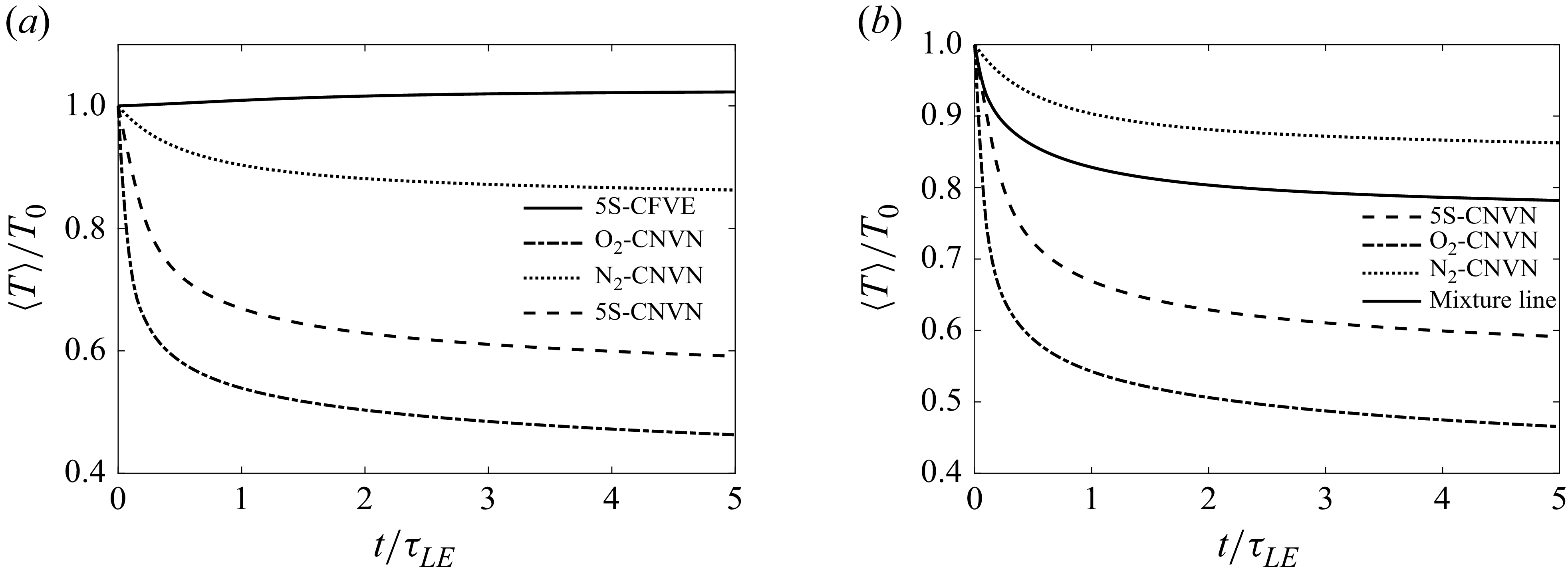
) are the major contributors in an air mixture; the behaviour of nitric oxide (NO) is excluded from this analysis. Therefore, we solely focus on the dynamics of nitrogen and oxygen molecules. Figure 5(a) shows the temporal evolution of mean temperature
 $\langle T \rangle$
across four simulation cases: 5S-CFVE,
 ${\textrm{O}}_2$
-CNVN,
 ${\textrm{N}}_2$
-CNVN and 5S-CNVN. Each plot is normalised by the initial temperature (
 $T_0$
). We observe that, except in the 5S-CFVE case where the mean temperature
 $(\langle T \rangle )$
shows a slight increase, all other cases show a monotonic decrease over time. Among these, the drop in mean temperature is maximum in the
 ${\textrm{O}}_2$
-CNVN case, with a substantial decrease of approximately
 $55\,\%$
compared with the initial value of
 $\langle T \rangle$
. The least decrease occurs in the
 ${\textrm{N}}_2$
-CNVN case, with a reduction of approximately
 $14\,\%$
. The decrease in the 5S-CNVN case is approximately
 $42\,\%$
, which lies between those observed in the
 ${\textrm{O}}_2$
-CNVN and
 ${\textrm{N}}_2$
-CNVN cases.
In the 5S-CFVE case, the observed increase in temperature
 $\langle T \rangle$
results from the conversion of kinetic energy into mean internal energy due to the processes of pressure dilatation and viscous dissipation. However, the temperature decrease in the
 ${\textrm{O}}_2$
-CNVN and
 ${\textrm{N}}_2$
-CNVN cases are primarily attributed to the endothermic dissociation of
 ${\textrm{N}}_2$
and
 ${\textrm{O}}_2$
molecules, respectively. This dissociation absorbs heat, leading to a reduction in overall temperature. Conversely, the overall drop in temperature in the 5S-CNVN case is attributable to the simultaneous occurrence of endothermic and exothermic reactions: the endothermic reactions absorb heat and tend to drop in temperature, while the exothermic reactions release heat, eventually offsetting the overall temperature drop observed in figure 5(a).
A more significant drop in temperature in the
 ${\textrm{O}}_2$
-CNVN case compared with the
 ${\textrm{N}}_2$
-CNVN case can be explained by the molecular properties and dissociation behaviours of oxygen and nitrogen molecules. Oxygen molecules (
 ${\textrm{O}}_2$
) have a lower bond dissociation energy than nitrogen molecules (
 ${\textrm{N}}_2$
), allowing them to dissociate more easily and at lower temperatures. This dissociation is an endothermic process in which heat is absorbed to break molecular bonds, leading to a greater reduction in temperature. In contrast, the dissociation rate for nitrogen molecules (
 ${\textrm{N}}_2$
) is slower due to the high energy required to break their stronger triple bonds. As a result, during the same period, nitrogen absorbs less heat from the environment compared with oxygen, leading to a slower rate of temperature decrease in the simulation
 ${\textrm{N}}_2$
-CNVN.
To examine whether the temperature drop observed in the 5S-CNVN case is merely a consequence of its intermediate composition or instead reflects the simultaneous effects of endothermic and exothermic reactions, we have conducted a mixture line analysis. The mixture line, shown in figure 5(b) as the mass-fraction-weighted average of the mean temperatures from the
 ${\textrm{N}}_2$
-CNVN and
 ${\textrm{O}}_2$
-CNVN cases using the instantaneous
 ${\textrm{N}}_2$
and
 ${\textrm{O}}_2$
mass fractions from the 5S-CNVN simulation, serves as a compositional benchmark. If the temperature evolution in 5S-CNVN were determined solely by the changing composition, the actual mean temperature curve would closely follow this mixture line. However, our results show that the mean temperature in the 5S-CNVN case is significantly lower than the mixture line prediction, despite having intermediate composition. This clear departure cannot be explained by composition alone, and is instead attributable to the competing effects of both endothermic and exothermic reactions, unique to the chemically reacting air mixture system.
(a) Temporal evolution of mean temperatures in the 5S-CFVE,
 ${\textrm{O}}_2$
-CNVN,
 ${\textrm{N}}_2$
-CNVN and 5S-CNVN cases. (b) Comparison of mean temperature evolution in the 5S-CNVN case with the mass-fraction-weighted mixture line constructed from
 ${\textrm{N}}_2$
-CNVN and
 ${\textrm{O}}_2$
-CNVN.

To provide evidence of the existence of both endothermic and exothermic processes in the 5S-CNVN simulation, we define the following quantity, which we call as the cumulative heat release (CHR) associated with the formation of a unit mass of the
 $s{\textrm{th}}$
species
 \begin{equation} {\textrm{CHR}}_s = -\int _0^{t}\langle h^0_{s}\,\dot {\omega }_s\rangle \,{\textrm d}t, \end{equation}
where
 $h^0_{s}$
is the formation enthalpy of species
 $s$
and
 $\dot {\omega }_s$
is its volume-averaged net source term of that species (production/destruction rate). A negative value of
 ${\textrm{CHR}}_s$
implies that the cumulative formation of that species up to time
 $t$
must have extracted heat from the mean flow (endothermic formation process). However, if
 ${\textrm{CHR}}_s$
has a positive value, it implies the opposite: the cumulative formation of that species up to time
 $t$
must have released heat into the mean flow (exothermic formation process). For diatomic species
 ${\textrm{N}}_2$
and
 ${\textrm{O}}_2$
, the formation enthalpy is zero, so
 ${\textrm{CHR}}_s$
will be identically zero at all times. Therefore, we need to focus on the cumulative heat release only on the other species in the mixture:
 ${\textrm{NO}}$
,
 ${\textrm{N}}$
and
 ${\textrm{O}}$
in the 5S-CNVN case, atomic nitrogen in the
 ${\textrm{N}}_2$
-CNVN simulation and atomic oxygen in the
 ${\textrm{O}}_2$
-CNVN case.
Table 5 presents the CHR (in
 ${\textrm{J m}}^{-3}$
) for each relevant species. These values are obtained by performing an integration of expression (4.1) over the time period
 $t=0$
to
 $t/\tau _{\textit{LE}}=5$
. We observe that in simulations
 ${\textrm{N}}_2$
-CNVN and
 ${\textrm{O}}_2$
-CNVN, only negative
 ${\textrm{CHR}}_s$
is observed. Thus, these simulations involve only endothermic processes. In contrast, the 5S-CNVN simulation has the simultaneous presence of both positive and negative
 ${\textrm{CHR}}_s$
. Thus, indeed, both exothermic and endothermic processes are active in the 5S-CNVN simulation. This makes the inherent energetics of the thermochemical relaxation process in a reacting air-mixture inherently different from the simple dissociating mixtures of the
 ${\textrm{N}}_2$
-CNVN and
 ${\textrm{O}}_2$
-CNVN cases.
Cumulative heat release (CHR in
 ${\textrm{J m}}^{-3}$
) for: NO, N and O in the 5S-CNVN case,
 ${\textrm{N}}$
in
 ${\textrm{N}}_2$
-CNVN, and
 ${\textrm{O}}$
in
 ${\textrm{O}}_2$
-CNVN.

Now, we discuss the vibrational relaxation process of nitrogen
 ${\textrm{N}}_2$
and oxygen
 ${\textrm{O}}_2$
molecules in different simulation cases. Figure 6 shows the temporal evolution of the mean temperature
 $\langle T \rangle$
, and the vibrational temperature of each molecule
 $\langle T_{V_m} \rangle$
for
 ${\textrm{O}}_2$
-CNVN,
 ${\textrm{N}}_2$
-CNVN and 5S-CNVN cases.
We observe a decrease in the mean temperature (
 $\langle T \rangle$
) and an increase in the vibrational temperature (
 $\langle T_{V_m} \rangle$
) across all cases, as shown in figure 6. These simultaneously occurring trends highlight the inherent tendency of the flow field to attain a state of vibrational equilibrium in accordance with (2.17). In the
 ${\textrm{O}}_2$
-CNVN case shown in figure 6(a), both temperatures attain equilibrium within one-fourth of an eddy-turnover time (
 $t/\tau _{\textit{LE}} = 0.25$
).
Figure 6(b) shows the temporal evolution of nitrogen molecules in the
 ${\textrm{N}}_2$
-CNVN case. In this case,
 $\langle T \rangle$
and
 $\langle T_{V_m} \rangle$
approach equilibrium by the end of the fourth eddy-turnover time (
 $t/\tau _{\textit{LE}} = 4$
). Figure 6(c) presents the vibrational relaxation process for
 ${\textrm{N}}_2$
and
 ${\textrm{O}}_2$
molecules in the chemically reacting air mixture (5S-CNVN) case. Here,
 ${\textrm{N}}_2$
reaches equilibrium by the end of
 $2.5$
eddy-turnover times, whereas
 ${\textrm{O}}_2$
achieves equilibrium at
 $4.0$
eddy-turnover times. Notably, the time required to achieve equilibrium of
 ${\textrm{O}}_2$
in the 5S-CNVN case is slower compared with the
 ${\textrm{O}}_2$
-CNVN case. However, the equilibration time of
 ${\textrm{N}}_2$
in the 5S-CNVN case is faster than that observed in the
 ${\textrm{N}}_2$
-CNVN case.
We wish to better understand the observation of figure 6. Plausibly, there are two broad reasons why the vibrational temperature of a diatomic molecule (
 ${\textrm{N}}_2$
or
 ${\textrm{O}}_2$
) will tend to equilibrate faster/slower in an air mixture (5S-CNVN) compared with other simulations like
 ${\textrm{O}}_2$
-CNVN and
 ${\textrm{N}}_2$
-CNVN. The first reason could be that (i) the vibrational relaxation time scale (
 $\langle \tau _{V_m} \rangle$
) of a diatomic molecule itself reduces in a chemically reacting air mixture, or alternatively, (ii) the vibrational relaxation process may be hastened merely by the fact that the mean temperature (
 $\langle T\rangle$
) itself drops at a faster rate enabling the vibrational temperature (
 $\langle T_{V_m} \rangle$
) to equilibrate faster.
Thermal relaxation of mean translational–rotational and mean vibrational temperatures in (a)
 ${\textrm{O}}_2$
-CNVN, (b)
 ${\textrm{N}}_2$
-CNVN and (c) 5S-CNVN cases.

In figure 7(a), we present the volume averaged vibrational relaxation times (
 $\langle \tau _{V_m} \rangle$
) for
 ${\textrm{O}}_2$
molecules in the
 ${\textrm{O}}_2$
-CNVN and 5S-CNVN cases. Despite having shorter relaxation times in the 5S-CNVN case, the oxygen molecules take longer to equilibrate than those in the
 ${\textrm{O}}_2$
-CNVN case, as shown in figure 6(c). This appears counterintuitive since shorter relaxation times typically imply faster equilibration. The explanation lies in the evolution of mixture temperature. As shown in figure 5(a), the mean temperature (
 $\langle T \rangle$
) in the 5S-CNVN case drops by approximately 42 % from its initial value, which is approximately 13 % less than the temperature drop observed in the
 ${\textrm{O}}_2$
-CNVN case. Consequently, the final mixture temperature in the 5S-CNVN case is higher, requiring the vibrational temperature of oxygen molecules (
 $\langle T_{V_{{\textrm{O}}_2}} \rangle$
) to increase further to reach equilibrium. This larger gap between
 $\langle T_{V_{{\textrm{O}}_2}} \rangle$
and
 $\langle T\rangle$
offsets the benefit of shorter relaxation times, leading to a slower overall equilibration. Thus, in the case of
 ${\textrm{O}}_2$
, only the second reason – the influence of mixture temperature – appears to govern the equilibration behaviour.
In contrast, figure 7(b) shows that the relaxation time for
 ${\textrm{N}}_2$
in the 5S-CNVN case is also shorter than in the
 ${\textrm{N}}_2$
-CNVN case. In this scenario, the expected trend holds true: the vibrational temperature of nitrogen molecules equilibrates faster in the 5S-CNVN case than in the
 ${\textrm{N}}_2$
-CNVN case, as seen in figure 6(c). This behaviour is consistent with the conventional understanding that shorter relaxation times promote faster vibrational equilibration. The difference again relates to how the mean temperature evolves. As illustrated in figure 5(a), the 5S-CNVN case sees a 42 % drop in mean temperature, substantially larger than the 14 % drop observed in the
 ${\textrm{N}}_2$
-CNVN case from initial temperature. As a result, the final mixture temperature in the 5S-CNVN case is much lower, allowing the vibrational temperature of nitrogen molecules (
 $\langle T_{V_{{\textrm{N}}_2}} \rangle$
) to match with the mixture temperature quickly. Here, both mechanisms – the reduced relaxation time and the larger drop in mixture temperature – act together to speed up the vibrational equilibration of
 ${\textrm{N}}_2$
molecules.
Temporal evolution of vibrational time scale of
 ${\textrm{O}}_2$
and
 ${\textrm{N}}_2$
molecules in
 ${\textrm{O}}_2$
-CNVN,
 ${\textrm{N}}_2$
-CNVN and 5S-CNVN simulation cases.

Next, we present the temporal evolution of the root-mean-square (r.m.s.) of the local temperature fluctuations (
 $\sqrt {\langle T' T' \rangle }$
) and vibrational temperature fluctuations (
 $\sqrt {\langle T^{\prime}_{V_m} T^{\prime}_{V_m} \rangle }$
) in figure 8. The r.m.s. values are normalised by the factor
 $(n-1)T_0M_t^2$
. These data correspond to the
 ${\textrm{O}}_2$
-CNVN,
 ${\textrm{N}}_2$
-CNVN and 5S-CNVN simulation cases.
In each case, the r.m.s. values of both the local and vibrational temperatures initially rise, reach a peak and then decay monotonically as turbulence evolves. In the
 ${\textrm{O}}_2$
-CNVN case, figure 8(a), a disparity is initially observed between the r.m.s. of the local and vibrational temperatures. However, this difference diminishes over time and nearly vanishes by the end of
 $2.5$
eddy-turnover times, indicating equilibration of local and vibrational temperature fluctuations. In contrast, the
 ${\textrm{N}}_2$
-CNVN case (figure 8
b) maintains a consistent disparity between
 $\sqrt {\langle T' T' \rangle }$
and
 $\sqrt {\langle T^{\prime}_{V_m} T^{\prime}_{V_m} \rangle }$
throughout the decay period.
Thermal relaxation of r.m.s. of translational–rotational and that of vibrational temperatures in (a)
 ${\textrm{O}}_2$
-CNVN, (b)
 ${\textrm{N}}_2$
-CNVN and (c) 5S-CNVN cases.

Figure 8(c) presents the temporal evolution of r.m.s. fluctuations of the mixture temperature, and that of the vibrational temperatures for nitrogen and oxygen molecules in the 5S-CNVN case. The disparity between the r.m.s. of translational–rotational and vibrational temperatures remains evident for both
 ${\textrm{O}}_2$
and
 ${\textrm{N}}_2$
throughout the simulation. Additionally, the peak values attained by both temperature fluctuations are relatively lower for
 ${\textrm{O}}_2$
and
 ${\textrm{N}}_2$
in the 5S-CNVN case when compared with their respective values in the
 ${\textrm{O}}_2$
-CNVN and
 ${\textrm{N}}_2$
-CNVN cases.
The above-mentioned study concludes that mean temperatures and mean vibrational temperatures achieve equilibrium after certain eddy turnover times in any non-equilibrium case. This equilibration period is delayed for oxygen molecules, whereas expedited for nitrogen molecules in the chemically reacting air mixture (5S-CNVN) case. However, there is a continuous disparity between the r.m.s. values of local and vibrational temperatures, specifically in the reacting air mixture.
4.2. Evolution of
${\textit{Re}}_{\lambda }$
,
$M_t$
and energy spectrum


In figure 9, we present the temporal evolution of the Taylor-scale Reynolds number (
 ${\textit{Re}}_\lambda$
) and the turbulent Mach number (
 $M_t$
) for all simulation cases. This figure shows that all simulation cases begin with identical initial values of
 ${\textit{Re}}_\lambda$
and
 $M_t$
, and exhibit nearly identical decay trends throughout the simulation period. Evidently, there is no direct significance influence of the thermochemical non-equilibrium processes on the decay of these quantities.
We acknowledge that our DNS are conducted at moderate Reynolds number (
 ${\textit{Re}}_{\lambda } = 30$
) and turbulent Mach number (
 $M_t = 0.3$
), which may be lower than those in practical hypersonic flows. While it is desirable to perform these simulations with higher values of these parameters, we are constrained by the limitations of our computational infrastructure. Nonetheless, our findings are still relevant for several reasons. First, the universality of small-scale turbulence statistics – such as intermittency, anomalous scaling and velocity gradient dynamics – is well established to emerge even at moderate Reynolds numbers. Previous studies (Schumacher, Sreenivasan & Yakhot Reference Schumacher, Sreenivasan and Yakhot2007; Yakhot & Donzis Reference Yakhot and Donzis2017) have demonstrated that the essential phenomenology and statistical features of small-scale turbulence are observable within the parameter ranges used in our simulations. Second, our choice of parameters is consistent with recent high-fidelity DNS studies on non-equilibrium turbulence by Kerkar & Ghosh (Reference Kerkar and Ghosh2024), which provide important benchmarks for turbulence model development and validation. Third, both our study and our recently published works have shown that essential interactions between turbulence and thermochemical non-equilibrium can be meaningfully captured and analysed at these accessible Reynolds and Mach numbers. While we do wish to caution against direct quantitative extrapolation of our results to practical hypersonic conditions, we believe that the insights gained from our study offer valuable physical understanding and high-fidelity reference data for modelling non-equilibrium turbulent flows.
Temporal evolution of (a) the Taylor-scale Reynolds number (
 ${\textit{Re}}_\lambda$
) and (b) the turbulent Mach number (
 $M_t$
) for the 5S-CNVN, 5S-CFVE,
 ${\textrm{N}}_2$
-CNVN and
 ${\textrm{O}}_2$
-CNVN simulation cases.

Next, we examine the kinetic energy spectrum,
 $E(\kappa )$
, expressed in Kolmogorov-compensated form,
 $E(\kappa )\kappa ^{5/3}\varepsilon ^{-2/3}$
, which is commonly used as a diagnostic of inertial-range energy transfer (Pope Reference Pope2000; Jiménez et al. Reference Jiménez, Wray, Saffman and Rogallo1993). Figure 10 presents the spectra at the initial instant (
 $t=0$
) and at a later time (
 $t/\tau _{\textit{LE}}=2.5$
) for all simulation cases. At
 $t=0$
, all spectra collapse exactly, reflecting the identical initial conditions imposed across the simulations. To further understand the differences observed in the dissipation range, we next examine the statistics of the velocity-gradient and pressure–Hessian tensors in § 4.3.
Temporal evolution of the kinetic energy spectrum expressed in Kolmogorov-compensated form,
 $E(\kappa )\kappa ^{5/3}\varepsilon ^{-2/3}$
, as a function of normalised wavenumber
 $\kappa\eta$
, shown at
 $t=0$
and
 $t/\tau _{\textit{LE}}=2.5$
for the 5S-CFVE,
 ${\textrm{O}}_2$
-CNVN,
 ${\textrm{N}}_2$
-CNVN and 5S-CNVN cases.

Temporal evolution of (a)
 $\varOmega ^{\prime 2}$
and (b)
 $\theta ^{\prime 2}$
in the 5S-CFVE,
 ${\textrm{O}}_2$
-CNVN,
 ${\textrm{N}}_2$
-CNVN and 5S-CNVN cases.

4.3. Influence of thermochemical non-equilibrium on the velocity gradient and the pressure-Hessian tensors
Motivated by these observations of the kinetic energy cascade, we proceed to examine the various turbulent processes – from spectral space to physical space – that govern the amplification of velocity gradients and the behaviour of pressure-Hessian tensors under different thermochemical non-equilibrium conditions.
Figure 11 presents the temporal evolution of the vortical and dilatational fluctuation intensities,
 $\varOmega ^{\prime 2}$
(3.8) and
 $\theta ^{\prime 2}$
(3.9), for the 5S-CFVE,
 ${\textrm{O}}_2$
-CNVN,
 ${\textrm{N}}_2$
-CNVN and 5S-CNVN simulation cases. In figure 11
a, the vortical fluctuations are normalised by their respective initial values,
 $\varOmega ^{\prime 2}(t=0)$
, such that all cases start from an identical reference state. All cases exhibit an initial growth followed by a decay of
 $\varOmega ^{\prime 2}$
, reflecting the combined effects of vortex stretching and viscous dissipation.
To further assess whether the observed differences in vortical fluctuations arise solely from the initial conditions, figure 11(b) shows the same quantity normalised by the enstrophy value at a later reference time,
 $t/\tau _{\textit{LE}}=2.0$
. With this normalisation, the curves do not collapse onto each other; instead, substantial differences persist across all cases, with deviations of up to approximately
 $45\,\%$
in the r.m.s. vorticity. This clearly demonstrates that the observed differences in the evolution of vortical fluctuations are not merely an artefact of the initial conditions. Rather, they indicate a continuous influence of thermochemical effects, with a systematic dependence on the Damköhler number.
Further, figure 11(c) shows the evolution of normalised dilatational fluctuations, (
 $\theta ^{\prime 2}/\varOmega _0^{\prime 2}$
), over time for the different simulation cases. It is evident that both vibrational and chemical non-equilibrium significantly influence the magnitude of dilatational fluctuations. The highest levels of
 $\theta ^{\prime 2}$
are observed in the 5S-CFVE case, where neither vibrational relaxation nor chemical reactions are active. In contrast, the lowest values occur in the 5S-CNVN case, which includes both vibrational and chemical non-equilibrium effects. The pure oxygen (
 ${\textrm{O}}_2$
-CNVN) case and the pure nitrogen (
 ${\textrm{N}}_2$
-CNVN) case exhibit intermediate behaviour.
In isotropic turbulent flows, the p.d.f. of
 $A_{\textit{ii}}$
typically features a single peak centred at zero (Sinha & Girimaji Reference Sinha and Girimaji2013). However, simulations initiating with higher turbulent Mach numbers exhibit a broader distribution, indicating a substantial presence of fluid elements with non-zero
 $A_{\textit{ii}}$
values, where
 $A_{\textit{ii}} \lt 0$
signifies contracting elements and
 $A_{\textit{ii}} \gt 0$
indicates expanding fluid elements. We choose the time
 $t/\tau _{{LE}} = 2.5$
as a representative instant to analyse the p.d.f.s of
 $A_{\textit{ii}}$
, computed from four simulation cases (5S-CFVE,
 ${\textrm{O}}_2$
-CNVN,
 ${\textrm{N}}_2$
-CNVN and 5S-CNVN). Similar trends are observed at other time instants as well, specifically at
 $t/\tau _{{LE}} = 1.5$
,
 $3.5$
and
 $4.5$
. To avoid repetition, additional figures for these times are not included. Figure 12 clearly shows that the presence of vibrational and chemical non-equilibrium in the flow field influences the distribution of
 $A_{\textit{ii}}$
. Notably, the p.d.f. is widest in the absence of these non-equilibrium effects (5S-CFVE case), and becomes narrower with the presence of vibrational and chemical effects. Among the
 ${\textrm{O}}_2$
-CNVN,
 ${\textrm{N}}_2$
-CNVN and 5S-CNVN cases, the
 ${\textrm{N}}_2$
-CNVN case shows the widest distribution, followed by
 ${\textrm{O}}_2$
-CNVN and 5S-CNVN. Consistent with the r.m.s. of dilatational fluctuation
 $(\theta ^{\prime 2})$
shown in figure 11(c), where the magnitude is highest in the 5S-CFVE case followed by the
 ${\textrm{N}}_2$
-CNVN,
 ${\textrm{O}}_2$
-CNVN and 5S-CNVN cases, the distribution of
 $A_{\textit{ii}}$
follow the same pattern.
Probability distribution function of
 $A_{\textit{ii}}$
. Influence of thermochemical non-equilibrium in the 5S-CFVE,
 ${\textrm{O}}_2$
-CNVN,
 ${\textrm{N}}_2$
-CNVN and 5S-CNVN cases.

To further understand the behaviour observed in figures 11(a), 11(c) and 12, we directly refer to the evolution equation for the velocity gradient tensor (2.32) and extract its contracted form,
 \begin{equation} \frac {\textrm D}{{\textrm D}t}(A_{\textit{ij}}A_{\textit{ij}}) = \underbrace {-A_{\textit{ik}}A_{\textit{kj}}A_{\textit{ij}}}_{\text{Inertial mechanism}} - \underbrace {P_{\textit{ij}}A_{\textit{ij}}}_{\text{Pressure mechanism}} - \underbrace {\varGamma A_{\textit{ij}}}_{\text{Viscous mechanism}}. \end{equation}
This equation represents the evolution of the square of the magnitude of the velocity gradient tensor following a local fluid element. We focus our analysis entirely on the first two mechanisms appearing in (4.2). The contribution of viscous processes is not examined in this study. Our attention is restricted to identifying the influence of the inertial (
 $-A_{\textit{ik}}A_{\textit{kj}}A_{\textit{ij}}$
) and pressure (
 $-P_{\textit{ij}}A_{\textit{ij}}$
) mechanisms in magnifying the strength of the velocity gradient tensor
 $(A_{\textit{ij}}A_{\textit{ij}})$
in compressible flows.
We present the temporal evolution of the normalised velocity gradient magnitude,
 $\langle A_{\textit{ij}}A_{\textit{ij}}\rangle /\langle A_{\textit{ij}}A_{\textit{ij}}\rangle _{t=0}$
, for all four simulation cases, as shown in figure 13. In each case, the normalised quantity shows an initial increase, reaching a peak value within the first eddy turnover time, and subsequently decreases monotonically as turbulence decays. Among the cases, the
 ${\textrm{O}}_2$
-CNVN simulation shows the highest sustained values of
 $\langle A_{\textit{ij}}A_{\textit{ij}}\rangle /\langle A_{\textit{ij}}A_{\textit{ij}}\rangle _{t=0}$
throughout the simulation, followed by the 5S-CNVN, 5S-CFVE and
 ${\textrm{N}}_2$
-CNVN cases. This ordering is consistent with the trends observed for the vortical fluctuations shown in figure 11(a).
Temporal evolution of the normalised velocity gradient magnitude
 $\langle A_{\textit{ij}}A_{\textit{ij}}\rangle /\langle A_{\textit{ij}}A_{\textit{ij}}\rangle _{t=0}$
in the 5S-CFVE,
 ${\textrm{O}}_2$
-CNVN,
 ${\textrm{N}}_2$
-CNVN and 5S-CNVN cases.

In incompressible turbulence, it is observed that the predominant tendency of the inertial triadic mechanism is to amplify the magnitude of the velocity gradient tensor. However, the act of the pressure-Hessian tensor, in incompressible turbulence, has been identified to be opposite: the pressure-Hessian tensor tends to counteract the amplifying action of the pressure-related mechanisms (see Chevillard & Meneveau Reference Chevillard and Meneveau2006; Meneveau Reference Meneveau2011). However, the counteracting action is not enough to completely cancel out the amplifying tendency of the inertial mechanism, and thus, overall, in incompressible turbulence, the velocity gradient magnitude still tends to grow with time. At the other extreme, Bikkani & Girimaji (Reference Bikkani and Girimaji2007) has performed an analysis of the velocity gradient dynamics in the ‘pressure-released’ limit of Burgers turbulence. In this limit, the pressure-Hessian tensor is non-existent, altogether. They demonstrate that in this limit of flow behaviour, indeed, the rate of amplification of the velocity gradient tensor is further enhanced compared with that in incompressible turbulence. In the background of these findings, we now provide a plausible explanation of the behaviour observed in figures 11(a) and 13.
We conjecture that in our simulations, the presence of thermochemical non-equilibrium processes causes a moderation of the counteracting action of the pressure-Hessian tensor. This moderation, in turn, leads to a higher impact of the already existing amplifying action of the inertial mechanism on the right-hand side of (4.2). To verify this conjecture, in figure 14, we show the p.d.f. of the magnitude of the pressure-Hessian tensor
 $(\sqrt {P_{mn}P_{mn}})$
, normalised by (
 $A_{\textit{ij}}A_{\textit{ij}}$
) at
 $t=0$
. Figure 14 shows the p.d.f. of
 $log(\psi )$
, where
 $\psi =\sqrt {P_{mn}P_{mn}}/(A_{\textit{ij}}A_{\textit{ij}})_{t=0}$
, across different simulation cases at a representative time instant of
 $t/\tau _{\textit{LE}}=2.5$
. Indeed, we observe that in different simulations, there is a relative shift in the distribution towards the left. Specifically, the distribution of the p.d.f.s in chemically reacting air-mixture case shifts towards lower values of
 ${\textrm{log}}(\psi )$
compared with the equilibrium case. This indicates that the thermochemical non-equilibrium processes weaken the strength of the pressure-Hessian tensor. Further, the trend in the reduction of the magnitude of the pressure-Hessian tensor in figure 14 is fairly in line with the trend by which the magnitude of the velocity gradient tensor increases in figures 11(a) and 13. We observe a similar trend in the p.d.f.s at other time instants (
 $t/\tau _{\textit{LE}}=1.5, 3.5$
and
 $4.5$
) as well.
Probability distribution function of
 $\psi =\sqrt {P_{mn}P_{mn}}/(A_{\textit{ij}}A_{\textit{ij}})_{t=0}$
in the 5S-CFVE,
 ${\textrm{O}}_2$
-CNVN,
 ${\textrm{N}}_2$
-CNVN and 5S-CNVN cases.

Proceeding further along this line of explanation, figure 15 shows the temporal evolution of the r.m.s. of pressure fluctuations in various simulations. A clear trend can be observed, which appears to correlate with the drop in temperature shown in figure 5(a). As discussed in § 4.1, there is a significant disparity in the extent to which the mean temperature decreases in the different simulations. This disparity in temperature drop – whether the flow field becomes hotter or colder – seems to lead to a corresponding disparity in the strength of pressure fluctuations, as governed by the equation of state for the constituent gases. The observed suppression of pressure fluctuations in a colder mixture, in turn, suppresses the strength of the pressure-Hessian tensor itself. A suppressed pressure-Hessian tensor then loses its ability to counteract the inherent action of the inertial mechanism described in (4.2). This suppression eventually leads to the disparity observed in
 $\langle \varOmega _i\varOmega _i\rangle$
and
 $\left \langle {A}_{\textit{ij}}A_{\textit{ij}}\right \rangle$
, as shown in figures 11(a) and 13.
Temporal variation in the r.m.s. of pressure fluctuation in 5S-CFVE,
 ${\textrm{O}}_2$
-CNVN,
 ${\textrm{N}}_2$
-CNVN and 5S-CNVN cases.

4.4. Behaviour of vibrational and chemical mechanisms in the evolution of the modified pressure-Hessian tensor
In this section, we make an attempt to understand the relationship between the disparity in the magnitude of the pressure-Hessian as observed in figure 14 and the specific thermochemical non-equilibrium mechanisms instrumental in the evolution equation of (2.35).
Danish, Sinha & Srinivasan (Reference Danish, Sinha and Srinivasan2014) employ a DNS database of isotropic compressible turbulence to examine the impact of inertial, conduction and viscous mechanisms on the evolution of the pressure-Hessian tensor
 $(P_{\textit{ij}})$
. Their investigation excludes specific considerations of vibrational relaxation and chemical reactions in the flow field. They reduce the complex tensorial form of
 $P_{\textit{ij}}$
to a simpler scalar equation,
 $ {\textrm D}/{{\textrm D}t}(P_{\textit{ij}}P_{\textit{ij}})$
, converting the tensor mechanisms into contracted scalar forms and then examine the relative importance of each mechanism in the simplified scalar equation. Following a similar methodology, we first contract (2.35) with
 $P_{\textit{ij}}$
to derive its scalar form as
 \begin{align} & \frac {1}{2}\ \frac {{\textrm D}}{{\textrm D}t}\left (P_{\textit{ij}}P_{\textit{ij}}\right )\ = \underbrace {\left (-A_{\textit{kj}}P_{\textit{ik}}-A_{\textit{ki}}P_{\textit{kj}}-(n-1)A_{\textit{kk}}P_{\textit{ij}}\right )P_{\textit{ij}}}_{(I')}\nonumber \\ &\quad \underbrace {-\frac {np}{\rho }\left (\frac {\partial ^2A_{\textit{kk}}}{\partial x_i\partial x_j}-\frac {1}{\rho }\frac {\partial A_{\textit{kk}}}{\partial x_i}\frac {\ \partial \rho }{\partial x_j}\right )P_{\textit{ij}}}_{(II')}\nonumber \\ &\quad \underbrace {-\left [\frac {(n-1)}{\rho } \frac {\partial A_{\textit{kk}}}{\partial x_j}\ \frac {\partial p}{\partial x_i} +\frac {n}{\rho } \frac {\partial A_{\textit{kk}}}{\partial x_i}\ \frac {\partial p}{\partial x_j} + \frac {1}{\rho } \frac {\partial A_{\textit{ki}}}{\partial x_j}\ \frac {\partial p}{\partial x_k} \right ] P_{\textit{ij}}}_{(III')}\nonumber \\ &\quad \underbrace {-(n-1)\frac {\partial }{\partial x_j} \left [ \frac {1}{\rho } \frac {\partial }{\partial x_i} \left ( \sum _{m=1}^{nd} \left ( \frac {\rho _m e_{V_m}^*}{\tau _{\textit{Vm}}} - \frac {\rho _m e_{V_m}}{\tau _{\textit{Vm}}} \right ) \right ) \right ]P_{\textit{ij}}}_{(IV')}\nonumber \\ &\quad \underbrace {-(n-1) \frac {\partial }{\partial x_j} \left [ \frac {1}{\rho } \frac {\partial }{\partial x_i} \left ( \sum _{m=1}^{nd} \dot {\omega }_m e_{V_m} + \sum _{s=1}^{ns} h_s^0 \dot {\omega }_s \right ) \right ]P_{\textit{ij}}}_{(V')}.\nonumber \\ & \underbrace {+(n-1) \frac {\partial }{\partial x_j} \! \left [ \frac {1}{\rho } \frac {\partial }{\partial x_i}\! \left ( \frac {\partial }{\partial x_k}\! \left ( \sum _{m=1}^{nd} \rho _m u_{\textit{mk}}^D e_{V_m} - \sum _{s=1}^{ns} \rho _s u_{sk}^D h_s\! \right ) + \sum _{s=1}^{ns} h_s^0 \frac {\partial }{\partial x_k} \big(\rho _s u_{sk}^D\big)\! \right )\! \right ]P_{\textit{ij}}}_{({\textit{VI}}^{\prime})}. \end{align}
In (4.3), mechanisms
 $I^{\prime}{-}{\textit{III}}^{\prime}$
are the scalar counterparts of the inertial mechanisms I–III from (2.35). The mechanism
 ${\textit{IV}}^{\prime}$
corresponds to the scalar version of mechanism IV, and it specifically represents the vibrational mechanism. Similarly, mechanisms
 $V^{\prime}$
and
 ${\textit{VI}}^{\prime}$
are the scalar forms of mechanisms V and VI, which are classified as chemical mechanisms. Now, our goal is to examine the behaviour of these scalar mechanisms across different simulation cases.
To examine the influence of thermochemical non-equilibrium on the flow dynamics, we define a function
 $f_1$
in (4.4) that quantifies the relative contribution of vibrational and chemical mechanisms compared with inertial mechanisms in the evolution of the pressure-Hessian tensor:
 \begin{equation} f_1 = \frac {|{\textit{IV}}^{\prime}+V^{\kern-1.5pt\prime}+{\textit{VI}}^{\prime}|}{|I^{\kern-1.5pt\prime}+{\textit{II}}^{\prime}+{\textit{III}}^{\prime}| + |{\textit{IV}}^{\prime}+V^{\kern-1.5pt\prime}+{\textit{VI}}^{\prime}|} , \end{equation}
where the numerator represents the combined effects of vibrational and chemical contributions, and the denominator includes all relevant contributions, inertial, vibrational and chemical. By definition, the value of
 $f_1$
ranges from 0 to 1, indicating the degree to which the vibrational and chemical mechanisms together influence the evolution of the pressure-Hessian tensor. A value of
 $f_1\rightarrow 0$
implies that the inertial mechanisms completely control the flow without the influence of the vibrational and chemical effects. In contrast,
 $f_1\rightarrow 1$
indicates that the vibrational and chemical mechanisms dominate over the inertial effects on the flow dynamics following small fluid elements.
Figure 16(a) shows the temporal evolution of the spatial average
 $\langle |f_1| \rangle$
for the
 ${\textrm{O}}_2$
-CNVN,
 ${\textrm{N}}_2$
-CNVN and 5S-CNVN cases. This function quantifies the relative contribution of vibrational and chemical mechanisms compared with inertial effects in the evolution of the pressure-Hessian tensor. In all three cases, thermochemical non-equilibrium mechanisms play a substantial role, with
 $\langle |f_1| \rangle$
remaining significantly above zero throughout the simulation.
The evolution of
 $\langle |f_1| \rangle$
shows two distinct phases. Initially, there is a sharp rise from near zero to a peak value, showing the influence of vibrational relaxation and chemical reactions over inertial effects in the initial phase. This is followed by a gradual decrease in function
 $\langle |f_1| \rangle$
as the system approaches a steady state.
Although the qualitative behaviour of
 $\langle |f_1| \rangle$
is similar across the three simulations, their magnitudes differ significantly. The
 ${\textrm{O}}_2$
-CNVN case shows the strongest influence of thermochemical non-equilibrium, with a peak value of approximately 0.3 and an asymptotic value of 0.25. In contrast, the
 ${\textrm{N}}_2$
-CNVN case shows the weakest influence, with peak and asymptotic values around 0.05 and 0.04, respectively. The 5S-CNVN case falls between the two, with a peak of 0.2 and an asymptotic value of 0.1. These trends suggest that simulations based solely on oxygen may overestimate the influence of vibrational and chemical non-equilibrium effects on the evolution of the pressure-Hessian equation compared with the chemically reacting air mixture case, while nitrogen-only simulations may underestimate it. Eventually, all three cases approach steady-state values, with the 5S-CNVN case consistently situated between the
 ${\textrm{O}}_2$
-CNVN and
 ${\textrm{N}}_2$
-CNVN cases. The analysis of function
 $\langle |f_1| \rangle$
clearly reveals the significant role of vibrational and chemical mechanisms in shaping the behaviour of the pressure-Hessian tensor (2.35) and, consequently, the velocity gradient tensor (2.32) in chemically reacting air mixture.
Temporal evolution of (a)
 $\langle |f_1|\rangle$
, (b)
 $\langle |f_2|\rangle$
and (c)
 $\langle |f_3|\rangle$
in the
 ${\textrm{O}}_2$
-CNVN,
 ${\textrm{N}}_2$
-CNVN and 5S-CNVN cases.

Now, we wish to examine the relative contribution of vibrational versus chemical non-equilibrium in the evolution of the pressure-Hessian equation. Among the overall thermochemical non-equilibrium mechanisms, two distinct contributions are present: vibrational and chemical mechanisms. To examine the relative influence of the vibrational mechanism (Mechanism IV) compared with the chemical mechanisms (Mechanisms V and VI) in the evolution of the pressure-Hessian tensor, we define a second function,
 $f_2$
, as
 \begin{equation} f_2 = \frac {|{\textit{IV}}^{\prime}|}{|{\textit{IV}}^{\prime}| + |V^{\prime}+{\textit{VI}}^{\prime}|}. \end{equation}
Figure 16(b) presents the temporal evolution of the function
 $\langle |f_2|\rangle$
for the
 ${\textrm{O}}_2$
-CNVN,
 ${\textrm{N}}_2$
-CNVN and 5S-CNVN simulation cases. In the
 ${\textrm{N}}_2$
-CNVN case,
 $\langle |f_2|\rangle$
exhibits high initial values just after
 $t=0$
, indicative of a dominant vibrational non-equilibrium mechanism at early times. Subsequently,
 $\langle |f_2|\rangle$
decreases monotonically throughout the simulation duration. In contrast, for the
 ${\textrm{O}}_2$
-CNVN and 5S-CNVN cases,
 $\langle |f_2|\rangle$
is initially small and rapidly decreases to near-zero values within a very short time, remaining almost constant thereafter. The observed behaviour of
 $\langle |f_2|\rangle$
across these simulation cases can be explained based on their respective vibrational relaxation characteristics. The notably higher initial value of
 $\langle |f_2|\rangle$
in the
 ${\textrm{N}}_2$
-CNVN case can be attributed to the inherently longer vibrational relaxation time of nitrogen (
 ${\textrm{N}}_2$
). Figure 6(b) clearly shows this delay in reaching equilibrium (see § 4), where the large initial difference between mean translational–rotational and mean vibrational temperatures persists for approximately the first two eddy turnover times. This delayed equilibration maintains the vibrational mechanisms active in the flow field during the initial phase of the simulation. In contrast, the sharp decrease of
 $\langle |f_2|\rangle$
observed in the
 ${\textrm{O}}_2$
-CNVN and 5S-CNVN cases during the same period is plausibly due to the relatively faster vibrational relaxation processes in pure oxygen (
 ${\textrm{O}}_2$
-CNVN) and the reactive air mixture represented by 5S-CNVN as shown in figures 6(a) and 6(b), respectively. In these cases, rapid equilibration of vibrational energies to local temperatures diminishes the influence of vibrational non-equilibrium relative to chemical non-equilibrium, thereby sharply reducing
 $\langle |f_2|\rangle$
within the first half of the eddy turnover time. The analysis of the function
 $\langle |f_2| \rangle$
concludes that the contribution of vibrational mechanisms compared with chemical mechanisms is dominant only in the
 ${\textrm{N}}_2$
-CNVN case, but is negligible in the
 ${\textrm{O}}_2$
-CNVN and 5S-CNVN cases.
We now shift our focus exclusively to the chemical mechanisms within the pressure-Hessian (2.35). There are two distinct chemical mechanisms at play: Mechanism V, which represents the production of various species due to chemical reactions, and Mechanism VI, which describes species diffusion effects in the flow field. To evaluate the relative contributions of these two mechanisms, we define another quantity
 $f_3$
:
 \begin{equation} f_3 = \frac {|V^{\prime}|}{|V^{\prime}|+|{\textit{VI}}^{\prime}|}. \end{equation}
Clearly,
 $\langle |f_3|\rangle$
quantifies the influence of species production mechanisms (Mechanism V) relative to the diffusion-driven mechanisms (Mechanism VI) in the evolution of the pressure-Hessian tensor.
Figure 16(c) presents the temporal evolution of the function
 $\langle |f_3| \rangle$
for the
 ${\textrm{O}}_2$
-CNVN,
 ${\textrm{N}}_2$
-CNVN and 5S-CNVN simulation cases. In all three cases,
 $\langle |f_3| \rangle$
initially increases, indicating a rapid rise in the relative influence of species production mechanisms compared with species diffusion mechanisms. After this initial transient period, the function stabilises to nearly constant values. Specifically, the 5S-CNVN case shows the highest stabilised value, clearly highlighting the dominant role of production-driven chemical mechanisms in the reacting air mixture.
The higher magnitude of
 $\langle |f_3|\rangle$
observed in the 5S-CNVN case can be attributed to the interactions among five different chemical species (N
 $_2$
, O
 $_2$
, NO, N and O) present in 5S-CNVN mixture. The simultaneous presence of these species significantly enhances the occurrence of the production of molecules, increasing the relative contribution of these mechanisms compared with pure
 ${\textrm{O}}_2$
and pure
 ${\textrm{N}}_2$
cases. The
 ${\textrm{N}}_2$
-CNVN case exhibits the lowest stabilised value, indicating a comparatively stronger contribution from diffusion-driven chemical mechanisms. This behaviour is consistent with nitrogen molecules being lighter and hence being more diffusive than oxygen molecules. This plausibly enhances the role of species diffusion relative to species production in the
 ${\textrm{N}}_2$
-dominated environment as represented by the lower value of
 $\langle |f_3|\rangle$
in figure 16(c).
While the present findings reveal clear trends in the relative dominance of production versus diffusion-driven chemical mechanisms across different non-equilibrium cases, it is important to acknowledge a modelling limitation inherent to our study. We model mass diffusion for each species using a modified Fick’s law with a species-specific time and temperature-dependent diffusion coefficient. While this approach captures differences in diffusivity among species, it does not include the full cross-diffusion effects present in a complete multi-component model. Therefore, our analysis of
 $\langle |f_3|\rangle$
reflects differential diffusion to some extent, but remains an approximation. Nonetheless, our principal findings regarding the relative roles of production and diffusion-driven mechanisms remain robust within the present simulation framework, and our results clearly highlight the amplified impact of production-driven mechanisms in multi-species environments.
It should also be noted that at the initial time (
 $t=0$
), both the vibrational and chemical source terms are physically inactive. Consequently,
 $\langle |f_2|\rangle$
and
 $\langle |f_3|\rangle$
are not defined initially, and their temporal evolution is presented only for
 $t/\tau _{\textit{LE}} \gt 0$
so that all reported values correspond to physically meaningful quantities.
The analysis of the
 ${\textrm{O}}_2$
-CNVN,
 ${\textrm{N}}_2$
-CNVN and 5S-CNVN simulation cases demonstrates how vibrational and chemical non-equilibrium mechanisms affect the pressure-Hessian tensor and, consequently, the evolution of the velocity gradient tensor in turbulent flows. In pure-nitrogen environments, the effects of vibrational mechanisms are more significant due to longer relaxation times, but these effects quickly diminish in pure-oxygen and chemically reacting air mixture environments. Species production-driven chemical mechanisms significantly influence the pressure-Hessian tensor in the 5S-CNVN case, indicating that chemical reactions change density and pressure gradients by altering the local species composition.
5. Significance and implications of this work
The dynamics of small-scale velocity gradients is deemed to be a means to understand the evolution of various turbulence processes like energy cascade, intermittency, material element deformation and mixing (Meneveau Reference Meneveau2011). Even though some researchers have recently reported limited measurements related to the velocity gradient tensors (Xu, Pumir & Bodenschatz Reference Xu, Pumir and Bodenschatz2011), extensive experimental observations of this tensor are rare even today. This limitation arises due to the difficulty in simultaneously measuring the gradients of a vector in all three directions. Direct numerical simulations of flow fields do offer an opportunity to access extensive Eulerian velocity fields, based on which the velocity gradient tensor information can be constructed numerically to an acceptable level of accuracy. However, following the pioneering work of Vieillefosse (Reference Vieillefosse1982) and Cantwell (Reference Cantwell1992), several researchers (Ashurst et al. Reference Ashurst, Kerstein, Kerr and Gibson1987; Girimaji & Pope Reference Girimaji and Pope1990; Li & Meneveau Reference Li and Meneveau2005; Chevillard & Meneveau Reference Chevillard and Meneveau2006) have emphasised the need to develop an alternate approach to study the dynamics of velocity gradients in turbulent flows. This approach employs an autonomous set of closed ordinary differential equations to track the evolution of the velocity gradient tensor in a Lagrangian sense (following the motion of a small local fluid element). Such an approach is not only computationally more viable than performing direct numerical simulations of turbulent flows, but is also deemed to be more intuitive, as all changes following the motion of an identified material fluid element can be directly monitored. Further, such a closed set of equations developed for the evolution of velocity gradients in a turbulent flow field has been shown to be directly useful for the Lagrangian p.d.f. methods of turbulence (Pope Reference Pope1994).
Owing to these advantages, many advanced models for the evolution of the velocity gradient tensor have been developed for incompressible flows and some compressible flows as well. The key to developing such models is: (i) to adequately understand the physics of the pressure-Hessian tensor; and subsequently, (ii) to mathematically model these physical processes – as in (2.32) – from which a closed equation for the velocity gradient tensor can be obtained.
In the context of incompressible turbulence, the most advanced and widely accepted phenomenological model is that of Chevillard & Meneveau (Reference Chevillard and Meneveau2006). This is called the recent fluid deformation (RFD) closure model. Indeed, this model has been shown to reproduce several statistical features of incompressible turbulence. Recently, Shikha, Srivastava & Sinha (Reference Shikha, Srivastava and Sinha2024) has taken a step forward and developed a machine-learning based model for the pressure-Hessian tensor and demonstrated an improved performance of the model even over the RFD model.
Despite the considerable success of the RFD model of Chevillard & Meneveau (Reference Chevillard and Meneveau2006) or the ML-based model of Shikha et al. (Reference Shikha, Srivastava and Sinha2024), these models are inherently unsuitable for compressible flows. These models inherently assume: (i) the velocity gradient to be traceless and (ii) model the pressure-Hessian tensor in terms of the velocity field itself. Quite differently, in compressible turbulence, pressure evolves thermodynamically through the flow density and temperature. Thus, any modelling attempt solely in terms of the velocity field of the flow is not physically sensible. Accordingly, Sinha & Girimaji (Reference Sinha and Girimaji2009) and Danish et al. (Reference Danish, Sinha and Srinivasan2014) included an evolution equation (another set of ordinary differential equations) for the pressure-Hessian tensor, as well. This equation was obtained using the evolution equations of density and temperature (energy equation). While their models of the velocity gradient tensor do capture many features of the compressible turbulence (Reynolds number and Mach number effects), no model exists for a compressible flow field wherein both vibrational and chemical non-equilibrium exist (hypersonic flow fields). The current work is a step forward in that direction.
Prior studies on compressible velocity gradient modelling have been limited to either equilibrium assumptions (Sinha & Girimaji Reference Sinha and Girimaji2013; Danish et al. Reference Danish, Suman and Srinivasan2016) or simplified single-species models (Martın & Candler Reference Martın and Candler1999; Neville et al. Reference Neville, Nompelis, Subbareddy and Candler2014; Kerkar & Ghosh Reference Kerkar and Ghosh2024), leaving significant gaps in our understanding of realistic air mixtures under thermochemical non-equilibrium conditions. While our earlier work (Srivastava & Sinha Reference Srivastava and Sinha2025) established a theoretical framework for vibrational and chemical non-equilibrium, it was restricted to a pure oxygen case with only endothermic dissociation reactions. The present study extends this framework by carrying out DNS of turbulence in a five-species, 17-reaction model that includes both endothermic and exothermic reactions. This approach enables us to capture the thermochemical behaviour of atmospheric air under conditions relevant to hypersonic and atmospheric re-entry flows.
The motivation behind generating the DNS database presented in this work is to identify, isolate and understand how vibrational and chemical non-equilibrium processes influence the evolution of the pressure-Hessian tensor. The analysis performed herein – particularly in § 4.4 – demonstrates that, despite the presence of numerous unclosed terms in the pressure-Hessian evolution equation, it is possible to develop a reasonable model by focusing on the most dominant mechanism in (2.35). Although the modelling aspect is beyond the scope of the present manuscript, it will be the primary focus of our future work. The utility of the current study is to provide the foundation based on which a mathematically closed evolution equation of the pressure-Hessian tensor, which can be applied to hypersonic flow conditions, will be developed.
6. Conclusions
The primary aim of this study is to enhance our understanding of the pressure-Hessian tensor and its impact on the velocity gradient tensor in high-temperature compressible turbulence. This research specifically focuses on the combined effects of vibrational and chemical non-equilibrium in high-speed flows relevant to scenarios such as atmospheric re-entry of spacecraft and cruise flights of hypersonic vehicles through an earth-like atmosphere.
In this work, we use the exact evolution equations for the pressure-Hessian tensor and the velocity gradient tensor, including the physics of chemical and vibrational non-equilibrium in a five-species air mixture. This approach leads to the identification of new unclosed mechanisms in the evolution equation of the pressure-Hessian tensor. Using the hy2Foam solver on the OpenFOAM platform, we perform several direct numerical simulation (DNS) studies of isotropic compressible decaying turbulence. A five-species air mixture consisting of molecular nitrogen (N
 $_{2}$
), molecular oxygen (O
 $_{2}$
), nitric oxide (NO), atomic nitrogen (N) and atomic oxygen (O) along with a set of 17 chemical reactions is used in the study. The reacting air model accounts for the energy exchange between the translational–rotational and the vibrational modes using the classical Landau–Teller model. The vibrational relaxation time is computed from the Millikan-White and Park formulations. Additionally, detailed finite-rate chemistry mechanisms are implemented to capture species-specific reactions and their impact on turbulence.
The specific findings of this study are the following.
-
(i) The analysis of the temporal evolution of the mean temperature shows the significant role of vibrational and chemical non-equilibrium processes in the flow field. For the reacting air mixture (5S-CNVN) case, the mean temperature monotonically reduces. However, this reduction lies intermediate between that observed in the
${\textrm{O}}_2$
-CNVN and
${\textrm{N}}_2$
-CNVN cases. Specifically, the
${\textrm{O}}_2$
-CNVN case experiences the largest temperature drop due to the more dissociating nature of oxygen molecules. Conversely, the
${\textrm{N}}_2$
-CNVN case exhibits the smallest temperature drop, as nitrogen molecules require significantly more energy for dissociation. The intermediate behaviour in the 5S-CNVN case is attributed to both endothermic and exothermic reactions. In contrast to these non-equilibrium cases, the equilibrium case 5S-CFVE, which has a non-reacting air mixture, exhibits merely a small temperature increase, primarily caused by the conversion of kinetic energy into internal energy through viscous dissipation and pressure dilatation processes. Any non-equilibrium effect is absent in this case. -
(ii) This study highlights significant differences in achieving the vibrational equilibrium of oxygen and nitrogen molecules within the chemically reacting air mixture environment. For oxygen molecules, the time required to achieve equilibrium is delayed in the reacting air mixture case compared with the pure oxygen case. This slower equilibration happens despite the fact that the vibrational relaxation time for oxygen molecules is smaller in the reactive air environment (5S-CNVN) compared with the pure oxygen (
${\textrm{O}}_2$
-CNVN) case. The delayed equilibration is primarily due to the larger initial difference between the vibrational temperature of oxygen molecules (
$\langle T_{V_{{\textrm{O}}_2}} \rangle$
) and the overall mean temperature (
$\langle T\rangle$
) in the 5S-CNVN case. In contrast, nitrogen molecules equilibrate faster in the 5S-CNVN case compared with the pure nitrogen (
${\textrm{N}}_2$
-CNVN) case. This enhanced equilibration occurs because the overall mixture temperature in the multi-species case drops more significantly, helping the vibrational temperature of nitrogen molecules (
$\langle T_{V_{{\textrm{N}}_2}} \rangle$
) quickly reach equilibrium. Additionally, shorter vibrational relaxation times of nitrogen molecules in the 5S-CNVN case further contribute to achieving faster equilibration relative to the
${\textrm{N}}_2$
-CNVN case. -
(iii) The magnitude of vortical fluctuations increases in the chemically reacting air mixture case compared with a non-reacting air mixture. However, the levels of vortical fluctuations in a reacting air mixture are intermediate between those observed for the pure oxygen and pure nitrogen cases. In contrast, dilatational fluctuations decrease in a reacting air mixture compared with a non-reacting air mixture.
-
(iv) The p.d.f. of the trace (
$A_{\textit{ii}}$
) of the velocity gradient tensor indicates that vibrational and chemical non-equilibrium conditions in the chemically reacting air mixture notably narrow the distribution, indicating a reduction in the proportion of fluid elements experiencing extreme contraction or expansion events compared with a non-reacting air mixture as well as compared with flows where only
${\textrm{N}}_2$
and
${\textrm{O}}_2$
dissociation reactions are considered. -
(v) The strength of the pressure-Hessian tensor relative to the velocity gradient tensor is reduced in a chemically reacting air mixture compared with a non-reacting air mixture.
-
(vi) Evolution of the pressure-Hessian tensor in the chemically reacting air mixture is significantly influenced by thermochemical non-equilibrium mechanisms (vibrational and chemical), contributing approximately 12 % to the overall dynamics compared with the inertial mechanisms active in the evolution equation of the pressure-Hessian tensor. However, within these thermochemical non-equilibrium processes, the role of vibrational mechanisms, although noticeable in the pure nitrogen case, becomes negligible in the reactive air mixture. Among the chemical non-equilibrium mechanisms, we find that the mechanism related to the production of chemical species is more prominent than the chemical non-equilibrium mechanism arising due to the species diffusion process.


It is important to emphasise that the present DNS studies were conducted at moderate Reynolds number (
 ${\textit{Re}}_\lambda = 30$
) and turbulent Mach number (
 $M_t = 0.3$
), which are lower than those typically encountered in practical hypersonic flows. This limitation arises from the limited computational resources available to the authors. However, several factors support the continued relevance of our findings. The universality of small-scale turbulence statistics and the essential mechanisms of turbulence interactions with thermochemical non-equilibrium are well known to emerge at these Reynolds and Mach numbers, as established in prior literature. Our results, therefore, provide valuable physical insight and high-fidelity reference data, which can serve as benchmarks for turbulence model development in non-equilibrium high-speed flows. We hope that future work – enabled by advances in computational power – will extend these investigations to even higher Reynolds and Mach numbers, further bridging the existing gap up to the practical hypersonic conditions.
In conclusion, these results demonstrate the significant role of a chemically reacting air-mixture on the dynamics of velocity gradient and the pressure-Hessian tensor in high-temperature compressible turbulence. The findings are expected to make important contributions to the development of closure models for pressure-Hessian tensors in chemically reactive and vibrationally excited flows. These findings not only improve our understanding of chemical and vibrational non-equilibrium processes on turbulence dynamics, but can also possibly be leveraged to arrive at improved turbulence closure models for hypersonic turbulent flows.
Acknowledgements
The computing resources required for this work have been made available by the High-Performance Computing Center (HPC), Indian Institute of Technology, Delhi, India.
Funding
This work has been financially supported by the Science and Engineering Research Board (SERB), Department of Science and Technology, Government of India, through Project No. CRG/2022/002378.
Declaration of interests
The authors report no conflict of interest.
Appendix A
A.1. Viscosity coefficients
Viscosity coefficients (
 $A_{B,s}$
,
 $B_{B,s}$
,
 $C_{B,s}$
) for each species are provided in table 6 (Blottner et al. Reference Blottner, Johnson and Ellis1971).
Blottner correlation coefficients
 $A_{B,s}$
,
 $B_{B,s}$
and
 $C_{B,s}$
for the calculation of species-specific viscosity used in (2.8).

A.2. Relaxation time data
Coefficients
 $A$
and
 $B$
used in (2.21) for computing the relaxation times
 $\tau _{\textit{m-s}}^{\textit{MW}}$
are given in table 7 (Park Reference Park1993).
Relaxation coefficients
 $A$
and
 $B$
used in (2.21).

A.3. Species thermochemical properties
Table 8 presents the thermochemical data used in our work for each chemical species. For each species
 $s$
, the table lists the molecular weight
 $M_s$
, the standard enthalpy of formation at 298 K (
 $ h^\circ _s$
) and the characteristic vibrational temperature (
 $\theta _{V,s}$
). These data are essential for accurately modelling and simulating chemical reactions within the solver.
Species thermochemical properties.

A.4. Chemical model parameters
Parameters needed for the five-species chemical model of Park (Reference Park1989) used in (2.28)–(2.30) are provided in table 9.