1. Introduction
Multi-robot path planning is a fundamental problem in multi-mobile robot systems. It aims to enable multiple robots to perform cooperative navigation and task execution in complex environments. In recent years, with the rapid development of unmanned systems, extensive research has been conducted in this area. Significant progress has been achieved, particularly in point-to-point path planning under dynamic and uncertain environments.
For example, in perception-limited environments, adaptive collision avoidance strategies have been developed for unmanned surface vehicles (USVs) by incorporating dynamic priority mechanisms and multi-agent reinforcement learning [Reference Yin and Xiang1]. In addition, some studies adopt distributed reinforcement learning frameworks to jointly optimize target assignment and path planning in multi-USV systems, thereby improving task completion efficiency and system safety [Reference Yin and Xiang2]. Furthermore, for collaborative tasks in complex environments, recent work has considered energy constraints and heterogeneous system characteristics, leading to multi-objective optimization approaches for cooperative path planning [Reference Yin and Xiang3].
However, most of these studies focus on point-to-point path planning. Their goal is to guide robots to specific target locations rather than to systematically traverse the entire environment. In this context, multi-robot coverage path planning (MCPP) has attracted increasing attention.
MCPP is a key application in multi-mobile robot systems, aiming to enable multiple robots to collaborate in avoiding obstacles while minimizing the time required to cover the free area in a map [Reference Galceran and Carreras4]. MCPP is widely applied in various indoor and outdoor scenarios, such as robotic vacuum cleaners [Reference Bormann, Jordan, Hampp and Hägele5], drone search and rescue operations [Reference Collins, Ghassemi, Esfahani, Doermann, Dantu and Chowdhury6], and agricultural harvesters [Reference Arab, Spisser and Essert7]. The spanning tree coverage (STC) [Reference Gabriely and Rimon8] algorithm, as a classical single-robot coverage path planning method, has been widely extended to MCPP research.
The core performance metric of MCPP is coverage time, defined as the time required by the last robot to complete the coverage task. Coverage time depends on both the path length and the number of turns in the robot paths [Reference Almadhoun, Taha, Seneviratne and Zweiri9]. While most studies target either metric independently, few address the joint optimization of both.
MCPP algorithms that aim to reduce path length can be classified into two categories based on whether size division is performed: size division-based methods and non-size division-based methods. The first category [Reference Kapoutsis, Chatzichristofis and Kosmatopoulos10, Reference Idir and Renzaglia11, Reference Baras and Dasygenis12, Reference Apostolidis, Kapoutsis, Kapoutsis and Kosmatopoulos13] divides the free area into several equal-sized subareas to ensure the minimal path length for each robot. The second category constructs a spanning tree to obtain a closed path, which is then assigned to multiple robots [Reference Agmon, Hazon and Kaminka14, Reference Zheng, Jain, Koenig and Kempe15, Reference Tang, Sun and Zhang16]. Due to overlapping coverage in the paths, the path length of the second category is generally longer than that of the first category. However, neither of these two categories considers the impact of robot turns on coverage time.
TMSTC* (Turn-minimizing Multi-robot Spanning Tree Coverage*) [Reference Lu, Zeng, Tang, Lam and Wen17] exhibits state-of-the-art (SOTA) performance compared to other algorithms by minimizing path turns. However, since the TMSTC* algorithm does not perform size division, its path length is not minimized.
In addition to coverage time, another key metric for MCPP is computation time, especially in large-scale maps. However, the computation time required by the aforementioned methods on large-scale maps is prohibitively high for practical applications.
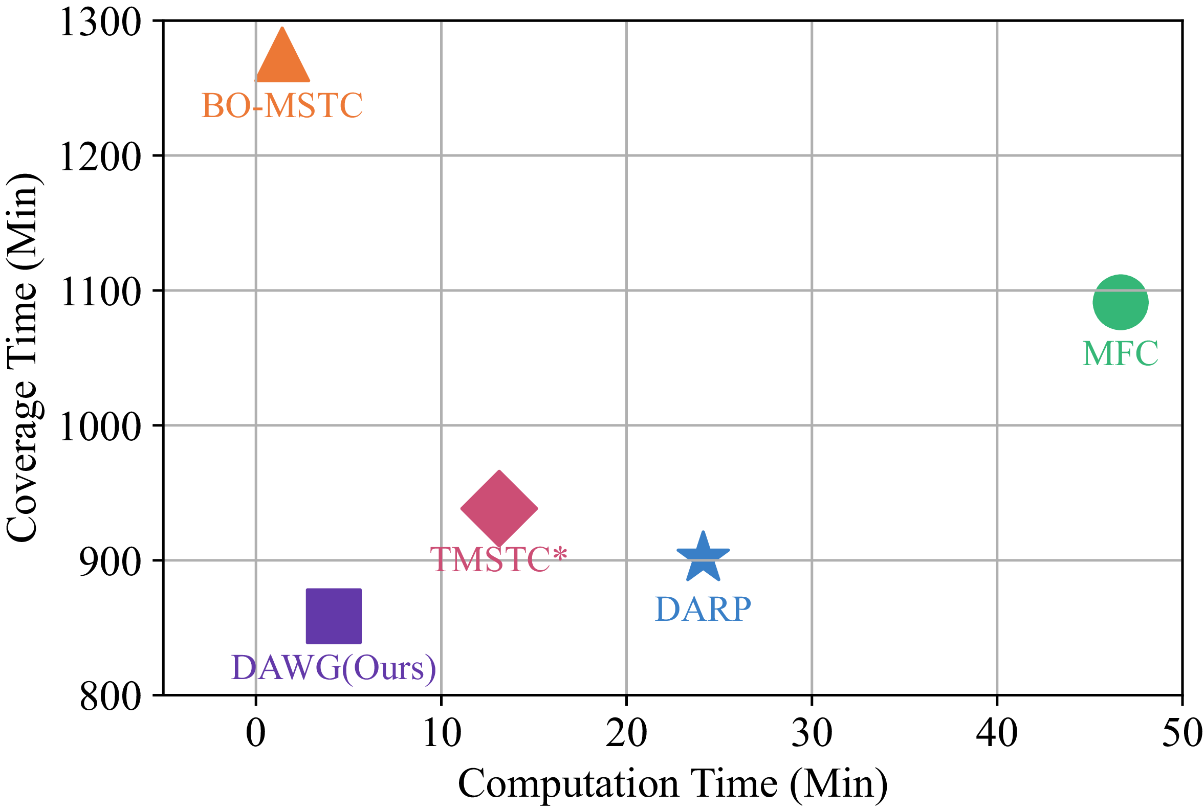
The performance comparison of our proposed DAWG algorithm with four existing algorithms: TMSTC* [Reference Lu, Zeng, Tang, Lam and Wen17], DARP (Divide Areas based on Robots Initial Positions) [Reference Kapoutsis, Chatzichristofis and Kosmatopoulos10], BO-MSTC (Backtracking-Multi-robot Spanning Tree Coverage) [Reference Agmon, Hazon and Kaminka14], and MFC (Multi-robot Forest Coverage) [Reference Zheng, Jain, Koenig and Kempe15], where all methods are evaluated on the same
 $512 \times 512$
map.

To address above issues, we propose the DAWG (Divide Areas based on area Growing [Reference Adams and Bischof18] via wavefront Propagation [Reference Zelinsky, Jarvis, Byrne and Yuta19]) algorithm, which can equally divides free area and minimizes path turn counts. Compared to existing methods, our approach not only achieves shorter coverage times but also reduces computation time, as shown in Figure 1. Our contributions are summarized as follows:
-
• We draw on the ideas of area growing and wavefront propagation to achieve an equal division of free area while ensuring the connectivity of each subarea. As a result, the path length is minimized, and computation time is kept low. We also propose a greedy method to minimize the number of bricks, achieving only a 3% increase in turn counts compared to TMSTC*, while reducing computation time by 81%. Additionally, by adjusting the distance metric used in wavefront propagation, we optimized the shapes of the subareas, further reducing turn counts.
-
• The proposed DAWG algorithm achieves the minimum path length while ensuring near-optimal turn counts. The overall coverage time of this algorithm outperforms SOTA algorithms, while its computation time remains at a low level, as shown in Figure 1.
-
• We observe that existing MCPP algorithms exhibit unstable computation times (e.g., computation times exceeding a specified limit, defined in this letter as no solution) when faced with large-scale map diversity. In contrast, the proposed DAWG algorithm always finds a feasible solution for all 24 different instances.
2. Related work
The core idea of MCPP is to divide and allocate the coverage tasks of the entire map among multiple robots, enabling them to collaboratively complete the coverage within the shortest possible time [Reference Tan, Mohd-Mokhtar and Arshad20]. The coverage time of MCPP is determined by the last robot to finish and depends on both the path length and the number of turns.
The STC [Reference Gabriely and Rimon8] is a classical single-robot CPP algorithm, and many existing MCPP methods have been extended based on it. These methods either focus solely on optimizing path length or exclusively on minimizing the number of turns, resulting in a notable lack of research that comprehensively addresses both aspects.
To reduce path length, MCPP algorithms can be categorized into two types based on whether size balancing is considered: size division-based methods and non-size division-based methods. Among the first category, DARP (Divide Areas based on Robots Initial Positions) [Reference Kapoutsis, Chatzichristofis and Kosmatopoulos10] (which partitions the area based on the initial positions of the robots) assigns each STC node to the nearest robot and iteratively adjusts the assignment to achieve equal-sized subareas. However, subsequent studies based on DARP [Reference Idir and Renzaglia11, Reference Baras and Dasygenis12] have shown that in maps with complex obstacle distributions, when the initial positions of robots are concentrated, the DARP may fail to ensure the connectivity of each robot’s subarea. Forcing subarea connectivity in such cases can result in redundant coverage, thereby increasing the path length. Among the second category, BO-MSTC (Backtracking-Multi-robot Spanning Tree Coverage) [Reference Agmon, Hazon and Kaminka14] algorithm treats the single-robot coverage path planned by the STC algorithm as a ring and divides the ring based on the initial positions of the robots to obtain coverage paths for multiple robots. Zheng et al. introduced MFC (Multi-robot Forest Coverage) [Reference Zheng, Jain, Koenig and Kempe15], whose core idea is to construct subtrees with similar weights and assign them to multiple robots. Tang et al. proposed MSTC* [Reference Tang, Sun and Zhang16], which uses a greedy strategy to address the imbalance in the ring division in BO-MSTC. However, both categories of studies have overlooked the minimization of the number of turns in the path.
To reduce the number of turns, Vandermeulen et al. proposed a checkerboard-style decomposition of the free space into multiple rectangular cells and applied an iterative heuristic to adjust their orientations [Reference Vandermeulen, Groß and Kolling21]. However, this method is limited in applicability as it cannot handle non-rectilinear environments effectively. Ramesh et al. introduced the OARP (Optimal Axis-Parallel Rank Partitioning) method, which minimizes the number of axis-parallel coverage lines by formulating the problem as a linear program (LP) [Reference Ramesh, Imeson, Fidan and Smith22]. However, the LP-based method is computationally expensive for large-scale environments, which limits its practicality. TMSTC* [Reference Lu, Zeng, Tang, Lam and Wen17] transforms the problem of minimizing turns into dividing the free area into the fewest number of bricks and then solving the maximum independent set of a bipartite graph to determine the minimum turns. Although TMSTC* achieves SOTA performance, its path length remains suboptimal.
In recent years, research on large-scale MCPP has begun to move beyond traditional small-scale experimental settings. For example, refs. [Reference Tang, Mao and Ma23] and [Reference Tang and Ma24] investigate large-scale grid-based coverage strategies from the perspectives of path conflict resolution and local search optimization, respectively. However, most existing MCPP methods are still primarily evaluated in small-scale scenarios such as household cleaning or indoor service environments. This creates a clear gap with real-world applications, including large public-space cleaning, warehouse logistics, and city-scale UAV inspection. In this context, it is necessary to systematically evaluate the computational efficiency and scalability of different algorithms on large-scale maps to better reflect their practical performance.
Traditional grid-based methods usually assume that the grid size matches the robot size. A grid cell is considered covered when the robot center passes through its center. However, in practical applications, grid cells may be smaller than the robot body. This makes it difficult for robots to navigate narrow areas, which reduces overall coverage performance. A straightforward solution is to reduce the robot size. However, this often leads to lower coverage efficiency.
To balance coverage completeness and efficiency, Samarakoon et al. [Reference Samarakoon, Muthugala and Kalimuthu25] proposed a size-adaptive robot model. The robot can dynamically adjust its size according to environmental constraints. It maintains a larger size in open areas to improve efficiency, while shrinking in narrow regions to ensure accessibility. In addition, Samarakoon et al. [Reference Samarakoon, Muthugala, Kalimuthu, Chandrasekaran and Elara26] proposed an online path planning method based on a Glasius neural network for such adaptive robots. This method enables real-time motion adaptation in dynamic environments. However, these methods are still mostly at the prototype stage. Their applicability in real large-scale systems has not yet been fully validated.
Recently, energy-aware and terrain-aware coverage path planning has received increasing attention. In these methods, robot motion is not only evaluated by geometric metrics such as path length but also by energy-related factors and environmental characteristics. EA-OSPGB (Energy Activity-Obstacle and Start Point Guidance and Backtracking mechanisms) [Reference Xu, Diao, Li, Liu, Zhang, Ye and Nie27] introduces an energy activity (EA) function to guide multi-robot coverage in unknown environments. The algorithm constructs a local raster activity value function to evaluate coverage decisions and incorporates a terrain-based backtracking mechanism to improve exploration efficiency. This mechanism enables robots to escape so-called “dead zones” during online exploration and reduces redundant backtracking paths caused by environmental uncertainty. Experimental results demonstrate that considering energy activity and terrain factors can effectively reduce both path length and turning cost in dynamic environments.
However, EA-OSPGB is fundamentally an online reactive coverage framework. Its decision-making process relies on real-time environmental feedback and energy activity evaluation, which leads to dynamic path adaptation during execution. While this improves adaptability in unknown environments, it may also introduce additional computational overhead and complex coordination behavior in large-scale scenarios.
In contrast, the method proposed in this paper, DAWG, does not rely on energy-driven reactive decision-making or terrain-dependent backtracking mechanisms. Instead, it adopts an offline deterministic decomposition strategy, where the coverage problem is first decomposed into balanced and connected subareas, followed by STC-based path construction within each subarea. This structural design allows DAWG to decouple partitioning and path optimization, enabling efficient global planning with significantly reduced computational cost.
Therefore, this letter adopts equal-size division to minimize path length and addresses the long computation time of TMSTC* on large-scale maps while maintaining a similar number of turns. Next, the algorithm design is presented in Section 4.
3. Preliminaries & motivation
3.1. MCPP problem definition
As illustrated in Figure 2(a), in the MCPP algorithm based on STC, assume that the robot’s coverage tool has a width of
 $ d$
, and the map is discretized into square grid cells with a width of
 $ 2d$
. Each grid cell, composed of four small square grid cells with a width of
 $ d$
, is either completely free or entirely occupied by obstacles. This dual-scale grid division enables the construction of two graphs: the coverage graph
 $ G$
and the spanning tree graph
 $ H$
. Specifically, the center of each small grid cell is taken as a coverage node, and edges are established between adjacent coverage nodes to form the coverage graph
 $ G$
. Similarly, the center of each grid cell is taken as a spanning tree node, and edges between adjacent spanning tree nodes form the spanning tree graph
 $ H$
.
Multi-robot coverage path planning using our method. (a) Coverage graph
 $G$
and spanning graph
 $H$
. (b) Division of the free area among robots, with initial positions marked by stars. (c) Coverage paths of the robots shown in different colors.

As shown in Figure 2(c), by executing the STC algorithm on the spanning tree graph
 $ H$
, the coverage paths
 $ \Pi _i$
for each robot can be obtained, where each path is generated by traversing around the corresponding spanning tree (hereafter referred to as the STC path). Therefore, the optimization goal of MCPP is to find a set of coverage paths such that the maximum coverage time is minimized:
 \begin{equation} \arg \min _{\{\Pi _i\}} \left ( \max _{1 \leq i \leq K} \left ( T_{\text{Cover}_i} \right ) \right ) \end{equation}
where
 $T_{\text{Cover}_i}$
is the coverage time of
 $\Pi _i$
.
3.2. MCPP problem analysis
In MCPP, the coverage time is influenced by both the path length and the number of turns. To reduce the coverage time, this work simultaneously optimizes both factors. On the one hand, the STC path
 $ \Pi _i$
of robot
 $ i$
has a length of
 $ S_i \times 4d$
, where
 $ S_i$
denotes the number of spanning tree nodes in the subarea assigned to robot
 $ i$
, which can also be regarded as the number of grid cells in that subarea. According to Eq. (1), dividing the free space into subareas with equal size helps minimize the maximum path length, thereby reducing the overall coverage time. On the other hand, further reducing the number of turns in each subarea can also effectively shorten the time required for individual robots to complete their tasks. Based on this analysis, the following two subsections present the strategy for equal-size subarea division and the construction of minimal-turn spanning trees, respectively.
3.2.1. Minimization of STC path length
Given the fixed number of spanning tree nodes in the free space, it is equally divided into
 $K$
subareas, where
 $K$
denotes the number of robots. Each subarea has an approximate size
 $S_i$
. The STC algorithm is then applied within each subarea, which helps balance the path lengths of all robots. Additionally, these
 $ K$
subareas should remain connected, and each robot’s initial position
 $ X_i$
is located within its corresponding subarea
 $ A_i$
. To avoid time waste caused by overlapping coverage, these subareas should ideally be non-overlapping. Therefore, the optimization objectives and constraints for size division are as follows:
 \begin{equation} \begin{aligned} \min \, & \max (S_1, S_2, \dots, S_K) \\ \text{s.t.} \quad & A_i \cap A_j = \emptyset, \quad \forall \, i \neq j, \\ & \mathrm{Connectivity}(A_i) = 1, \quad \forall \, i \in \{1, 2, \ldots, K\}, \\ & \mathbf{X}_i \in A_i, \quad \forall \, i \in \{1, 2, \ldots, K\}. \end{aligned} \end{equation}
Eq. (2), specifically the second constraint, ensures that each subarea
 $A_i$
assigned to a robot satisfies the following connectivity requirement. Since the robot is only allowed to move in four directions (up, down, left, and right), the 4-neighborhood is adopted as the basis for defining connectivity. Specifically, the grid cells in
 $A_i$
are regarded as nodes in a graph. If two cells satisfy the 4-neighborhood relationship, an edge is defined between them. Based on this definition,
 $A_i$
can be decomposed into several connected subsets under 4-neighborhood connectivity, that is, 4-connected components. The subarea
 $A_i$
is considered connected if and only if the number of 4-connected components is equal to one. Otherwise, it is regarded as disconnected. Therefore, the connectivity constraint can be formulated as:
 \begin{equation*} \text{Connectivity}(A_i) = \begin{cases} 1, & \text{if } N_{\text{comp}}(A_i) = 1 \\ 0, & \text{otherwise} \end{cases} \end{equation*}
where
 $N_{\text{comp}}(A_i)$
denotes the number of 4-connected components in subarea
 $A_i$
.
As a representative study on size division, the DARP algorithm transforms the problem of equally dividing the area into a clustering problem. However, the DARP algorithm exhibits three main limitations: it disregards the number of turns in the path while optimizing coverage time; it incurs significant computation time in large-scale maps; and it is sensitive to the initial distribution of robot positions, which can cause the algorithm to enter an infinite loop.
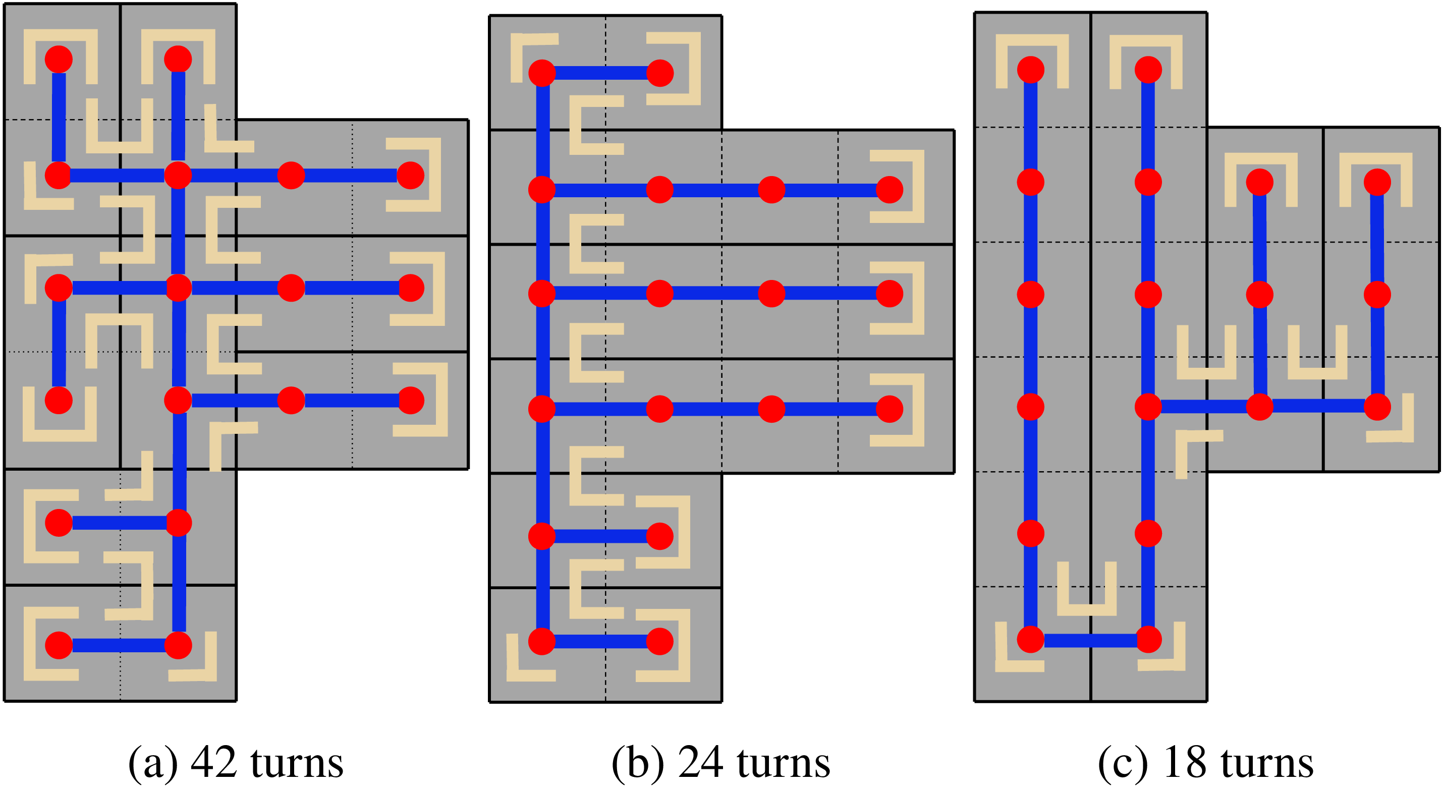
Comparison of turn counts (highlighted in beige, each representing a 90-degree turn) across different spanning tree constructions. Dashed lines divide the free space into grid cells, while solid lines divide it into bricks. Three spanning tree construction strategies: random, greedy, and TMSTC*, correspond to 9 bricks in (a), 6 bricks in (b), and 4 bricks in (c).

3.2.2. Minimization of STC path turns
The concept of brick was proposed in ref. [Reference Lu, Zeng, Tang, Lam and Wen17], where it is defined as a regular rectangular strip formed by merging multiple grid cells along either the horizontal or vertical direction, with a fixed width or height of
 $2D$
. A brick can alternatively be regarded as a segment of the spanning tree
 $ T$
, consisting of multiple nodes aligned in the same direction. Since the STC path only turns at the two endpoints of each brick and at the junctions between different bricks, a smaller number of bricks within the spanning tree
 $T$
generally leads to fewer turns in the corresponding STC path. As shown in Figure 3, for a given spanning tree graph H, different spanning tree construction strategies have a significant impact on the number of turns in the robot’s coverage path. According to ref. [Reference Lu, Zeng, Tang, Lam and Wen17], the problem of minimizing the number of turns can be equivalently transformed into minimizing the number of bricks
 $ B_i$
contained in the spanning tree
 $ T$
:
 \begin{equation} \begin{aligned} \min \, & \| B_1, B_2, \ldots, B_m \| \\ \text{s.t.} \quad & B_1 \cup B_2 \cup \cdots \cup B_m = H, \\ & B_i \cap B_j = \emptyset, \quad \forall \, i, j \in \{1, 2, \ldots, m\}, \, i \neq j. \end{aligned} \end{equation}
TMSTC* algorithm further transforms the problem of minimizing the number of bricks into solving the maximum independent set problem in a bipartite graph. Although TMSTC* achieves the best results so far in minimizing the number of turns, it does not divide the area, leaving room for improvement in reducing path length. Furthermore, the computation time of TMSTC* in large-scale maps also limits its practicality.
3.3. Motivation
In practical applications, robots cannot maintain a constant speed throughout the entire process. This is because turning introduces additional time cost. To simplify the problem, the following assumptions are made for the robot’s coverage process. First, the robot decelerates and accelerates with constant acceleration before and after turning. Second, when changing direction, the robot must reduce its linear velocity to zero and then perform a
 $90^\circ$
in-place rotation with a constant angular velocity. Under these assumptions, as shown in Eq. (5), both the path length and the number of turns should be optimized to reduce the overall coverage time.
Since the simultaneous optimization of path length and the number of turns is an NP-hard problem, this letter simplifies the problem into two sequential steps: generating equal-sized subareas, followed by constructing a minimal-turn spanning tree within each subarea. It should be noted that this simplification yields an approximate solution rather than the theoretical global optimum. Due to the high computational cost of the TMSTC* algorithm in the spanning tree construction phase, we propose a greedy strategy that significantly reduces the computation time while maintaining a comparable number of turns.
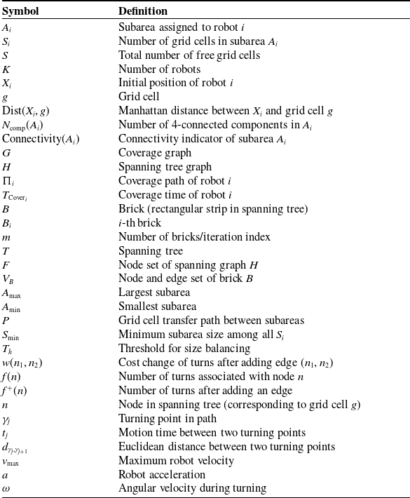
Summary of symbols and variable definitions used in this paper.

Table I. Long description
Panel A: Table listing symbols and their definitions used in a paper on robot coverage processes. The table includes columns for Symbol and Definition. Symbols include variables related to subareas, grid cells, robots, distances, components, graphs, trees, paths, times, bricks, nodes, edges, velocities, and accelerations. Definitions provide detailed explanations for each symbol.
To improve readability and ensure consistency of notation throughout the paper, we summarize the main symbols and variables used in this work in Table I. The table provides unified definitions for all key notations appearing in the main text, algorithms, and mathematical formulations. Symbols that are not explicitly defined in the main text are intentionally excluded to avoid ambiguity.
4. Our algorithm
In this section, we propose the DAWG algorithm, which aims to optimize the coverage time by simultaneously reducing the path length and the number of turns, while achieving a shorter computation time compared to existing SOTA algorithms.
4.1. Connectivity-assured equal-size division
The size division process of the DARP algorithm assigns each grid cell to the nearest robot based on distance. However, since the division of each grid cell is done independently, DARP may fail to ensure the connectivity of the subarea assigned to robot
 $ i$
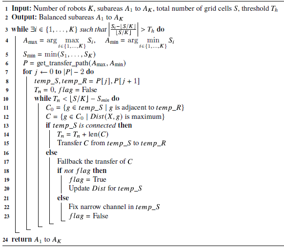
(Figure 4(a)). Differing from DARP, we draw inspiration from the area growing method in image segmentation [Reference Adams and Bischof18] and the wavefront propagation method [Reference Zelinsky, Jarvis, Byrne and Yuta19] and gradually expand the boundaries of subareas through area growing to naturally maintain the connectivity of subareas during the division process (Figure 4(a)). Algorithm1 summarizes the pseudocode of the proposed algorithm.
4.1.1. The process of grid cell transfer between adjacent subareas
Figure 5 illustrates the process of grid cell transfer between two adjacent subareas, aiming to equalize their sizes. Algorithm1.
Comparison of subarea connectivity between the DARP algorithm and the proposed DAWG algorithm. (a) Subareas are not connected. (b) Subareas are connected.

Figure 4. Long description
Panel A: A diagram showing subareas that are not connected. The diagram features various colored regions separated by black lines, with stars marking specific points within some regions. Panel B: A diagram showing subareas that are connected. Similar to Panel A, this diagram features various colored regions separated by black lines, with stars marking specific points within some regions.
The process of grid cell transfer between adjacent subareas of two robots until the free area is equally divided.

As shown in Figure 5(a), based on the Manhattan distance metric, the initial positions of the robots, denoted as
 $ X_1, X_2, \dots, X_K$
, are used as seed points to perform a Voronoi partition over the full map. Each grid cell
 $ g$
is assigned to the subarea corresponding to the robot
 $ i$
for which the Manhattan distance
 $ \text{Dist}(X_i, g)$
is the smallest, where
 $ \text{Dist}(X_i, g)$
denotes the Manhattan distance between the robot’s initial position
 $ X_i$
and the grid cell
 $ g$
. Initially, the sizes of subareas
 $ A_0$
and
 $ A_1$
are 18 and 75, respectively.
To balance the sizes among subareas, we first identify the subarea with the largest size, denoted as
 $A_{\text{max}}$
, and the one with the smallest size, denoted as
 $A_{\text{min}}$
. Before introducing the transfer process, we define the adjacency relationship between subareas. Two subareas
 $A_i$
and
 $A_j$
(
 $i \neq j$
) are defined as adjacent if there exists at least one pair of grid cells
 $g \in A_i$
and
 $g' \in A_j$
that satisfy the 4-neighborhood relationship. In other words, the two subareas share at least one pair of 4-neighboring boundary cells. Based on this definition, a valid grid cell transfer path is constructed on the adjacency graph of subareas using the function
 $P_{A_{\text{max}} \rightarrow A_{\text{min}}} = \texttt{get_transfer_path}(A_{\text{max}, A_{\text{min}}})$
. For notational simplicity, we omit the dependency on
 $(A_{\text{max}}, A_{\text{min}})$
and use
 $P$
to denote the corresponding transfer path in the remainder of this paper. Since grid cells can only be transferred directly between adjacent subareas, if
 $A_{\text{max}}$
and
 $A_{\text{min}}$
are not adjacent, the function returns a sequence of intermediate subareas that forms a connected path between them.
For example, let
 $P = [1,2,3,4]$
, where subareas 1 and 4 correspond to
 $A_{\text{max}}$
and
 $A_{\text{min}}$
, respectively. In this case, the transfer from subarea 1 to subarea 4 must pass through subareas 2 and 3, and any two consecutive subareas in
 $P$
are adjacent according to the above definition. Therefore, the grid cell transfer path is
 $A_1\,(\text{sender}) \rightarrow A_0\,(\text{receiver})$
, and the number of transferred grid cells is
 $\left \lfloor \frac {S}{K} \right \rfloor - S_{0} = 28$
. Here,
 $S$
denotes the total number of free grid cells (i.e., excluding obstacle cells), where
 $S = \sum _{i=1}^{K} S_i$
, and
 $i \in \{1,\dots, K\}$
. Therefore,
 $\left \lfloor S/K \right \rfloor$
represents the discretized average number of free grid cells assigned to each subarea, corresponding to the desired balanced coverage load.
As shown in Figure 5(b), the part of the sender area adjacent to the receiver contains four grid cells. If these grid cells are all assigned to the receiver at once, it may lead to two issues: the sender area becoming disconnected, or the sender’s initial position being assigned to the receiver. To avoid these problems, the appropriate approach is to gradually assign the grid cells farthest from the sender’s initial position to the receiver. This approach is based on the observation that, when the sender area expands outward, the farthest grid cells are the last ones added; conversely, when the sender area shrinks, the farthest grid cells should be the first to be removed.
As shown in Figure 5(c), during the first iteration, two grid cells were successfully transferred from the sender to the receiver.
It is important to note that, in theory, the wavefront distance within the sender area should be updated in each iteration (i.e., grid cells outside the sender area are treated as obstacles); otherwise, the situation shown in Figure 5(e) may occur, where the sender becomes disconnected from the receiver. However, repeatedly updating the wavefront distance incurs a significant computational cost, especially in large-scale maps. To reduce the computational time, as shown in Figure 5(b)–(e), the wavefront distance is not updated after each iteration.
When the sender area becomes disconnected, as shown in Figure 5(e)–(g), the division process rolls back to the previous round and updates the wavefront distance. As shown in Figure 5(h), the division process continues while the imbalance among subareas remains significant. Specifically, the algorithm continues if the relative deviation of any subarea size from the average value exceeds a predefined threshold
 $T_h$
, as described in Step 1 of Algorithm1. The process terminates only when the sizes of all subareas are sufficiently close to the average value.
Here,
 $T_h$
represents a tolerance threshold that controls the maximum allowable relative imbalance between each subarea and the ideal average size. Formally, the continuation condition is defined as:
 \begin{equation*} \left |\frac {S_i - \lfloor S/K \rfloor }{\lfloor S/K \rfloor }\right | \gt T_h, \end{equation*}
where
 $S_i$
denotes the number of grid cells in subarea
 $A_i$
, and
 $\lfloor S/K \rfloor$
is the discretized average number of grid cells per subarea.
Equal-size division

Algorithm 1 Long description
An equation representing an algorithm for dividing subareas among robots. The algorithm starts with inputs including the number of robots K, subareas A1 to AK, total number of grid cells S, and a threshold Th. The output is balanced subareas A1 to AK. The algorithm uses a while loop to check if the size of any subarea exceeds the threshold. It identifies the subareas with the maximum and minimum sizes and calculates the minimum size among all subareas. It then retrieves a transfer path and iterates over this path. Within this iteration, it identifies adjacent grid cells and those with maximum distance. If the temporary subarea is connected, it updates the transfer count and transfers cells. If not, it falls back on the transfer and updates the distance. If a narrow channel is found, it fixes it. The loop continues until all subareas are balanced.
4.1.2. The process of grid cell transfer between non-adjacent subareas
In Figure 5, we introduced a simple scenario with only two robots, where
 $ A_{\text{max}}$
and
 $ A_{\text{min}}$
are directly adjacent. However, as the number of robots increases,
 $ A_{\text{max}}$
and
 $ A_{\text{min}}$
may not be directly adjacent. The following two paragraphs discuss a new issue arising in this scenario, which is the narrow channel fixing issue.
As shown in Figure 6(a), in the initial size division,
 $ A_{\text{max}}$
(Robot 4) and
 $ A_{\text{min}}$
(Robot 1) are not directly adjacent, so the grid cell transfer path is
 $ 4 \rightarrow 3 \rightarrow 1$
. Figures 6(b) show that Robot 3 first receives a number of grid cells of size
 $\left \lfloor \frac {S}{K} \right \rfloor - s_{\text{min}}$
. In Figure 6(c), when the grid cell transfer reaches the m-th round, the sender area is cut off by the receiver area, and the fallback + updated wavefront distance strategy is no longer applicable. Figure 6(d) shows that when falling back to the m-1-th round, deleting the grid cells marked as “x” in the sender area will disconnect the area. These grid cells collectively form a set called the “narrow channel.”
The process of grid cell transfer between the subareas of four robots until the free area is equally divided. Subareas assigned to Robots 1 through 4 are distinguished by different colors: yellow, green, blue, and purple, respectively.

Figure 6. Long description
Panel A: A grid map showing the initial subareas assigned to four robots, distinguished by different colors: yellow, green, blue, and purple. Panel B: The grid map after the first transfer of cells, showing changes in the subareas. Panel C: Further transfer of cells, continuing the process of equal division. Panel D: Continued cell transfer, progressing towards equal division. Panel E: A close-up view of the grid map with labels indicating specific cells. Panel F: Further progression in cell transfer. Panel G: Continued cell transfer, nearing equal division. Panel H: The final state of the grid map with the free area equally divided among the four robots.
As shown in Figure 6(e), to fix the “narrow channel” in the sender area, we perform omnidirectional expansion centered at each grid cell. The expanded sender area will occupy the grid cells originally belonging to robot p (p
 $\neq$
receiver) (depicted in dark blue in the figure). Figure 6(f) shows that when robot p’s area remains connected, the “narrow channel” in the sender area is successfully fixed. If fixing the sender’s “narrow channel” causes robot p’s area to become disconnected, it indicates that robot p, like the sender, also has a “narrow channel” that needs to be fixed. In this case, robot p performs the same fix operation, occupying robot q’s grid cells, and then checks if robot q’s area remains connected. This fix process is recursive, with a maximum recursion depth equal to the number of robots
 $ K$
. As shown in Figure 6(g), after Robot 3 completes the fix, it continues transferring the grid cells to Robot 1 until the number of grid cells reaches
 $\lfloor \frac {S}{K} \rfloor$
. Figure 6(h) shows that when Robot 4 transfers the grid cells to Robots 2 and 3, the number of grid cells of the four robots becomes nearly equal, thus completing the size division.
4.2. Computation-efficient minimization of STC path turns
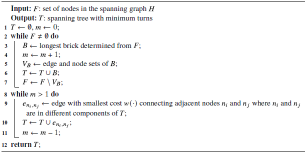
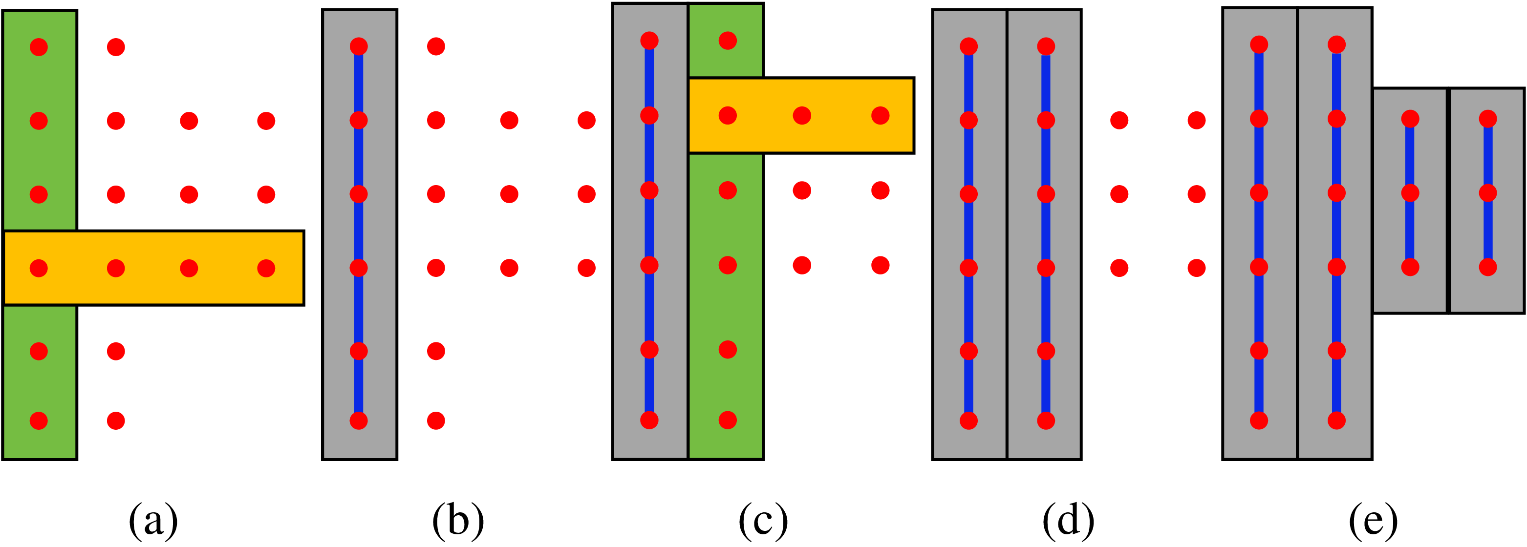
The problem of minimizing the number of bricks is addressed in the TMSTC* algorithm by solving the minimum vertex cover problem on a bipartite graph. In contrast, our method adopts a greedy-based strategy: select the longest brick from the spanning tree node set, remove the nodes contained in the brick from the set, and repeat this process until the set is empty. The greedy process is illustrated in Figure 7, and the corresponding pseudocode can be found in lines 1–7 of Algorithm2.
Figure 7(a) shows the initial state, where all nodes can be used to construct bricks, and the longest vertical and horizontal bricks are selected as candidates. Figure 7(b) illustrates that the longest brick is chosen from the candidate set, and the nodes within this brick are connected as part of the final spanning tree. Figure 7(c) shows that, after removing the connected nodes, the remaining nodes are used to construct new bricks, and the longest vertical and horizontal bricks are again selected as candidates. Figures 7(d)–(e) show that this process is repeated until no remaining nodes can be used to form bricks.
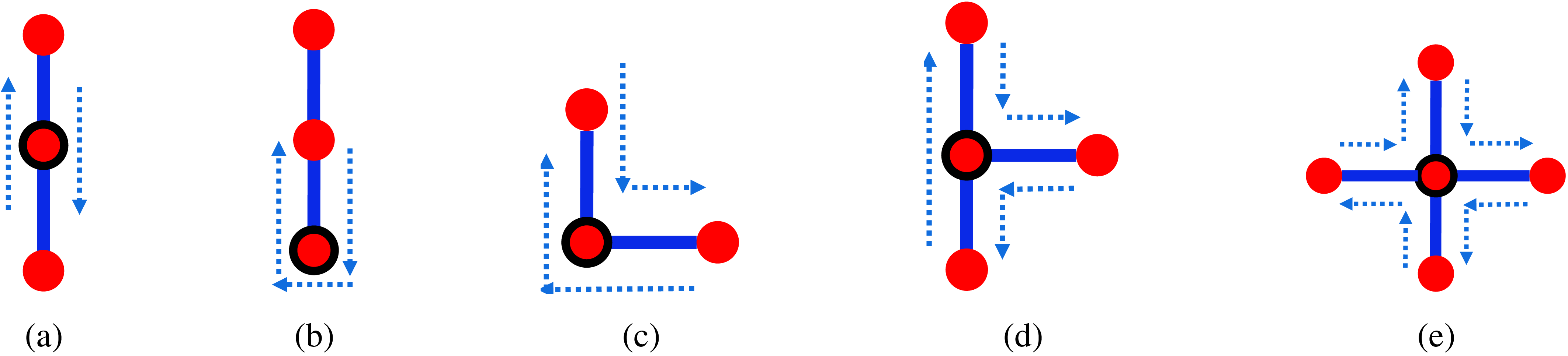
As shown in Table II and Figure 8, spanning tree nodes are classified into five categories, with each category corresponding to a specific number of turns, denoted as
 $f(n)$
. Here,
 $n$
represents a node in the spanning tree
 $H$
, and each node
 $n$
corresponds to a grid cell
 $g$
in the map.
Minimize the number of turns

Algorithm 2 Long description
The pseudocode begins with input F, the set of nodes in the spanning graph H, and output T, the spanning tree with minimum turns. It initializes T as an empty set and m as 0. The while loop continues until F is not empty. Inside the loop, the longest brick is determined from F, and m is incremented by 1. The edge and node sets of the brick are stored in V subscript B. T is updated by taking the union of T and V subscript B, and F is updated by removing the nodes in V subscript B. Another while loop runs while m is greater than 1. Inside this loop, the edge with the smallest cost connecting adjacent nodes in different components of T is found and added to T. m is then decremented by 1. The process repeats until m is 1. Finally, the spanning tree T is returned.
Illustration of the greedy process for selecting the minimal number of bricks. Green and orange represent the longest vertical and horizontal candidate bricks, respectively, while gray indicates the brick
 $B$
selected by the greedy algorithm; blue highlights the spanning tree trunk within
 $B$
.

Therefore, the difference in the number of turns before and after adding a candidate edge to the spanning tree can be calculated:
 \begin{equation} \begin{aligned} w(n_1, n_2) &= f^{+}(n_1) + f^{+}(n_2) - f(n_1) - f(n_2) \end{aligned} \end{equation}
Here,
 $f^{+}(n_1)$
and
 $f^{+}(n_2)$
denote the number of turns at
 $n_1$
and
 $n_2$
after adding the edge
 $e_{n_1,n_2}$
, respectively.
To minimize the number of turns, at each step we select an edge from the candidate edges that connect two adjacent bricks, where both bricks are not yet in the spanning tree
 $ T$
, and choose the edge with the minimum value of the function
 $ W(n_1, n_2)$
. After selecting the edge, it is added to the spanning tree
 $ T$
, connecting the two bricks. This process is repeated
 $ m-1$
times to construct the minimum-turn spanning tree. The corresponding steps are shown in lines 8–11 of Algorithm2.
Number of turns for different node categories.

Table II. Long description
A table comparing the number of turns for different node categories. The table has four columns and one row. Column headers are I, L, + Leaf, and T. Row 1: I, 0; L, 2; + Leaf, 4; T, 2.
Five typical node types in the spanning tree
 $T$
(
 $\mathrm{I}$
-type, leaf,
 $\mathrm{L}$
-type,
 $\mathrm{T}$
-type, and
 $+$
-type) with corresponding turn numbers. The dotted blue arrow indicates the robot’s trajectory.

Comparison of two distance metrics used in DAWG. (a) Manhattan distance, with an average of 316.5 turns. (b) Chebyshev distance, with an average of 213.5 turns.

As shown in Figure 9, we found that during the size division phase, different distance metrics affect the average number of turns of each robot. When wavefront propagation is performed using Manhattan distance and Chebyshev distance, the average number of turns for each robot is 316.5 and 213.5, respectively. Theoretically, when wavefront propagation is carried out using these two different distance metrics, the isochrones of the wavefront are square and diamond-shaped, respectively, which leads to differences in the number of turns at the boundaries of the subareas. Therefore, in the area equal division phase, using Chebyshev distance for wavefront propagation can further reduce the number of turns of each robot.
5. Results & analysis
The experiments were conducted on a device with an Intel Core i5-11,400 processor (2.60 GHz) and 16 GB of memory. Our code is open-source and available on GitHub.
Parameter: In DARP, the maximum number of iterations was set to be nearly infinite. For the other three algorithms, the experimental parameters were kept consistent with the descriptions in the original papers.
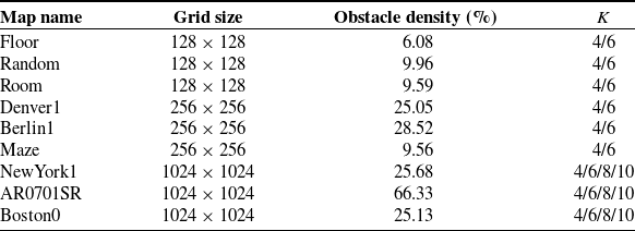
Instances: As shown in Table III, we generated 24 test instances by placing different numbers of robots, denoted as
 $ K$
, on 9 maps with varying obstacle distributions. The values of
 $ K$
are selected with reference to ref. [Reference Tang, Sun and Zhang16]. Each instance corresponds to a specific robot distribution on a given map. Among these, the first map is a typical floor map created by the authors, while the remaining eight maps are sourced from the widely used 2D pathfinding benchmarks [Reference Sturtevant28]. The existing large-scale MCPP study [Reference Tang and Ma24] is conducted on a map of size
 $256 \times 256$
. Therefore, in our experiments, we define maps of size
 $256 \times 256$
and above as large-scale maps, while other maps are referred to as small-scale maps.
Furthermore, to provide a more comprehensive evaluation of the proposed method, the test maps are designed by considering three key factors: map scale, obstacle density, and the distribution of initial robot positions. As shown in Figure 14(c), on the map *Room*, the obstacle density is only 9.59%, and the initial positions of the four robots (indicated by white pentagrams) are highly clustered. In contrast, as shown in Figure 14(d), the map *AR0701SR* has a high obstacle density of 66.33%, and the initial positions of the 10 robots are more spatially dispersed.
MCPP instance specifications.

Table III. Long description
The table compares map names, grid sizes, obstacle densities, and K values for different instances. It has four columns: Map name, Grid size, Obstacle density (percent), and K. The table includes nine rows with the following data: Row 1: Floor, 128 x 128, 6.08, 4/6. Row 2: Random, 128 x 128, 9.96, 4/6. Row 3: Room, 128 x 128, 9.59, 4/6. Row 4: Denver1, 256 x 256, 25.05, 4/6. Row 5: Berlin1, 256 x 256, 28.52, 4/6. Row 6: Maze, 256 x 256, 9.56, 4/6. Row 7: NewYork1, 1024 x 1024, 25.68, 4/6/8/10. Row 8: AR0701SR, 1024 x 1024, 66.33, 4/6/8/10. Row 9: Boston0, 1024 x 1024, 25.13, 4/6/8/10.
5.1. Solvability comparisons
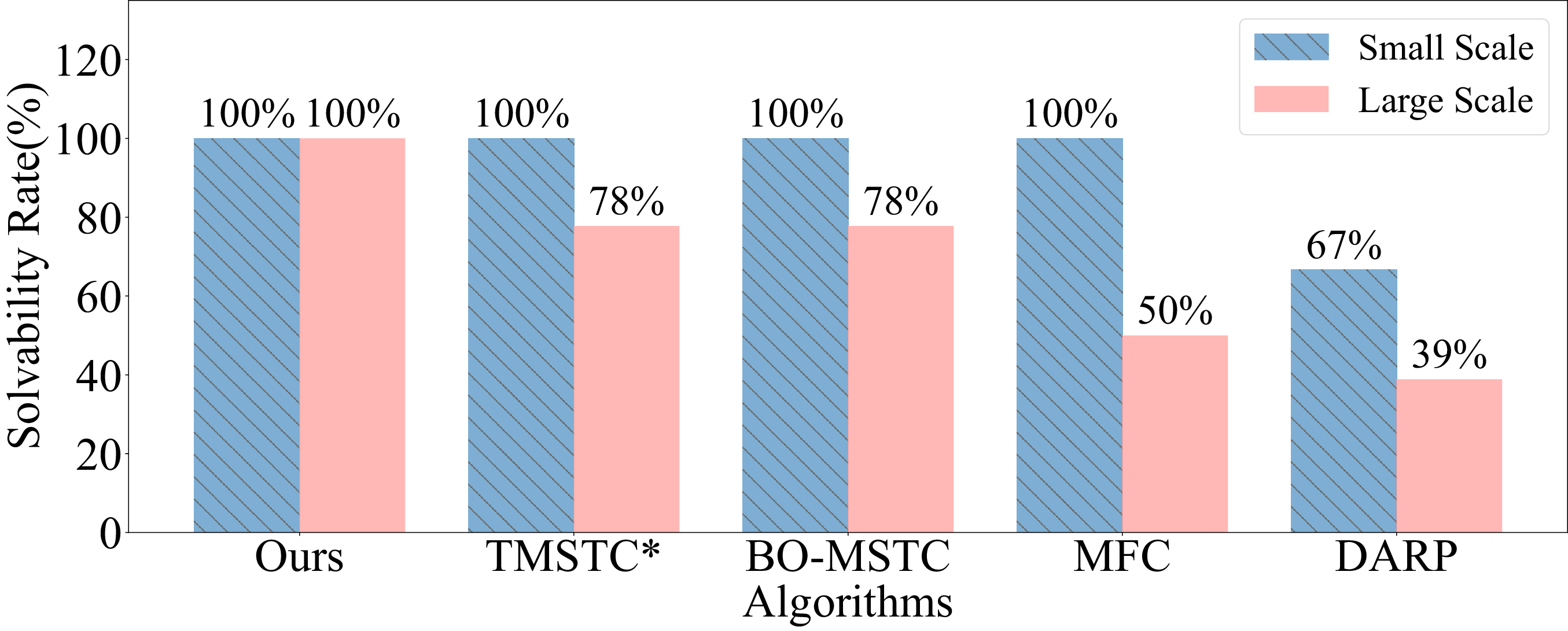
In this letter, the solvability of an algorithm is defined as whether it can produce the result of coverage path planning within 3 hours. To evaluate the solvability of our algorithm compared to other existing algorithms, we conducted experiments on both small-scale and large-scale maps.
As shown in Figure 10, our algorithm achieves 100% solvability on both small-scale and large-scale maps, while DARP fails on some maps. Furthermore, although BO-MSTC, MFC, and TMSTC* are not MCPP algorithms based on size division, their solvability rate on large-scale maps is still below 100%. These results demonstrate that the proposed DAWG algorithm exhibits stronger solvability in large-scale maps.
Comparison of solvability rates on large-scale and small-scale maps using DAWG and baseline algorithms.

5.2. Path length and number of turns comparison
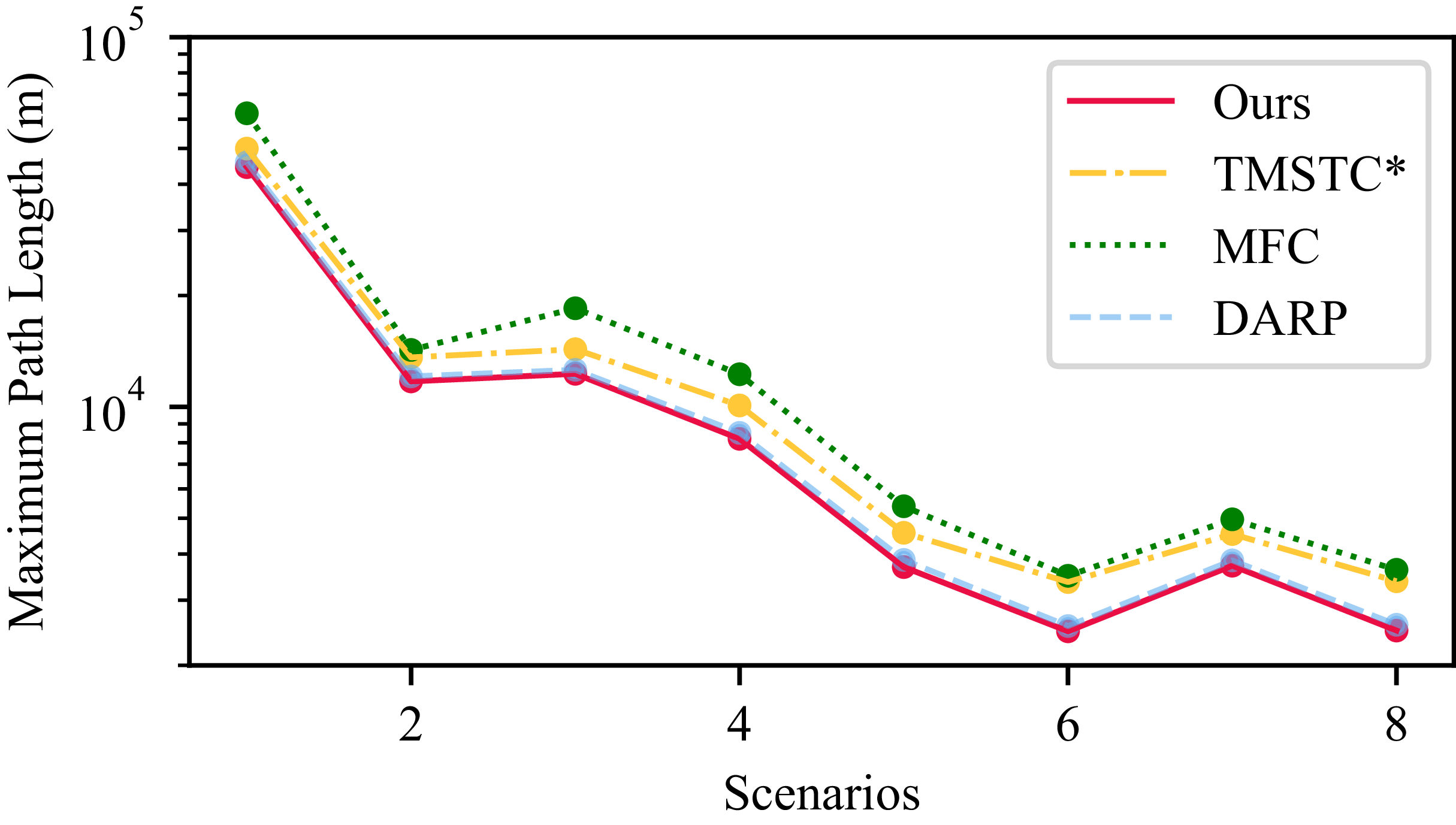
To compare the maximum coverage path lengths between our proposed algorithm and existing methods, we selected the intersection of solvable instances across four algorithms: DAWG, DARP, TMSTC*, and MFC. Figure 11 presents the maximum coverage path length among the
 $K$
robots for each of the eight instances (the specific values of
 $K$
are provided in Table III). Based on these results, we can observe that both our DAWG algorithm and the DARP algorithm, as size division-based MCPP approaches, achieve comparable and relatively shorter maximum coverage path lengths than the other two methods that do not employ size division.
Comparison of maximum coverage path length among four algorithms.

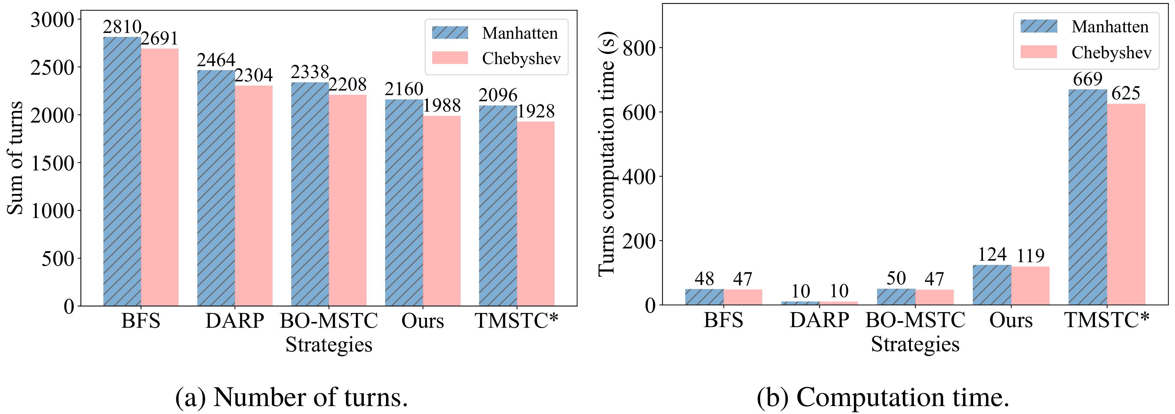
To evaluate the performance of our Chebyshev distance-based size division and Greedy–Kruskal spanning tree construction strategy in reducing turns, we calculated the average total number of turns and the computation time for the spanning tree construction process. Four existing strategies were compared: DARP (using DFS), TMSTC*, BO-MSTC (using Kruskal), and BFS. Figure 12(a) shows the total average turns for size division using Manhattan and Chebyshev distances under different spanning tree construction strategies. The use of Chebyshev distance consistently resulted in fewer turns compared to Manhattan distance, indicating that it optimizes subarea shapes and reduces turns within each spanning tree. Notably, as shown in Figure 12, our method incurs only 3% more turns than TMSTC*, while the computation time is reduced by 81%.
Comparison of the number of turns and computation time required to construct the spanning tree.

5.3. Coverage time comparisons
To ensure a fair comparison, we adopt the same coverage time calculation method as described in TMSTC*. Specifically, the time
 $ t_j$
required for a robot to move between two consecutive turning points
 $ \gamma _j$
and
 $ \gamma _{j+1}$
in the path
 $ \Pi _i$
is computed as follows, where a turning point is defined as a point where the robot’s direction of motion changes:
 \begin{equation} t_j = \begin{cases} \sqrt {\dfrac {d_{\gamma _j,\gamma _{j+1}}}{a}}, & \text{if } d_{\gamma _j,\gamma _{j+1}} \leq \dfrac {v_{\max }^2}{a}, \\[12pt] \dfrac {d_{\gamma _j,\gamma _{j+1}}}{v_{\max }} + \dfrac {v_{\max }}{a}, & \text{otherwise}. \end{cases} \end{equation}
Here,
 $ d_{\gamma _j,\gamma _{j+1}}$
denotes the Euclidean distance between two turning points,
 $ v_{\max }$
is the maximum velocity, and
 $ a$
is the constant acceleration. The time spent on turning is also considered, where each turn costs
 $ \frac {\pi }{2\omega }$
, and
 $ \omega$
represents the constant angular velocity. Other kinematic parameters and implementation details are consistent with those provided in ref. [Reference Lu, Zeng, Tang, Lam and Wen17]. Additionally, in our experiments, we assume that robots can only move in four directions (up, down, left, right). Therefore, we made corrections to the coverage paths obtained from the TMSTC*, BO-MSTC, and MFC algorithms, where it is assumed that robots can move in eight directions. Specifically, when diagonal movement occurs in the path, we decompose it into two components along the horizontal and vertical directions using vector decomposition.
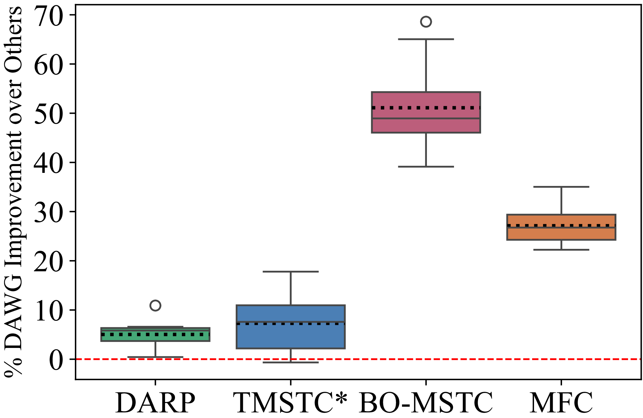
Box plot of the performance improvement percentages of the proposed DAWG algorithm compared with four other algorithms, with dashed lines representing the mean. The mean performance improvement ratios relative to DARP, TMSTC*, BO-MSTC, and MFC are
 $5\%$
,
 $7.3\%$
,
 $51.1\%$
, and
 $27.1\%$
, respectively.

In the MCPP problem, coverage time is defined as the time taken for the last robot to complete its coverage task. As shown in Figure 13, to evaluate the effectiveness of the proposed algorithm in comparison with existing algorithms, we calculated the coverage time improvement percentage of DAWG relative to DARP, TMSTC*, BO-MSTC, and MFC. The results indicate that DAWG achieves an average coverage time improvement of 5%, 7.3%, 51.1%, and 27.1%, respectively, over the aforementioned four baseline algorithms across all test cases (assuming the algorithm is solvable for each test case). The experimental results clearly demonstrate that our algorithm outperforms all baseline algorithms in terms of coverage time, establishing it as an effective solution to the MCPP problem in large-scale maps.
Figure 14 illustrates the coverage path planning results of DAWG applied to four test cases of varying scales. In Figure 14(c) and (d), due to the larger map scale, the paths are more densely packed. In the maps, white pentagrams represent the initial positions of the robots, black regions indicate obstacles, and the coverage paths of different robots are distinguished using different colors.
Four different environments and the corresponding coverage path planning results using the proposed DAWG algorithm: (a) Room,
 $128\times 128$
, with 4 robots; (b) Maze,
 $256\times 256$
, with 6 robots; (c) Boston0,
 $1024\times 1024$
, with 8 robots; and (d) AR0701 SR,
 $1024\times 1024$
, with 10 robots.

5.4. Computation time comparisons
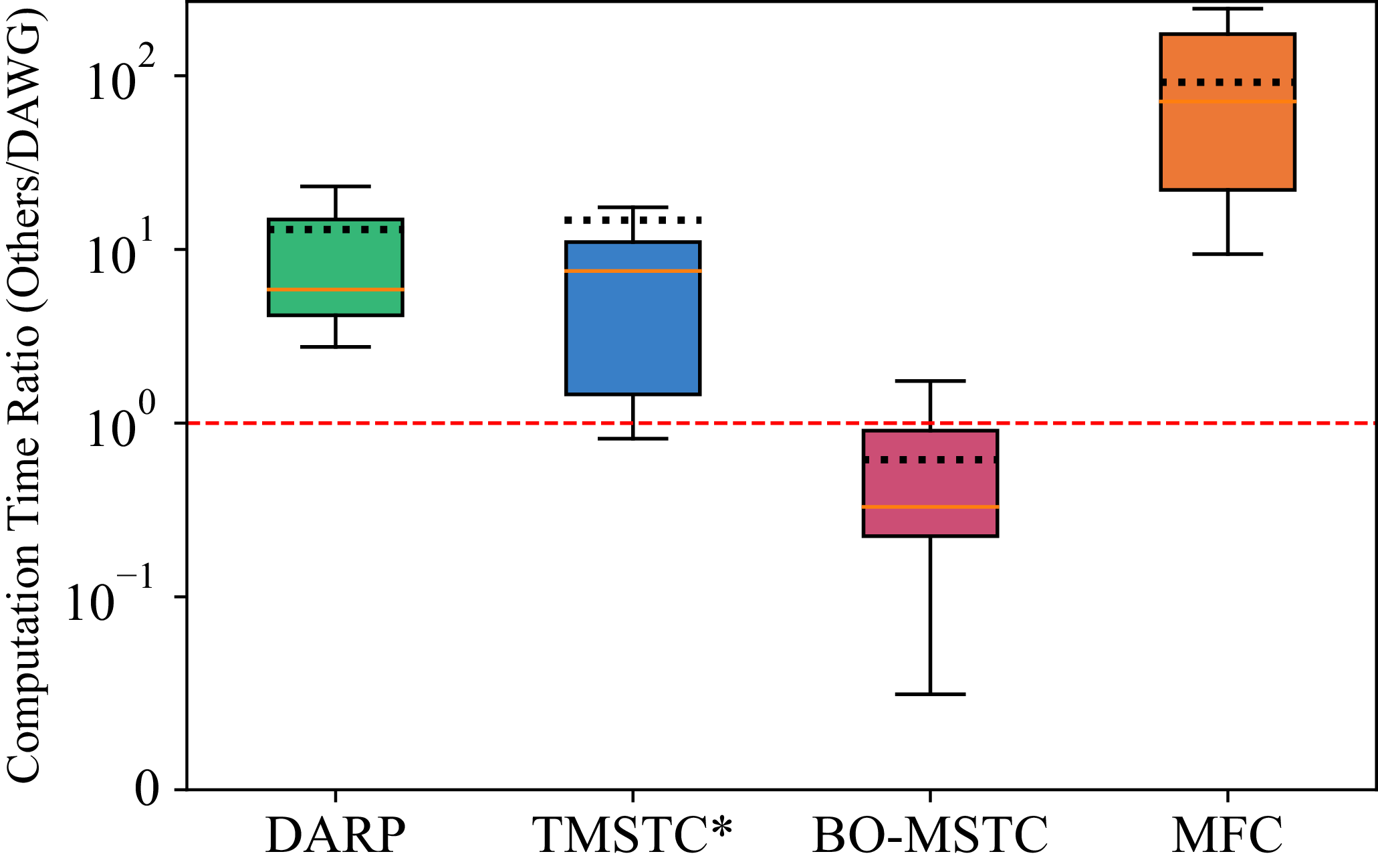
We computed the ratio of the computation time of DAWG relative to the four existing algorithms across all test cases (assuming the algorithm is solvable for each test case). As shown in Figure 15, the average ratios of the computation time of DAWG to DARP, TMSTC*, BO-MSTC, and MFC are 13, 14.7, 0.6, and 91.6, respectively. It can be seen that, compared to the other four algorithms, our proposed DAWG algorithm has a computation time only slightly longer than BO-MSTC. Compared to BO-MSTC, DAWG reduces coverage time by 51.1% and increases solvability by 33% on large-scale maps. More importantly, DAWG algorithm, compared to the existing SOTA algorithms, not only has shorter coverage time but also lower computational cost.
Box plot showing the ratio of the computation time of DARP, TMSTC*, BO-MSTC, and MFC to that of DAWG, with the mean indicated by the dashed line. The mean ratios are 13, 14.7, 0.6, and 91.6, respectively.

6. Conclusions
In this letter, the proposed DAWG algorithm achieves path length minimization by equally dividing free area. To address the issue of TMSTC*’s long computation time on large-scale maps, a greedy strategy is introduced, which significantly reduces computation time compared to TMSTC* while ensuring near-optimal turn counts. The overall coverage time of this algorithm is shorter than that of SOTA algorithms, while its computation time remains at a low level. Additionally, experimental results demonstrate that DAWG exhibits higher solvability on large-scale maps.
The proposed method has potential applications in various real-world scenarios, such as cleaning and inspection tasks in large indoor environments. However, it still has certain limitations. Since the method is based on spanning tree construction, it imposes specific requirements on map modeling, that is, the grid size must match the robot size. In practice, the grid size may be smaller than the robot size. This makes it difficult for the robot to enter narrow areas and reduces the overall coverage rate. To balance coverage and efficiency, future work may consider size-adaptive robots as proposed in refs. [Reference Samarakoon, Muthugala and Kalimuthu25, Reference Samarakoon, Muthugala, Kalimuthu, Chandrasekaran and Elara26]. Such robots can maintain a larger size in open areas to improve coverage efficiency. They can also reduce their size in narrow areas to enhance accessibility. It should be noted that, when the speed remains constant, reducing the robot size decreases the area covered per unit time, which lowers coverage efficiency. By using size adaptation, a high coverage rate can be maintained while mitigating its negative impact on coverage efficiency.
Author contributions
Yiyi Zhang and Renjie Guo contributed equally to this work; Yiyi Zhang and Renjie Guo conceived and designed the study, and conducted the experiments; Peng Guo supervised the project and provided critical revisions to the manuscript. All authors read and approved the final manuscript.
Financial support
This research was supported by the National Key Research and Development Program of China under Grant 2024YFC3811102.
Competing interests
The authors declare no conflicts of interest exist.
Ethical approval
Not applicable.
 512×512

 G
 H



 B
 B

 T
 I
 L
 T
 +

 5%
 7.3%
 51.1%
 27.1%

 128×128
 256×256
 1024×1024
 1024×1024