1. Introduction
Turbulence remains one of the most challenging unresolved problems in classical physics, appearing across a wide range of spatial and temporal scales in both natural environments and engineered systems. In aerospace engineering, turbulent flows have a direct impact on aerodynamic performance, and accurate turbulence prediction is essential for the efficient design, optimisation and safe operation of aircraft. Owing to the high cost and limited repeatability of experimental approaches, as well as their inability to provide sufficient details for researchers to gain a comprehensive understanding of the flow phenomenon, computational fluid dynamics (CFD) has become an indispensable tool for simulating and understanding turbulent flows in modern aerospace design processes (Sandberg & Michelassi Reference Sandberg and Michelassi2022).
High-fidelity simulation methods, such as direct numerical simulation (DNS) and large-eddy simulation (LES), remain impractical for complex geometries due to their prohibitive computational cost. As a result, the Reynolds-averaged Navier–Stokes (RANS) approach continues to be the primary tool for industrial design for decades to come owing to its cost effectiveness and robustness. However, the predictive accuracy of RANS is limited by model uncertainties. Both the inherent assumptions in RANS-based turbulence modelling and the process of formulating model closures introduce potential model uncertainty, including the information loss in the Reynolds-averaging process, uncertainties in the Reynolds stress constitutive relations and structural as well as parametric uncertainties in the turbulence transport equations (Xiao & Cinnella Reference Xiao and Cinnella2019; Duraisamy, Iaccarino & Xiao Reference Duraisamy, Iaccarino and Xiao2019). Suffering from these significant model uncertainties, RANS models manifest obvious applicability defects in predictive capability when applied to complex flow scenarios involving separation, transition and strong shear. Enhancing the performance of RANS in such challenging flow regimes has become one of the central issues in the development of CFD.
In recent years, driven by the continuous growth of computational resources, the rapid advancements in relevant efficient algorithms and the increasing availability of high-fidelity data, the application of artificial intelligence techniques to fluid dynamics has experienced significant development (Brunton, Noack & Koumoutsakos Reference Brunton, Noack and Koumoutsakos2020; Zou et al. Reference Zou, Xu, Chen, Yao and Fu2024). Owing to the limited predictive accuracy of traditional turbulence models in capturing complex flow structures, data-driven turbulence modelling has attracted widespread attention. These approaches leverage statistical learning or machine learning (ML) techniques to incorporate information from experiments or high-fidelity numerical simulations, with the aim of correcting or reconstructing existing models to enhance both their accuracy and generalisation capability. Based on how the corrections are incorporated into the RANS equations, current mainstream data-driven approaches can be broadly classified into two categories: those that directly modify the Reynolds stress or eddy viscosity, and those that instead embed the corrections into the turbulence transport equations. In studies aiming to directly establish the mapping from mean flow features to Reynolds stresses using ML techniques, Wang, Wu & Xiao (Reference Wang, Wu and Xiao2017) proposed a data-driven framework in which the discrepancy between Reynolds stresses predicted by RANS and those obtained from DNS was used as the learning target. By employing random forest algorithms, they developed Reynolds stress discrepancy models conditioned on multiple local flow features, enabling the reconstruction of Reynolds stress to improve RANS predictions. Since the prediction is performed independently at each grid point, the resulting Reynolds stress field may exhibit spatial non-smoothness. Moreover, the accurate prediction of Reynolds stress does not inherently translate to improved mean-flow predictions. To alleviate the ill-conditioning issues associated with the explicit correction of Reynolds stress, Wu, Xiao & Paterson (Reference Wu, Xiao and Paterson2018) predicted the nonlinear components of Reynolds stress and the optimal eddy viscosity separately. This implicit treatment enhances the prediction of mean-flow quantities. However, directly predicting the Reynolds stress tensor may violate its inherent symmetry, potentially leading to physically inconsistent results. He et al. (Reference He, Tan, Rigas and Vahdati2022a ) further simplified the problem by modelling scalar eddy-viscosity discrepancies, allowing reduced data requirements. Their results demonstrated that correcting eddy viscosity can improve the baseline model’s predictive accuracy in transonic flows. Furthermore, post hoc analyses were conducted to investigate the distribution of input features across different flow regions and their influence on the predicted eddy-viscosity discrepancies, providing interpretable visualisations that help associate high-error regions with specific flow phenomena. Other studies focusing on the correction of eddy viscosity have also demonstrated improved predictive performance of the existing turbulence model in challenging scenarios such as compressor transonic or near-stall flows (Lee, Wilson & Vahdati Reference Lee, Wilson and Vahdati2018; Moreno et al. Reference Moreno, Dodds, Stapelfeldt and Vahdati2020; He et al. Reference He, Zhao and Vahdati2022b ; Wu et al. Reference Wu, Wang, Zhang and He2023), highlighting this approach as an effective strategy for enhancing the accuracy of RANS simulations. To improve the physical interpretability of corrections trained for traditional RANS models, Weatheritt & Sandberg (Reference Weatheritt and Sandberg2016) employed gene-expression programming to derive explicit algebraic stress models for the nonlinear part of the Reynolds stress anisotropy. Their method yielded consistent improvements in several a posteriori tests for similar types of flows. Building on this direction, Schmelzer, Dwight & Cinnella (Reference Schmelzer, Dwight and Cinnella2020) and Cherroud et al. (Reference Cherroud, Merle, Cinnella and Gloerfelt2022) respectively developed the deterministic symbolic regression method SpaRTA (sparse regression of turbulent stress anisotropy) and introduced a sparse Bayesian learning framework to identify interpretable additional terms for the anisotropic part of the Reynolds stress as well as for the transport models. These studies demonstrated that a correction only for the source terms in the transport models could sufficiently improve the predictive accuracy for two-dimensional separated flows, even without directly modifying the constitutive relation. Furthermore, the use of sparse regression techniques not only reduced computational cost but also facilitated the discovery of compact models with high accuracy for specific classes of flows.
The research efforts that associate corrections with the transport equations are primarily based on the field inversion and machine learning (FIML) framework proposed by Parish & Duraisamy (Reference Parish and Duraisamy2016). This approach leverages high-fidelity (Hi-Fi) data, obtained from numerical simulations and experiments, to infer the spatial distribution of correction term for minimising the deviation between the RANS simulation result and Hi-Fi solution. Subsequently, ML techniques are employed to construct models that relate flow-dependent features to the inferred corrections. Based on the FIML framework, Singh, Medida & Duraisamy (Reference Singh, Medida and Duraisamy2017) and Ferrero, Iollo & Larocca (Reference Ferrero, Iollo and Larocca2020) applied adjoint-based methods to obtain spatially varying correction fields introduced into the turbulence models. These corrections were then used to train ML models in the context of separated flows over airfoils and turbomachinery, respectively. When applied to test cases beyond the training set, the learned models demonstrated satisfactory predictive accuracy, indicating that the proposed correction strategy for the transport equations is effective in capturing separation phenomena. However, adjoint-based methods are often limited by their computational complexity, and the resulting ML models are often black box in nature, lacking interpretability and physical insight. To address these limitations, Zhang et al. (Reference Zhang, Xiao, Luo and He2022, Reference Zhang, Xiao, Jee and He2023) proposed an iterative Ensemble Kalman Filter (EnKF) method to learn the weights of a neural network, which learns the relationship between scalar invariants and the scalar coefficient functions. The deviatoric part of the Reynolds stress is then constructed from the neural-network outputs and tensor bases (Pope Reference Pope1975). The use of ensemble-based methods enables the learning of underlying Reynolds stress closures from sparse Hi-Fi data, thereby improving the predictive accuracy of traditional turbulence models for flow separation. Moreover, the model-consistent learning framework embedding the neural-network-based turbulence model in the RANS equations helps alleviate the ill conditioning of the trained model and the discrepancies between training and prediction (Wu et al. Reference Wu, Xiao, Sun and Wang2019).
Considering the advantages and limitations of existing approaches, this work proposes an ensemble-based data assimilation framework for deriving a simple and physically expressive closed-form correction expression embedded in the transport equations of turbulence models. Distinct from many prior studies that infer high-dimensional neural-network weights for model correction, the present work represents the correction field using a linear combination of one-dimensional Gaussian functions with only a few physically interpretable parameters. By decomposing the correction into feature-specific components, this compact formulation reduces the dimensionality of the inference problem and provides a structured means to associate distinct flow features with corresponding correction directions. By incorporating prior physical knowledge that model corrections are required only in localised regions of the flow field (Ling & Templeton Reference Ling and Templeton2015; Jäckel Reference Jäckel2021) and utilising the ensemble method (Evensen Reference Evensen2003), the correction expression is embedded into the RANS solver and activated in a finite region selectively. Furthermore, the use of flow-relevant input features for both training the correction expression and clustering the correction-activated regions enables a closer connection between the inferred correction and the governing flow dynamics, thereby improving its adaptability and generalisation across flows with similar physical characteristics. This perspective is also supported by recent studies that emphasise the role of structurally constrained and explicitly expressed correction models in achieving robust generalisation. The LIFE (learning and inference assisted by feature-space engineering) framework (Srivastava & Duraisamy Reference Srivastava and Duraisamy2021) employs piecewise-linear representations together with integrated inference and learning to explicitly constrain the feature-to-correction mapping across datasets. While sharing a similar motivation of constraining model expressiveness, the present approach adopts a compact closed-form correction embedded directly into the transport equations, leading to different trade-offs in interpretability, implementation complexity and inference strategy. The coefficients of the correction expression are optimised based on the discrepancy between sparse Hi-Fi data and RANS predictions, yielding a concise correction term that effectively reduces the computational error of the baseline model. This framework provides several key advantages, including reduced training costs, more effective utilisation of limited Hi-Fi data through observation augmentation and improved model generalisation. Moreover, it provides a novel perspective for constructing high-accuracy turbulence models that are compatible with solver implementation. Specifically, the proposed framework offers three main benefits. First, the correction expression is physics informed and compact, enabling convenient integration into existing solvers. The reduced complexity facilitates the identification of shared flow features, thereby enhancing the model’s generalisation capability across diverse flow conditions. Second, integrating the correction model with CFD calculations during training enables it to automatically adapt to flow pattern variations by taking the feedback of the flow field into account. This approach maintains consistency between training and prediction and reduces the computational burden associated with post-training manual adjustments and validation. Moreover, by introducing implicit physical constraints, it reduces reliance on purely data-driven fitting and enhances the robustness of corrections across different applications. Finally, inferring coefficients of correction expression via ensemble-based method significantly reduces the dimensionality of the state vector compared with learning the spatial distribution of the correction term directly. Furthermore, the multi-fidelity data aggregation model based on convolutional neural networks (CNN) effectively leverages limited Hi-Fi observations, resulting in more accurate RANS predictions with improved capability to capture the underlying flow physics.
The rest of this paper is organised as follows. Section 2 details the proposed turbulence modelling framework, which applies a model-consistent correction based on radial basis functions (RBF). The case set-up, training and testing results are presented and analysed in § 3, and the influence of the selection of observation data on the training process and model output is also evaluated. Finally, the conclusions obtained in this paper are summarised in the § 4.
2. Radial-basis-function-based corrections and data assimilation with fused multi-fidelity observations
This section presents the specific methodologies employed in this study. First, the baseline Spalart–Allmaras (S–A) turbulence model is introduced, along with the formulation of the correction term expressed using RBF. Subsequently, an ensemble-based data assimilation method is described, which integrates the FIML-Direct approach proposed by Holland et al. (Reference Holland, Baeder and Duraisamy2019a ,Reference Holland, Baeder and Duraisamy b ) with CFD calculations. This integration enables the derivation of correction expressions that account for the influence of iterative correction. Finally, the selection of observation data and the model training strategies adopted within the ensemble-based method are briefly described.
2.1. Corrections based on a radial-basis-function form
In this study, the one-equation S–A turbulence model (Spalart & Allmaras Reference Spalart and Allmaras1992) is adopted as the baseline for introducing corrections. This choice is motivated by the model’s simple structure, high computational efficiency and widespread application in engineering flows, particularly in aerospace problems, making it both practical and representative for data-driven turbulence model development. The transport equation of the S–A model reads
 \begin{equation} \frac {\partial \tilde {\nu }}{\partial t}+{{u}_{\!j}}\frac {\partial \tilde {\nu }}{\partial {{x}_{\!j}}}={{C}_{b1}}\tilde {S}\tilde {\nu }-{{C}_{w1}}{{f}_{w}}{{\left ( \frac {{\tilde {\nu }}}{d} \right )}^{2}} +\frac {1}{\sigma }\left ( \frac {\partial }{\partial {{x}_{\!j}}}\left ( \left ( \nu +\tilde {\nu } \right )\frac {\partial \tilde {\nu }}{\partial {{x}_{\!j}}} \right )+{{c}_{b2}}\frac {\partial \tilde {\nu }}{\partial {{x}_{i}}}\frac {\partial \tilde {\nu }}{\partial {{x}_{i}}} \right )\! .\end{equation}
where
 $\tilde{\nu}$
is the working variable of the turbulence model,
 $\nu$
is the kinematic molecular viscosity,
 $u_j$
is a velocity component in the
 $j$
th direction,
 $\tilde{S}$
is the modified strain rate,
 $d$
is the wall distance,
 $\sigma$
is a model constant, and
 $C_*$
and
 $f_*$
denote model coefficients and functions, respectively. The right-hand side of (2.1) comprises production, destruction and transport terms, denoted by
 $\textrm{P}$
,
 $\textrm{D}$
, and
 $\textrm{T}$
, respectively. These terms are simplified as follows (Moreno et al. Reference Moreno, Dodds, Stapelfeldt and Vahdati2020):
 \begin{equation} \frac {{D\tilde \nu }}{{Dt}} = \underbrace {P\left ( {\tilde \nu ,U} \right ) - D\left ( {\tilde \nu ,U} \right )}_{\textit{Source}{\textrm { }}\textit{term}} + \underbrace {T\left ( {\tilde \nu ,U} \right )}_{\textit{Diffusion}} .\end{equation}
The eddy viscosity in the S–A model is estimated by
 \begin{equation} {\nu _t} = {f_{v1}}\tilde \nu \quad {\textrm {where }} \quad {f_{v1}} = \frac {{{\chi ^3}}}{{{\chi ^3} + c_{v1}^3}} \textrm{ and the intermediate variable}\,\chi = \frac {{\tilde \nu }}{\nu }, \end{equation}
For a detailed description of the values of the constants and the terms, the reader is referred to the original publication of the S–A turbulence model (Spalart & Allmaras Reference Spalart and Allmaras1992). The conventional S–A model can provide satisfactory predictions in the attached flow, but it tends to overpredict the eddy viscosity in the presence of an adverse pressure gradient. To reduce the inaccuracies observed in predicting flows with strong non-equilibrium separation characteristics, and motivated by both the model-form deficiencies inherent in the original formulation structure (Singh et al. Reference Singh, Medida and Duraisamy2017) and the improvements made in models such as rotation and/or streamline curvature to account for rotation and curvature effects (Shur et al. Reference Shur, Strelets, Travin and Spalart2000), the following modification is applied to (2.2):
 \begin{equation} \frac {{D\tilde \nu }}{{Dt}} = \beta\kern-1pt P\left ( {\tilde \nu ,U} \right ) - D\left ( {\tilde \nu ,U} \right ) + T\left ( {\tilde \nu ,U} \right ) .\end{equation}
where
 $\beta$
is a spatially varying correction factor. Following the identification of dominant physical processes in different flow domains within the equation space by Callaham et al. (Reference Callaham, Koch, Brunton, Kutz and Brunton2021) using unsupervised learning, and the implementation of region-limiting strategies for augmentation as proposed by Srivastava et al. (Reference Srivastava, Rumsey, Coleman and Wang2024), this study adopts the adaptive selection of regions for correction introduced by Gou, Ye & Zou (Reference Gou, Ye and Zou2025), which confines the specific region for correction through Gaussian mixture models (GMMs). The spatial distribution of the correction term is inferred from Hi-Fi data using the ensemble-based data assimilation method. Meanwhile, this study is based on the FIML-Direct framework (Holland et al. Reference Holland, Baeder and Duraisamy2019a
,Reference Holland, Baeder and Duraisamy
b
), in which FIML are performed in a coupled manner, as opposed to the conventional FIML-Classic framework (Singh Reference Singh2018), where the two processes are carried out separately.
For the first-generation FIML framework, FIML-Classic (Singh Reference Singh2018), which takes a two-step approach, the distribution of
 $\beta$
is first obtained through data assimilation. An ML model is then trained to reproduce this inferred correction as a function of selected mean-flow features. In its typical form, the training uses features extracted from the inverted or converged corrected solution, and during deployment the trained ML model is embedded in the RANS solver so that the correction is re-evaluated and updated at each iteration until convergence. Subsequent studies have also examined a one-time-correction variant of the FIML-Classic framework (Ho & West Reference Ho and West2021) to mitigate the strong dependence of the iterative correction on the initial flow field, thereby reducing the risk of divergence while maintaining comparable accuracy. In this variant, both the training and testing phases use mean-flow features computed from the uncorrected baseline solution. During testing, the predicted correction is obtained from the baseline features and then embedded in the RANS solver as a fixed source term while the equations are iterated to convergence, ensuring that the correction is assessed under conditions consistent with those in training.
Motivated by the same considerations of reducing the sensitivity to the initial flow field and ensuring consistency between the training and testing environments, we refer to ‘FIML-Classic’ as the one-time-correction variant in the present study. Taken together, the training and testing procedures of the full FIML-Classic workflow involve four separate applications of the RANS solver, corresponding to the key stages outlined in figure 1.
Schematic of the FIML-Classic framework with the one-time-correction approach, including the standalone ML model construction and the four stages involving RANS solver usage in both training and testing. The predicted correction is frozen and embedded into the RANS solver for the final augmented computation. Here,
 $q_i$
denotes the
 $i$
-th input feature.

The FIML-Direct framework integrates FIML into a unified process by directly inferring the weights of the neural network whose output represents the correction term. In this framework, the correction distribution is learned during the inversion, eliminating the need for a separate ML stage as in FIML-Classic. Considering that RBF can be interpreted as a simplified form of neural networks, an alternative strategy is to represent the correction distribution using an RBF-based simple algebraic expression calculated based on the flow features, which is structurally analogous to the neural-network model employed in the ML stage of FIML-Classic. In this spirit, Jäckel (Reference Jäckel2023) demonstrated that explicitly structured, closed-form correction expressions based on localised basis-function formulations can effectively act as separation corrections and lead to tangible improvements in separated-flow predictions. Compared with the less interpretable black-box models, the simple RBF-based formulation adopted in this work reduces model complexity and imposes less stringent requirements on the accuracy of fitting the correction distribution, which is usually required in FIML-Classic. This also increases the potential for better generalisation across different flow cases. Notably, representing the correction distribution using explicit expression avoids the necessity of training a shared ML model on data from multiple cases. Especially when there are non-unique mappings and redundant or noisy samples in the training data, it is relatively difficult to establish a ML model with higher accuracy. A similar motivation underlies the LIFE framework (Srivastava & Duraisamy Reference Srivastava and Duraisamy2021), which does not aim to optimally determine the range of influence of the learned correction, but instead emphasises the necessity of localised learning to improve generalisability and to mitigate spurious behaviour arising from extrapolation within a bounded feature space. The overall procedure of FIML-Direct is illustrated in figure 2. In contrast to FIML-Classic, which requires a dedicated ML model construction process, FIML-Direct also simplifies the workflow by requiring the RANS solver use only for the calculation with the correction model in the training and testing phases. With the correction expression embedded directly into the solver, it bypasses the need for separate input features collection.
Schematic of the FIML-Direct framework, implementing the correction through parameter inference of a predefined functional form and eliminating the need for a separate ML model construction and input features collection. The RBF-based correction structure is embedded into the RANS solver prior to data assimilation, then the assimilation process estimates the optimal parameters by matching high- and low-fidelity (Lo-Fi) data. The identified functional correction is then directly embedded into the RANS solver for augmented simulations. Here,
 $\eta$
denotes the input feature, and
 $a,\,b,\,\text{and}\,c$
denote the coefficients of the predefined functional form.

In previous studies, the inferred correction values were found to be both greater than and less than the original term in different spatial regions, indicating that the correction is not limited to reducing the eddy viscosity of the baseline model. In some areas, an increased eddy viscosity may be needed. To accommodate this, the RBF-based correction expression used in this work is designed to correspond to the number of selected input features. The assimilation targets in the FIML-Direct approach therefore include the RBF centres and widths for each feature, as well as the weights used in the linear combination of these features. The formulation is summarised as follows:
 \begin{equation} \beta \left ( {{\eta _1},{\eta _2} \ldots } \right ) = 1 - \sum \limits _{i = 1}^n {{a_i}} {e^{ - \tfrac {{{{\left ( {{\eta _i} - {b_i}} \right )}^2}}}{{2{c_i}^2}}}} .\end{equation}
This reflects that, in the multi-dimensional feature space, the proposed correction employs a weighted superposition of one-dimensional RBFs, combined with the baseline
 $\beta$
value of 1. Here, n in (2.5) denotes the number of such one-dimensional RBF terms, each associated with one selected input feature. The value of n can be adjusted according to the specific problem. This construction leads to a feature-wise RBF-inspired representation that retains the locality, smoothness and nonlinear mapping characteristics. Such a representation provides a compact and interpretable correction model that is well suited to the current data assimilation setting. Therefore, denoting the proposed correction as an RBF-based formulation not only emphasises its structural characteristics but also, considering the extensive use of RBFs in neural networks and support vector machines, suggests that this correction can act as a simple neural-network surrogate within the FIML framework.
By employing this correction expression to improve the prediction accuracy of the S–A model for separated flows, the computational cost of field inversion becomes independent of the computational domain of specific flow cases. Instead, it scales proportionally with the number of selected input flow features. The correction expression depends independently on each input feature, with each feature represented by its own one-dimensional Gaussian RBF, rather than using a vector-form RBF that couples multiple features. This design balances the simplicity of the expression, physical interpretability and computational effectiveness. Specifically, using n one-dimensional Gaussian RBFs allows clear understanding of each feature’s contribution to the model correction: parameter
 $a_i$
controls the magnitude of the correction, reflecting the contribution of the corresponding feature; parameter
 $b_i$
sets the activation threshold, producing significant correction only when the feature value is near this threshold; and parameter
 $c_i$
determines the spatial extent of the correction. The local non-zero property ensures that the correction approaches the baseline RANS value far from the active regions. In addition, analyses of simulation results show that using a vector-form correction with the same number of features and parameter perturbations leads to narrower distributions and less agreement with Hi-Fi data, whereas the proposed expression demonstrates sufficient expressiveness and flexibility. Moreover, treating the contributions of different physical features independently facilitates model interpretability and provides a foundation for future incorporation of additional features that can guide the correction.
In this study, the CFD simulations are carried out using the TBLOCK solver developed by Denton. TBLOCK is a multi-block and finite-volume RANS solver that employs the explicit SCREE scheme (Denton & Xu Reference Denton and Xu2009), a numerical method named after the ‘two steps forward and one step backward’ behaviour observed when climbing a scree slope, and is primarily designed for flow simulations in turbomachinery. Both the baseline S–A model and its corrected version are implemented within this solver framework.
2.2. Integration of the correction model into the CFD calculations
The simple analytical form of the correction used in § 2.1 avoids the need for complex ML models and is readily embedded within a RANS solver. This simplicity of expression not only facilitates implementation but also provides clear insight into how the correction influences the flow. To further reduce computational cost, the correction expression is directly integrated with the CFD calculations during the model training process. The correction evolves dynamically during the simulation, effectively accounting for the influence of iterative correction, as described in Ho & West (Reference Ho and West2021). In contrast, under the one-time-correction FIML-Classic framework when the correction is not previously integrated with the CFD calculations, a RANS computation is first performed to obtain a converged flow field. The corresponding input features computed from the baseline turbulence model are then fed into the obtained ML model to generate the correction field. This correction is subsequently frozen and used to define a corrected turbulence model for a second RANS computation. It is noted that, in our implementation, both RANS simulations are started from the same initial condition rather than from a converged baseline solution, ensuring consistency between the use of the correction model and the training procedure where the correction is applied from the beginning of the simulation. The integration of the correction into the CFD calculations allows both training and testing to be performed through a single RANS computation, ensuring consistency between the two stages. Consequently, the computational cost of the integrated approach is comparable to that of the baseline model and approximately half that of the non-integrated one-time-correction method.
For iterative correction, the initial flow field at which the correction is introduced has a significant impact on the predictive accuracy of the modified model (Ho & West Reference Ho and West2021). This study employs the EnKF method (Evensen Reference Evensen2003), which naturally accounts for the influence of the initial flow field when introducing corrections during model training. Specifically, the distribution of state variables calculated with different correction expression can reflect the influence of iterative correction. Although introducing corrections under different initial conditions may lead to varying RANS results, using the EnKF method dynamically updates the correction expression associated with each ensemble member based on the evolving covariance. As a result, the prediction of the modified model for the quantity of interest can progressively converge to the Hi-Fi results through successive adjustments.
2.3. Inversion of radial-basis-function parameters based on the EnKF method
The EnKF method (Evensen Reference Evensen2003) is primarily employed to obtain the optimal estimation of system states by combining the model prediction with the observation data. In the present work, this method is applied to infer the parameters of the RBF used for augmenting the S–A model. After determining the specific form of the RBF-based correction and the iterative correction strategy, the model parameters are estimated using experimental data from the literature or results obtained from Hi-Fi numerical simulations to achieve an optimal correction that minimises the discrepancy between RANS predictions and Hi-Fi data. Within this ensemble-based data assimilation framework, the Hi-Fi data – also referred to as observations – are assigned greater weight in the computation of the Kalman gain, allowing them to be effectively fused with model predictions to reduce systematic bias. The detailed implementation of the ensemble-based method is presented in Appendix A.
2.3.1. Generation of synthetic observation data
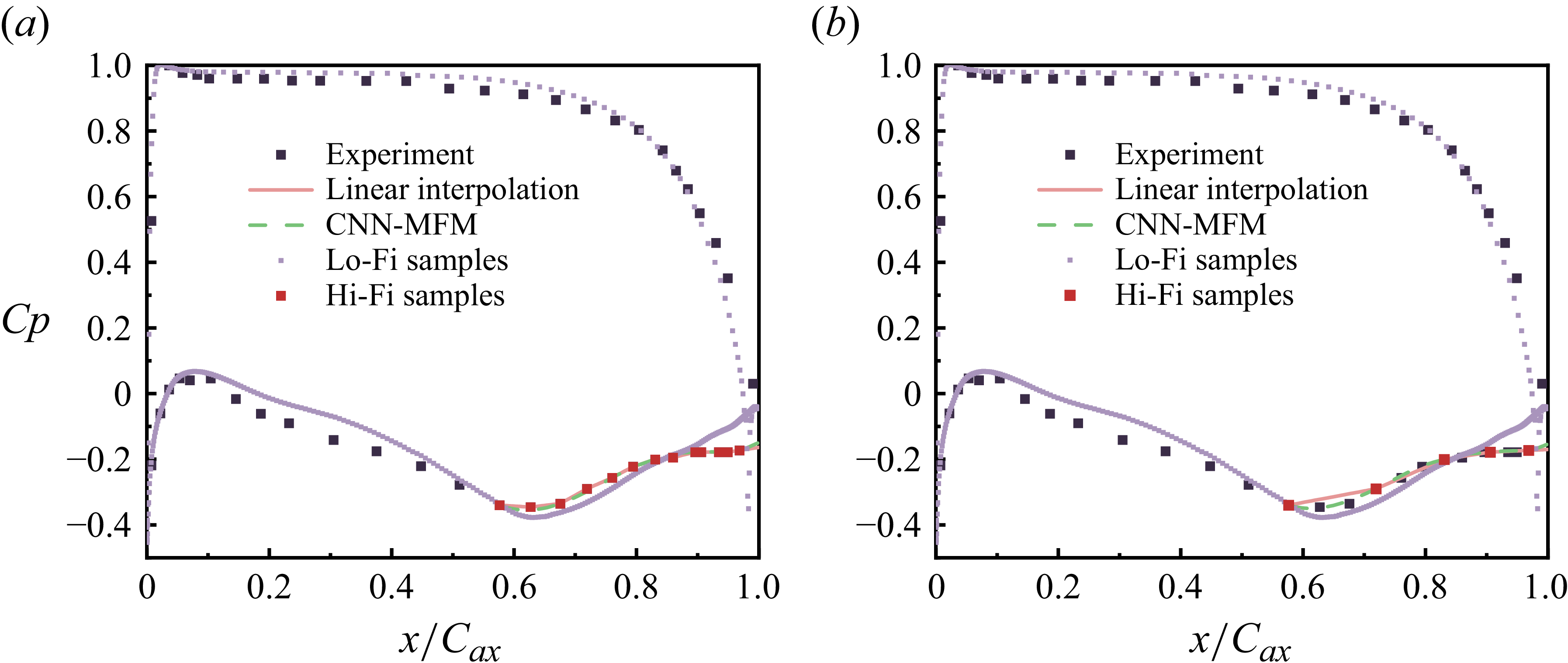
Comparison of pressure distribution predictions by the convolutional neural-network-based multi-fidelity model (CNN-MFM) and linear interpolation using different amounts of Hi-Fi data. (a) Dense Hi-Fi samples. (b) Sparse Hi-Fi samples.

In the data assimilation process, the quality of the observation data has a direct impact on the accuracy and efficiency of assimilation. However, in practical cases, Hi-Fi data are often limited in quantity and sparsely distributed. This issue becomes particularly pronounced when surface quantities such as the pressure coefficient and wall shear stress or flow-field variables such as velocity components are selected as observation data, since the available Hi-Fi data usually cannot be directly mapped onto the RANS computational grid. Under such circumstances, relying solely on simple linear interpolation or projection of sparse Hi-Fi data is often insufficient to provide synthetic observations of adequate accuracy, thereby constraining the overall performance of the assimilation. To address this issue, we adopt a multi-fidelity data fusion strategy based on CNN, as proposed in Chen, Gao & Liu (Reference Chen, Gao and Liu2022), which leverages the complementary information between Lo-Fi RANS data and the limited Hi-Fi data to generate synthetic observations with satisfactory accuracy. The Lo-Fi RANS fields, although affected by inherent model-form bias, are computationally efficient and capture the overall physical trends of the flow while the Hi-Fi measurements serve as local corrections, anchoring the model to trusted reference values. By combining them, the CNN learns spatially varying relationships between the two fidelity levels and produces improved predictions of the quantities of interest. Taking the pressure distribution as an example, it is defined as
 \begin{equation} c_{p,x}=\frac {p_{x}-p_{2}}{p_{t1}-p_{2}} ,\end{equation}
where
 $p_{t1}$
is the inlet total pressure,
 $p_{2}$
is the exit static pressure and
 $p_{x}$
is the static pressure on the blade.
Figure 3(a) shows that the results of the CNN-based multi-fidelity aggregation model (CNN-MFM) on the RANS grid exhibit good agreement with the Hi-Fi reference data By contrast, data obtained by linearly interpolating the Hi-Fi data onto the RANS grid can achieve comparable accuracy only when the Hi-Fi data are densely distributed; when the Hi-Fi data are sparse, the interpolation results often fail to meet the required accuracy, as illustrated in figure 3(b). The prediction errors of the linear interpolation and CNN-MFM approaches at the Hi-Fi locations were evaluated using the root-mean-square error, defined as
 \begin{equation} \varepsilon (q)=\sqrt {\frac {1}{N}\sum _{i=1}^N\left (q_i^{\textit{pred}}-q_i^{\textit{ref}}\right )^2} ,\end{equation}
where N is the number of Hi-Fi sampling points,
 $q_i^{\textit{pred}}$
denotes the predicted value obtained from the two methods and
 $q_i^{\textit{ref}}$
is the corresponding reference Hi-Fi value.
The quantitative comparison, summarised in table 1, further highlights this behaviour: when the Hi-Fi data are sufficiently dense, linear interpolation performs as well as, or even slightly better than, the MFM approach in this training case; however, as the Hi-Fi data become sparse, the error of the linear interpolation increases sharply, whereas the MFM approach maintains a relatively low error. This limitation of linear interpolation is particularly pronounced when the relationship between the low- and high-fidelity data is strongly nonlinear, while the MFM approach can still achieve predictions much closer to the Hi-Fi results by effectively utilising the global trend captured by the Lo-Fi data together with the local corrections provided by the Hi-Fi data. Consequently, in cases where Hi-Fi data are spatially sparse, the CNN-MFM can generate broader and more accurate synthetic observations, enhancing the flexibility of observation placement during data assimilation. Furthermore, it enables subsequent optimisation of observation data selection in conjunction with different assimilation settings such as ensemble size and state-vector dimension, thereby improving both the accuracy and efficiency of the data assimilation process by fully exploiting the complementary information from multi-fidelity data sources.
Comparison of prediction errors
 $\varepsilon$
at Hi-Fi locations for the linear interpolation and CNN-MFM approaches under different Hi-Fi data densities.

2.3.2. Selection of observation data informed by observability Gramian analysis
Based on the observability Gramian analysis method used in Franceschini, Sipp & Marquet (Reference Franceschini, Sipp and Marquet2020), the controllability of the correction to the production term in the baseline model is evaluated. Specifically, this analysis aims to determine whether the current correction approach can yield an accurate prediction of the mean-flow using only limited observation data.
The observability Gramian analysis begins by constructing a linear mapping operator
 $\mathcal A$
that relates variations in the correction parameters
 $\delta {\boldsymbol{\tilde f}}= (\delta a_i,\delta b_i,\delta c_i )$
to corresponding variation on the measurements
 $\delta {\boldsymbol{\tilde m}}$
, as expressed by
 \begin{equation} \delta {\boldsymbol{\tilde m}} = {\mathcal A}\delta {\boldsymbol{\tilde f}} .\end{equation}
In this study, the correction parameters correspond to input features that are all dimensionless. We further apply a logarithmic transformation to these features to reduce scale disparity while preserving physical meaning and improving numerical stability. Consequently, the correction parameters serve as dimensionless weights of comparable magnitude, and the perturbations
 $\delta {\boldsymbol{\tilde f}}$
applied to these parameters are of the same order. Therefore, different terms in
 $\delta {\boldsymbol{\tilde f}}$
are directly comparable in the Gramian analysis and are not biased by differences in physical units.
To analyse the parameter sensitivity, singular value decomposition is applied to
 $\mathcal A$
, resulting in
 \begin{equation} {\mathcal A} = {\boldsymbol {U}}\varSigma {{\boldsymbol {V}}^T} .\end{equation}
Here,
 $\boldsymbol{U}$
is an orthogonal matrix composed of the left singular vectors, V is an orthogonal matrix composed of the right singular vectors and
 $\varSigma$
is a diagonal matrix whose diagonal entries are all non-negative real numbers. These singular values can be obtained by solving the following eigenvalue problem:
 \begin{equation} {{\mathcal A}^T}{\mathcal A}\delta {{\boldsymbol{\tilde f}}_i} = \lambda _i^2\delta {{\boldsymbol{\tilde f}}_i} ,\end{equation}
where the positive eigenvalues are ranked by decreasing order, which means
 $\lambda _i^2 \ge \lambda _{i + 1}^2$
. This leads to
 \begin{equation} \delta {\boldsymbol{\tilde m}} = {\mathcal A}\delta {\boldsymbol{\tilde f}} = {\mathcal A}\sum \limits _i {{\alpha _i}} \delta {{\boldsymbol{\tilde f}}_i} = \sum \limits _i {{\alpha _i}} {\lambda _i}\delta {{\boldsymbol{\tilde m}}_i} = {\lambda _0}\sum \limits _i {{\alpha _i}} \frac {{{\lambda _i}}}{{{\lambda _0}}}\delta {{\boldsymbol{\tilde m}}_i}. \end{equation}
For a given
 $\delta {\boldsymbol{\tilde f}}$
, the corresponding impact on the observation space is projected via (2.9). If there are strong separation between the eigenvalues, it indicates that the current correction model can retain stability and effectiveness even with sparse observation data. Conversely, if all eigenvalues are of similar magnitude, it implies that the correction model is more flexible and requires more observation data for sufficient constraints to avoid instability.
2.4. Design of input features and training cases
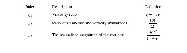
Section 2.1 defines the correction expression based on an RBF form, although the specific input features used to calculate the exact correction values are yet to be determined. Since the choice of input features significantly affects model applicability, incorporating relevant flow physics into the input features design improves the model’s ability to capture diverse flow characteristics. Meanwhile, limiting the number of features helps reduce model complexity, thereby promoting better generalisation. Our selection of input features draws on Singh et al. (Reference Singh, Medida and Duraisamy2017), who considered key quantities involved in the computation of eddy viscosity in the original S–A model. Using such established and physically meaningful features allows us to better isolate and demonstrate the effectiveness of the proposed RBF-based correction expression itself. We further refine the selection based on the feature importance analysis from our previous work (Gou et al. Reference Gou, Ye and Zou2025). The normalised Reynolds stress, which was ranked highest in contribution in our earlier analysis, was excluded here because its magnitude differs substantially from that of the other candidates, which could compromise the robustness of the correction expression. In addition, since the correction acts on the production term of the transport equation, it is not appropriate to include the ratio of the production to the destruction terms of the S–A model as an input feature. Considering both physical relevance and the desire for a compact and robust formulation, we therefore selected the next three most important features, which are listed in table 2. For numerical stability and to improve the representation within the RBF-based correction expression (2.5), the logarithm of each selected feature is used.
Input features selection aimed at separated-flow modelling.

After the input features are determined, the correction term in the form of RBF is introduced and integrated into the RANS solver, allowing the iterative correction to be accounted for. Moreover, the target flow variable for assimilation can be flexibly chosen from any quantity in the CFD calculation, depending on specific requirements. Importantly, since the structure of the RBF-based correction is fixed prior to training, the corrections determined by each ensemble member can be directly embedded into the RANS solver through parameter reading. As a result, there is no need to modify the solver for different cases, enabling simultaneous training across multiple flow scenarios. The correction models obtained from different training cases may take the same radial-basis-function form but exhibit different parameters. To highlight the trade-off between model simplicity and its ability to address diverse flow physics, and to examine the generalisation capability of a correction learned from limited data, we first train the model using a single case and then evaluate whether the resulting correction is applicable to other cases with similar flow characteristics. In principle, the same functional form of the correction can be applied with different coefficients for different flow regions or multiple training cases, allowing the model to account for a wider range of flow physics while maintaining a relatively simple structure.
Figure 4 illustrates the proposed turbulence modelling framework using RBF-based correction. In phase A, the specific input features for the correction model, along with the initial distributions of ensemble members, are first defined. The number of selected input features determines the number of parameters to be inferred using the EnKF method. Each parameter is assumed to follow an independent and identically distributed Gaussian distribution, from which samples are drawn to form the initial ensemble. The mean and variance of each distribution can be determined based on the spatial average and empirical standard deviation of the corresponding input features. This initialisation strategy is designed to ensure sufficient ensemble diversity while maintaining the stability of the updating process of the EnKF method. Upon completion of phase A, the functional form of the RBF-based correction is fully specified. This formulation is then embedded into the RANS solver, with the correction parameters dynamically retrieved at the beginning of each CFD run according to the state variables of the ensemble member, thus ensuring that each member yields a unique correction model. In phase B, the correction is integrated into the CFD calculation. The corrections are updated iteratively during the RANS iterations and applied at each step to modify the turbulence model predictions, thereby achieving numerical embedding of the correction model. Benefiting from the integration of the correction into the CFD calculation, the target variable used in the loss function can be flexibly defined. Furthermore, the RANS solver does not require additional modifications and is applicable to different test cases for the correction is embedded numerically in this phase, making it feasible to use multiple training cases simultaneously with a consistent computational framework. After the RANS simulation with modified S–A model is completed, phase C constitutes the main process of the EnKF method. It involves comparing the RANS predictions of each ensemble member with the observation data to compute the observation error covariance matrix. Based on this, the Kalman gain associated with the observation error covariance is calculated. Subsequently, the state variables of each ensemble member, including the parameters of the RBF, are updated using the Kalman gain. The updated correction expression is then re-integrated into the RANS solver, and phases B and C are repeated. The B–C iteration continues until convergence is achieved. In practice, convergence is determined either by the ensemble mean of the predicted flow variables approaching the observation data within the prescribed tolerance, or by the ensemble variance of the correction parameters becoming smaller than the observation error. The former criterion is particularly relevant when a relatively wide distribution in the state vector still produces very similar predicted flow fields, making the reduction of the parameter variance less indicative of convergence in the quantities of interest. Once convergence is reached, the mean of the ensemble state variables is taken as the final set of parameters for the RBF, representing the learned corrected model. This modified model can then be tested across other relevant flow cases to assess its generalisation performance.
Schematic of a model-consistent turbulence modelling framework with RBF-based corrections and ensemble-based assimilation, consisting of the following three phases: (a) initialisation of the ensemble by randomly sampling the parameters of the RBF; (b) embedding of the correction into the RANS solver, including both structural incorporation of the RBF formulation and numerical embedding through iterative updating of the correction values during the RANS simulation; (c) the RBF parameters are updated based on the observation data, and the updated parameters are re-embedded in phase B, forming a closed-loop FIML process.

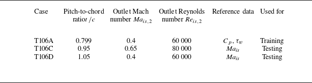
Overview of the training and testing cases including the Pitch to chord ratio (t/c), Mach numbers (Ma) and Reynolds numbers (Re).

Sketch of the T106A blade geometry and domain boundaries.

3. Case set-up
The T106 low pressure turbine (LPT) cascade, representative of a high lift and aft-loaded blade and corresponding to the mid-span section of the PW2037 LPT rotor (Stadtmüller & Fottner Reference Stadtmüller and Fottner2001), is chosen for training and testing. This profile has been extensively studied and exhibits a range of flow separation behaviours under different operating conditions, providing a rich database (Stadtmüller Reference Stadtmüller2001; Ye Reference Ye2008; Michálek et al. Reference Michálek, Monaldi and Arts2012; Michelassi et al. Reference Michelassi, Chen, Pichler and Sandberg2015; Sandberg et al. Reference Sandberg, Michelassi, Pichler, Chen and Johnstone2015 ; Wang et al. Reference Wang, Sui, Zhang, Xiang and Zhao2018) for model development and validation. In the training phase, the RBF-based FIML framework is applied to the T106A-EIZ case (Stadtmüller Reference Stadtmüller2001; Michelassi et al. Reference Michelassi, Chen, Pichler and Sandberg2015; Sandberg et al. Reference Sandberg, Michelassi, Pichler, Chen and Johnstone2015; Wang et al. Reference Wang, Sui, Zhang, Xiang and Zhao2018) to derive the correction model. This configuration has a pitch-to-chord ratio of 0.799 and a chord length of 100 mm, with an inlet flow angle of 46.1
 $^\circ$
, measured counterclockwise from the horizontal at the leading-edge stagnation point. The computational domain and geometry of T106A are shown in figure 5. A no-slip condition is imposed on the blade surfaces, periodic boundary conditions are used in the pitch-wise direction and the inlet is specified with total temperature and pressure aligned with the inflow angle. The computational mesh used in this study has been verified for grid independence, and the first grid point from the wall satisfies
 ${y^ + } \lt 0.8$
, ensuring that discretisation error is significantly smaller than the turbulence modelling error. The same mesh is used consistently during RANS calculations with both the baseline and corrected model to ensure results are grid-independent. Simulations for T106A are conducted at the isentropic Reynolds number Re = 60 000, where flow separation occurs on the suction side near the trailing edge, but is entirely missed by the baseline S–A model. For model testing, we employ the T106C and T106D-EIZ cases. In the baseline S–A simulations, the T106C case exhibits no separation, while the T106D-EIZ case already shows open separation. These test cases are chosen to assess the capability of the trained correction model in addressing different flow behaviours predicted by the baseline model. Table 3 summarises the operating conditions of all training and testing cases, along with the available Hi-Fi reference data.
4. Results
4.1. Flow around the T106A: FIML-Direct for RBF-based correction
Based on the correction region identified in Gou et al. (Reference Gou, Ye and Zou2025), the FIML-Direct framework is applied to T106A by introducing correction terms within the selected regions. Specifically, the viscosity ratio and pressure gradient magnitude derived from the baseline S–A model are used as two-dimensional features for clustering via GMMs. The cluster characterised by higher viscosity and lower pressure gradient magnitude is identified as the correction region, corresponding to the viscous-dominated near-wall zones where RANS model discrepancies are most pronounced. The activated correction region for T106A is illustrated in figure 6. The final distributions of the parameters in (2.5) are inferred using the EnKF method, leading to RANS predictions that better approximate the true flow field. The specific parameter settings for constructing the initial ensemble in the field inversion process are detailed in Appendix A. Given the limited availability of observation data, the final model may exhibit increased prediction error (Zhang et al. Reference Zhang, Xiao, Luo and He2022). To address this, the multi-fidelity data fusion method described in § 2.3.1 is employed. By combining sparse experimental data with load distribution results computed from the baseline model, synthetic observations on the RANS mesh corresponding to the T106A case are generated, as shown in the CNN-MFM result in figure 3(a).
Identification of the correction region using GMM-based clustering for T106A. The viscosity ratio and pressure gradient magnitude from the baseline S–A model are used as two-dimensional clustering features. The region with higher viscosity ratio and lower pressure gradient magnitude is where the correction expression is activated.

To assess the observability of the RBF-based correction parameters from the available observations, the observability Gramian derived from linear systems theory is employed in this study. The turbulence model augmented with correction terms is linearised around the steady RANS solver, enabling the construction of the observability Gramian matrix. The eigenvalue spectrum of this matrix, shown in figure 7, reveals a rapid decay, indicating that the system is sensitive to only a limited number of perturbation directions. Under sparse observational data, this low-rank characteristic helps mitigate overfitting in unobservable directions, thereby promoting stable and efficient convergence of the calculation results of the modified model toward reliable state reconstruction. As a result, the favourable conditioning revealed by the Gramian analysis makes the assimilation outcome relatively insensitive to the sparsity of the available observations, thereby improving the robustness and stability of the model correction under conditions of limited measurements.
Comparison of different synthetic observations generation methods during the data assimilation process.

Eigenvalue spectrum
 $(\lambda_i/\lambda_0)^2$
of the observability Gramian versus the mode index
 $i$
, indicating strong separation between the eigenvalues with the RBF-based correction.

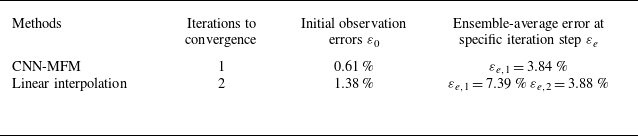
When generating synthetic observation data, table 4 compares the impact of using CNN-MFM versus linear interpolation on the data assimilation process under conditions of sparse Hi-Fi data. Two types of errors are evaluated. The observation error
 $\varepsilon _{0}$
quantifies the discrepancy between the synthetic observations and the reference data, while the ensemble-average error
 $\varepsilon _{e}$
measures the deviation between the ensemble-mean prediction and the reference data at each iteration step. Both are defined as
 \begin{align} \varepsilon =\sqrt {\frac {1}{N}\sum _i\left(C_p^{\textit{pred}}(x_i)-C_p^{\textit{ref}}(x_i)\right)^2} ,\end{align}
where
 $C_p^{\textit{ref}}$
represents the reference pressure coefficient obtained from the CNN-MFM model trained with dense Hi-Fi samples at 157 grid points from
 $x/C_{ax}=0.597$
to
 $x/C_{ax}=1$
. All model prediction errors for T106A presented in the following sections are computed based on this same definition. Specifically, when Hi-Fi data are spatially sparse, the linear interpolation method fails to accurately represent the true observation data distribution, resulting in higher initial observation errors. Moreover, due to the rigidity of the correction model, not all observations can be effectively sensed and corrected. Figures 8 and 9 show the ensemble-based data assimilation results using synthetic observations generated by linear interpolation and CNN-MFM respectively under different initial observation error conditions. While the ensemble-average errors eventually converge to similar levels in both methods, using linearly interpolated observations leads to slower convergence, as more iterations are required for the ensemble mean of the predicted flow variables to approach the observation data within the prescribed tolerance. In the present study, a relative difference of 5 % between the predicted and observed flow variables was adopted as the convergence threshold. Consequently, given the differences in initial observation errors and the required number of iterations, CNN-MFM demonstrates a greater ability to extract complementary information from multi-fidelity datasets, particularly when generating observations from reference data with strong nonlinearities, such as velocity distributions in separated flows. This enables the construction of observation data that are better suited to high-accuracy requirements. To further leverage the advantages of multi-fidelity data fusion, future work may explore other alternative fusion methods. Additionally, by integrating the predictive variance from the multi-fidelity models into the observation error term of the EnKF framework, it is possible to account for spatially varying observation uncertainties. This could enable more adaptive Kalman gain updates and provide improved guidance for parameter tuning and convergence behaviour in ensemble-based data assimilation.
Distribution of ensemble members during data assimilation with linearly interpolated synthetic observations. (a) Iteration 1. (b) Iteration 2.

Distribution of ensemble members during data assimilation with CNN-MFM synthetic observations for iteration 1.

Convergence assessment of the EnKF data assimilation for T106A.

Convergence process of the EnKF data assimilation for T106A. (a) Iteration 0. (b) Iteration 1.

Therefore, the interpolated results obtained from the CNN-MFM method, as shown in figure 3(a), are ultimately adopted as the observation data in this study. Specifically, when the pressure coefficients at 111 grid points from
 $x/{C_{ax}} = 0.6$
to
 $x/{C_{ax}} = 0.968$
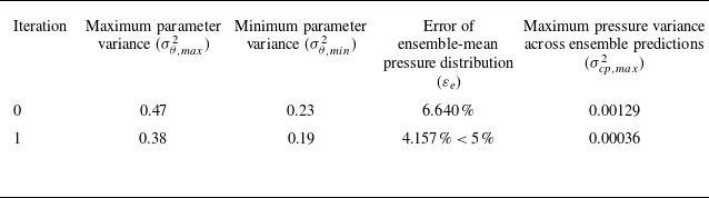
are used as the assimilation targets, the convergence process is illustrated in figure 10. In this figure, the thin solid lines represent the results of ensemble members, the dashed line indicates the ensemble average at each iteration step, the black dots denote the experimental data from Stadtmüller (Reference Stadtmüller2001) and the thick solid line corresponds to the prediction from the original model. Under the current assimilation parameter settings, the error of the ensemble-mean pressure distribution decreases rapidly after the first iteration and falls below the prescribed observation tolerance, as shown in table 5. Meanwhile, the ensemble variance of the RBF coefficients
 $\boldsymbol{\theta }=\begin{bmatrix}a_1,a_2,a_3,b_1,b_2,b_3,c_1,c_2,c_3\end{bmatrix}^{\mathrm{T}}$
also decreases but remains relatively broad, indicating that parameter convergence is slower than that of the predicted flow field. For the present training case, different RBF-based corrections can nevertheless produce very similar flow-field predictions. This observation indicates that the assimilation problem is relatively robust under the adopted low-dimensional and locally activated parameterisation, in the sense that different realisations of the correction can lead to consistent flow-field responses. Such robustness suggests that the correction acts as a smooth and bounded modulation of the model response, allowing the dominant discrepancies to be identified efficiently without requiring large or highly nonlinear parameter updates. While the details of preliminary trials with different initial ensemble distributions are not shown in this study, the results suggest that, for the relatively simple flow configuration and modest model-form discrepancy considered here, the assimilation outcome is largely insensitive to the choice of the initial ensemble. In more complex separated-flow cases with stronger nonlinearities and larger discrepancies, however, the assimilation result may become more sensitive to the choice of the initial ensemble. The ensemble-averaged state variables at the final iteration are then taken as the practically converged correction. When these parameters are substituted into the RANS solver, the resulting loading distribution is shown in figure 11. It can be observed that the predictions of RBF-augmented S–A model obtained after the EnKF data assimilation exhibit significantly better agreement with the DNS results reported by Sandberg et al. (Reference Sandberg, Michelassi, Pichler, Chen and Johnstone2015), compared with the original uncorrected model.
Distribution of pressure coefficient for T106A.

Distribution of wall shear stress for T106A.

An analysis of the wall shear stress distribution presented in figure 12 indicates that, for the RBF-augmented model, the predicted wall shear stress on the blade surface decreases below zero near at
 $x/{C_{ax}} = 0.8$
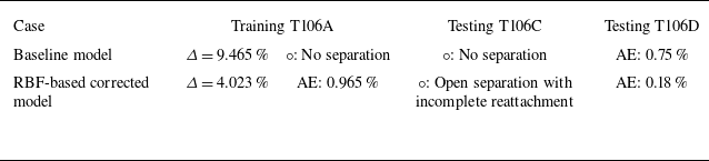
, suggesting the onset of boundary-layer separation at this location. The shear stress remains negative up to the trailing edge, which is consistent with the open separation observed in the DNS results under low inflow turbulence intensity conditions (Michelassi et al. Reference Michelassi, Chen, Pichler and Sandberg2015; Wang et al. Reference Wang, Sui, Zhang, Xiang and Zhao2018). This separation behaviour is also evident in figure 13, which shows the Mach number contours and streamlines. Consequently, even using only the pressure coefficient distribution as observations can improve the prediction of the friction coefficient in the training case and enhance the capture of the separation region. This indicates that the learned correction model identifies the intrinsic deficiencies of the original turbulence model to some extent, rather than merely fitting the
 $C_{p}$
curve. This also lays a foundation for the modified model to still improve the prediction accuracy in more complex separated flows in the future. The final parameters of the correction expression in (2.5) obtained from the data assimilation process for this training case are as follows:
 \begin{equation}\begin{aligned} &{a_1} = 0.461, &{a_2} = 1.265, &\quad{a_3} = 0.379,\nonumber\\ &{b_1} = - 3.136, & {b_2} = 0.818, & \quad{b_3} = 2.870,\nonumber\\ &{c_1} = - 3.216, &{c_2} = 5.424, &\quad{c_3} = 1.693. \end{aligned}\end{equation}
To assess the generalisation capability, the RANS solver with the embedded correction expression is further applied to the validation cases.
Mach number contours for T106A: (a) original model and (b) RBF-augmented model.

Comparison of model predictions for test cases.:(a) T106C; (b) T106D.

4.2. Validation of the RBF-augmented turbulence model
The RBF-augmented model, embedded into the RANS solver in the same manner as used during the training phase, is further applied to simulate the T106C and T106D cases. The loading distributions by the original S–A model and the corrected model are shown in figure 14. At this stage, the loading distribution is analysed using the isentropic Mach number, which is specifically defined as
 \begin{equation} Ma_{is,x}=\sqrt {\frac {2}{\kappa -1}\boldsymbol{\cdot }\left [\left (\frac {p_{t1}}{p_x}\right )^{\frac {\kappa -1}{\kappa }}-1\right ]} .\end{equation}
where
 $\kappa$
is the ratio of specific heats, taken as 1.4. It can be seen that it is still calculated based on the blade surface static pressure, consistent with the physical meaning represented by the observation data in the training case. For the T106C case, there is no separation phenomenon in the calculation results of the original model, whereas the corrected model accurately captures the onset of separation, as evidenced by the flat portion of the curve, and provides an improved prediction of the partially reattached flow downstream. In the T106D case, due to its relatively large pitch-to-chord ratio, the original model predicts open separation but underestimates the separation onset compared with the LES results. The corrected model retains the capability to predict large-scale separation while simultaneously improving the accuracy of the separation onset location, as illustrated by the wall shear stress distribution in figure 15. Specifically, the absolute error of the predicted separation point, defined as the absolute difference between the non-dimensional separation locations obtained from the predicted and reference results, is reduced from 0.75 % to 0.18 % after applying the RBF-based correction. A comprehensive comparison of all training and testing cases, including both the baseline and corrected models, is summarised in table 6.
Comparison of prediction performance between the baseline RANS model and the RBF-based corrected model across different cases. (
 $\varDelta$
: pressure distribution error,
 $\circ$
: flow separation behaviour, AE: predicted separation location absolute error.).

Distribution of wall shear stress for T106D. Here, MOD–SA and ORI–SA correspond to the Modified S–A and Original S–A models, respectively.

Figure 16 compares the Mach number contours predicted by the original and augmented models for the T106C case. The correction expression trained on the T106A case significantly improves the capability of the original S–A model in capturing the large-scale separation behaviour when directly applied to T106C. To further elucidate the physical effect of the correction, figure 17 presents the contours of the eddy-viscosity difference, defined as the local value predicted by the augmented model minus that from the baseline model, for the two test cases. In both cases,
 $\Delta V_t$
is predominantly negative in the separated shear-layer regions, indicating that the RBF-based correction tends to reduce the eddy viscosity locally where the baseline S–A model is known to overpredict it. The reduction is mainly observed downstream of the suction-side separation bubble, whereas the attached boundary-layer regions are largely unaffected. Around the edges of the separated regions, the eddy viscosity is locally increased in one case and decreased in the other, reflecting the differing predictions of the baseline S–A model, where T106C remains largely attached and T106D already develops an open separation. Such a localised decrease in the eddy viscosity aligns with the physical understanding that reduced eddy viscosity diminishes the stabilising effect on the shear layer, thereby promoting an earlier onset and a larger extent of separation. Notably, the consistent correction trend observed in both cases provides physical insight into how the RBF-based corrections can help address the well-recognised challenge that the baseline S–A model faces in accurately predicting flow separation, supporting the interpretation that the inferred correction captures a transferable, physically meaningful trend, namely the need for localised eddy-viscosity reduction in separation-prone shear layers, and not merely an overfit to the training case. Considering that the proposed correction expression is derived from a single training case with prominent flow separation and features a compact and efficient form, the current model’s applicability remains limited to flows with similar characteristics. Nevertheless, due to its computational efficiency and ease of implementation, the correction framework can be further extended to broader flow regimes by training with additional representative cases that exhibit diverse flow features. Appropriately enriching and designing the input features or employing transfer learning techniques to fine tune the existed correction models may also improve its generalisation capability across different flow scenarios.
Mach number contours for the T106C: (a) original model and (b) RBF-augmented model.

Contours of the eddy-viscosity difference
 $\Delta \nu _t=\nu _{t,{aug}}-\nu _{t,{base}}$
showing the local effect of the RBF-based correction on the separated shear-layer regions: (a) T106C; (b) T106D.

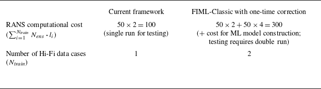
Table 7 compares the computational cost associated with the corrected model obtained using the present method and that of a previous model under the FIML-Classic framework, which here denotes the one-time field-correction approach used in our earlier work. This previous model achieved similar improvements on the same cases. The total number of RANS calculations required during the data assimilation process using the EnKF method depends on the number of training cases with Hi-Fi data
 $N_{\textit{train}}$
, the ensemble size
 $N_{\textit{ens}}$
and the number of iterations
 $l_{i}$
required for convergence for each training case. The total cost can thus be expressed as
 \begin{equation} \text{Total RANS calculations}=\sum _{i=1}^{N_{\textit{train}}}N_{\mathrm{\textit{ens}}}\boldsymbol{\cdot }l_{i} .\end{equation}
Specifically, for the three cases involving flow separation in this study, the model-consistent turbulence modelling framework with RBF-based corrections and ensemble-based assimilation requires
 $ 50 \times 2 = 100$
RANS calculations, while the FIML-Classic framework requires
 $ 50 \times 2 + 50 \times 4 = 300$
RANS calculations. The reduced computational load in this part during the data assimilation process is mainly achieved through the improvement of the model’s generalisation ability. In addition, when the RBF is not used, it is also necessary for additional ML model training, further increasing the cost associated with constructing the correction model. During model testing on unseen cases, the online use of a learned correction from either the adjoint-based approach or the present RBF-based method requires only a single RANS solution for each target case. In the classic framework used for comparison in this study, which employed a one-time-correction approach, each new flow configuration required two RANS runs: one to obtain the input features from the baseline solution and another to solve the RANS equations with the corrected closure. In contrast, the RBF-based correction embedded directly into the CFD solver does not need to calculate the input features separately and enables the direct evaluation of the RBF-augmented turbulence model. Therefore, the proposed correction framework demonstrates clear advantages in both computational efficiency and model generalisation, making it more suitable for practical engineering applications involving complex separated flows.
Comparison of the current framework and FIML-Classic in terms of computational complexity.

The integration of the correction model into the CFD calculations enables the influence of iterative corrections to be incorporated during the model training process. By selecting appropriate input features, this approach facilitates the construction of explicit correction expressions that dynamically respond to variations in flow characteristics, thereby enhancing the model’s generalisation capability. In summary, the current RBF-based correction model can effectively improve the prediction of separated flows. Its integration with the RANS solver allows direct application to test cases beyond the training set, reducing the computational cost of testing. Moreover, the iterative correction method, which adapts to the evolving input features during RANS simulations, enables improved predictions of turbine cascade flows with different geometries and Reynolds numbers when only a single Hi-Fi dataset is available. Although only minor corrections are required for the current training case, the constructed model can effectively improve other flows with similar features but greater complexity, indicating that it captures the relevant physical characteristics to a certain extent. This limited generalisation is enabled by the structured and compact form of the correction, which acts as a transferable baseline within a related class of flows. We believe that this generalisation capability ensures the applicability of the proposed method to other cases with stronger nonlinearities, or allows the direct transfer of the correction model to more complex separated-flow scenarios. These findings provide a basis for the further development of correction models through systematic extension or refinement of the current formulation, with a general structure complemented by flow-specific enhancements (Yang et al. Reference Yang, Shan, Yang and Zhang2025), enabling improved predictions for increasingly complex flow conditions while preserving a controlled level of generalisation.
5. Conclusion
In this study, a correction term based on the RBF formulation is applied flexibly to the production term of the S–A one-equation turbulence model within adaptively identified correction regions. By integrating this correction expression with a CFD solver, a dynamic correction model is established that evolves with changes in input features. This method improves the predictive accuracy for flows with separation characteristics, leading to the following conclusions.
-
(i) The proposed RBF-based iterative correction model accounts for flow-dependent variations during the RANS calculation. It has been shown that training with Hi-Fi data from a single case enables accurate predictions for other cases with similar separation characteristics, demonstrating the model’s generalisation capability. Furthermore, this correction framework is extendable to other complex flow scenarios, providing an efficient approach for improving RANS model predictions in a broader range of applications.
-
(ii) The inversion of parameters in compact-form RBF not only reduces computational cost during the training phase by enhancing model generalisation, but also eliminates the need for training separate ML models. The resulting correction model can be directly deployed in flow prediction without requiring input features to be recomputed from the baseline model, further enhancing the efficiency of model construction and application.
-
(iii) The use of multi-fidelity data fusion enables the construction of synthetic observations that improve the effective utilisation of Hi-Fi data, increase the availability of observations meeting higher accuracy requirements and reduce observation errors. When combined with the inversion of parameters for RBF instead of correcting the entire spatial distribution, this approach effectively reduces the dimensionality of the assimilation parameters and accelerates the convergence of the data assimilation process.
Acknowledgements
This study was supported by the National Science and Technology Major Project (No. J2019-II-0012-0032). The support is gratefully acknowledged.
Declaration of interests
The authors report no conflicts of interest.
Appendix A. Integration of the EnKF method with radial-basis-function-based correction
This appendix provides a detailed description of the integration between the EnKF method and the correction model expressed in RBF form. During the construction of the initial ensemble members, since the spatial distribution of the correction term applied to the source term is represented using a fixed RBF expression, it is necessary to generate the initial ensemble members by performing multiple random samplings of the undetermined coefficients in the RBF formulation. Based on prior experience of constructing the input features, each ensemble member is generated by sampling nine independent random variables, each following a normal distribution. The mean values of these distributions are chosen with reference to the spatial average of the corresponding input features within the correction region, as computed from the converged flow field of the baseline model. To improve the covariance adjustment capability of the EnKF method under small ensemble size conditions, the weights of the RBF corresponding to different features are sampled from normal distributions with a standard deviation of 1.0, while the remaining parameters follow normal distributions with a standard deviation of 0.5. The sampled parameters are then substituted into the fixed RBF expression, guided by the input features of the baseline model. To ensure the physical plausibility and stability of the correction, the resulting magnitude of the synthetic correction field represented by each ensemble member is constrained to within
 $\pm 3$
. Therefore, for the RBF expression
 $\beta ( {{\eta _1},{\eta _2} \ldots } ) = 1 - \sum \nolimits _{i = 1}^n {{a_i}} {e^{ -({{{{ ( {{\eta _i} - {b_i}} )}^2}}}/{{2{c_i}^2}})}}$
selected in this paper, the initial ensemble members for each parameter are generated according to the following distributions:
 \begin{equation} \begin{array}{l} {a_i} \sim N\left ( {\overline {{a_i}} ,1} \right ),\\ {b_i} \sim N\left ( {\overline {{b_i}} ,{{0.5}^2}} \right ),\\ {c_i} \sim N\left ( {\overline {{c_i}} ,{{0.5}^2}} \right ), \end{array} \end{equation}
where the parameter
 $\overline {{a_i}}$
can be set to 0, and
 $\overline {{b_i}}$
and
 $\overline {{c_i}}$
can be determined based on the mean and variance of the corresponding input features within the modification region, as computed from the results of the original model.
The specific implementation procedure for the ensemble-based model learning is summarised below.
(a) Prediction step
The complete state vector is computed by substituting either the initial ensemble member distribution or the state vector from the previous step into the RANS solver, as expressed in (A2)
 \begin{equation} {{\boldsymbol {x}}_i}^f = \left (\!\! \begin{array}{l} {{\boldsymbol {C}}_{\!p}}\\ {\boldsymbol {A}} \end{array} \!\!\right )\! ,\end{equation}
where the vector
 ${\boldsymbol {C}}_p$
represents the prediction of observation data for an individual ensemble member. The vector
 $\boldsymbol {A}$
contains the parameters for turbulence model correction using RBF and
 ${\boldsymbol {A}} = { ( {{a_1},{a_2}, \ldots {a_n},{b_1},{b_2}, \ldots {b_n},{c_1},{c_2}, \ldots {c_n}} )^{{T}}}$
To compute the covariance matrix in the analysis step, the ensemble mean is obtained as
 \begin{equation} {\overline {\boldsymbol {x}} _n} = \frac {1}{N}\sum \nolimits _{i = 1}^N {{\boldsymbol {x}}_i^f} \end{equation}
where
 $n$
denotes the current iteration step.
(b) Analysis step
The prediction error and the Kalman gain matrix are calculated in the analysis step. The observation error is given by
 ${{\boldsymbol{\omega }}_i} = {{\boldsymbol {y}}_{{\boldsymbol {obs}}}} - {\boldsymbol {B}}{{\boldsymbol {x}}_i}^f$
, where
 ${\boldsymbol {y}}_{{\boldsymbol {obs}}}$
represents the observation data derived from Hi-Fi data and
 $\boldsymbol {B}$
is the matrix that maps the state space to the observation space. In the present work,
 ${\boldsymbol {B}} = ( {{{\boldsymbol {I}}_l} {{\boldsymbol {0}}_{l \times (m - l)}}} )$
, where
 $l$
and
 $m$
denote the number of observation data points and the dimension of the state vector, respectively, with
 $m - l = 9$
. The observation error covariance matrix can be written as
 \begin{equation} {\boldsymbol {R}} = \frac {1}{{N - 1}}({{\boldsymbol{\omega }}_{\boldsymbol {1}}}{{\boldsymbol{\omega }}_{\boldsymbol {2}}} \ldots {{\boldsymbol{\omega }}_{\boldsymbol {N}}}{\boldsymbol {)(}}{{\boldsymbol{\omega }}_{\boldsymbol {1}}}{{\boldsymbol{\omega }}_{\boldsymbol {2}}} \ldots {{\boldsymbol{\omega }}_{\boldsymbol {N}}}{)^T} .\end{equation}
To avoid constructing a high-dimensional covariance matrix, the true covariance matrix is approximated using the sample covariance matrix written as
 \begin{equation} {\boldsymbol {P}} = \frac {1}{{N - 1}}\sum \nolimits _{i = 1}^N {\left({\boldsymbol {x}}_i^f - {{\overline {\boldsymbol {x}} }_n}\right){{\left({\boldsymbol {x}}_i^f - {{\overline {\boldsymbol {x}} }_n}\right)}^T}} .\end{equation}
Considering potential spurious correlations in the error covariance due to limited ensemble size, the adaptive covariance inflation technique from Luo et al. (Reference Luo, Stordal, Lorentzen and Nævdal2015) is employed. Thus, the Kalman gain matrix is given by
 \begin{equation} {\boldsymbol {K = P}}\!{{\boldsymbol {B}}^{\boldsymbol {T}}}{{\boldsymbol {\!(B{\kern-1pt}P}}{{\!\boldsymbol {B}}^{\boldsymbol {T}}}{\boldsymbol { + }}\bigl(1 + {\lambda ^l}\bigr){\boldsymbol {R)}}^{{\boldsymbol { - 1}}}} ,\end{equation}
where
 $1 + {\lambda ^l}$
is the inflation parameter. As shown in (A6), the Kalman gain quantifies the relative significance of prediction error in relation to observation error.
(c) Update step
Ensemble members are updated according to the Kalman gain using
 \begin{equation} {\boldsymbol {x}}_i^a = {\boldsymbol {x}}_i^f + {\boldsymbol {K}}\!\left({{\boldsymbol {y}}_i} - {\boldsymbol {Bx}}_i^f\right) ,\end{equation}
yielding the posterior distribution of the system state through ensemble statistics. After one iteration, the spatial distribution of the correction coefficients in the source term, obtained from the updated state vector, is treated as the prior distribution for the next iteration. This updated distribution is substituted into the RANS solver to perform the prediction step of the new iteration. The convergence of the ensemble member is assessed by examining either the ensemble mean of the predicted flow variables relative to the observation data or the ensemble variance of the correction parameters. Once the former is sufficiently close to the observation data or the latter falls below the prescribed observation error, the correction represented by the ensemble mean is regarded as adequately converged. Upon completion of this stage, the mean of the final state-vector samples is used as the correction model for further testing and validation on additional flow cases.