







1. Introduction
In this paper, we first consider the existence of ground state solutions to the following class of elliptic problems
 \begin{equation}
\left\{
\begin{aligned}
&-\Delta_{\mathbb{B}^N} u+V(x)u=f(u) \quad \hbox{in} \quad \mathbb{B}^N,\\
&u(x) \gt 0 \quad \mbox{in} \quad \mathbb{B}^N,
\end{aligned}
\right.
\end{equation}
where  $\mathbb{B}^N$ is the disc model of the Hyperbolic space and
 $\Delta_{\mathbb{B}^N}$ denotes the Laplace–Beltrami operator with
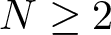
 $N \geq 2$,
 $V:\mathbb{B}^N \to \mathbb{R}$ and
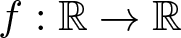
 $f:\mathbb{R} \to \mathbb{R}$ are continuous functions that satisfy some technical conditions.
Hereafter, we assume that the nonlinearity f is a continuous function with subcritical growth, that is, it satisfies the following set of assumptions:
(f1)
 $f(-t)=-f(t)$ for all
$t\in\mathbb{R}$ and
$f(t)=o(t)$ as t → 0.
(f2) There exists a constant
$q \in (2,2^*)$ such that
\begin{equation*}
\lim_{|t| \to +\infty} \frac{|f(t)|}{|t|^{q-1}}=0,
\end{equation*}where
$2^*=\frac{2N}{N-2}$ if
$N\geq3$ and
$2^*=\infty$ if N = 2.(f3) The function
$t\mapsto\frac{f(t)}{|t|}$ is decreasing and increasing in
$(-\infty,0)$ and
$(0,+\infty)$, respectively.(f4) There is a constant θ > 2 such that
$0 \lt \theta F(t) \leq f(t)t$,
$\forall t \not= 0$, where
$F(t)=\int_0^tf(s)ds$.


Over the past several decades, Problem (1.1), which is closely related to various geometrical issues, has been paid considerable attention by a great number of mathematicians. For instance, taking  $V(x)=\lambda\in\mathbb{R}$ for all
 $x\in \mathbb{B}^N$ and
 $f(t)=|t|^{p-2}t$ for each
 $t\in\mathbb{R}$ with
 $2 \lt p \lt 2^*$ in (1.1) into account, it arises in the considerations of the Crushin operator [Reference Alves and de Holanda2, Reference Beckner14], the Hardy–Sobolev–Maz’ya equation [Reference Castorina, Fabbri, Mancini and Sandeep23, Reference Castorina, Fabbri, Mancini and Sandeep24, Reference Mancini and Sandeep53] as well as in the prescription of Webster curvature on the Heisenberg group [Reference Ho44, Reference Ho45, Reference Salem and Gamara61]. Moreover, we would like to refer the reader to [Reference Bhakta and Sandeep18, Reference Carrião, Faria and Miyagaki20–Reference Carrião, Costa and Miyagaki22, Reference doÓ and da Costa32, Reference Ganguly, Gupta and Sreenadh35, Reference Ganguly and Sandeep37] and their references therein for some other interesting and meaningful results concerning the existence, uniqueness, regularity, symmetry, and non-degeneracy properties of nontrivial solutions.
When posed in the Euclidean space  $\mathbb{R}^N$, Problem (1.1) goes back to the nonlinear Schrödinger equation below
 \begin{equation}
-\Delta u+V(x)u=f(u) \quad \hbox{in} \quad \mathbb{R}^N,
\end{equation}
where Δ stands for the usual Laplacian operator in  $\mathbb{R}^N$. In light of the actual applications in mathematical and quantum physics, Bose–Einstein condensates as well as nonlinear optics, see e.g. [Reference Cazenave25, Reference Guo and Seiringer40, Reference Lieb, Seiringer and Yngvason49, Reference Seiringer62], equation (1.2) and its variants have been widely investigated by Berestycki and Lions [Reference Berestycki and Lions16, Reference Berestycki and Lions17], Bahri and Berestycki [Reference Bahri and Berestycki10], Bahri and Li [Reference Bahri and Li11], Bahri and Lions [Reference Bahri and Lions12], etc. We should emphasize here that one of the main challenges in studying semilinear elliptic equations like equation (1.2) in the whole space
 $\mathbb{R}^N$ comes from the lack of compactness due to the unboundedness of the domain, namely through the vanishing of mass in the sense of concentration-compactness principle of Lions [Reference Lions50, Reference Lions51]. For more related results, see [Reference Adachi and Tanaka1, Reference Alves and Shen5, Reference Alves and Thin7, Reference Cerami and Passaseo26, Reference Malchiodi52, Reference Musso and Pimentel55, Reference Szulkin and Weth66] and their references therein even if these references are far from exhaustive.
It is also interesting to contemplate equation (1.2) with respect to different ambient geometries, in particular, to observe how curvature properties affect the existence and nature of solutions. In the last decades, Mancini and Sandeep dealt with the analogous equation in the Hyperbolic space. More precisely, in the seminal paper [Reference Mancini and Sandeep53], they investigated the existence and uniqueness of finite energy-positive solutions of the following homogeneous elliptic equation
 \begin{equation}
-\Delta_{\mathbb{B}^N} u-\lambda u=u^{q-1} \quad \hbox{in} \quad \mathbb{B}^N,
\end{equation}
in the subcritical case for all  $\lambda \lt \frac{(N-1)^2}4$ and in the critical exponent case for
 $\frac{N(N-1)}{4} \lt \lambda\leq\frac{(N-1)^2}4$ with
 $N\geq4$. Moreover, they showed that equation (1.3) admits a positive solution for λ = 0 and
 $2 \lt q \lt 2^*$. These positive solutions are further verified to be unique, up to Hyperbolic isometries, except possibly for N = 2 and
 $\lambda \gt \frac{2(p+1)}{(p+3)^2}$. Subsequently, Bhakta and Sandeep [Reference Bhakta and Sandeep18] reached the priori estimates, existence/nonexistence of radial sign-changing solutions of (1.3). Let us introduce some delicate results in [Reference Ganguly and Sandeep36] concerning the existence of infinitely many sign-changing solutions for
 $N\geq7$ and it remains open for
 $N\leq6$. In [Reference Bonforte, Gazzola, Grillo and Vázquez19], the classification of radial solutions was obtained by Bonforte et al. Very recently, by introducing the min-max procedure in the spirit of [Reference Bahri and Li11] associated with the Hyperbolic space
 $\mathbb{B}^N$, Ganguly, Gupta, and Sreenadh [Reference Ganguly, Gupta and Sreenadh35] established the existence of high-energy positive solutions for the following subcritical elliptic equation
 \begin{equation}
-\Delta_{\mathbb{B}^N} u-\lambda u=a(x)u^{q-1} \quad \hbox{in} \quad \mathbb{B}^N,
\end{equation}
where  $a\in L^\infty(\mathbb{B}^N)$ satisfies some asymptotical decay at infinity under the Hyperbolic metric, which enables to recover the compactness. Actually, equations (1.3) and (1.4) have been extensively studied in recent years, see [Reference Ganguly and Karmakar34, Reference Grillo and Muratori39, Reference Hasegawa41, Reference He42, Reference Karmakar and Sandeep48, Reference Selvitella63] for example.
Motivated by the above papers, in this article, we mainly contemplate the existence of ground state solutions for the following problem
 \begin{equation}
\left\{
\begin{aligned}
&-\Delta_{\mathbb{B}^N} u+A(\epsilon g(x))u=f(u) \quad \hbox{in } \quad \mathbb{B}^N,\\
&u(x) \gt 0 \quad \mbox{in} \quad \mathbb{B}^N,
\end{aligned}
\right.
\end{equation}
where ϵ > 0 denotes a positive parameter,  $g:\mathbb{B}^N \to \mathbb{R}^N$ is a continuous and surjective function satisfying
(g)
$\displaystyle \lim_{d(x,0)\to\infty}|g(x)|=+\infty$, where
$d(\cdot,\cdot)$ and
$|\cdot|$ denote the Hyperbolic distance and Euclidean distance, respectively.


and  $A:\mathbb{R}^N\to\mathbb{R}$ satisfies the following conditions
(A1)
$A\in {C}^0(\mathbb{R}^N) \cap L^{\infty}(\mathbb{R}^N)$ and
$\displaystyle \inf_{x \in \mathbb{R}^N}A(x)\triangleq A_0 \gt 0$;(A2)
$\displaystyle A_0 \lt A_\infty\triangleq\liminf_{|x|\to\infty}A(x) \lt +\infty$.


From here onwards, without loss of generality, we shall suppose that  $A(0)=\displaystyle \inf_{x \in \mathbb{R}^N}A(x)$, which is possible due to the isometry group
 $\mathcal{I}(\mathbb{B}^N)$ below on the Hyperbolic space and
 $g(\mathbb{B}^N)=\mathbb{R}^N$.
Now, we can state the first main result as follows.
Theorem 1.1. Assume  $(f_1)-(f_4)$, (g) and
 $(A_1)-(A_2)$. Then, there exists a sufficiently small
 $\epsilon_0 \gt 0$ such that Problem (1.5) admits at least a ground state solution for all
 $\epsilon\in(0,\epsilon_0)$.
We note that the consideration of Problem (1.5) can date back to the studies of semiclasscial states for the Schrödinger equation in the Euclidean space
 \begin{equation}
-\epsilon^2\Delta u+A(x)u=f(u) \quad \hbox{in} \quad \mathbb{R}^N,
\end{equation}
which acts as the pioneering work [Reference Floer and Weinstein33] by Floer and Weinstein. Indeed, one could observe that if u is a solution of equation (1.6) and  $x_0\in\mathbb{R}^N$, then the function
 $v=u(x_0+\epsilon x)$ satisfies
 \begin{equation*}
- \Delta v+A(x_0+\epsilon x)v=f(v) \quad \hbox{in} \quad \mathbb{R}^N.
\end{equation*}
This reveals some convergence, as  $\epsilon\to0^+$, of the family of nontrivial solutions of equation (1.6) to a solution of the limit problem
 \begin{equation*}
- \Delta v+A(x_0)v=f(v) \quad \hbox{in} \quad \mathbb{R}^N.
\end{equation*}
which is known as the semiclassic limit for the Schrödinger equation and we refer the interested reader to [Reference Ambrosetti, Malchiodi, Berestycki, Bertsch, Browder, Nirenberg, Peletier and Véron9, Reference Benci and Fortunato15] for a survey on this topic. Since then, equation (1.6) has been studied extensively under various hypotheses on the potential A and the nonlinearity f, see [Reference Ambrosetti, Badiale and Cingolani8, Reference del Pino and Felmer27–Reference Ding and Liu30, Reference Jeanjean and Tanaka47, Reference Rabinowitz59, Reference Wang68] and the references therein for example. The reader is invited to see that in the Euclidean case, see equation (1.6), we have that  $g(x)=x$ for all
 $x \in \mathbb{B}^N$, then an interesting question is to investigate if there are other geometries on the function g, in addition to condition (g), of such way that Theorem 1.1 still holds in the Hyperbolic space. Right now, we are not able to give a geometric interpretation involving the condition (g), but we are working hard in this direction.
Whereas, because of the absence of dilation and translation adopted in the Euclidean space  $\mathbb{R}^N$, it seems impossible to deal with the similar semiclasscial states for the Schrödinger equation in the Hyperbolic space
 $\mathbb{B}^N$. Nevertheless, we shall focus on Problem (1.5) and establish the existence of ground state solution when the parameter ϵ > 0 is small enough. We also emphasize here that we cannot handle the case
 $g(x)\equiv x$ for each
 $x\in\mathbb{B}^N$ in Problem (1.5), see Lemma 3.12 below in detail. Actually, if
 $\epsilon\equiv1$ in Problem (1.5), we can consider the problem below
 \begin{equation}
\left\{
\begin{aligned}
&-\Delta_{\mathbb{B}^N} u+\tilde{A}( x )u=f(u) \quad \hbox{in } \quad \mathbb{B}^N,\\
&u(x) \gt 0 \quad \mbox{in} \quad \mathbb{B}^N.
\end{aligned}
\right.
\end{equation}
Here the potential  $\tilde{A}:\mathbb{B}^N\to\mathbb{R}$ satisfies the conditions below
•
$(\tilde{A}_{\textrm{1}})$,
$\tilde{A}\in {C}^0(\mathbb{B}^N) \cap L^{\infty}(\mathbb{B}^N)$ and
$\displaystyle \inf_{x \in \mathbb{B}^N}\tilde{A}(x)\triangleq \tilde{A}_0 \gt 0$;•
$(\tilde{A}_2)$,
$\displaystyle \tilde{A}(x)\leq\tilde{A}_\infty\triangleq\liminf_{d(x,0)\to\infty}\tilde{A}(x) \lt +\infty$ for all
$x \in \mathbb{B}^N$, where the first inequality holds in a positive measure set and
$\displaystyle \lim_{d(x,0)\to\infty}|\tilde{A}(x)-\tilde{A}_\infty|=0$.


In this case, we can prove the following result.
Theorem 1.2. Assume  $(f_1)-(f_4)$ and
 $(\tilde{A}_1)-(\tilde{A}_2)$. Then, Problem (1.7) has at least a ground state solution.
Now, we shall turn to the topic concerning the existence of normalized solutions for a class of Schrödinger equations in the Hyperbolic space  $\mathbb{B}^N$. For this purpose, we intend to suppose that the nonlinearity f is an odd and continuous function satisfying the following set of assumptions:
(F1) There exist some constants
$c_1, c_2 \gt 0$ and
$p,q \in (2,2+\frac{4}{N})$ such that
\begin{equation*}
|f(s)| \leq c_1|s|^{q-1} + c_2|s|^{p-1}, \quad \forall s \in \mathbb{R};
\end{equation*}(F2) There is
$\vartheta \in (2,2+\frac{4}{N})$ such that
$0 \lt \vartheta F(s) \leq f(s)s$,
$\forall s \not= 0$.(F3) Assume that
$f(s)=|s|^{q-2}s+\beta|s|^{p-2}s$ for some β > 0 and all
$s \in \mathbb{R}$ with
$q \in(2,2+\frac{4}{N})$ and
$p \in(2+\frac{4}{N},2^*)$.


The reader is invited to observe that the conditions  $(F_1)-(F_2)$ and
 $(F_3)$ above indicate that the nonlinearity f possesses the L 2-subcritical growth and L 2-supercritical growth, respectively. With such a nonlinearity f, we would try to show the existence of normalized solutions for the following problems
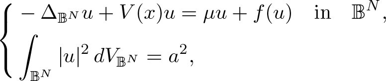
 \begin{equation}
\left\{
\begin{aligned}
&-\Delta_{\mathbb{B}^N} u+A(\epsilon g(x))u=\mu u+f(u) \quad \hbox{in} \quad \mathbb{B}^N,\\
&\int_{\mathbb{B}^N}|u|^2dV_{{\mathbb{B}^N}}=a^2,
\end{aligned}
\right.
\end{equation}
and
 \begin{equation}
\left\{
\begin{aligned}
&-\Delta_{\mathbb{B}^N} u+\tilde{A}(x)u=\mu u+f(u) \quad \hbox{in} \quad \mathbb{B}^N,\\
&\int_{\mathbb{B}^N}|u|^2dV_{{\mathbb{B}^N}}=a^2.
\end{aligned}
\right.
\end{equation}
As the counterparts of Theorems 1.1 and 1.2, we shall prove the following results.
Theorem 1.3. Suppose (g) and  $(A_1)-(A_2)$. If
 $(F_1)$ and
 $(F_2)$ hold, then there are constants
 $\epsilon_* \gt 0$ and
 $a_* \gt 0$ such that, for all
 $\epsilon\in(0,\epsilon_*)$ and
 $a \gt a_*$, Problem (1.8) has a couple of solution
 $(u_a, \mu_a)
\in H^{1}(\mathbb{B}^N)\times \mathbb{R}$, where
 $u_a(x) \gt 0$ for all
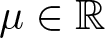
 $x \in \mathbb{B}^N$ and
 $\mu_a \lt 0$.
Theorem 1.4. Suppose (g) and  $(A_1)-(A_2)$. If
 $(F_3)$ holds with
 $p \in(2+\frac{4}{N},2^*)$, then there exist three constants
 $\bar{\epsilon}_* \gt 0$,
 $\bar{a}_* \gt 0$ and
 $\bar{\beta}_*$ such that, for all
 $\epsilon\in(0,\bar{\epsilon}_*)$,
 $a \gt \bar{a}_*$ and
 $\beta\in(0,\bar{\beta}_*)$, Problem (1.8) has a couple of solution
 $(\bar{u}_a, \bar{\mu}_a)
\in H^{1}(\mathbb{B}^N)\times \mathbb{R}$, where
 $\bar{u}_a(x) \gt 0$ for all
 $x \in \mathbb{B}^N$ and
 $\bar{\mu}_a \lt 0$.
Theorem 1.5. Suppose  $(\tilde{A}_1)-(\tilde{A}_2)$. If
 $(F_1)$ and
 $(F_2)$ hold, then there exists a constant
 $\hat{a}^* \gt 0$ such that, for all
 $a \gt \hat{a}^*$, Problem (1.9) admits a couple of solution
 $(\hat{u}_a,\hat{\mu}_a)
\in H^{1}(\mathbb{B}^N)\times \mathbb{R}$, where
 $\hat{u}_a(x) \gt 0$ for all
 $x \in \mathbb{B}^N$ and
 $\hat{\mu}_a \lt 0$.
Theorem 1.6. Suppose  $(\tilde{A}_1)-(\tilde{A}_2)$. If
 $(F_3)$ holds with
 $p \in(2+\frac{4}{N},2^*)$, then there are
 $\tilde{a}^* \gt 0$ and
 $\tilde{\beta}^* \gt 0$ such that, for all
 $a \gt \tilde{a}^*$ and
 $\beta\in (0,\tilde{\beta}^*)$, Problem (1.9) admits a couple of solution
 $(\tilde{u}_a, \tilde{\mu}_a) \in H^{1}(\mathbb{B}^N)\times \mathbb{R}$, where
 $\tilde{u}_a(x) \gt 0$ for all
 $x \in \mathbb{B}^N$ and
 $\tilde{\mu}_a \lt 0$.
Remark 1. We would like to emphasize here that the results in Theorem 1.6 remain true if  $\tilde{A}(x)\equiv0$ for all
 $x\in \mathbb{B}^N$ and the reader would find it eventually in Section 4.1 below.
Remark 2. As pointed out before, we see that Theorems 1.3 and 1.5 are of L 2-subcritical cases and Theorems 1.4 and 1.6 are of L 2-supercritical cases, respectively. It is widely recognized that the constrained minimization approach is an ideal candidate to treat such problems successfully, see e.g. [Reference Jeanjean46, Reference Soave64, Reference Soave65]. Nevertheless, the biggest challenge would occur when we dispose of Theorems 1.4 and 1.6 due to the following facts:
(i) The minimization constant is not well-defined because
$p \gt 2+\frac4N$ in
$(F_3)$;(ii) In the Euclidean space
$\mathbb{R}^N$, it is well-known that if
$u \in L^{2}(\mathbb{R}^N)$, the function
$v_t=t^{{N}/{2}}u(t\cdot)$ preserves the L 2-norm for any t > 0, that is,
$|v_t|_{L^2(\mathbb{R}^N)}=|u|_{L^2(\mathbb{R}^N)}$ for all t > 0. However, this key property does not hold in Hyperbolic space
$\mathbb{B}^N$.


Remark 3. To the best knowledge of us, there seems no similar results in theorems 1.3–1.6 in the literature. In reality, we intend to insist that it is the first time to contemplate the prescribed mass solutions for some nonlinear Schrödinger equations in the Hyperbolic space. On the one hand, because we have the continuous Sobolev embedding  $H^{1}(\mathbb{B}^N) \hookrightarrow L^{p}(\mathbb{B}^N)$ for all
 $p \in [2,2^*]$, the proof of the L 2-subcritical case in Theorems 1.3 and 1.5 is standard to some extent, we shall refer the interested reader to [Reference Alves and Ji4, Reference Alves and Thin7] and their references therein. On the other hand, according to remark 2, the existing arguments, such as those approached in [Reference Bartsch, Molle, Rizzi and Verzini13, Reference Ding and Zhong31, Reference Molle, Riey and Verzini54, Reference Noris, Tavares and Verzini56–Reference Pierotti and Verzini58], are unapplicable to our problems any longer and hence, we must introduce some new subtle techniques and tricks in this article. At this stage, we quote the recent results dealing with some wider classes of L 2-supercritical problems in [Reference Alves and Shen6], but there are at least two unpleasant barriers that prevent us from repeating the procedures directly and simply:
(I) The essential feature of Hyperbolic space, as mentioned in remark 2-(ii), urges us to treat the problems in some new way, see the fundamental hypotheses (g) for example;
(II) In [Reference Alves and Shen6], the sufficiently small mass a > 0 plays a significant role in exploring the existence of normalized solutions, whereas we require the mass a > 0 to be sufficiently large.
Again the results in Theorems 1.1–1.6 are new on the Hyperbolic space  $\mathbb{B}^N$. The striking novelties in Theorems 1.1, 1.3 and 1.4 are twofold: we find a suitable function g that will be disposed to coordinate the Euclidean space
 $\mathbb{R}^N$ and the Hyperbolic space
 $\mathbb{B}^N$ which enables us to treat the problems variationally; On the other hand, the subtle technique which originates from [Reference Alves and Shen6] can be successfully applied to look for normalized solutions of some Schrödinger equations in the Hyperbolic space
 $\mathbb{B}^N$ and we believe that it would be adapted to other non-compact Riemannian domains. Moreover, we show some other technical calculations due to the Laplace–Beltrami operator in the proofs of the main results.
The paper is organized as follows. In Section 2, we introduce some notations and geometric definitions as well as the crucial preliminaries concerning the Hyperbolic space. In Section 3, we shall consider the ground state solutions with different types of the potential. The normalized solutions for L 2-subcritical case and L 2-supercritical case will be handled in Sections 4 and 5, respectively. Finally, in AppendixA, we will show an important compactness embedding that was explored in the present paper.
Notations. From now on in this paper, otherwise mentioned, we use the following notations:
•
$C,C_1,C_2,...$ denote any positive constant, whose value is not relevant.• Let
$(X,\|\cdot\|_X)$ be a Banach space with dual space
$(X^{*},\|\cdot\|_{*})$.• The Palais–Smale sequence at a level
$c\in\mathbb{R}$ corresponding to Φ means that
$\Phi(x_n)\to c$ and
$\Phi^{\prime}(x_n)\to 0$ in
$X^{*}$ as
$n\to\infty$, where
$\{x_n\}\subset X$.•
$|\,\,\,|_p$ denotes the usual norm of the measurable space
$L^{p}(\mathbb{B}^N,dV_{\mathbb{B}^N})$, for all
$p \in [1,+\infty]$.•
$o_{n}(1)$ denotes the real sequences with
$o_{n}(1)\to 0$ as
$n \to +\infty$.• ‘→’ and ‘
$\rightharpoonup$’ stand for the strong and weak convergence in the related function spaces, respectively.


2. Preliminaries
In this section, we shall introduce some notations and definitions adopted in this paper and also recall some embedding related to the Sobolev space associated with the Hyperbolic space.
Let us denote by  $\mathbb{B}^N$ the disk model of the Hyperbolic space, namely the unit disk equipped with the Riemannian metric
 $g_{\mathbb{B}^N}=\sum\limits_{j=1}^N\left(\frac{2}{1-|x|^2}\right)^{2}dx_j^2$. The associated Hyperbolic volume
 $dV_{{\mathbb{B}^N}}$ is given by
 \begin{equation*}dV_{{\mathbb{B}^N}}=\left(\frac{2}{1-|x|^2}\right)^{N}dx,\end{equation*}
where dx stands for the usual Lebesgue measure on  $\mathbb{R}^N$. The Hyperbolic gradient
 $\nabla_{{\mathbb{B}^N}}$ and the hyperbolic Laplacian
 $\Delta_{\mathbb{B}^N}$ are given by
 \begin{equation*}
\nabla_{{\mathbb{B}^N}}=\left(\frac{1-|x|^2}{2}\right)^{2}\nabla,\quad
\Delta_{\mathbb{B}^N}= \left(\frac{1-|x|^2}{2}\right)^{2}\Delta+(N-2)\frac{1-|x|^2}{2}\langle x, \nabla \rangle.
\end{equation*}
We denote by  $H^{1}(\mathbb{B}^N)$ the completion of
 $C^{\infty}_{0}(\mathbb{B}^N)$ under the norm
 \begin{equation*}
\|u\|_{1,2}= \left(\int_{\mathbb{B}^N}(|\nabla_{\mathbb{B}^N}u|_{\mathbb{B}^N}^{2}+|u|^2)\,dV_{{\mathbb{B}^N}}\right)^{\frac{1}{2}},
\end{equation*}
where  $|\nabla_{\mathbb{B}^N}u|_{\mathbb{B}^N}=\sqrt{\langle \nabla_{\mathbb{B}^N}u,\nabla_{\mathbb{B}^N}u\rangle_{\mathbb{B}^N}}$, see e.g. Hebey [Reference Hebey43].
Actually, it can be calculated that the bottom of the spectrum of  $-\Delta_{\mathbb{B}^N}$ on
 $\mathbb{B}^N$ is
 \begin{equation}
\frac{(N-1)^2}4=\inf_{u\in H^1(\mathbb{B}^N)\setminus\{0\}}
\frac{\int_{\mathbb{B}^N}|\nabla_{\mathbb{B}^N}u|_{\mathbb{B}^N}^2\mathrm{d}V_{\mathbb{B}^N}}{\int_{\mathbb{B}^N}|u|^2\mathrm{d}V_{\mathbb{B}^N}}.
\end{equation}
From this,
 \begin{equation*}
\|u\|_{H^{1}(\mathbb{B}^N)}=\left(\int_{\mathbb{B}^N}|\nabla_{\mathbb{B}^N}u|_{\mathbb{B}^N}^{2}\,dV_{{\mathbb{B}^N}}\right)^{\frac{1}{2}},
\end{equation*}
is an equivalent norm to  $\|\;\;\;\|_{1,2}$ in
 $H^{1}(\mathbb{B}^N)$.
Owing to the celebrated Poincaré–Sobolev inequality developed in [Reference Mancini and Sandeep53]: For the dimension  $N \geq 3$ and
 $p \in (2,2^*]$, there is an optimal constant
 $S_{N,p} \gt 0$ such that
 \begin{equation}
S_{N,p}\left(\int_{\mathbb{B}^N}|u|^{p}\,dV_{{\mathbb{B}^N}}\right)^{\frac{2}{p}}\leq \int_{\mathbb{B}^N}\left[|\nabla_{\mathbb{B}^N}u|_{\mathbb{B}^N}^{2}-\frac{(N-1)^2}{4}|u|^2\right]\,dV_{{\mathbb{B}^N}}, \quad \forall u \in H^{1}(\mathbb{B}^N).
\end{equation}
If N = 2, the above inequality is allowed for all p > 2.
The direct consequence of (2.1) is that if the constant  $\lambda \lt \frac{(N-1)^2}4$, then
 \begin{equation*}
\|u\|_{\lambda}=\left(\int_{\mathbb{B}^N}(|\nabla_{\mathbb{B}^N}u|_{\mathbb{B}^N}^{2}-\lambda |u|^2)dV_{{\mathbb{B}^N}}\right)^{\frac{1}{2}},
\quad \forall u \in H^{1}(\mathbb{B}^N),
\end{equation*}
is a norm which is equivalent to the  $\|u\|_{H^{1}(\mathbb{B}^N)}$ on
 $H^{1}(\mathbb{B}^N)$. From now on until the end of the paper, when there is no misunderstanding, we shall adopt the notation
 $\|\cdot\|$ to denote
 $\|\cdot\|_{H^{1}(\mathbb{B}^N)}$ and
 $\|\cdot\|_0$ for short.
The Hyperbolic distance in  $\mathbb{B}^N$. We recall from [Reference Ratcliffe60] that the Hyperbolic distance between
 $x, y\in \mathbb{B}^N$ is given by
 \begin{equation*}
d(x,y)=\cosh^{-1}\left(1+\frac{2|x-y|^2}{(1-|x|^2)(1-|y|^2)}\right),
\end{equation*}
and so a straight computation gives that
 \begin{equation}
d(x,0)=\log\left(\frac{1+|x|}{1-|x|}\right).
\end{equation}
Let us define the Hyperbolic sphere of  $\mathbb{B}^N$ with centre z and radius r > 0 as the set
 \begin{equation*}
S_{\mathbb{B}^N}(z,r)=\big\{x\in\mathbb{B}^N: d(x,z)=r\big\}.
\end{equation*}
It can show that a subset S of  $\mathbb{B}^N$ is a Hyperbolic sphere in
 $\mathbb{B}^N$ if and only if S is a Euclidean sphere in
 $\mathbb{R}^N$ and contained in
 $\mathbb{B}^N$, probably with a different centre and different radius, which can be computed.
We next introduce some information on the isometries of  $\mathbb{B}^N$. Below, we recall the definition of a special type of isometry, namely the Hyperbolic translation. As to the detailed background on the isometry group
 $\mathcal{I}(\mathbb{B}^N)$ of
 $\mathbb{B}^N$, we refer the interested reader to [Reference Ratcliffe60].
Hyperbolic Translation. For  $b=(b_1,b_2,\cdots,b_n)\in\mathbb{B}^N$, define
 \begin{equation*}
\tau_b(x)\triangleq\frac{(1-|b|^2)x+(|x|^2+2x\cdot b+1)b}{|b|^2|x|^2+2x\cdot b+1},\quad x=(x_1,x_2,\cdots,x_n)\in\mathbb{B}^N,
\end{equation*}
then  $\tau_b \in \mathcal{I}(\mathbb{B}^N)$ with
 $\tau_b(0)=b$, where
 $x\cdot b=\sum\limits_{j=1}^Nx_jb_j$. The map τb is called by the Hyperbolic translation of
 $\mathbb{B}^N$ by b.
Definition 2.1. For r > 0, let  $S_r:=\{x\in\mathbb{R}^N:|x|^2=1+r^2\}$ and for
 $z\in S_r$ define
 \begin{equation*}
A(z,r)=B(z,r)\cap\mathbb{B}^N
\end{equation*}
where  $B(z,r)$ is the open ball in the Euclidean space with centre z and radius r > 0.
Using the definition above, we have the following lemma.
Lemma 2.1. See [Reference Bhakta and Sandeep18]
Let  $r_i \gt 0$,
 $z_i \in S_{r_i}$, and
 $A(z_i,r_i)$ be defined as in the above definition for
 $i=1,2$, then there exists an isometry
 $\tau\in \mathcal{I}(\mathbb{B}^N)$ such that
 $\tau(A(z_1,r_1))=A(z_2,r_2)$.
3. Ground state solution
In this section, we mainly deal with the existence of ground state solutions for the nonlinear Schrödinger equation in the Hyperbolic space. More precisely, we shall study Problem (1.5) by three subsections.
3.1. The autonomous problem
In this subsection, we consider the ground state solutions for the following problem
 \begin{equation}
\left\{
\begin{aligned}
&-\Delta_{\mathbb{B}^N} u-\lambda u=f(u) \quad \hbox{in } \quad \mathbb{B}^N,\\
&u(x) \gt 0 \quad \mbox{in} \quad \mathbb{B}^N,
\end{aligned}
\right.
\end{equation}
where  $\lambda \lt \frac{(N-1)^2}4$ is a constant. We recall that a weak solution
 $u\in H^{1}(\mathbb{B}^N)$ to Problem (3.1) corresponds to a critical point of the functional
 $I:H^{1}(\mathbb{B}^N) \to \mathbb{R}$ given by
 \begin{equation}
I(u)=\frac{1}{2}\int_{\mathbb{B}^N}(|\nabla_{\mathbb{B}^N} u|_{\mathbb{B}^N}^2-\lambda |u|^2) \,dV_{{\mathbb{B}^N}}
-\int_{\mathbb{B}^N}F(u)\,dV_{{\mathbb{B}^N}},\,\, u\in H^{1}(\mathbb{B}^N).
\end{equation}
Moreover, similar to [Reference Willem69],  $I \in {C}^{1}(H^{1}(\mathbb{B}^N),\mathbb{R})$ with
 \begin{equation*}
I'(u)v=\int_{\mathbb{B}^N}\big(\langle \nabla_{\mathbb{B}^N} u, \nabla_{{\mathbb{B}^N}}v\rangle_{{\mathbb{B}^N}}
-\lambda uv\big)\,dV_{{\mathbb{B}^N}}
-\int_{\mathbb{B}^N}f(u)v\,dV_{{\mathbb{B}^N}}, \quad \forall u,v \in H^{1}(\mathbb{B}^N).
\end{equation*}
Associated with the functional I, we have the Nehari manifold, which is defined by
 \begin{equation*}
\mathcal{N}=\{u \in H^{1}(\mathbb{B}^N) \setminus \{0\}\,:\, I'(u)u=0\},
\end{equation*}
and the minimization problem
 \begin{equation}
d=\inf_{u \in \mathcal{N}}I(u).
\end{equation}
Since we intend to find a positive solution and the nonlinearity f is odd by  $(f_1)$, hereafter we are assuming that
 $f(t)=0$ for all
 $t \leq 0$. Moreover, for simplicity, we let
 $\lambda=-1$ in Problem (3.1).
Our main result concerning the autonomous Problem (3.1) is the following:
Theorem 3.1. If  $(f_1)-(f_4)$ hold, then Problem (3.1) admits a ground state solution.
The proof of the above theorem will be divided into several lemmas.
Lemma 3.2. Assume  $(f_1)-(f_4)$ are satisfied, then the following conclusions are true:
(i) Given a
$u\in H^1(\mathbb{B}^N)\setminus \{0\}$, there exists a unique
$t_u \gt 0$ such that
$m(u)\triangleq t_uu\in \mathcal{N}$ and
$I\left(m(u)\right)=\max I\left(\mathbb{R}^+u\right)$.(ii) There exists
$\beta_0 \gt 0$ such that
$\|u\|\geq\beta_0$ for all
$u\in\mathcal{N}$.(iii) I is bounded from below on
$\mathcal{N}$ by a positive constant.(iv) I is coercive on
$\mathcal{N}$, i.e.,
$I(u)\to\infty$ as
$\|u\|\to\infty,u\in\mathcal{N}$.(v) Suppose
$\mathcal{V}\subset H^1(\mathbb{B}^N)\setminus\{0\}$ is a compact subset, then there is an
$\mathcal{R} \gt 0$ such that
$I\leq0$ on
$\mathbb{R}^{+}\mathcal{V}\setminus \{u\in H^1(\mathbb{B}^N)\setminus \{0\}:\|u\|\leq \mathcal{R}\}$.


Proof. The proof is standard by now, and we refer the reader to [Reference Szulkin and Weth66, Reference Szulkin and Weth67] for the details.
Then, we consider the unit sphere  $\mathbb{S}\triangleq\{u\in H^1(\mathbb{B}^N): \|u\|= 1\}$ of
 $H^1(\mathbb{B}^N)$ and the mapping
 $\mathbb{S}\to \mathcal{N}$,
 $u\mapsto m(u)$. Motivated by [Reference Szulkin and Weth66, lemma 2.8], owing to Lemma 3.2, we have the following key observations: the mapping m is continuous and moreover m is homeomorphism between
 $\mathbb{S}$ and
 $\mathcal{N}$, where the inverse of m is given by
 \begin{equation*}
m^{-1}(u)=\frac u{\|u\|}.
\end{equation*}
Now, we study the functional  $\Phi:\mathbb{S}\to\mathbb{R}$ which defined by
 \begin{equation*}
\Phi(w)\triangleq I(m(w)).
\end{equation*}
Proceeding as [Reference Szulkin and Weth66, proposition 2.9 and corollary 2.10], by exploiting Lemma 3.2 and the above observations, it permits us to derive the following lemma whose detailed proof will be omitted.
Lemma 3.3. Assume  $(f_1)-(f_4)$ are satisfied, then we have
(i)
$\Phi\in \mathcal{C}^1(\mathbb{S},\mathbb{R})$ and
\begin{equation*}
\Phi^\prime(w)z=\|m(w)\| I^\prime(m(w)) z, ~\forall z\,{\in}\, T_w\mathbb{S}\triangleq
\left\{\!v\in H^1(\mathbb{B}^N)\,{:}\,\int_{\mathbb{B}^N} v wdV_{\mathbb{B}^N}=0\!\right\}\!.
\end{equation*}(ii)
$(w_n)$ is a Palais–Smale sequence for Φ if and only if
$(m(w_n))$ is a Palais–Smale sequence for I.(iii)
$w\in \mathbb{S}$ is a critical point of Φ if and only if
$m(w)\in\mathcal{N}$ is a critical point of I. Moreover, the corresponding critical values of Φ and I coincide and
$\inf_{\mathbb{S}}\Phi=\inf_{\mathcal{N}}I$.


According to lemmas 3.2 and 3.3, we are able to show that there is a Palais–Smale sequence for I at the level d > 0, where d comes from (3.3). With such a sequence  $\{u_n\}\subset H^1(\mathbb{B}^N)$, say it
 $(PS)_d$, we will show that it contains a strongly convergent subsequence in
 $H^1(\mathbb{B}^N)$. Before proceeding with it, we are going to introduce the following result.
Lemma 3.4. Assume  $(f_1)-(f_4)$ are satisfied and let
 $\{u_n\}\subset H^{1}(\mathbb{B}^N)$ be a
 $(PS)_c$ sequence for I. If
 $\tau_n \in \mathcal{I}(\mathbb{B}^N)$ and
 $\tilde{u}_n=u_n \circ \tau_n$, then
 $\{\tilde{u}_n\}$ is also a
 $(PS)_c$ sequence for I.
Proof. Since the functional I is invariant under isometries in  $\mathcal{I}(\mathbb{B}^N)$, the proof is standard and we refer to [Reference Bhakta and Sandeep18, lemma 3.2].
Our next result is a compactness theorem on the Nehari manifold  $\mathcal{N}$, and it is a useful tool in the study of the autonomous cases as well as non-autonomous cases.
Theorem 3.5. (Compactness theorem on  $\mathcal{N}$) Assume
 $(f_1)-(f_4)$ are satisfied and let
 $(u_n)\subset \mathcal{N} $ be a sequence satisfying
 $I(u_n) \to d$. Then, for some subsequence either
 $\text{i)}$
 $(u_n)$ is strongly convergent,
or
 $\text{ii)}$ there exists
 $(\tau_n) \subset \mathcal{I}(\mathbb{B}^N)$ such that the sequence
 $\tilde{u}_n=u_n \circ \tau_n$ is strongly convergent to a function
 $\tilde{u}\in \mathcal{N}$ with
 $I(\tilde{u})=d$.
Proof. First of all, by using Ekeland’s variational principle and Lemma 3.3, we can assume that  $\{u_n\}$ is a
 $(PS)_d$ sequence for I. Moreover,
 $\{u_n\}$ is bounded by Lemma 3.2-(iv), then we shall further assume that for some subsequence, still denoted by itself,
 $ u_n \rightharpoonup u$ in
 $H^{1}(\mathbb{B}^N)$ for some
 $u \in H^{1}(\mathbb{B}^N)$. Exploiting Lemma 3.2-(iii), there holds d > 0, it then follows that
 \begin{equation*}
\liminf_{n \to +\infty}\int_{\mathbb{B}^N}|u_n|^{q}\,dV_{\mathbb{B}^N}=\delta' \gt 0,
\end{equation*}
because
 \begin{equation*}
\liminf_{n \to +\infty}\int_{\mathbb{B}^N}F(u_n)\,dV_{{\mathbb{B}^N}} \gt 0
\end{equation*}
and  $\{u_n\}$ is bounded in
 $L^{2}(\mathbb{B}^N)$. In what follows, we will divide our analysis into two cases:
Case 1:  ${u} \not=0$.
In light of  $\{u_n\}$ is a
 $(PS)_d$ sequence, we immediately conclude that
 $I'(u)=0$, and so,
 $u \in \mathcal{N}$. Thereby, it can be derived from Fatou’s lemma and
 $(f_4)$ that
 \begin{equation*}
d \leq I(u)=I(u)-\frac{1}{2}I'(u)u \leq \lim_{n\to +\infty}(I(u_n)-\frac{1}{2}I'(u_n)u_n)=\lim_{n\to +\infty}I(u_n)=d,
\end{equation*}
showing that  $I(u)=d$. This fact, jointly with
 $\{u_n\}$ is a
 $(PS)_d$ sequence, does imply that
 \begin{equation*}\begin{gathered}
\left(\frac{1}{2}-\frac{1}{\theta}\right)\|u_n\|^2+\int_{\mathbb{B}^N}\left(\frac{1}{\theta}f(u_n)u_n
-F(u_n)\right)\,dV_{{\mathbb{B}^N}}\hfill\\
\ \ \ \ =\left(\frac{1}{2}-\frac{1}{\theta}\right)\|u\|^2+\int_{\mathbb{B}^N}
\left(\frac{1}{\theta}f(u)u-F(u)\right)\,dV_{{\mathbb{B}^N}}+o_n(1),\hfill\\
\end{gathered}
\end{equation*}
from where it yields that  $u_n \to u$ in
 $H^{1}(\mathbb{B}^N)$. So, the proof is done.
Case 2: u = 0.
Arguing as the proof of [Reference Bhakta and Sandeep18, theorem 3.3], there are  $\tau_n \in \mathcal{I}(\mathbb{B}^N$),
 $x_0 \in S_{\sqrt{3}}$ and
 $0 \lt \delta \lt S_{N,q}$ of such way that the sequence
 $\tilde{u}_n=u_n \circ \tau_{b_n}$ satisfies
 \begin{equation*}
\int_{A(x_0,\sqrt{3})}|\tilde{u}_n|^{q}\,dV_{{\mathbb{B}^N}}=\sup_{x \in S_{\sqrt{3}}}\int_{A(x,\sqrt{3})}|u_n|^{q}\,dV_{{\mathbb{B}^N}}=\delta.
\end{equation*}
Furthermore,  $\{\tilde{u}_n\}$ is also a
 $(PS)_d$ for I by Lemma 3.4. Using Lemma 3.2-(iv) again, for some subsequence, still denoted by
 $\{\tilde{u}_n\}$, there exists a
 $\tilde{u}\in H^{1}(\mathbb{B}^N)$ such that
 $\tilde{u}_n \rightharpoonup \tilde{u}$ in
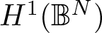 $H^{1}(\mathbb{B}^N)$.
Claim 3.6.  $\tilde{u} \not= 0$.
Otherwise, we could suppose that  $\tilde{u}=0$. Since
 $\{\tilde{u}_n\}$ is a
 $(PS)_d$ sequence for I, owing to the proof of [Reference Bhakta and Sandeep18, theorem 3.3] again, we use Lemma 2.1 to prove that
 \begin{equation}
\int_{\mathbb{B}^N \cap [|x| \geq r]}|\tilde{u}_n|^q\,dV_{{\mathbb{B}^N}} \to 0,
\end{equation}
for all  $r \in (2-\sqrt{3},1)$. Recalling that the embedding
 $H^{1}(\mathbb{B}^N) \hookrightarrow L^{q}(\mathbb{B}^N \cap [|x| \lt r],dV_{{\mathbb{B}^N}})$ is compact, see Lemma A.1 in the Appendix, we have that
 \begin{equation}
\int_{\mathbb{B}^N \cap [|x| \lt r]}|\tilde{u}_n|^q\,dV_{{\mathbb{B}^N}} \to 0.
\end{equation}
 \begin{equation*}
\int_{\mathbb{B}^N}|\tilde{u}_n|^q\,dV_{{\mathbb{B}^N}} \to 0,
\end{equation*}
which contradicts with the limit below
 \begin{equation*}
\liminf_{n \to +\infty}\int_{\mathbb{B}^N}|\tilde{u}_n|^{q}\,dV_{{\mathbb{B}^N}}=\liminf_{n \to +\infty}\int_{\mathbb{B}^N}|u_n|^{q}\,dV_{{\mathbb{B}^N}}=\delta' \gt 0,
\end{equation*}
showing the claim 3.6. In the same spirit of Case 1, we see that  $\tilde{u}_n \to \tilde{u}$ along a subsequence in
 $H^{1}(\mathbb{B}^N)$. This proves the theorem.
Proof of Theorem 3.1
As an immediate consequence of the compactness theorem exhibited in Theorem 3.5, we can prove that Problem (3.1) has a ground state solution  $u\in H^1(\mathbb{B}^N)$. To finish the proof, we will prove that
 $u(x) \gt 0$ for all
 $x\in \mathbb{B}^N$.
From the definition of the variational functional I, one can check that  $I(|u|)=I(u)=d$ and
 $|u|\in \mathcal{N}$ which permit us to replace u with
 $|u|$. In order to prove that
 $u(x) \gt 0$ for all
 $x \in \mathbb{B}^N$, it is enough to apply the celebrated Harnack inequality (see e.g. [Reference Gilbarg and Trudinger38, theorem 8.20]). Indeed, by considering the functions
 \begin{equation*}
p(x)=\left(\frac{2}{1-|x|^2}\right)^{2} \quad \mbox{and} \quad v(x)=p^{\frac{N-2}{4}}(x)u(x), \quad x \in \mathbb{B}^N,
\end{equation*}
a direct computation implies that v is a solution of the Euclidean type problem
 \begin{equation*}
\left\{
\begin{array}{l}
-\Delta v= p^{\frac{N+2}{4}}\left(f(p(x)^{\frac{2-N}{4}}v)+ \hat{\lambda}p(x)^{\frac{2-N}{4}}v\right), \quad \mbox{in} \quad \mathbb{B}^N
, \\
v=0, \quad \mbox{on} \quad \partial \mathbb{B}^N,
\end{array}
\right.
\end{equation*}
where  $\hat{\lambda}=\lambda-\frac{N(N-2)}{4}$ and
 $\mathbb{B}^N$ is endowed with Euclidean metric.
Assume by contradiction that there exists  $x_0 \in \mathbb{B}^N$ such that
 $v(x_0)=0$. Since
 $v \not=0$, there exists
 $x_1 \in \mathbb{B}^N$ such that
 $v(x_1) \gt 0$. Have this in mind, fix
 $0 \lt R \lt 1$ such that
 $x_0,x_1 \in B_R(0)$. By means of [Reference Gilbarg and Trudinger38, theorem 8.20], there exists a constant C > 0 such that
 \begin{equation*}
\sup_{y \in B_R(0)}v(y) \leq C\inf_{y \in B_R(0)}v(y),
\end{equation*}
which is absurd, because in this case
 \begin{equation*}
\sup_{y \in B_R(0)}v(y) \gt 0 \quad \mbox{and} \quad \inf_{y \in B_R(0)}v(y)=0.
\end{equation*}
This completes the proof.
3.2. The potential is an asymptotical constant
In this subsection, our goal is to explore a ground state solution for the following problem
 \begin{equation}
\left\{
\begin{aligned}
&-\Delta_{\mathbb{B}^N} u+\tilde{A}(x)u=f(u) \quad \hbox{in } \quad \mathbb{B}^N,\\
&u(x) \gt 0 \quad \mbox{in} \quad \mathbb{B}^N,
\end{aligned}
\right.
\end{equation}
where the potential  $\tilde{A}:\mathbb{B}^N\to\mathbb{R}$ satisfies the conditions
 $(\tilde{A}_1)$ and
 $(\tilde{A}_2)$.
Therefore, the main result involving the non-autonomous Problem (3.6) is the following:
Theorem 3.7. Assume  $(f_1)-(f_4)$ and
 $(\tilde{A}_1)-(\tilde{A}_2)$. Then, Problem (3.6) has a ground state solution.
Proceeding as before, to look for weak solutions for Problem (3.6), we consider the existence of critical points of the functional  $J:H^{1}(\mathbb{B}^N) \to \mathbb{R}$ given by
 \begin{equation}
J(u)=\frac{1}{2}\int_{\mathbb{B}^N}(|\nabla_{\mathbb{B}^N} u|_{\mathbb{B}^N}^2+\tilde{A}(x)|u|^2) \,dV_{{\mathbb{B}^N}}
-\int_{\mathbb{B}^N}F(u)\,dV_{{\mathbb{B}^N}},\,\, u\in H^{1}(\mathbb{B}^N).
\end{equation}
Moreover, similar to [Reference Willem69] again,  $J \in {C}^{1}(H^{1}(\mathbb{B}^N),\mathbb{R})$ with
 \begin{equation*}
J'(u)v=\int_{\mathbb{B}^N}\big(\langle\nabla_{\mathbb{B}^N} u, \nabla_{{\mathbb{B}^N}}v\rangle_{\mathbb{B}^N}+\tilde{A}(x)uv\big)\,dV_{{\mathbb{B}^N}}
-\int_{\mathbb{B}^N}f(u)v\,dV_{{\mathbb{B}^N}}, \quad \forall u,v \in H^{1}(\mathbb{B}^N).
\end{equation*}
Associated with J, we have the Nehari manifold given by
 \begin{equation*}
\mathcal{M}=\{u \in H^{1}(\mathbb{B}^N) \setminus \{0\}\,:\, J'(u)u=0\},
\end{equation*}
and define the minimization problem
 \begin{equation}
\tilde{d}=\inf_{u \in \mathcal{M}}J(u).
\end{equation}
To overcome the lack of compactness, we will deal with the ‘limit problem’ with respect to Problem (3.6). We denote the variational functional by  $J_\infty:H^{1}(\mathbb{B}^N) \to \mathbb{R}$ given by
 \begin{equation}
J_\infty(u)=\frac{1}{2}\int_{\mathbb{B}^N}(|\nabla_{\mathbb{B}^N} u|_{\mathbb{B}^N}^2+\tilde{A}_\infty|u|^2) \,dV_{{\mathbb{B}^N}}
-\int_{\mathbb{B}^N}F(u)\,dV_{{\mathbb{B}^N}},\,\, u\in H^{1}(\mathbb{B}^N).
\end{equation}
Similarly,  $J_\infty \in C^{1}(H^{1}(\mathbb{B}^N),\mathbb{R})$ with
 \begin{equation*}
J_\infty'(u)v=\int_{\mathbb{B}^N}(\langle\nabla_{\mathbb{B}^N} u, \nabla_{{\mathbb{B}^N}}v\rangle_{\mathbb{B}^N}+\tilde{A}_\infty uv)\,dV_{{\mathbb{B}^N}}
-\int_{\mathbb{B}^N}f(u)v\,dV_{{\mathbb{B}^N}}, \quad \forall u,v \in H^{1}(\mathbb{B}^N).
\end{equation*}
Associated with  $J_\infty$, we also introduce the Nehari manifold given by
 \begin{equation*}
\mathcal{M_\infty}=\{u \in H^{1}(\mathbb{B}^N) \setminus \{0\}\,:\, J_\infty'(u)u=0\},
\end{equation*}
and the minimization problem
 \begin{equation}
\tilde{d}_\infty=\inf_{u \in \mathcal{M}_\infty}J_\infty(u).
\end{equation}
By definitions of  $\tilde{d}$ and
 $\tilde{d}_\infty$ in (3.8) and (3.10), adopting
 $(\tilde{A}_2)$, it is easy to check that
 \begin{equation}
\tilde{d} \lt \tilde{d}_\infty.
\end{equation}
Let us recall the discussions in Section 3.1, we can conclude that the conclusions proved in lemmas 3.2 and 3.3 remain true for the variational functions J and  $J_\infty$. Thus, without loss of generality, we will exploit them directly in this subsection.
Suppose that  $\{u_n\}\subset H^1(\mathbb{B}^N)$ is a bounded
 $(PS)_{\tilde{d}}$ sequence of J, passing to a subsequence if necessary, there exists a function
 $u\in H^1(\mathbb{B}^N)$ such that
 $u_n\rightharpoonup u$ in
 $H^1(B^N)$. Thanks to
 $(\tilde{A}_2)$, we can prove that the weak limit u is nontrivial.
Lemma 3.8. Assume  $(f_1)-(f_4)$ and
 $(\tilde{A}_1)-(\tilde{A}_2)$, the weak limit u is nontrivial, that is,
 $u \not=0$.
Proof. Assume by contradiction that u = 0 and let  $t_n \gt 0$ such that
 $t_nu_n \in \mathcal{M}_\infty$. The standard calculations show that
 $\{t_n\}$ is bounded, and so,
 \begin{align*}
\tilde{d } +o_n(1)&=J(u_n)= \max_{t \geq 0}J(tu_n) \geq J(t_nu_n)=J_\infty(t_nu_n)
+\frac{t_n^2}{2}\int_{\mathbb{B}^N}(\tilde{A}(x)-\tilde{A}_\infty)\\ &\quad\times |u_n|^2\,dV_{{\mathbb{B}^N}},
\end{align*}
where we have used a similar property in Lemma 3.2-(i) in the second equality. From this,
 \begin{equation*}
\tilde{d} +o_n(1) \geq \tilde{d}_\infty + \frac{t_n^2}{2}\int_{\mathbb{B}^N}(\tilde{A}(x)-\tilde{A}_\infty)|u_n|^2\,dV_{{\mathbb{B}^N}}.
\end{equation*}
In light of the fact that  $\{t_n\}$ is bounded, then the proof is done if we can verify that
 \begin{equation}
\int_{\mathbb{B}^N}(\tilde{A}(x)-\tilde{A}_\infty)|u_n|^2dV_{{\mathbb{B}^N}} \to 0
\end{equation}
loading to
 \begin{equation*}
\tilde{d} \geq \tilde{d}_\infty,
\end{equation*}
which contradicts with (3.11). Now, we focus on showing the validity of (3.12).
Owing to (2.3), one sees that  $\tilde{A}(x)\to \tilde{A}_\infty$ as
 $d(x,0)\to\infty$ for all
 $x\in \mathbb{B}^N$ by
 $(\tilde{A}_2)$. Therefore, given a ɛ > 0, there is an
 $\tilde{r}\in(0,1)$ such that
 $|\tilde{A}(x)-\tilde{A}_\infty| \lt \varepsilon$ for all
 $\tilde{r} \lt |x| \lt 1$ and so
 \begin{equation*}
\int_{\mathbb{B}^N\cap[\tilde{r} \lt |x| \lt 1]}|\tilde{A}(x)-\tilde{A}_\infty||u_n|^2dV_{{\mathbb{B}^N}}\leq C \varepsilon,
\end{equation*}
where C > 0 is independent of  $n\in \mathbb{N}$. Consider the embedding
 $H^{1}(\mathbb{B}^N) \hookrightarrow L^{2}(\mathbb{B}^N \cap [|x|\leq\tilde{r}])$ is compact, see Lemma A.1 in the Appendix one has that
 \begin{equation*}
\int_{\mathbb{B}^N\cap[|x|\leq\tilde{r}]]}|\tilde{A}(x)-\tilde{A}_\infty||u_n|^2dV_{{\mathbb{B}^N}}\leq C_{\tilde{r}}
\int_{\mathbb{B}^N\cap[|x|\leq\tilde{r}]]}|u_n|^2dV_{{\mathbb{B}^N}}=o_n(1),
\end{equation*}
where  $C_{\tilde{r}} \gt 0$ is independent of
 $n\in \mathbb{N}$. Letting
 $n\to\infty$ and then
 $\varepsilon\to0^+$, we finish the proof of this lemma.
Proof Theorem 3.7
With Lemma 3.8 in hand, we know that u is a nontrivial critical point for J, and so,  $J(u) \geq \tilde{d}$. On the other hand, one has
 \begin{equation*}
J(u)=J(u)-\frac{1}{2}J'(u)u=\frac{1}{2}\int_{\mathbb{B}^N}(f(u)u-2F(u))dV_{{\mathbb{B}^N}}.
\end{equation*}
By Fatou’s lemma,
 \begin{align*}
\frac{1}{2}\int_{\mathbb{B}^N}(f(u)u-2F(u))dV_{{\mathbb{B}^N}} &\leq \liminf_{n \to +\infty}\frac{1}{2}\int_{\mathbb{B}^N}(f(u_n)u_n-2F(u_u))dV_{{\mathbb{B}^N}}\\ &=\liminf_{n \to +\infty}J(u_n)=\tilde{d},
\end{align*}
from where it concludes  $J(u)=\tilde{d}$, showing that u is indeed a nontrivial ground state solution of Problem (3.6). Concerning the positivity of u, the reader can refer to the proof of Theorem 3.1, we omit it here. The proof is completed.
3.3. Rabinbowitz’s type potential
In this subsection, we will study the existence of ground state solution for the following class of problem
 \begin{equation}
\left\{
\begin{aligned}
&-\Delta_{\mathbb{B}^N} u+A(\epsilon g(x))u=f(u) \quad \hbox{in } \quad \mathbb{B}^N,\\
&u(x) \gt 0 \quad \mbox{in} \quad \mathbb{B}^N,
\end{aligned}
\right.
\end{equation}
where ϵ > 0 denotes a positive parameter,  $g:\mathbb{B}^N \to \mathbb{R}^N$ is a continuous and surjective function satisfying the condition (g), while
 $A:\mathbb{R}^N \to \mathbb{R}$ is a continuous function satisfying
 $(A_1)$ and
 $(A_2)$. As mentioned in the introduction, we are assuming that
 $A(0)=\displaystyle \inf_{x \in \mathbb{B}^N}A(x)$.
Our main result involving Rabinowitz-type potential is the following:
Theorem 3.9. Assume  $(f_1)-(f_4)$, (g) and
 $(A_3)-(A_4)$. Then, there exists a sufficiently small
 $\epsilon_0 \gt 0$ such that Problem (3.13) admits a ground state solution for all
 $\epsilon\in(0,\epsilon_0)$.
Again to deal with Theorem 3.9, we look for the critical points for the variational functional  $I_\epsilon:H^{1}(\mathbb{B}^N) \to \mathbb{R}$ given by
 \begin{align}
I_\epsilon(u)=\frac{1}{2}\int_{\mathbb{B}^N}\big(|\nabla_{\mathbb{B}^N} u|^2_{\mathbb{B}^N}+A(\epsilon g(x))|u|^2\big) dV_{{\mathbb{B}^N}}
-\int_{\mathbb{B}^N}F(u)\,dV_{{\mathbb{B}^N}},\quad u\in H^{1}(\mathbb{B}^N).\nonumber\\
\end{align}
Moreover, similar to [Reference Willem69] again,  $I_\epsilon \in C^{1}(H^{1}(\mathbb{B}^N),\mathbb{R})$ with
 \begin{align*}
I_\epsilon'(u)v=\int_{\mathbb{B}^N}\big(\langle\nabla_{\mathbb{B}^N} u, \nabla_{{\mathbb{B}^N}}v\rangle_{\mathbb{B}^N}+A(\epsilon g(x))uv\big)
dV_{{\mathbb{B}^N}}&-\int_{\mathbb{B}^N}f(u)v\,dV_{{\mathbb{B}^N}},\\& \quad \forall u,v \in H^{1}(\mathbb{B}^N).
\end{align*}
Associated with Iϵ, we introduce the Nehari manifold given by
 \begin{equation*}
\mathcal{N}_\epsilon=\{u \in H^{1}(\mathbb{B}^N) \setminus \{0\}\,:\, I_\epsilon'(u)u=0\}
\end{equation*}
and the minimization problem
 \begin{equation}
d_\epsilon=\inf_{u \in \mathcal{N}_\epsilon}I_\epsilon(u).
\end{equation}
Inspired by the handling in Section 3.2, we denote by  $I_0,I_\infty:H^{1}(\mathbb{B}^N) \to \mathbb{R}$ the following variational functionals given by
 \begin{equation}
I_\infty(u)=\frac{1}{2}\int_{\mathbb{B}^N}(|\nabla_{\mathbb{B}^N} u|_{\mathbb{B}^N}^2+A_\infty|u|^2)
dV_{{\mathbb{B}^N}}-\int_{\mathbb{B}^N}F(u)\,dV_{{\mathbb{B}^N}},\,\, u\in H^{1}(\mathbb{B}^N)
\end{equation}
and
 \begin{equation}
I_0(u)=\frac{1}{2}\int_{\mathbb{B}^N}(|\nabla_{\mathbb{B}^N} u|_{\mathbb{B}^N}^2+A_0|u|^2)
dV_{{\mathbb{B}^N}}-\int_{\mathbb{B}^N}F(u)\,dV_{{\mathbb{B}^N}},\,\, u\in H^{1}(\mathbb{B}^N)
\end{equation}
It is simple to find that  $I_0, I_\infty \in C^{1}(H^{1}(\mathbb{B}^N),\mathbb{R})$ with
 \begin{equation*}
\left\{
\begin{array}{l}
\displaystyle I_\infty'(u)v=\int_{\mathbb{B}^N}\big(\langle\nabla_{\mathbb{B}^N} u,
\nabla_{{\mathbb{B}^N}}v\rangle_{\mathbb{B}^N}+A_\infty uv\big)dV_{{\mathbb{B}^N}}
-\int_{\mathbb{B}^N}f(u)v\,dV_{{\mathbb{B}^N}}, \\ \quad \forall u,v \in H^{1}(\mathbb{B}^N),\\
\displaystyle I_0'(u)v=\int_{\mathbb{B}^N}\big(\langle\nabla_{\mathbb{B}^N} u, \nabla_{{\mathbb{B}^N}}v\rangle_{\mathbb{B}^N}+A_0uv\big)
dV_{{\mathbb{B}^N}}
-\int_{\mathbb{B}^N}f(u)v\,dV_{{\mathbb{B}^N}}, \\ \quad \forall u,v \in H^{1}(\mathbb{B}^N)
\end{array}
\right.
\end{equation*}
Associated with the functionals  $I_\infty$ and I 0, we need the Nehari manifolds given by
 \begin{equation*}
\left\{
\begin{array}{ll}
\displaystyle \mathcal{M}_\infty=\{u \in H^{1}(\mathbb{B}^N) \setminus \{0\}: I_\infty'(u)u=0\}, \\
\displaystyle \mathcal{M}_0=\{u \in H^{1}(\mathbb{B}^N) \setminus \{0\}: I_0'(u)u=0\},
\end{array}
\right.
\end{equation*}
and the minimization problems
 \begin{equation}
\left\{
\begin{array}{ll}
\displaystyle d_\infty=\inf_{u \in \mathcal{M}_\infty}I_\infty(u),\\
\displaystyle d_0=\inf_{u \in \mathcal{M}_0}I_0(u).
\end{array}
\right.\end{equation}
According to the definitions of d 0 and  $d_\infty$, by
 $(A_2)$, it is easy to check that
 \begin{equation}
d_0 \lt d_\infty.
\end{equation}
Now, we invite the reader to realize that lemmas 3.2 and 3.3 are still true for the variational functions Iϵ,  $I_\infty$ and I 0 under the assumptions in Theorem 3.9. As a consequence, we continue to adopt their conclusions without detailed proofs.
Therefore, for every fixed ϵ > 0, we can suppose that there exists a bounded  $(PS)_{{d}_\epsilon}$ sequence
 $\{u_n\}\subset H^1(\mathbb{B}^N)$ of Iϵ. So, there is a function
 $u\in H^1(\mathbb{B}^N)$ such that
 $u_n\rightharpoonup u$ along a subsequence in
 $H^1(\mathbb{B}^N)$. Proceeding as the proof of Theorem 3.7, we shall accomplish the proof of Theorem 3.9 by verifying that the weak limit u is nontrivial, namely
 $u\not=0$.
Lemma 3.10. Assume  $(f_1)-(f_4)$, (g) and
 $(A_3)-(A_4)$. Then there holds
 $\displaystyle \lim_{\epsilon \to 0}d_\epsilon=d_0$, and so, there is a sufficiently small
 $\epsilon_0 \gt 0$ such that
 $d_\epsilon \lt d_\infty$ for all
 $\epsilon \in (0, \epsilon_0)$.
Proof. According to the discussions in Theorem 3.1, there is a  $U_0\in H^1(\mathbb{B}^N)$ such that
 \begin{equation*}
I_0(U_0)=d_0 \gt 0 \quad \mbox{and} \quad I'_0(U_0)=0.
\end{equation*}
Let  $t_\epsilon \gt 0$ be such that
 $t_\epsilon U_0 \in \mathcal{N}_\epsilon$. A simple argument shows that
 $\{t_\epsilon\}$ is bounded with respect to ϵ > 0 and so we can assume that
 $t_\epsilon \to t_0$ as
 $\epsilon\to0^+$. Having this in mind, we arrive at
 \begin{equation*}
d_\epsilon \leq I_\epsilon(t_\epsilon U_0)=\frac{t_\epsilon^2}{2}\int_{\mathbb{B}^N}(|\nabla_{\mathbb{B}^N} U_0|^2
+A(\epsilon g(x))|U_0|^2) \,dV_{{\mathbb{B}^N}}-\int_{\mathbb{B}^N}F(t_\epsilon U_0)dV_{{\mathbb{B}^N}}.
\end{equation*}
 \begin{equation*}
\lim_{\epsilon\to0^+}\int_{\mathbb{B}^N}|A(\epsilon g(x))-A(0)||U_0|^2dV_{{\mathbb{B}^N}}=0.
\end{equation*}
Indeed, since  $A \in L^{\infty}(\mathbb{R}^N)$, it follows that
 \begin{equation*}
|A(\epsilon g(x))-A(0)||U_0|^2 \leq 2|A|_\infty |U_0|^2 \in L^{1}(\mathbb{B}^N), \quad \forall \epsilon \gt 0.
\end{equation*}
Now, using the fact that A is a continuous function, Lebesgue’s Dominated Convergence theorem yields that the claim above is true.
Applying again Lebesgue’s Dominated Convergence theorem, we also get
 \begin{equation*}
\lim_{\epsilon \to 0^+}\left(\frac{t_\epsilon^2}{2}\int_{\mathbb{B}^N}(|\nabla_{\mathbb{B}^N} U_0|^2+A(0)|U_0|^2) \,dV_{{\mathbb{B}^N}}
-\int_{\mathbb{B}^N}F(t_\epsilon U_0)\,dV_{{\mathbb{B}^N}} \right)=I_0(t_0U_0),
\end{equation*}
which together with claim 3.11 reveals the inequality below
 \begin{equation}
\limsup_{\epsilon \to 0^+}d_\epsilon \leq I_0(t_0U_0)\leq \max_{t \geq 0}I_0(tU_0)=I_0(U_0)=d_0.
\end{equation}
On the other hand, recalling  $A(0)=\displaystyle \inf_{z \in \mathbb{R}^N}A(z)=A_0$, one finds
 \begin{equation*}
I_0(u) \leq I_\epsilon(u), \quad \forall u \in H^{1}(\mathbb{B}^N),
\end{equation*}
implying that
 \begin{equation*}
d_0 \leq d_\epsilon, \quad \forall \epsilon \gt 0.
\end{equation*}
Thereby,
 \begin{equation}
d_0 \leq \liminf_{\epsilon \to 0} d_\epsilon.
\end{equation}
 \begin{equation*}
\lim_{\epsilon \to 0^+} d_\epsilon=d_0.
\end{equation*}
The limit above combined with (4.30) yields that there exists a  $\epsilon_0 \gt 0$ such that
 $d_\epsilon \lt d_\infty$ for all
 $\epsilon \in (0, \epsilon_0)$. The proof is completed.
Lemma 3.12. Assume  $(f_1)-(f_4)$, (g) and
 $(A_3)-(A_4)$. Then there exists a sufficiently small
 $\epsilon\in(0,\epsilon_0)$ such that the weak limit
 $u\not=0$ for all fixed
 $\epsilon \in (0,\epsilon_0)$.
Proof. Assume by contradiction that u = 0 and let  $t_n \gt 0$ such that
 $t_nu_n \in \mathcal{M}_\infty$. It is easy to prove that
 $\{t_n\}$ is bounded. Since
 $\{u_n\}\subset \mathcal{M}_\epsilon$ is a
 $(PS)_{d_\epsilon}$ sequence of Iϵ, one sees that
 \begin{equation*}
d_\epsilon +o_n(1)=I_\epsilon(u_n) \geq I_\epsilon(t_nu_n)=I_\infty(t_nu_n)
+\frac{t_n^2}{2}\int_{\mathbb{B}^N}(A(\epsilon g(x))-A_\infty)|u_n|^2\,dV_{{\mathbb{B}^N}}.
\end{equation*}
From  $(A_2)$, given a η > 0, there is a sufficiently large R > 0 such that
 \begin{equation*}
A(z)\geq A_\infty - \eta \quad \mbox{for} \quad |z| \geq R.
\end{equation*}
Thereby,
 \begin{equation*}
d_\epsilon +o_n(1) \geq d_\infty -\eta \frac{t_n^2}{2}\int_{\mathbb{B}^N}|u_n|^2\,dV_{{\mathbb{B}^N}}
+\frac{t_n^2}{2}\int_{\mathcal{O}_R}(A(\epsilon g(x))-A_\infty)|u_n|^2\,dV_{{\mathbb{B}^N}}
\end{equation*}
where  $\mathcal{O}_R=\{x \in \mathbb{B}^N \,:\, |g(x)| \lt \epsilon^{-1}R\}$. According to the fixed
 $\epsilon\in(0,\epsilon_0)$, we would like to point out that condition (g) combined with (2.3) implies that there exists
 $\bar{r} \in (0,1)$ such that
 $\mathcal{O}_R \subset \{x \in \mathbb{B}^N \,:\, |x| \lt \bar{r}\}$. Since
 $\{u_n\}$ is bounded in
 $L^{2}(\mathbb{B}^N)$,
 $\{t_n\}$ is bounded in
 $\mathbb{R}$ and the embedding
 $H^{1}(\mathbb{B}^N)
\hookrightarrow L^{2}(\mathcal{O}_R)$ is compact, see Lemma A.1 in the Appendix, one gets
 \begin{equation*}
d_\epsilon +o_n(1) \geq d_\infty -\eta C+ o_n(1),
\end{equation*}
for some positive constant C that does not depend on η and  $n \in \mathbb{N}$. Recalling η > 0 is arbitrary, we derive that
 \begin{equation*}
d_\epsilon \geq d_\infty,
\end{equation*}
which contradicts with Lemma 3.10. The proof is completed.
Proof Theorem 3.9
Using some very similar arguments in the proof of Theorem 3.7 together with Lemma 3.12, we see that the proof is obvious and the detail is omitted.
4. Normalized solution: the L 2-subcritical case
In this section, we begin contemplating the existence of normalized solution for the nonlinear Schrodinger equations in the Hyperbolic space. Following Section 3, we shall divide it into three parts.
4.1. The autonomous problem
We first establish the existence of positive solutions for the following problem
 \begin{equation}
\left\{
\begin{aligned}
&-\Delta_{\mathbb{B}^N} u =\mu u+f(u) \quad \hbox{in} \quad \mathbb{B}^N,\\
&\int_{\mathbb{B}^N}|u|^2dV_{{\mathbb{B}^N}}=a^2,
\end{aligned}
\right.
\end{equation}
where a > 0,  $\mu\in\mathbb{R}$ denotes the unknown Lagrange multiplier.
Let us recall that a solution u to Problem (4.1) with  $\displaystyle \int_{\mathbb{B}^N}|u|^{2}\,dV_{\mathbb{B}^N}=a^{2}$ corresponds to a critical point of the functional
 \begin{equation}
\mathcal{J}(u)=\frac{1}{2}\int_{\mathbb{B}^N}|\nabla_{\mathbb{B}^N} u|_{{\mathbb{B}^N}}^2dV_{{\mathbb{B}^N}}
-\int_{\mathbb{B}^N}F(u)\,dV_{{\mathbb{B}^N}},\,\, u\in H^{1}(\mathbb{B}^N),
\end{equation}
restricted to the sphere
 \begin{equation}
S(a)=\left\{u \in H^{1}(\mathbb{B}^N)\,:\, | u |_2=a\, \right\}.
\end{equation}
It is well-known that  $\mathcal{J}\in C^{1}(H^{1}(\mathbb{B}^N),\mathbb{R})$ and
 \begin{equation*}
\mathcal{J}'(u)v=\int_{\mathbb{B}^N}\langle\nabla_{\mathbb{B}^N} u, \nabla_{{\mathbb{B}^N}}v\rangle_{{\mathbb{B}^N}}dV_{{\mathbb{B}^N}}
-\int_{\mathbb{B}^N}f(u)v\,dV_{{\mathbb{B}^N}}, \quad \forall u,v \in S(a).
\end{equation*}
The main result involving the autonomous Problem (4.1) is the following:
Theorem 4.1. If  $(F_1)$ and
 $(F_2)$ hold with
 $p,q \in (2,2+\frac{4}{N})$, then there exists a constant
 $a^* \gt 0$ such that, for all
 $a \gt a^*$, Problem (4.1) admits a couple of solution
 $(u_a,\mu_a)
\in H^{1}(\mathbb{B}^N)\times \mathbb{R}$, where
 $u_a(x) \gt 0$ for all
 $x \in \mathbb{B}^N$ and
 $\mu_a \lt 0$.
On the Hyperbolic space, it is possible to prove the following Gagliardo–Nirenberg type inequality,
Lemma 4.2. Given an  $l\in[2,2^*)$,
 \begin{equation}
|u|^{l}_{l} \leq C|u|^{(1-\beta_l )l}_{2} \vert \nabla_{\mathbb{B}^N}u\vert^{\beta_l l}_{2} ,~\forall u\in
H^1(\mathbb{B}^N) ~ (N\geq 2),\ \beta_l=N\left(\frac{1}{2}-\frac{1}{l}\right),
\end{equation}
for some positive constant  $C=C(N, l) \gt 0.$
Proof. The proof of the above inequality follows the following idea: By using interpolation on the Lebesgue space  $L^{p}(\mathbb{B}^N)$, one has
 \begin{equation}
|u|^{l}_{l} \leq C|u|^{(1-\beta_l )l}_{2} \vert u\vert^{\beta_l l}_{2^*} ,~\forall u\in
H^1(\mathbb{B}^N) ~ (N\geq 2),\ \beta_l=N\left(\frac{1}{2}-\frac{1}{l}\right).
\end{equation}
Applying Poincaré’s inequality (2.2), one finds
 \begin{align}
& |u|^{l}_{l} \leq C|u|^{(1-\beta_l )l}_{2} \left(\int_{\mathbb{B}^N}\left[|\nabla_{\mathbb{B}^N}u|_{\mathbb{B}^N}^{2}-\frac{(N-1)^2}{4}|u|^2\right]\,dV_{{\mathbb{B}^N}}\right)^{\frac{\beta_l l}{2}} ,\nonumber\\ &\qquad\qquad\qquad\qquad ~\forall u\in
H^1(\mathbb{B}^N) ~ (N\geq 2),\ \beta_l=N\left(\frac{1}{2}-\frac{1}{l}\right),
\end{align}
from where it follows that
 \begin{align}
|u|^{l}_{l} \leq C|u|^{(1-\beta_l )l}_{2} \left(\int_{\mathbb{B}^N}\left[|\nabla_{\mathbb{B}^N}u|_{\mathbb{B}^N}^{2}\right]\,dV_{{\mathbb{B}^N}}\right)^{\frac{\beta_l l}{2}} , &~\forall u\in
H^1(\mathbb{B}^N) ~ (N\geq 2),\nonumber\\ & \quad\qquad\beta_l=N\left(\frac{1}{2}-\frac{1}{l}\right),
\end{align}
showing the desired result.
In what follows, we investigate the following real number
 \begin{equation*}
\gamma(a)=\min_{u \in S(a)}\mathcal{J}(u),
\end{equation*}
where  $\mathcal{J}$ and S(a) are given in (4.2) and (4.3), respectively. For simplicity, we always suppose that
 $(F_1)$ and
 $(F_2)$ hold in this subsection when there is no misunderstanding.
Lemma 4.3. For each a > 0, the functional  $\mathcal{J}$ is bounded from below in S(a).
Proof. According to  $(F_1)$, there are
 $C_1,C_2 \gt 0$ satisfying
 \begin{equation*}
|F(t)| \leq C_1|t|^{q}+C_2|t|^{p}, \quad \forall t \in \mathbb{R}.
\end{equation*}
From which, we can apply (4.4) to see that
 \begin{align*}
\mathcal{J} (u) &=\frac{1}{2}\int_{\mathbb{B}^N } |\nabla_{\mathbb{B}^N} u|_{{\mathbb{B}^N}}^2 \,dV_{{\mathbb{B}^N}}-C_1\frac{C a^{(1-\beta_q)q}}{q}
\left(\int_{\mathbb{B}^N}|\nabla_{\mathbb{B}^N} u|_{{\mathbb{B}^N}}^2\,dV_{{\mathbb{B}^N}} \right)^{\frac{\beta_q q}{2} }
\end{align*}
 \begin{align}
&\ \ \ \ -\frac{C a^{(1-\beta_p)p}}{p}
\left(\int_{\mathbb{B}^N}|\nabla_{\mathbb{B}^N} u|_{{\mathbb{B}^N}}^2\,dV_{{\mathbb{B}^N}} \right)^{\frac{\beta_p p}{2} }.
\end{align}
If  $p,q \in (2,2+\frac{4}{N})$, clearly
 $\beta_p p,\beta_q q \lt 2$, which ensures the boundedness of
 $\mathcal{J}$ from below.
The lemma above guarantees that the real number  $\gamma(a)$ is well defined. So, our next step is to show that it can be achieved.
Lemma 4.4. There is an  $a^* \gt 0$ such that
 $\gamma(a) \lt 0$ for all
 $a \gt a^*$.
Proof. First of all, by  $(F_1)-(F_2)$, there are three constants
 $C_1,C_2 \gt 0$ and
 $q_1 \in (2,2^*)$ such that
 \begin{equation*}
F(t) \geq C_1t^{q_1}-C_2t^{2} , \quad \forall t \geq 0.
\end{equation*}
Now, given  $u_0 \in C_0^{\infty}(\mathbb{B}^N)$ to be a nonnegative function with
 $|u_0|_{2}=1$, one has
 \begin{equation*}
\mathcal{J}(au_0) \leq\frac{a^2}{2}\int_{\mathbb{B}^N}|\nabla_{\mathbb{B}^N} u_0|^2\, dV_{{\mathbb{B}^N}}+C_2a^2
-C_1a^{q_1}\int_{\mathbb{B}^N}|u_0(x)|^{q_1}\,dV_{{\mathbb{B}^N}}.
\end{equation*}
Since  $q_1 \gt 2$, there is a constant
 $a^* \gt 0$ such that
 \begin{equation*}
\mathcal{J}(au_0) \lt 0, \quad a \gt a^*.
\end{equation*}
Once  $au_0 \in S(a)$, it follows that
 $\gamma(a) \lt 0$ for all
 $a \gt a^*$ finishing the proof.
Lemma 4.5. Let  $0 \lt a_1 \lt a_2$. Then,
 $\frac{\gamma(a_2)}{a_2^2} \lt \frac{\gamma(a_1)}{a_1^2}$.
Proof. Let ξ > 1 such that  $a_2=\xi a_1$ and
 $\{u_n\} \subset S(a_1)$ be a minimizing sequence with respect to the number
 $\gamma(a_1)$, that is,
 \begin{equation*}
\mathcal{J}(u_n) \to \gamma(a_1) \,\,\text{as}\,\, n \to +\infty.
\end{equation*}
Setting  $v_n={\xi}{u_n}$, obviously
 $v_n \in S(a_2)$. Since by
 $(F_2)$, the function
 $t \mapsto \frac{F(t)}{t^{\vartheta}}$ is increasing on
 $(0,+\infty)$, we obtain the inequality
 \begin{equation*}
F(ts)\geq t^{\vartheta}F(s), \quad \forall t,s \gt 0 \quad \mbox{and} \quad t \geq 1,
\end{equation*}
and so,
 \begin{align*}
\gamma(a_2) &\leq \mathcal{J}(v_n) = \xi^{2} \mathcal{J}(u_n)+\xi^{2}\displaystyle \int_{\mathbb{R}^N}F(|u_n|)\,dV_{{\mathbb{B}^N}}-\int_{\mathbb{R}^N}F(\xi |u_n|)\,dV_{{\mathbb{B}^N}} \\
&\leq \xi^{2} \mathcal{J}(u_n)+ (\xi^{2}-\xi^{\vartheta})\displaystyle \int_{\mathbb{R}^N}F(|u_n|)\,dV_{{\mathbb{B}^N}}.
\end{align*}
Here we adopt the fact that F is even since f is odd, from where it follows that  $F(s)=F(|s|)$ for all
 $s \in \mathbb{R}.$
Claim 4.6. There exist a positive constant C > 0 and  $n_0\in \mathbb{N}$ such that
 $\displaystyle \int_{\mathbb{B}^N}F(|u_n|)\,dV_{{\mathbb{B}^N}} \geq C$ for all
 $n\geq n_0 $.
Otherwise, there exists a subsequence of  $\{u_n\}$, still denoted by itself, such that
 \begin{equation*}
\int_{\mathbb{B}^N}F(|u_n|)\,dV_{{\mathbb{B}^N}} \to 0, \,\,\text{as}\,\,n \to +\infty.
\end{equation*}
Now, recalling that
 \begin{equation*}
0 \gt \gamma(a_1)+o_n(1)=\mathcal{J}(u_n)\geq -\int_{\mathbb{B}^N}F(u_n)\,dV_{{\mathbb{B}^N}}, \quad n \in \mathbb{N},
\end{equation*}
we arrive at a contradiction, and claim 4.6 is proved. Thanks to claim 4.6 and the fact that  $\xi^2-\xi^{\vartheta} \lt 0$, we therefore obtain
 \begin{equation*}
\gamma(a_2)\leq \xi^2 \mathcal{J}(u_n)+{(\xi^{2}-\xi^{\vartheta})C},
\end{equation*}
for  $n\in \mathbb{N}$ large. Letting
 $n \to +\infty$, it follows that
 \begin{equation*}
\gamma(a_2)\leq \xi^2 \gamma(a_1)+{(\xi^{2}-\xi^{\vartheta})C} \lt \xi^2\gamma(a_1),
\end{equation*}
that is,
 \begin{equation*}
\frac{\gamma(a_2)}{a_2^2} \lt \frac{\gamma(a_1)}{a_1^2},
\end{equation*}
proving the lemma.
Lemma 4.7. Let  $\{u_n\}\subset H^{1}(\mathbb{B}^N)$ be a minimizing sequence associated with
 $\gamma(a)$ with
 $a \gt a^*$. Then, there are bounded sequences
 $\{\mu_n\}\subset \mathbb{R}$ and
 $\mu_a \lt 0$ such that for some subsequence, still denoted by itself, one has
 $\displaystyle \lim_{n \to +\infty}\mu_n=\mu_a$ and
 \begin{equation*}
\|\mathcal{J}'(u_n)-\mu_n\Psi'(u_n)\|_{(H^{1}(\mathbb{B}^N))^*} \to 0 \quad \mbox{as} \quad n \to +\infty,
\end{equation*}
where  $\Psi:H^{1}(\mathbb{B}^N) \to \mathbb{R}$ is given by
 \begin{equation*}
\Psi(u)=\frac{1}{2}\int_{\mathbb{B}^N}|u|^{2}\,dV_{{\mathbb{B}^N}}.
\end{equation*}
Proof. Setting the functional  $\Psi:H^{1}(\mathbb{B}^N) \to \mathbb{R}$ given by
 \begin{equation*}
\Psi(u)=\frac{1}{2}\int_{\mathbb{B}^N}|u|^2\,dV_{{\mathbb{B}^N}},
\end{equation*}
we see that  $S(a)=\Psi^{-1}(\{a^2/2\})$. Then, by Willem [Reference Willem69, chapter 8 and theorem 8.5], there exists
 $\{\mu_n\}\subset \mathbb{R}$ such that
 \begin{equation}
\|\mathcal{J}'(u_n)-\mu_n \Psi'(u_n)\|_{(H^{1}(\mathbb{B}^N))^*} \to 0 \quad \mbox{as} \quad n \to +\infty.
\end{equation}
Since  $\{u_n\}$ is bounded in
 $H^{1}(\mathbb{B}^N)$, it concludes that
 $\{\mu_n\}$ is also a bounded sequence, then we can assume that
 $\mu_n\to \mu_a$ as
 $n \to +\infty$ along a subsequence. This together with (4.9) leads to
 \begin{equation*}
\mathcal{J}'(u_n)-\mu_a\Psi'(u_n)=o_n(1) \quad \mbox{in} \quad (H^{1}(\mathbb{B}^N))^*.
\end{equation*}
Now, we are going to prove that  $\mu_a \lt 0$. First of all, recall that
 \begin{equation*}
\int_{\mathbb{B}^N}|\nabla_{\mathbb{B}^N}u_n|^{2}_{{\mathbb{B}^N}}dV_{{\mathbb{B}^N}}-\int_{\mathbb{B}^N}f(u_n)u_n\,dV_{{\mathbb{B}^N}}=\mu_aa^2+o_n(1).
\end{equation*}
Since  $\mathcal{J}(u_n)=\gamma(a)+o_n(1)$, one gets
 \begin{equation*}
2\gamma(a)+2\int_{\mathbb{B}^N}F(u_n)\,dV_{{\mathbb{B}^N}}-\int_{\mathbb{B}^N}f(u_n)u_n\,dV_{{\mathbb{B}^N}}=\mu_aa^2+o_n(1).
\end{equation*}
By  $(F_2)$, it holds that
 \begin{equation*}
2\gamma(a)+\left(\frac{2}{\theta}-1\right)\int_{\mathbb{B}^N}f(u_n)u_n\,dV_{{\mathbb{B}^N}}\geq\mu_aa^2+o_n(1).
\end{equation*}
As  $f(s)s \geq 0$ for all
 $s \in \mathbb{R}$, θ > 2, we get
 \begin{equation*}
2\gamma(a) \geq \mu_aa^2.
\end{equation*}
Now, recalling that  $\gamma(a) \lt 0$ for
 $a \gt a^*$, it follows that
 $\mu_a \lt 0$ for all
 $a \gt a^*$. The proof is completed.
As a byproduct of the last lemma, there is the following corollary.
Corollary 4.8. On the assumptions of Lemma 4.7, we have that  $\{u_n\}$ is a
 $(PS)_d$ sequence for the functional
 $\bar{\mathcal{J}}:H^{1}(\mathbb{B}^N) \to \mathbb{R}$ given by
 \begin{equation}
\bar{\mathcal{J}}(u)=\frac{1}{2}\int_{\mathbb{B}^N}|\nabla_{\mathbb{B}^N} u|^2_{\mathbb{B}^N} \,dV_{{\mathbb{B}^N}}+\frac{c_a}{2}\int_{\mathbb{B}^N}|u|^2\,dV_{{\mathbb{B}^N}}-\int_{\mathbb{B}^N}F(u)\,dV_{{\mathbb{B}^N}},
\end{equation}
where  $c_a=-\mu_a \gt 0$ and
 $d=\sup\{\bar{\mathcal{J}}(u_n)\,:\,n \in\mathbb{N}\}$.
Lemma 4.9. Let  $p \in (2,2^*)$ and
 $\{u_n\}\subset H^{1}(\mathbb{B}^N)$ be a minimizing sequence associated with
 $\gamma(a)$. Then, there is
 $\tau_n \in \mathcal{I}(\mathbb{B}^N)$ such that
 $\tilde{u}_n=u_n \circ \tau_n$ is also a minimizing sequence associated with
 $\gamma(a)$, and for some subsequence, still denoted by itself, one has
 $ \tilde{u}_n \rightharpoonup \tilde{u}$ in
 $H^{1}(\mathbb{B}^N)$ for some
 $\tilde{u} \in H^{1}(\mathbb{B}^N) \setminus \{0\}$.
Proof. In this proof, we adopt some arguments found in the proof of [Reference Bhakta and Sandeep18, theorem 3.3]. Since  $\{u_n\}$ is a minimizing sequence, we know that
 \begin{equation*}
\liminf_{n \to +\infty}\int_{\mathbb{B}^N}|u_n|^{p_0}\,dV_{\mathbb{B}^N}=\delta' \gt 0,
\end{equation*}
where  $p_0=\max\{q,p\}$, because
 \begin{equation*}
\liminf_{n \to +\infty}\int_{\mathbb{B}^N}F(u_n)\,dV_{{\mathbb{B}^N}} \gt 0,
\end{equation*}
and  $\{u_n\}$ is bounded in
 $L^{2}(\mathbb{B}^N)$.
Moreover, by corollary 4.8,  $\{u_n\}$ is a
 $(PS)_d$ sequence for the functional
 $\bar{\mathcal{J}}$ given in (4.10). Arguing as in [Reference Bhakta and Sandeep18, theorem 3.3], there are
 $\tau_n \in \mathcal{I}(\mathbb{B}^N)$,
 $x_0 \in S_{\sqrt{3}}$ and
 $0 \lt \delta \lt S_{N,p_0}$ of such way that the sequence
 $\tilde{u}_n=u_n \circ \tau_n$ satisfies
 \begin{equation*}
\int_{A(x_0,\sqrt{3})}|\tilde{u}_n|^{p_0}\,dV_{{\mathbb{B}^N}}=\sup_{x \in S_{\sqrt{3}}}\int_{A(x,\sqrt{3})}|u_n|^{p_0}\,dV_{{\mathbb{B}^N}}=\delta.
\end{equation*}
Since  $\|\tilde{u}_n\|=\|u_n\|$ for all
 $n \in \mathbb{N}$, we have that
 $\{\tilde{u}_n\}$ is also a bounded sequence in
 $H^{1}(\mathbb{B}^N)$, and so, for some subsequence, still denoted by
 $\{\tilde{u}_n\}$, there exists
 $\tilde{u}\in H^{1}(\mathbb{B}^N)$ such that
 $\tilde{u}_n \rightharpoonup \tilde{u}$ in
 $H^{1}(\mathbb{B}^N)$. Moreover,
 $\{\tilde{u}_n\}$ is also a
 $(PS)_d$ sequence for
 $\bar{\mathcal{J}}$.
Claim 4.10.  $\tilde{u} \not=0$.
Otherwise, we must have  $\tilde{u}=0$ that combines with the fact that
 $\{\tilde{u}_n\}$ is a
 $(PS)_d$ sequence for
 $\bar{\mathcal{J}}$ to give
 \begin{equation}
\int_{\mathbb{B}^N \cap [|x| \geq r]}|\tilde{u}_n|^{p_0}\,dV_{{\mathbb{B}^N}} \to 0,
\end{equation}
for  $r \in (2-\sqrt{3},1)$. Recalling the embedding
 $H^{1}(\mathbb{B}^N) \hookrightarrow L^{p}(\mathbb{B}^N \cap [|x| \lt r],dV_{{\mathbb{B}^N}})$ is compact, see Lemma A.1 in the Appendix, we can derive that
 \begin{equation}
\int_{\mathbb{B}^N \cap [|x| \lt r]}|\tilde{u}_n|^{p_0}\,dV_{{\mathbb{B}^N}} \to 0.
\end{equation}
 \begin{equation*}
\int_{\mathbb{B}^N}|\tilde{u}_n|^{p_0}\,dV_{{\mathbb{B}^N}} \to 0,
\end{equation*}
which contradicts with the limit below
 \begin{equation*}
\liminf_{n \to +\infty}\int_{\mathbb{B}^N}|\tilde{u}_n|^{p_0}\,dV_{{\mathbb{B}^N}}=\liminf_{n \to +\infty}\int_{\mathbb{B}^N}|u_n|^{p_0}\,dV_{{\mathbb{B}^N}}=\delta' \gt 0,
\end{equation*}
showing the claim 4.10, it finishes the proof.
Our next result is a compactness theorem on S(a) which is a counterpart of Theorem 3.5.
Theorem 4.11. (Compactness theorem on S(a)) Let  $\{u_n\}\subset S(a)$ be a minimizing sequence with respect to
 $\gamma(a)$. Then, for some subsequence either
 $\text{i)}$
 $\{u_n\}$ is strongly convergent,
or
 $\text{ii)}$ There exists
 $\{\tau_n\}\subset \mathcal{I}(\mathbb{B}^N)$ such that the sequence
 $\tilde{u}_n=u_n \circ \tau_n$ is strongly convergent to a function
 $\tilde{u}\in S(a)$ with
 $\mathcal{J}(\tilde{u})=\gamma(a)$.
Proof. Since  $\mathcal{J}$ is coercive on S(a), the sequence
 $\{u_n\}$ is bounded, and so,
 $u_n \rightharpoonup u$ in
 $H^1(\mathbb{B}^N)$ for some subsequence. If
 $u \not=0$ and
 $|u|_2=b \not=a$, we must have
 $b \in (0,a)$. By the Brézis–Lieb Lemma (see e.g. [Reference Willem69]),
 \begin{equation*}
|u_n|_2^{2}=|u_n-u|_{2}^{2}+|u|_{2}^{2}+o_n(1).
\end{equation*}
Furthermore, as F is a C 1 function and has a subcritical growth in the Sobolev sense, it is easy to verify that
 \begin{equation*}
\int_{\mathbb{B}^N}F(u_n)\,dV_{{\mathbb{B}^N}}=\int_{\mathbb{B}^N}F(u_n-u)\,dV_{{\mathbb{B}^N}}+\int_{\mathbb{B}^N}F(u)\,dV_{{\mathbb{B}^N}}+o_n(1).
\end{equation*}
Setting  $v_n=u_n-u$,
 $d_n=|v_n|_2$ and supposing that
 $|v_n|_2 \to d$, we get
 $a^2=b^2+d^2$. From
 $d_n \in (0,a)$ for n large enough,
 \begin{equation*}
\gamma(a)+o_n(1)=\mathcal{J}(u_n)=\mathcal{J}(v_n)+\mathcal{J}(u)+o_n(1)\geq \gamma(d_n)+\gamma(b)+o_n(1).
\end{equation*}
thereby, by Lemma 4.5,
 \begin{equation*}
\gamma(a)+o_n(1) \geq \frac{d_n^2}{a^2}\gamma(a)+\gamma(b)+o_n(1).
\end{equation*}
Letting  $n \to +\infty$, one finds
 \begin{equation}
\gamma(a) \geq \frac{d^2}{a^2}\gamma(a)+\gamma(b).
\end{equation}
Since  $b \in (0,a)$, employing again Lemma 4.5 in (4.13), we arrive at the following inequality
 \begin{equation*}
\gamma(a) \gt \frac{d^2}{a^2}\gamma(a)+\frac{b^2}{a^2}\gamma(a)=\left(\frac{d^2}{a^2}+\frac{b^2}{a^2}\right)\gamma(a)=\gamma(a),
\end{equation*}
which is absurd. This asserts that  $|u|_2=a$, or equivalently,
 $u \in S(a)$.
As  $|u_n|_2=|u|_2=a$,
 $u_n \rightharpoonup u$ in
 $L^{2}(\mathbb{B}^N)$ and
 $L^{2}(\mathbb{B}^N)$ is reflexive, it is well known that
 \begin{equation}
u_n \to u \quad \mbox{in} \quad L^{2}(\mathbb{B}^N).
\end{equation}
This combined with the interpolation theorem in the Lebesgue space and  $(F_1)-(F_2)$ gives
 \begin{equation}
\int_{\mathbb{B}^N}F(u_n)\,dV_{{\mathbb{B}^N}} \to \int_{\mathbb{B}^N}F(u)\,dV_{{\mathbb{B}^N}}.
\end{equation}
These limits together with  $\gamma(a)=\displaystyle \lim_{n \to +\infty}\mathcal{J}(u_n)$ provide
 \begin{equation*}
\gamma(a) \geq \mathcal{J}(u).
\end{equation*}
As  $u \in S(a)$, we infer that
 $\mathcal{J}(u)=\gamma(a)$, then
 \begin{equation*}
\lim_{n \to +\infty}\mathcal{J}(u_n)= \mathcal{J}(u),
\end{equation*}
that combines with (4.14) and (4.15) to give
 \begin{equation*}
\|u_n\|^{2} \to \|u\|^2,
\end{equation*}
where  $\|\cdot\|$ denotes the usual norm in
 $H^{1}(\mathbb{B}^N)$. The last limit permits to conclude that
 $u_n \to u$ in
 $H^{1}(\mathbb{B}^N)$.
Now, suppose that u = 0, that is,  $u_n \rightharpoonup 0$ in
 $H^1(\mathbb{B}^N)$. Arguing as in claim 4.6, there exists a constant C > 0 such that
 \begin{equation}
\int_{\mathbb{B}^N}F(u_n)\,dV_{{\mathbb{B}^N}}\geq C, \quad \text{for}\, n \in \mathbb{N}\,\,\text{large},
\end{equation}
then
 \begin{equation*}
\int_{\mathbb{B}^N}|u_n|^{p_0}\,dV_{{\mathbb{B}^N}}\geq C_1 \gt 0, \quad \text{for}\, n \in \mathbb{N}\,\,\text{large},
\end{equation*}
for some C 1 and  $p_0=\max\{q,p\}$. Via employing Lemma 4.9, there exists
 $\tau_n \in \mathcal{I}(\mathbb{B}^N)$ such that the sequence
 $\tilde{u}_n=u_n \circ \tau_n$ is also minimizing sequence associated with
 $\gamma(a)$, and for some subsequence, still denoted by itself, one has
 $ \tilde{u}_n \rightharpoonup \tilde{u}$ in
 $H^{1}(\mathbb{B}^N)$ for some
 $\tilde{u} \in H^{1}(\mathbb{B}^N) \setminus \{0\}$. Following as in the first part of the proof, we derive that
 $\tilde{u}_n \to \tilde{u}$ in
 $H^{1}(\mathbb{B}^N)$. This proves the theorem.
Proof of Theorem 4.1
By Lemma 4.3 there exists a bounded minimizing sequence  $\{u_n\}\subset S(a)$ with respect to
 $\gamma(a)$, that is,
 $\mathcal{J}(u_n) \to \gamma(a)$. Thanks to Theorem 4.11, there is
 $u _a\in S(a)$ with
 $\mathcal{J}(u_a)=\gamma(a)$. Therefore, by the Lagrange multiplier theorem together with Lemma 4.7, there exists
 $\mu_a \lt 0$ such that
 \begin{equation}
\mathcal{J}'(u_a)=\mu_a \Psi'(u_a) \quad \mbox{in} \quad (H^{1}(\mathbb{B}^N))^*
\end{equation}
where  $\Psi:H^{1}(\mathbb{R}^N) \to \mathbb{R}$ is given by
 \begin{equation*}
\Psi(u)=\int_{\mathbb{B}^N}|u|^2\,dV_{{\mathbb{B}^N}}, \quad u \in H^{1}(\mathbb{B}^N).
\end{equation*}
Thereby, according to (4.17), there holds
 \begin{equation*}
-\Delta_{ \mathbb{B}^N} u_a=\mu_a u_a +f(u_a), \quad \mbox{in} \quad \mathbb{B}^N.
\end{equation*}
Furthermore, arguing as in the proof of Theorem 3.1, we have that  $u_a(x) \gt 0$ for all
 $x\in \mathbb{B}^N$.
4.2. The potential is an asymptotical constant
In this section, we aim to look for positive solutions for the following problem
 \begin{equation}
\left\{
\begin{aligned}
&-\Delta_{\mathbb{B}^N} u+\tilde{A}(x)u=\mu u+f(u) \quad \hbox{in} \quad \mathbb{B}^N,\\
&\int_{\mathbb{B}^N}|u|^2dV_{{\mathbb{B}^N}}=a^2,
\end{aligned}
\right.
\end{equation}
where a > 0,  $\mu\in\mathbb{R}$ is the unknown Lagrange multiplier and the potential
 $\tilde{A}:\mathbb{B}^N\to\mathbb{R}$ satisfies the conditions
 $(\tilde{A}_1)$ and
 $(\tilde{A}_2)$.
The main result involving the non-autonomous problem (4.18) is the following:
Theorem 4.12. Suppose  $(\tilde{A}_1)-(\tilde{A}_2)$. If
 $(F_1)$ and
 $(F_2)$ hold with
 $p,q \in (2,2+\frac{4}{N})$, then there exists a constant
 $\hat{a}^* \gt 0$ such that, for all
 $a \gt \hat{a}^*$, Problem (4.18) admits a couple of solution
 $(\hat{u}_a,\hat{\mu}_a)
\in H^{1}(\mathbb{B}^N)\times \mathbb{R}$, where
 $\hat{u}_a(x) \gt 0$ for all
 $x \in \mathbb{B}^N$ and
 $\hat{\mu}_a \lt 0$.
Proceeding as before, to look for weak solutions for Problem (4.18), we establish the existence of critical points of the functional
 \begin{equation}
\mathbb{J}(u)=\frac{1}{2}\int_{\mathbb{B}^N}\big(|\nabla_{\mathbb{B}^N} u|_{{\mathbb{B}^N}}^2+\tilde{A}(x)u^2\big)dV_{{\mathbb{B}^N}}
-\int_{\mathbb{B}^N}F(u)\,dV_{{\mathbb{B}^N}},\,\, u\in H^{1}(\mathbb{B}^N),
\end{equation}
restricted to the sphere S(a) defined in (4.3). Simply, one sees that  $\mathbb{J} \in C^{1}(H^{1}(\mathbb{B}^N),\mathbb{R})$ and
 \begin{equation*}
\mathbb{J}'(u)v=\int_{\mathbb{B}^N}\big(\langle\nabla_{\mathbb{B}^N} u, \nabla_{{\mathbb{B}^N}}v\rangle_{{\mathbb{B}^N}}
+\tilde{A}(x)uv\big)dV_{{\mathbb{B}^N}}
-\int_{\mathbb{B}^N}f(u)v\,dV_{{\mathbb{B}^N}}, \quad \forall u,v \in S(a).
\end{equation*}
Similarly, we shall continue to consider the minimization problem
 \begin{equation}
\tilde{\gamma}(a)=\min_{u\in S(a)}\mathbb{J}(u).
\end{equation}
According to the discussions exhibited in Section 4.1, we have that the real number  $\tilde{\gamma}(a)$ is well-defined for all a > 0 and there exists an
 $\hat{a}^* \gt 0$ such that
 $\tilde{\gamma}(a) \lt 0$ for every
 $a \gt \hat{a}^*$. As a consequence, the remainder is to prove that it can be attained by some function in S(a). For this purpose, recalling Theorem 4.11, it suffices to get the compactness theorem with respect to the functional
 $\mathbb{J}$ on S(a), and we state it without detailed proof as follows.
Lemma 4.13. Suppose  $(\tilde{A}_1)-(\tilde{A}_2)$ and
 $(F_1)-(F_2)$ hold with
 $p,q \in (2,2+\frac{4}{N})$. Let
 $(u_n)\subset S(a)$ be a minimizing sequence with respect to
 $\tilde{\gamma}(a)$ with
 $u_n \rightharpoonup u$ in
 $H^1(B^N)$,
 $u_n(x) \to u(x)$ a.e. in
 $\mathbb{B}^N$ and
 $u \not=0 $. Then,
 $u \in S(a)$,
 $\mathbb{J}(u)=\tilde{\gamma}(a)$ and
 $u_n \to u$ in
 $H^{1}(\mathbb{B}^N)$.
To apply Lemma 4.13 successfully, we introduce the following the minimization problem
 \begin{equation}
\tilde{\gamma}_\infty(a)=\min_{u\in S(a)}\mathbb{J}_\infty(u),
\end{equation}
where the functional  $J_\infty:S(a)\to\mathbb{R}$ is defined by
 \begin{equation}
\mathbb{J}(u)=\frac{1}{2}\int_{\mathbb{B}^N}\big(|\nabla_{\mathbb{B}^N} u|_{{\mathbb{B}^N}}^2+\tilde{A}_\infty u^2\big)dV_{{\mathbb{B}^N}}
-\int_{\mathbb{B}^N}F(u)\,dV_{{\mathbb{B}^N}},\,\, u\in S(a).
\end{equation}
Similarly,  $\mathbb{J}_\infty \in C^{1}(H^{1}(\mathbb{B}^N),\mathbb{R})$ with
 \begin{equation*}
\mathbb{J}_\infty'(u)v=\int_{\mathbb{B}^N}(\langle\nabla_{\mathbb{B}^N} u, \nabla_{{\mathbb{B}^N}}v\rangle_{\mathbb{B}^N}+\tilde{A}_\infty uv)\,dV_{{\mathbb{B}^N}}
-\int_{\mathbb{B}^N}f(u)v\,dV_{{\mathbb{B}^N}}, \quad \forall u,v \in S(a).
\end{equation*}
By definitions of  $\tilde{\gamma}(a)$ and
 $\tilde{\gamma}_\infty(a)$ in (4.20) and (4.21), adopting
 $(\tilde{A}_2)$, it is easy to check that
 \begin{equation}
\tilde{\gamma}(a) \lt \tilde{\gamma}_\infty(a),\quad \forall a \gt \hat{a}^*.
\end{equation}
Lemma 4.14. Suppose  $(\tilde{A}_1)-(\tilde{A}_2)$ and
 $(F_1)-(F_2)$ hold with
 $p,q \in (2,2+\frac{4}{N})$. Let
 $\{u_n\}\subset S(a)$ be a minimizing sequence with respect to
 $\tilde{\gamma}(a) \lt 0$, then there is a function
 $u\in H^1(B^N)$ such that
 $u_n\rightharpoonup u$ along a subsequence in
 $H^1(\mathbb{R}^N)$. Moreover, we have that u ≠ 0.
Proof. The first part is trivial and we omit it here. Suppose by the contradiction that  $u_n \rightharpoonup 0$ in
 $H^{1}(\mathbb{B}^N)$. Then,
 \begin{equation*}
\tilde{\gamma}(a)+o_n(1)=\mathbb{J}(u_n)=\mathbb{J}_\infty(u_n) + \displaystyle \int_{\mathbb{B}^N}(\tilde{A}(x)-\tilde{A}_\infty)|u_n|^2 \,dV_{{\mathbb{B}^N}}+o_n(1)
\end{equation*}
and so,
 \begin{equation}
\tilde{\gamma}(a)+o_n(1)\geq \tilde{\gamma}_\infty(a) + \displaystyle \int_{\mathbb{B}^N}(\tilde{A}(x)-\tilde{A}_\infty)|u_n|^2 \,dV_{{\mathbb{B}^N}}+o_n(1).
\end{equation}
Arguing as in the study of ground state solution, namely (3.12), we know that
 \begin{equation*}
\int_{\mathbb{B}^N}(\tilde{A}(x)-\tilde{A}_\infty)|u_n|^2\,dV_{{\mathbb{B}^N}} \to 0.
\end{equation*}
Taking the limit  $n \to +\infty$ in (4.24) and using the above limit, we derive that
 \begin{equation*}
\tilde{\gamma}(a) \geq \tilde{\gamma}_\infty(a)
\end{equation*}
which contradicts with (4.23). Thus, we must have  $u \not= 0$. The proof is completed.
Proof of Theorem 4.12
Due to the constant  $\hat{a}^* \gt 0$ mentioned above, for every
 $a \gt \hat{a}^*$, the existence of solution
 $(\hat{u}_a,\hat{\mu}_a)$ then follows directly by lemmas 4.13 and 4.14, where
 $\hat{\mu}_a \lt 0$ is analogous to Lemma 4.7. In view of the proof of Theorem 3.1,
 $\hat{u}_a(x) \gt 0$ for all
 $x\in \mathbb{B}^N$.
4.3. Rabinbowitz’s type potential
In this section, we study the existence of a positive solution for the following class of problem
 \begin{equation}
\left\{
\begin{aligned}
&-\Delta_{\mathbb{B}^N} u+A(\epsilon g(x))u=\mu u+f(u) \quad \hbox{in } \quad \mathbb{B}^N,\\
&\int_{\mathbb{B}^N}|u|^2dV_{{\mathbb{B}^N}}=a^2,
\end{aligned}
\right.
\end{equation}
where ϵ > 0 is a parameter, a > 0,  $\mu\in\mathbb{R}$ is the unknown Lagrange multiplier,
 $g:\mathbb{B}^N \to \mathbb{R}^N$ is a continuous satisfying the condition (g), while
 $A:\mathbb{R}^N \to \mathbb{R}$ is a continuous function satisfying
 $(A_1)$ and
 $(A_2)$.
Our main result involving Rabinowitz’s type potential is the following:
Theorem 4.15. Suppose (g) and  $(A_1)-(A_2)$. If
 $(F_1)$ and
 $(F_2)$ hold with
 $p,q \in (2,2+\frac{4}{N})$, then there exist two constants
 $\epsilon_* \gt 0$ and
 $a_* \gt 0$ such that, for all
 $\epsilon\in(0,\epsilon_*)$ and
 $a \gt a_*$, Problem (1.8) admits a couple of solution
 $(u_a, \mu_a)
\in H^{1}(\mathbb{B}^N)\times \mathbb{R}$, where
 $u_a(x) \gt 0$ for all
 $x \in \mathbb{B}^N$ and
 $\mu_a \lt 0$.
Again to deal with Theorem 4.15, we establish the existence of critical points of the functional
 \begin{align}
\mathfrak{J}_\epsilon(u)=\frac{1}{2}\int_{\mathbb{B}^N}\big(|\nabla_{\mathbb{B}^N} u|_{{\mathbb{B}^N}}^2+A(\epsilon g(x))u^2\big)dV_{{\mathbb{B}^N}}
-\int_{\mathbb{B}^N}F(u)\,dV_{{\mathbb{B}^N}},\,\, u\in H^{1}(\mathbb{B}^N),\nonumber\\
\end{align}
restricted to the sphere S(a) defined in (4.3). Simply, one sees that  $\mathfrak{J}_\epsilon \in C^{1}(H^{1}(\mathbb{B}^N),\mathbb{R})$ and
 \begin{align*}
\mathfrak{J}_\epsilon'(u)v=\int_{\mathbb{B}^N}\big(\langle\nabla_{\mathbb{B}^N} u, \nabla_{{\mathbb{B}^N}}v\rangle_{{\mathbb{B}^N}}
+A(\epsilon g(x))uv\big)dV_{{\mathbb{B}^N}}
&-\int_{\mathbb{B}^N}f(u)v\,dV_{{\mathbb{B}^N}},\\ &\quad \qquad \forall u,v \in S(a).
\end{align*}
Similarly, we shall continue to consider the minimization problem
 \begin{equation}
\Upsilon_\epsilon (a)=\min_{u\in S(a)}\mathfrak{J}_\epsilon (u).
\end{equation}
In the same spirit of Sections 4.1 and 4.2 above, the real number  $\Upsilon_\epsilon (a)$ is well-defined for all ϵ > 0 and a > 0. Moreover, for every fixed ϵ > 0, there exists an
 $a_* \gt 0$ such that
 $\Upsilon_\epsilon (a) \lt 0$ for all
 $a \gt a_*$. Now, we just need to conclude the counterparts of lemmas 4.13 and 4.14.
Lemma 4.16. Suppose (g) and  $(A_1)-(A_2)$. If
 $(F_1)$ and
 $(F_2)$ hold with
 $p,q \in (2,2+\frac{4}{N})$. Let
 $(u_n)\subset S(a)$ be a minimizing sequence with respect to
 $\Upsilon_\epsilon (a)$ with
 $u_n \rightharpoonup u$ in
 $H^1(B^N)$,
 $u_n(x) \to u(x)$ a.e. in
 $\mathbb{B}^N$ and
 $u \not=0$. Then,
 $u \in S(a)$,
 $\mathfrak{J}_\epsilon(u)=\Upsilon_\epsilon (a)$ and
 $u_n \to u$ in
 $H^{1}(\mathbb{B}^N)$.
The proof of Lemma 4.16 follows as in the previous section and it will be omitted. Therefore, we shall focus on verifying that the weak limit u ≠ 0. To arrive at it, we need to introduce the following variational functionals  $\mathfrak{J}_0$ and
 $\mathfrak{J}_\infty$ below
 \begin{align}
\left\{
\begin{array}{ll}
\displaystyle \mathfrak{J}_0(u)=\frac{1}{2}\int_{\mathbb{B}^N}\big(|\nabla_{\mathbb{B}^N} u|_{{\mathbb{B}^N}}^2+A_0u^2\big)dV_{{\mathbb{B}^N}}
-\int_{\mathbb{B}^N}F(u)\,dV_{{\mathbb{B}^N}},\,\, u\in H^{1}(\mathbb{B}^N), \\
\displaystyle \mathfrak{J}_\infty(u)=\frac{1}{2}\int_{\mathbb{B}^N}\big(|\nabla_{\mathbb{B}^N} u|_{{\mathbb{B}^N}}^2+A_\infty u^2\big)dV_{{\mathbb{B}^N}}
-\int_{\mathbb{B}^N}F(u)\,dV_{{\mathbb{B}^N}},\,\, u\in H^{1}(\mathbb{B}^N),
\end{array}
\right.\nonumber\\
\end{align}
restricted to the sphere S(a) defined in (4.3). One can see that  $\mathfrak{J}_0,\mathfrak{J}_\infty\in C^{1}(H^{1}(\mathbb{B}^N),\mathbb{R})$ and
 \begin{equation*}
\left\{
\begin{array}{ll}
\displaystyle \mathfrak{J}_0'(u)v=\int_{\mathbb{B}^N}\big(\langle\nabla_{\mathbb{B}^N} u, \nabla_{{\mathbb{B}^N}}v\rangle_{{\mathbb{B}^N}}
+A_0uv\big)dV_{{\mathbb{B}^N}}
-\int_{\mathbb{B}^N}f(u)v\,dV_{{\mathbb{B}^N}},\\ \qquad\qquad\qquad\qquad\qquad\qquad\qquad\qquad\qquad\qquad\qquad\qquad \forall u,v \in S(a),\\
\displaystyle \mathfrak{J}_\infty'(u)v=\int_{\mathbb{B}^N}\big(\langle\nabla_{\mathbb{B}^N} u, \nabla_{{\mathbb{B}^N}}v\rangle_{{\mathbb{B}^N}}
+A_\infty uv\big)dV_{{\mathbb{B}^N}}
-\int_{\mathbb{B}^N}f(u)v\,dV_{{\mathbb{B}^N}}, \\ \qquad\qquad\qquad\qquad\qquad\qquad\qquad\qquad\qquad\qquad\qquad\qquad \forall u,v \in S(a).
\end{array}
\right.
\end{equation*}
We also need to consider the minimization problems
 \begin{equation}
\left\{
\begin{array}{ll}
\displaystyle \Upsilon_0 (a)=\min_{u\in S(a)}\mathfrak{J}_0(u) \\
\displaystyle \Upsilon_\infty(a)=\min_{u\in S(a)}\mathfrak{J}_\infty(u).
\end{array}
\right.
\end{equation}
Owing to the definitions of  $\Upsilon_0 (a)$ and
 $\Upsilon_\infty(a)$, by
 $(A_2)$, it is easy to check that
 \begin{equation}
\Upsilon_0 (a) \lt \Upsilon_\infty(a),\quad a \gt a_*.
\end{equation}
Lemma 4.17. Suppose (g) and  $(A_1)-(A_2)$. If
 $(F_1)$ and
 $(F_2)$ hold with
 $p,q \in (2,2+\frac{4}{N})$. Then, there holds
 $\displaystyle \lim_{\epsilon \to 0}\Upsilon_\epsilon(a)=\Upsilon_0(a)$, and so, there exists a sufficiently small
 $\epsilon_* \gt 0$ such that
 $\Upsilon_\epsilon(a) \lt \Upsilon_\infty(a)$ for all
 $\epsilon \in (0, \epsilon_*)$.
Proof. The proof is very similar to that of Lemma 3.10 and so we omit it here.
Lemma 4.18. Suppose (g) and  $(A_1)-(A_2)$. If
 $(F_1)$ and
 $(F_2)$ hold with
 $p,q \in (2,2+\frac{4}{N})$. Let
 $\{u_n\}\subset S(a)$ be a minimizing sequence with respect to
 $\Upsilon_\epsilon(a) \lt 0$, then there is a function
 $u\in H^1(\mathbb{B}^N)$ such that
 $u_n\rightharpoonup u$ along a subsequence in
 $H^1(\mathbb{B}^N)$. Moreover, we have that u ≠ 0 provided that
 $\epsilon\in(0,\epsilon_*)$.
Proof. The first part is trivial and we omit it here. Suppose by the contradiction that  $u_n \rightharpoonup 0$ in
 $H^{1}(\mathbb{B}^N)$. Then,
 \begin{equation*}
\Upsilon_\epsilon(a)+o_n(1)=\mathfrak{J}_\epsilon(u_n)=\mathfrak{J}_\infty(u_n)+\frac{1}{2}\int_{\mathbb{B}^N}(A(\epsilon g(x))-A_\infty)|u_n|^2\,dV_{{\mathbb{B}^N}}.
\end{equation*}
From  $(A_2)$, given η > 0, there is a sufficiently large R > 0 such that
 \begin{equation*}
A(z)\geq A_\infty - \eta \quad \mbox{for} \quad |z| \geq R.
\end{equation*}
Thereby,
 \begin{equation*}
\Upsilon_\epsilon(a) +o_n(1) \geq \Upsilon_\infty(a) -\eta\frac{t_n^2}{2}
\int_{\mathbb{B}^N}|u_n|^2\,dV_{{\mathbb{B}^N}}+\frac{t_n^2}{2}\int_{\mathcal{O}_R}(A(\epsilon g(x))-A_\infty)|u_n|^2\,dV_{{\mathbb{B}^N}},
\end{equation*}
where  $\mathcal{O}_R=\{x \in \mathbb{B}^N \,:\, |g(x)| \lt \epsilon^{-1}R\}$. Proceeding as the same way exhibited in Lemma 3.12, we can derive that
 \begin{equation*}
\Upsilon_\epsilon(a)\geq \Upsilon_\infty(a),
\end{equation*}
which contradicts with Lemma 4.18. The proof of the lemma is complete.
Proof of Theorem 4.15
Due to the constant  $a_* \gt 0$ and
 $\epsilon_* \gt 0$ mentioned above, for every
 $a \gt a_*$ and
 $\epsilon\in(0,\epsilon_*)$, the existence of solution
 $({u}_a,{\mu}_a)$ then follows directly by lemmas 4.16 and 4.18, where
 ${\mu}_a \lt 0$ is similar to Lemma 4.7. By the proof of Theorem 3.1,
 ${u}_a(x) \gt 0$ for all
 $x\in \mathbb{B}^N$.
5. Normalized solution: the L 2-supercritical case
In this section, we continue to consider the existence of normalized solutions for the nonlinear Schrödinger equations in the Hyperbolic space. Whereas, in contrast to Section 4, our intention is to handle the L 2-supercritical case, which differers definitely from the L 2-subcritical one. As treated in the previous section, we consider it in three subsections.
5.1. The autonomous problem
We first consider the existence of positive solutions for the following problem
 \begin{equation}
\left\{
\begin{aligned}
&-\Delta_{\mathbb{B}^N} u=\mu u+f(u)\quad \hbox{in} \quad \mathbb{B}^N,\\
&\int_{\mathbb{B}^N}|u|^{2}\,dV_{{\mathbb{B}^N}}=a^{2},
\end{aligned}
\right.
\end{equation}
where a > 0,  $\mu\in \mathbb{R}$ is an unknown parameter that appears as a Lagrange multiplier and the nonlinearity f has the exact form of the type below
 \begin{equation}
f(t)=|t|^{q-2}t+\beta|t|^{p-2}t,\quad t\in\mathbb{R},
\end{equation}
with β > 0,  $q \in (2,2+\frac{4}{N})$ and
 $p \in(2+\frac{4}{N},2^*)$. Let us denote the primitive of f by F given by
 \begin{equation}
F(t)=\frac1q|t|^{q}+\frac\beta p|t|^{p},\quad t\in\mathbb{R}.
\end{equation}
We remark that the nonlinearity f shall always be in the form (5.2) throughout the whole of this section and it is not mentioned unless there is a possible misunderstanding.
Our main result concerning the autonomous Problem (5.1) is the following:
Theorem 5.1. Let f be as (5.2), then there are  $\underline{a}^* \gt 0$ and
 $\underline{\beta}^* \gt 0$ such that, for all
 $a \gt \underline{a}^*$ and
 $\beta\in (0,\underline{\beta}^*)$, Problem (5.1) admits a couple of solution
 $(u_a, \mu _a) \in H^{1}(\mathbb{B}^N)\times \mathbb{R}$, where
 $u_a(x) \gt 0$ for all
 $x \in \mathbb{B}^N$ and
 $\mu_a \lt 0$.
As usual, to solve Problem (5.1), one may consider the following minimization problem
 \begin{equation}
\kappa=\min_{u\in S(a)}E(u),
\end{equation}
where the variational functional  $E: H^1(\mathbb{B}^N)\to\mathbb{R}$ is defined by
 \begin{equation}
E(u)=\frac{1}{2}\int_{\mathbb{B}^N}|\nabla_{\mathbb{B}^N} u|_{\mathbb{B}^N}^2 \,dV_{{\mathbb{B}^N}}
-\int_{\mathbb{B}^N}F(u)\,dV_{{\mathbb{B}^N}},\,\, u\in H^{1}(\mathbb{B}^N),
\end{equation}
and the constrained sphere
 \begin{equation}
S(a)=\left\{u\in H^1(\mathbb{B}^N)\backslash\{0\}:\int_{\mathbb{B}^N}|u|^2dV_{{\mathbb{B}^N}}=a^2 \right\}.
\end{equation}
If  $p\in\left(q,2+\frac4N\right)$ in (5.2), the nonlinearity f satisfies the conditions
 $(F_1)$ and
 $(F_2)$ in Section 4 and there would be nothing to do. Indeed,
 \begin{equation*}
f(t)t-qF(t)=\frac{p-q}p\beta|t|^p\geq0,\quad t\in\mathbb{R},
\end{equation*}
which is  $(F_2)$ with
 $\vartheta=p$. As a consequence, we could find that the essential difference between Sections 4 and 5 depends heavily on the exponent p.
In order to overcome the difficulty above, we shall make full use of the truncation argument. Let us introduce it step by step. For all  $\mathcal{R} \gt 0$, define the auxiliary function
 $f_{\mathcal{R}}:\mathbb{R} \to \mathbb{R}$ given by
 \begin{equation}
f_\mathcal{R}(t)=
\left\{
\begin{array}{ll}
|t|^{q-2}t+\beta|t|^{p-2}t, &\quad |t| \leq \mathcal{R}, \\
(1+\beta \mathcal{R}^{p-q})|t|^{q-2}t, &\quad |t| \geq \mathcal{R},
\end{array}
\right.
\end{equation}
with β > 0,  $q \in (2,2+\frac{4}{N})$ and
 $p \in(2+\frac{4}{N},2^*)$. Using the function
 $f_\mathcal{R}$, we consider the auxiliary problem
 \begin{equation}
\left\{
\begin{aligned}
&-\Delta_{\mathbb{B}^N} u=\mu u+f_\mathcal{R}(u)\quad \hbox{in} \quad \mathbb{B}^N,\\
&\int_{\mathbb{B}^N}|u|^{2}\,dV_{{\mathbb{B}^N}}=a^{2},
\end{aligned}
\right.
\end{equation}
whose energy functional  $E_\mathcal{R}:H^{1}(\mathbb{B}^N) \to \mathbb{R}$ is given by
 \begin{equation*}
E_\mathcal{R}(u)=\frac{1}{2}\int_{\mathbb{B}^N}|\nabla_{\mathbb{B}^N} u|_{\mathbb{B}^N}^2 \,dV_{{\mathbb{B}^N}}-\int_{\mathbb{B}^N}F_\mathcal{R}(u)\,dV_{{\mathbb{B}^N}},\,\, u\in H^{1}(\mathbb{B}^N),
\end{equation*}
where  $F_\mathcal{R}(t)=\int_{0}^{t}f_\mathcal{R}(s)ds$.
At this stage, the reader is invited to see that if  $u_\mathcal{R }\in H^{1}(\mathbb{B}^N)$ is a solution of Problem (5.8) with
 $|u_\mathcal{R}|_\infty \leq \mathcal{R}$, then
 $u_\mathcal{R}$ is a solution for Problem (5.1). Have this in mind, our main goal is to prove that there are
 $\mathcal{R} \gt 0$,
 $\underline{a}^* \gt 0$ (independent of
 $\mathcal{R}$ and β > 0) and
 $\underline{\beta}^*=\underline{\beta}^*(\mathcal{R}) \gt 0$ such that if
 $a \in (0,\underline{a}^*)$ and
 $\beta\in (0,\underline{\beta}^*)$, then
 $|u_\mathcal{R}|_\infty \leq \mathcal{R}$.
A simple calculation shows that  $f_\mathcal{R}$ satisfies the following inequality
 \begin{equation}
|f_\mathcal{R}(t)| \leq (1+\beta \mathcal{R}^{p-q})|t|^{q-1}, \quad \forall t \in \mathbb{R},
\end{equation}
indicating that  $f_\mathcal{R}$ behaves like a L 2-subcritical growth. Moreover, we also deduce that
 \begin{equation}
0\leq t^{q-1} \leq f_\mathcal{R}(t), \quad \forall t \geq 0.
\end{equation}
Therefore, proceeding as in Section 4, one immediately derives that the Problem (5.8) admits a positive solution  $u_\mathcal{R}$ for all
 $\mathcal{R} \gt 0$, β > 0 and
 $a \gt \underline{a}^*$, for some
 $\underline{a}^* \gt 0$ that does not depend on
 $\mathcal{R}$ and β. Moreover, we invite the reader to observe that, with the help of the estimate (5.10), it permits to repeat the same arguments explored in the proof of Lemma 4.4 to guarantee that there is
 $\underline{a}^* \gt 0$ independent of
 $\mathcal{R}$ and β such that
 $\kappa_\mathcal{R} \lt 0$ for all
 $\mathcal{R},\beta \gt 0$, where
 \begin{equation*}
\kappa_\mathcal{R}=\min_{u \in S(a)}E_\mathcal{R}(u).
\end{equation*}
We would like to point out that it is possible to verify that there is a constant  $\Lambda \gt 0$ independent of
 $a \gt \underline{a}^*$,
 $\mathcal{R} \gt 0$ and β > 0 such that
 \begin{equation}
\kappa_\mathcal{R} \lt -\Lambda, \quad \forall a \gt \underline{a}^* \quad \mbox{and} \quad \mathcal{R},\beta \gt 0.
\end{equation}
The next result reveals an important estimate involving the norm in  $H^{1}(\mathbb{B}^N)$ of the solutions
 $u_\mathcal{R}$ for the Problem (5.8).
Lemma 5.2. There is  $\underline{\beta}^*=\underline{\beta}^*(\mathcal{R}) \gt 0$ such that if
 $\beta\in (0,\underline{\beta}^*)$, then there is C > 0 independent of
 $\mathcal{R}$ such that the solutions
 $u_\mathcal{R}$ mentioned above satisfy
 $|\nabla_{\mathbb{B}^N} u_\mathcal{R}|_2 \leq C$ for all
 $\mathcal{R} \gt 0$.
Proof. Arguing as in Lemma 4.3, we see that (4.4) combined with (5.9) gives
 \begin{align*}
E_\mathcal{R}(u) \geq \frac{1}{2}\int_{{\mathbb{B}^N}} |\nabla_{\mathbb{B}^N} u|_{{\mathbb{B}^N}}^2 \,dV_{{\mathbb{B}^N}}-(1+\beta \mathcal{R}^{p-q})a^{(1-\beta_q)q}&\left(\int_{{\mathbb{B}^N}}|\nabla_{\mathbb{B}^N} u|_{{\mathbb{B}^N}}^2 \,dV_{{\mathbb{B}^N}} \right)^{\frac{\beta_q q}{2} },\\ & \qquad\qquad\quad \forall u \in S(a).
\end{align*}
Fixing  $\underline{\beta}^*=\underline{\beta}^*(\mathcal{R})=\frac{1}{\mathcal{R}^{p-q}}$ and
 $\beta \in (0,\underline{\beta}^*)$, one gets
 \begin{equation*}
E_\mathcal{R}(u) \geq \frac{1}{2}\int_{{\mathbb{B}^N}} |\nabla_{\mathbb{B}^N} u|_{{\mathbb{B}^N}}^2 \,dV_{{\mathbb{B}^N}}-2a^{(1-\beta_q)q}\left(\int_{{\mathbb{B}^N}}|\nabla_{\mathbb{B}^N} u|_{{\mathbb{B}^N}}^2 \,dV_{{\mathbb{B}^N}} \right)^{\frac{\beta_q q}{2} }, \quad \forall u \in S(a).
\end{equation*}
Due to  $\beta_q q \lt 2$, exploiting Young’s inequality, there is a constant
 $C_1 \gt 0$ independent of
 $\mathcal{R}$ such that
 \begin{equation*}
\left(\int_{{\mathbb{B}^N}}|\nabla_{\mathbb{B}^N} u|_{{\mathbb{B}^N}}^2 \,dV_{{\mathbb{B}^N}} \right)^{\frac{\beta_q q}{2} } \leq C_1+ \frac{1}{8a^{(1-\beta_q)q}}\int_{{\mathbb{B}^N}}
|\nabla_{ \mathbb{B}^N } u|_{{\mathbb{B}^N}}^2 \,dV_{{\mathbb{B}^N}}, \quad \forall u \in H^{1}({\mathbb{B}^N}).
\end{equation*}
Hence, there is a constant  $C_2 \gt 0$ independent of
 $\mathcal{R} \gt 0$ such that
 \begin{equation*}
|\nabla_{{\mathbb{B}^N}} u |_2^{2} \leq 4E_\mathcal{R}(u) +C_2, \quad \forall a \gt \underline{a}^*,~ \beta \in (0,\underline{\beta}^*), ~\mathcal{R} \gt 0 \quad \mbox{and} \quad u \in S(a).
\end{equation*}
Fixing  $\phi \in S(a)$, we derive that
 $E_\mathcal{R}(u_\mathcal{R})\leq E_\mathcal{R}(\phi) \leq \frac{1}{2}|\nabla_{{\mathbb{B}^N}} \phi|_2^{2}$, and so,
 \begin{equation*}
|\nabla_{\mathbb{B}^N} u_\mathcal{R}|_2 \leq \sqrt{2|\nabla_{\mathbb{B}^N} \phi|_2^{2} +C_2}=C, \quad \forall a \gt \underline{a}^*,\quad \beta \in (0, \underline{\beta}^*) \quad\mbox{and} \quad \mathcal{R} \gt 0,
\end{equation*}
showing the desired result.
Proof of Theorem 5.1
Thanks to (5.9), following the proof of Theorem 4.1 in Section 4, we can claim that  $u_\mathcal{R}$ is a solution of the problem
 \begin{align*}
\left\{
\begin{aligned}
&-\Delta_{ \mathbb{B}^N} u=\mu_\mathcal{R} u+f_\mathcal{R}(u) \quad \hbox{in } \quad \mathbb{B}^N,\\
&u(x) \gt 0 \quad \hbox{in} \quad \mathbb{B}^N, \\
\end{aligned}
\right.
\end{align*}
for some  $\mu_\mathcal{R} \lt 0$. Proceeding as in the proof of Lemma 4.7, we can prove that
 $\mu_\mathcal{R} \lt -\frac{2\Lambda}{a^2} \lt 0$. On the other hand, since
 $\beta\in (0,\underline{\beta}^*)$, the definition of
 $f_\mathcal{R}$ together with (5.9) leads to
 \begin{equation*}
0 \leq f_R(t) \leq 2t^{q-1} , \quad \forall t \geq 0 \quad \mbox{and} \quad \mathcal{R} \gt 0.
\end{equation*}
Thereby,  $u_\mathcal{R}\geq 0$ and
 $\{u_\mathcal{R}\}$ is bounded in
 $L^{s}(\mathbb{B}^N)$ for all
 $\mathcal{R} \gt 0$ and
 $s \in [2,2^*]$, we could apply the Nash-Moser iteration technique as done in [Reference Alves and Figueiredo3, lemma 4.1] and [Reference Bhakta and Sandeep18, theorem 4.1] to get a constant M > 0 independent of
 $\mathcal{R} \gt 0$ such that
 \begin{equation*}
|u_\mathcal{R}|_\infty \leq M, \quad \forall \mathcal{R} \gt 0.
\end{equation*}
Let us fix  $\mathcal{R} \gt M$, then the function
 $u_\mathcal{R}$ is a positive solution for Problem (5.1) if
 $a \gt \underline{a}^*$ and
 $\beta\in (0, \underline{\beta}^*)$. This finishes the proof of Theorem 5.1.
5.2. The potential is an asymptotical constant
In this subsection, we deal with the existence of normalized solutions to the following class of elliptic problems:
 \begin{equation}
\left\{
\begin{aligned}
&-\Delta_{\mathbb{B}^N} u+\tilde{A}(x)u=\mu u+f(u) \quad \hbox{in} \quad \mathbb{B}^N,\\
&\int_{\mathbb{B}^N}|u|^{2}\,dV_{{\mathbb{B}^N}}=a^{2},
\end{aligned}
\right.
\end{equation}
where a > 0 and  $\mu\in \mathbb{R}$ is an unknown parameter that appears as a Lagrange multiplier. We will assume that the potential A satisfies the following conditions
 $(\tilde{A}_1)$ and
 $(\tilde{A}_2)$.
Theorem 5.3. Suppose  $(\tilde{A}_1)-(\tilde{A}_2)$. Let f be as (5.2), then there are two constants
 $\tilde{a}^* \gt 0$ and
 $\tilde{\beta}^* \gt 0$ such that, for all
 $a \gt \tilde{a}^*$ and
 $\beta\in (0,\tilde{\beta}^*)$, Problem (5.12) has a couple of solution
 $(\tilde{u}_a, \tilde{\mu}_a) \in H^{1}(\mathbb{B}^N)\times \mathbb{R}$, where
 $\tilde{u}_a(x) \gt 0$ for all
 $x \in \mathbb{B}^N$ and
 $\tilde{\mu}_a \lt 0$.
Using the function  $f_\mathcal{R}$ given in (5.7), we will consider the auxiliary problem
 \begin{equation}
\left\{
\begin{aligned}
&-\Delta_{\mathbb{B}^N} u+\tilde{A}(x)u=\mu u+f_\mathcal{R}(u) \quad \hbox{in} \quad \mathbb{B}^N,\\
&\int_{\mathbb{B}^N}|u|^{2}\,dV_{{\mathbb{B}^N}}=a^{2},
\end{aligned}
\right.
\end{equation}
whose energy functional  $\mathbb{E}_\mathcal{R}:H^{1}(\mathbb{B}^N) \to \mathbb{R}$ is given by
 \begin{equation*}
\mathbb{E}_\mathcal{R}(u)=\frac{1}{2}\int_{\mathbb{B}^N}(|\nabla_{\mathbb{B}^N} u|_{\mathbb{B}^N}^2+\tilde{A}(x)|u|^2)\,dV_{{\mathbb{B}^N}}-\int_{\mathbb{B}^N}F_\mathcal{R}(u)\,dV_{{\mathbb{B}^N}},\,\, u\in H^{1}(\mathbb{B}^N),
\end{equation*}
where  $F_\mathcal{R}(t)=\int_{0}^{t}f_\mathcal{R}(s)ds$ for all
 $t\in\mathbb{R}$.
Therefore, proceeding as in Section 4.2, one immediately derives that the Problem (5.13) admits a positive solution  $u_\mathcal{R}$ for all
 $\mathcal{R} \gt 0$, β > 0 and
 $a \gt \underline{a}^*$, for some
 $\underline{a}^* \gt 0$ that does not depend on
 $\mathcal{R}$ and β. Moreover, we invite the reader to observe that, with the help of the estimate (5.10), it permits to repeat the same arguments explored in the proof of Lemma 4.4 to guarantee that there is
 $\underline{a}^* \gt 0$ independent of
 $\mathcal{R}$ and β such that
 $\zeta_\mathcal{R} \lt 0$ for all
 $\mathcal{R},\beta \gt 0$, where
 \begin{equation*}
\zeta_\mathcal{R}=\min_{u \in S(a)}\mathbb{E}_\mathcal{R}(u).
\end{equation*}
We would like to point out that it is possible to verify that there is a constant  $\Lambda \gt 0$ independent of
 $a \gt \underline{a}^*$,
 $\mathcal{R} \gt 0$ and β > 0 such that
 \begin{equation}
\zeta_\mathcal{R} \lt -\Lambda, \quad \forall a \gt \underline{a}^* \quad \mbox{and} \quad \mathcal{R},\beta \gt 0.
\end{equation}
Proof of Theorem 5.3
Thanks to (5.9), following the proof of Theorem 4.1 in Section 4, we can claim that  $u_\mathcal{R}$ is a solution of the problem
 \begin{align*}
\left\{
\begin{aligned}
&-\Delta_{ \mathbb{B}^N} u+\tilde{A}(x)u=\mu_\mathcal{R} u+f_\mathcal{R}(u) \quad \hbox{in } \quad \mathbb{B}^N,\\
&u(x) \gt 0 \quad \hbox{in} \quad \mathbb{B}^N, \\
\end{aligned}
\right.
\end{align*}
for some  $\mu_\mathcal{R} \lt 0$. Proceeding as in the proof of Lemma 4.7, we can prove that
 $\mu_\mathcal{R} \lt -\frac{2\Lambda}{a^2} \lt 0$. On the other hand, since
 $\beta\in (0,\underline{\beta}^*)$, the definition of
 $f_\mathcal{R}$ together with (5.9) leads to
 \begin{equation*}
0 \leq f_R(t) \leq 2t^{q-1} , \quad \forall t \geq 0 \quad \mbox{and} \quad \mathcal{R} \gt 0.
\end{equation*}
Thereby,  $u_\mathcal{R}\geq 0$ and
 $\{u_\mathcal{R}\}$ is bounded in
 $L^{s}(\mathbb{B}^N)$ for all
 $\mathcal{R} \gt 0$ and
 $s \in [2,2^*]$. As
 $\tilde{A}(x) \geq A_0$ for all
 $x \in \mathbb{B}^N$, we could apply the Nash-Moser iteration technique as done in [Reference Alves and Figueiredo3, lemma 4.1] and [Reference Bhakta and Sandeep18, theorem 4.1] to get a constant M > 0 independent of
 $\mathcal{R} \gt 0$ such that
 \begin{equation*}
|u_\mathcal{R}|_\infty \leq M, \quad \forall \mathcal{R} \gt 0.
\end{equation*}
Let us fix  $\mathcal{R} \gt M$, then the function
 $u_\mathcal{R}$ is a positive solution for Problem (5.12) if
 $a \gt \underline{a}^*$ and
 $\beta\in (0, \underline{\beta}^*)$. This finishes the proof of Theorem 5.1.
5.3. Rabinbowitz’s type potential
In this subsection, we aim to establish the existence of normalized solutions to the following class of elliptic problems:
 \begin{equation}
\left\{
\begin{aligned}
&-\Delta_{\mathbb{B}^N} u+A(\epsilon g(x))u=\mu u+f(u) \quad \hbox{in} \quad \mathbb{B}^N,\\
&\int_{\mathbb{B}^N}|u|^{2}\,dV_{{\mathbb{B}^N}}=a^{2},
\end{aligned}
\right.
\end{equation}
where ϵ > 0 denotes a positive parameter,  $\mu\in \mathbb{R}$ is an unknown parameter,
 $g:\mathbb{B}^N \to \mathbb{R}^N$ is a continuous satisfying the condition (g), while
 $A:\mathbb{R}^N \to \mathbb{R}$ is a continuous function satisfying
 $(A_1)$ and
 $(A_2)$.
Theorem 5.4. Suppose (g) and  $(A_1)-(A_2)$. Let f be as (5.2), then there exist three constants
 $\bar{\epsilon}_* \gt 0$,
 $\bar{a}_* \gt 0$ and
 $\bar{\beta}_*$ such that, for all
 $\epsilon\in(0,\bar{\epsilon}_*)$,
 $a \gt \bar{a}_*$ and
 $\beta\in(0,\bar{\beta}_*)$, Problem (5.15) has a couple of solution
 $(\bar{u}_a, \bar{\mu}_a)
\in H^{1}(\mathbb{B}^N)\times \mathbb{R}$, where
 $\bar{u}_a(x) \gt 0$ for all
 $x \in \mathbb{B}^N$ and
 $\bar{\mu}_a \lt 0$.
Using the function  $f_\mathcal{R}$ given in (5.7), we will consider the auxiliary problem
 \begin{equation}
\left\{
\begin{aligned}
&-\Delta_{\mathbb{B}^N} u+A(\epsilon g(x))u=\mu u+f_\mathcal{R}(u) \quad \hbox{in} \quad \mathbb{B}^N,\\
&\int_{\mathbb{B}^N}|u|^{2}\,dV_{{\mathbb{B}^N}}=a^{2},
\end{aligned}
\right.
\end{equation}
whose energy functional  $\mathbb{G}_\mathcal{R}:H^{1}(\mathbb{B}^N) \to \mathbb{R}$ is given by
 \begin{equation*}
\mathbb{G}_\mathcal{R}(u)=\frac{1}{2}\int_{\mathbb{B}^N}(|\nabla_{\mathbb{B}^N} u|_{\mathbb{B}^N}^2+ A(\epsilon g(x))|u|^2 )\,dV_{{\mathbb{B}^N}}-\int_{\mathbb{B}^N}F_\mathcal{R}(u)\,dV_{{\mathbb{B}^N}},\,\, u\in H^{1}(\mathbb{B}^N),
\end{equation*}
where  $F_\mathcal{R}(t)=\int_{0}^{t}f_\mathcal{R}(s)ds$.
Therefore, proceeding as in Section 4.3, one immediately derives that the Problem (5.16) admits a positive solution  $u_\mathcal{R}$ for all
 $\mathcal{R} \gt 0$, β > 0 and
 $a \gt \underline{a}^*$, for some
 $\underline{a}^* \gt 0$ that does not depend on
 $\mathcal{R}$ and β. Moreover, we invite the reader to observe that, with the help of the estimate (5.10), it permits to repeat the same arguments explored in the proof of Lemma 4.4 to guarantee that there is
 $\underline{a}^* \gt 0$ independent of
 $\mathcal{R}$ and β such that
 $\sigma_\mathcal{R} \lt 0$ for all
 $\mathcal{R},\beta \gt 0$, where
 \begin{equation*}
\sigma_\mathcal{R}=\min_{u \in S(a)}\mathbb{G}_\mathcal{R}(u).
\end{equation*}
We would like to point out that it is possible to verify that there is a constant  $\Lambda \gt 0$ independent of
 $a \gt \underline{a}^*$,
 $\mathcal{R} \gt 0$ and β > 0 such that
 \begin{equation}
\sigma_\mathcal{R} \lt -\Lambda, \quad \forall a \gt \underline{a}^* \quad \mbox{and} \quad \mathcal{R},\beta \gt 0.
\end{equation}
Proof of Theorem 5.4
Thanks to (5.9), following the proof of Theorem 4.1 in Section 4, we can claim that  $u_\mathcal{R}$ is a solution of the problem
 \begin{align*}
\left\{
\begin{aligned}
&-\Delta_{ \mathbb{B}^N} u+A(\epsilon g(x))u=\mu_\mathcal{R} u+f_\mathcal{R}(u) \quad \hbox{in } \quad \mathbb{B}^N,\\
&u(x) \gt 0 \quad \hbox{in} \quad \mathbb{B}^N, \\
\end{aligned}
\right.
\end{align*}
for some  $\mu_\mathcal{R} \lt 0$. Proceeding as in the proof of Lemma 4.7, we can prove that
 $\mu_\mathcal{R} \lt -\frac{2\Lambda}{a^2} \lt 0$. On the other hand, since
 $\beta\in (0,\underline{\beta}^*)$, the definition of
 $f_\mathcal{R}$ together with (5.9) leads to
 \begin{equation*}
0 \leq f_R(t) \leq 2t^{q-1} , \quad \forall t \geq 0 \quad \mbox{and} \quad \mathcal{R} \gt 0.
\end{equation*}
Thereby,  $u_\mathcal{R}\geq 0$ and
 $\{u_\mathcal{R}\}$ is bounded in
 $L^{s}(\mathbb{B}^N)$ for all
 $\mathcal{R} \gt 0$ and
 $s \in (2,2^*)$. As
 ${A}(x) \geq A_0$ for all
 $x \in \mathbb{B}^N$, we could apply the Nash-Moser iteration technique as done in [Reference Alves and Figueiredo3, lemma 4.1] and [Reference Bhakta and Sandeep18, theorem 4.1] to get a constant M > 0 independent of
 $\mathcal{R} \gt 0$ such that
 \begin{equation*}
|u_\mathcal{R}|_\infty \leq M, \quad \forall \mathcal{R} \gt 0.
\end{equation*}
Let us fix  $\mathcal{R} \gt M$, then the function
 $u_\mathcal{R}$ is a positive solution for Problem (5.15) if
 $a \gt \underline{a}^*$ and
 $\beta\in (0, \underline{\beta}^*)$. This finishes the proof of Theorem 5.4.
Acknowledgements
C.O. Alves is supported by CNPq/Brazil 307045/2021-8 and Projeto Universal FAPESQ-PB 3031/2021. L.J. Shen is the corresponding author, partially supported by NSFC (Grant No. 12201565) and ZJNSF (Grant No. LMS25A010006).
Data availability statement
We declare that the manuscript has no associated data.
Conflict of interest
The authors have no competing interests to declare for this article.
Appendix A
Lemma A.1. Let  $\{u_n\} \subset H^1(\mathbb{B}^N) $ with
 $u_n \rightharpoonup 0$ in
 $H^1(\mathbb{B}^N) $. Then, for each
 $ r\in (0,1)$, we have that
 $u_n \to 0$ in
 $L^{q}(\mathcal{O}_r,dV_{{\mathbb{B}^N}})$ along a subsequence for all
 $q \in (2,2^*)$, where
 $\mathcal{O}_r=\mathbb{B}^N \cap [|x| \lt r]$.
Proof. In what follows, we are going to prove that for some subsequence of  $\{u_n\}$, still denoted by itself, one has
 \begin{equation*}
\int_{\mathcal{O}_r}|u_n|^q\,dV_{{\mathbb{B}^N}} \to 0, \quad \mbox{as} \quad n \to +\infty.
\end{equation*}
Since  $u_n \rightharpoonup 0$ in
 $H^1(\mathbb{B}^N) $, there is M > 0 such that
 \begin{equation*}
\int_{\mathbb{B}^N}(|\nabla_{\mathbb{B}^N}u_n|_{\mathbb{B}^N}^{2}+|u_n|^2)dV_{{\mathbb{B}^N}} \leq M, \quad \forall n \in\mathbb{N}.
\end{equation*}
Thereby, by Section 2, it follows that
 \begin{equation*}
\int_{\mathbb{B}^N}\left( \left(\frac{2}{1-|x|^2}\right)^{N-2}
|\nabla u_n|^2+\left(\frac{2}{1-|x|^2}\right)^{N}|u_n|^2\right)dx \leq M, \quad \forall n \in\mathbb{N}.
\end{equation*}
Observe that  $1-r^2 \lt 1-|x|^2 \lt 1$ on
 $\mathcal{O}_r$, it must hold that
 \begin{equation*}
\int_{\mathcal{O}_r}\left(|\nabla u_n|^2+|u_n|^2\right)dx \leq M, \quad \forall n \in\mathbb{N},
\end{equation*}
showing that  $\{u_n\}$ is a bounded sequence in
 $H^{1}(\mathcal{O}_r,dx)$. Have this in mind, we must have
 $u_n \to 0$ in
 $L^{q}(\mathcal{O}_r,dx)$ for all
 $q \in (2,2^*)$, that is,
 \begin{equation*}
\int_{\mathcal{O}_r}|u_n|^q\,dx \to 0, \quad \mbox{as} \quad n \to +\infty.
\end{equation*}
Now, using the equality below
 \begin{equation*}
\int_{\mathcal{O}_r}|u_n|^q\,dV_{{\mathbb{B}^N}}=\int_{\mathcal{O}_r}\left(\frac{2}{1-|x|^2}\right)^{N}|u_n|^q\,dx,
\end{equation*}
there is  $M_r \gt 0$ such that
 \begin{equation*}
\int_{\mathcal{O}_r}|u_n|^q\,dV_{{\mathbb{B}^N}}\leq M_r\int_{\mathcal{O}_r}|u_n|^q\,dx \to 0, \quad \mbox{as} \quad n \to +\infty,
\end{equation*}
showing the desired result.



