2.1 Wind tunnel and boundary-layer flow conditions

Experiments were carried out in the minimum turbulence level (MTL) closed-loop wind tunnel located at KTH Royal Institute of Technology in Stockholm. The test section is 7 m long with a cross-sectional area of $0.8\times 1.2~\text{m}^{2}$ (height $\times$ width). This tunnel is capable of reaching a maximum speed of $70~\text{m}~\text{s}^{-1}$ with a streamwise velocity disturbance level of approximately 0.025 % of the free-stream velocity at a test speed of $25~\text{m}~\text{s}^{-1}$ . The air temperature can be controlled with an accuracy of $\pm 0.05\,^{\circ }$ C by means of a heat exchanger. More details on the MTL can be found in Lindgren & Johansson (Reference Lindgren and Johansson2002). Measurements of the turbulent boundary layer developing over a flat plate were performed at a nominal free-stream velocity of $12~\text{m}~\text{s}^{-1}$ . The aluminium flat plate of 6 m length and 26 mm thickness spanned the entire width of the wind tunnel and was suspended 25 cm above the tunnel floor. The flat plate had a leading edge following the shape of a modified super ellipse and was equipped with a trailing-edge flap plate to modify the position of the stagnation point on the leading edge. For a more detailed description, the reader is referred to Österlund (Reference Österlund1999).

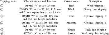
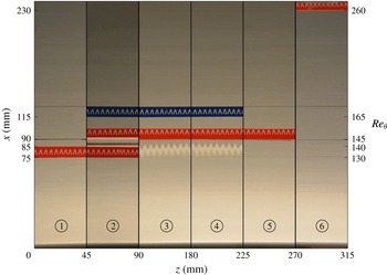
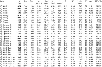
The boundary layer was tripped close to the leading edge with a set of tripping devices in order to obtain a range of different tripping conditions. Using as a reference the cases studied numerically by Schlatter & Örlü (Reference Schlatter and Örlü2012), a combination of weak, late, optimal and strong trippings was tested. In this study, the nomenclature optimal refers to cases in which the boundary layer is neither overstimulated nor understimulated by the tripping and where the profiles would lead to a common state within the streamwise distance considered here. With this aim, DYMO tapes (with the embossed letter ‘V’ pointing in the flow direction and a nominal height of 0.3 mm) in various combinations with and without turbulators were used to establish five different initial evolutions of the TBL. Additionally, a square bar with a side length of 5 mm was used to obtain a strongly overtripped case. The six different tripping cases under consideration are summarized in table 1, which also reports the colour coding used for these tripping conditions through the remainder of the paper and represented in figure 1. All of the tripping configurations were placed spanning the full spanwise length of the plate and at a streamwise location in the range $75<x~(\text{mm})<230$ from the leading edge, corresponding to the range $130<Re_{\unicode[STIX]{x1D703}}<260$ in terms of the laminar boundary layer, as can be observed in figure 1.

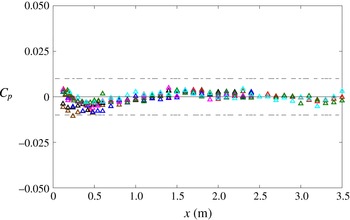
An initial set of four streamwise locations were selected for measurements on each tripping configuration. Additional stations were added to match $Re_{\unicode[STIX]{x1D703}}$ , covering a final Reynolds-number range of $440<Re_{\unicode[STIX]{x1D703}}<4070$ , as shown in table 3. The streamwise pressure-gradient distribution was controlled by adjusting the wind tunnel ceiling, which comprises a total of six panels allowing vertical displacement. The evolution of the pressure coefficient $C_{p}$ from the leading edge ( $x=0~\text{m}$ ) down to $x=3.5~\text{m}$ is shown in figure 2 for the six tripping cases under consideration, as well as for an additional case where no tripping was used (and where the boundary layer remained laminar). This figure shows the quality of the ZPG established in the test section, with $C_{p}$ values between $-0.01$ and 0.01, and deviations in $U_{\infty }$ below 0.5 %, which is comparable in quality to related studies, see, e.g., Marusic et al. (Reference Marusic, Chauhan, Kulandaivelu and Hutchins2015). From figure 2, it can be observed that the changes in displacement thickness $\unicode[STIX]{x1D6FF}^{\ast }$ due to the different tripping configurations have a very small influence on the pressure distribution. This is due to the large ratio between the distance from the flat plate to the tunnel ceiling (approximately 0.55 m) and the maximum displacement thickness, which was below approximately 1 %.

Table 1.

Specifications of the tripping configurations including location and respective colour coding for symbols. The embossed (DYMO) letter ‘V’ points downstream and has a nominal height of 0.3 mm.

Figure 1.

Schematic view of the tripping configurations used in the present study and summarized in table 1, with streamwise direction from bottom to top. The indicated momentum-thickness Reynolds number $Re_{\unicode[STIX]{x1D703}}$ is related to the laminar boundary layer in the absence of the trip. It should be noted that the difference between $\unicode[STIX]{x2462}$ and $\unicode[STIX]{x2463}$ is the height of the turbulator, and is hence not visible in the present two-dimensional view. The scale in mm is included in order to provide a reference for the size of the ‘V’ and the turbulator pattern.

Figure 2.

Streamwise variation of the pressure coefficient $C_{p}$ for the six tripping configurations considered in the present study. See table 1 for the colour code employed. The additional cyan symbols correspond to a case in which no tripping was used. Reference dashed lines at $C_{p}=\pm 0.010$ are included.

2.2 Hot-wire anemometry measurements

Streamwise velocity measurements were performed by means of a home-made single hot-wire probe resembling a standard Dantec boundary-layer probe, i.e. a 55P15. The hot-wire probe was etched in-house using a stubless platinum wire of $560~\unicode[STIX]{x03BC}\text{m}$ length and $2.5~\unicode[STIX]{x03BC}\text{m}$ nominal diameter, which was soldered to conical prongs with a diameter of approximately $30~\unicode[STIX]{x03BC}\text{m}$ . Voltage signals from the hot wire were recorded using a Dantec StreamLine 90N10 frame in conjunction with a 90C10 constant-temperature anemometer module operated at a resistance overheat ratio of 80 %. An offset and gain were applied to the top-of-the-bridge voltage in order to match the voltage range of the 16-bit A/D converter used. All of the measurements were recorded using a sampling frequency of 20 kHz and acquisition time of 30 s, and a low-pass filter of 10 kHz cutoff frequency was used prior to the data acquisition in order to avoid aliasing. Calibration of the hot wire was performed in situ using as reference a Prandtl tube located parallel to the incoming free stream. The Prandtl tube was connected to a micromanometer of type FC0510 (Furness Control Limited), which was also employed to record the ambient temperature and pressure during the calibration and the experiments. Data acquired in the calibration were fitted to a fourth-order polynomial curve, which is a rather common procedure in the wall-turbulence community (see, e.g., Morrison et al. 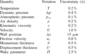Reference Morrison, McKeon, Jiang and Smits2004; Hultmark, Bailey & Smits Reference Hultmark, Bailey and Smits2010). Hot-wire measurements were acquired with a sufficiently large number of points within the sublayer and buffer region in order to correct for the absolute wall position and determine the friction velocity (Örlü & Vinuesa Reference Örlü, Vinuesa, Discetti and Ianiro2017) without relying on log-law constants. The composite profile given by Chauhan et al. (Reference Chauhan, Monkewitz and Nagib2009) was used to fit the experimental data and correct the absolute wall position as well as to obtain the friction velocity, which has been shown to be a robust method whenever near-wall measurements are at hand (Örlü, Fransson & Alfredsson Reference Örlü, Fransson and Alfredsson2010; Rodríguez-López, Bruce & Buxton Reference Rodríguez-López, Bruce and Buxton2015). Additional oil-film interferometry measurements, described in § 2.3, were performed for some selected conditions and were utilized to validate the aforementioned procedure to determine the friction velocity. The experimental uncertainties associated with the measurements were determined through an approach based on a Monte Carlo simulation, assuming random errors in the velocity measurements, viscosity and absolute wall position with the following uncertainties: 1 %, 0.2 % and $15~\unicode[STIX]{x03BC}\text{m}$ respectively (see, e.g., Bailey et al. Reference Bailey, Hultmark, Monty, Alfredsson, Chong, Duncan, Fransson, Hutchins, Marusic and McKeon2013). A summary of the resulting uncertainties is shown in table 2.

Table 2.

Uncertainty estimates for various measured quantities.

2.3 Oil-film interferometry measurements

Oil-film interferometry (OFI) was used to measure the wall-shear stress and validate the process to determine the friction velocity based on near-wall velocity measurements described in § 2.2. To this end, the OFI measurements were carried out at the same positions as the hot wire. Silicone oil with a nominal viscosity of 200 cSt at 25  $^{\circ }$ C was used. The oil viscosity was calibrated by means of a capillary-suspended level viscometer. Black Mylar films were attached to the flat plate in order to obtain better contrast for the fringe patterns from the oil-film light reflections. The oil film was illuminated using a low-pressure sodium lamp which had a power of 55 W and a nominal wavelength of 589 nm and was placed on the wind tunnel roof. A handheld digital thermocouple (Fluke) was attached to the flat plate close to the recording station to control the oil temperature. The equipment used to obtain the pictures consisted of a digital single-lens reflex camera (Nikon D7100) and a telephoto zoom lens (Nikon Nikkor 200 mm f4). The camera was placed on the roof of the wind tunnel at an angle of $15^{\circ }$ normal to the plate and was controlled remotely via a USB cable. For further details on the oil-film interferometry measurements performed, as well as on the post-processing of the data, the reader is referred to Örlü & Schlatter (Reference Örlü and Schlatter2013) and Vinuesa & Örlü (Reference Vinuesa, Örlü, Discetti and Ianiro2017) respectively. It should also be noted that we do not expect the very small local pressure gradient observed at approximately $x\simeq 0.4~\text{m}$ in figure 2 to impact the OFI results, since this technique has been used in other studies dealing with pressure-gradient TBLs (Monty, Harun & Marusic Reference Monty, Harun and Marusic2011; Vinuesa et al. Reference Vinuesa, Rozier, Schlatter and Nagib2014), where no effects that would produce a significant bias were observed.

Table 3.

Experimental parameters for all of the profiles in the present study. The measurement stations $x$ that are common to all of the trip configurations are highlighted in bold. The hot-wire length is denoted by $L$ , $\unicode[STIX]{x0394}t$ is the time between samples and $T$ is the total sampling time.

3.1 Comparison of TBLs at the same streamwise location

Figure 3.

Evolution of inner-scaled mean streamwise velocity (a,c,e,g,i,k) and variance (b,d,f,h,j,l) profiles at (◃) $x=0.24~\text{m}$ , (▵) $x=0.6~\text{m}$ , (▿) $x=1.1~\text{m}$ and (▹) $x=1.8~\text{m}$ . Colours correspond to the various tripping configurations described in table 1, while the solid line depicts the linear profile $U^{+}=y^{+}$ .

Mean streamwise velocity and velocity-fluctuation profiles are shown at four streamwise measuring stations for the six tripping cases in figure 3. For the tripping configurations from $\unicode[STIX]{x2460}$ to $\unicode[STIX]{x2464}$ , the near-wall region collapses in all of the stations, in agreement with the conclusions from Schlatter & Örlü (Reference Schlatter and Örlü2012), who showed that this region is expected to adapt quickly to a canonical TBL development. Interestingly, for case $\unicode[STIX]{x2465}$ (weak very late trip; panel (k)), in which the tripping is located at $x=0.23~\text{m}$ , corresponding to $Re_{\unicode[STIX]{x1D703}}=260$ , the boundary layer remains essentially laminar for $x<1.8~\text{m}$ , as apparent from the linear profile ( $U^{+}=y^{+}$ ) that extends far beyond the usual bound of $y^{+}\lesssim 5$ . The two optimal cases, $\unicode[STIX]{x2462}$ and $\unicode[STIX]{x2463}$ (panels (e) and (g)), exhibit similar developments in the buffer and overlap regions, with similar increase in $U_{\infty }^{+}$ at the same streamwise measurement stations, which indicates that the development of the outer region is adequate. (It should be noted that the missing point in the free stream present in one of the profiles from figure 3(e) is due to the fact that the traverse file was erroneously missing this point.) The weak tripping case $\unicode[STIX]{x2460}$ (panel (a)) shows that the first profile, at $x=0.24$  m, is slightly underdeveloped in comparison with the equivalent profile in the optimal tripping cases $\unicode[STIX]{x2462}$ and $\unicode[STIX]{x2463}$ : although the $U_{\infty }^{+}$ value is similar to that of case $\unicode[STIX]{x2463}$ , the overlap region deviates from the higher $Re$ profiles earlier (at $y^{+}\simeq 100$ ) compared with the optimal cases. The case $\unicode[STIX]{x2464}$ (panel (i)) exhibits a similar behaviour at $x=0.24$ , with an even lower value of the inner-scaled free-stream velocity related to the late transition and consequently lower friction Reynolds number $Re_{\unicode[STIX]{x1D70F}}$ . The profiles downstream of this station are, in the cases $\unicode[STIX]{x2460}$ and $\unicode[STIX]{x2464}$ , in good agreement with the optimal configurations $\unicode[STIX]{x2462}$ and $\unicode[STIX]{x2463}$ . With respect to the strong trip case $\unicode[STIX]{x2461}$ (panel (c)), the first profile at $x=0.24~\text{m}$ shows a more prominent wake region than the optimal cases, whereas at this first station the overlap region from case $\unicode[STIX]{x2461}$ is beneath the optimal ones. These effects become attenuated downstream, where the profiles from the strong trip case progressively converge towards the optimal ones.

Figure 4.

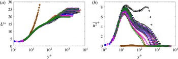
Inner-scaled (a) mean streamwise velocity and (b) variance profiles. Colours and symbols are as in figure 3, and additional measurement stations are represented by ( $\times$ )  $x=0.9$  m, (*) $x=0.95$  m, (▫) $x=2.1$  m and (○) $x=2.5$  m.

Regarding the streamwise variance profiles, the two optimal cases $\unicode[STIX]{x2462}$ and $\unicode[STIX]{x2463}$ also show an adequate development of the TBL, i.e. the inner and outer layers grow monotonically along the streamwise direction with only apparent differences in the first station. The mean flow deviation from the overlap region at approximately $y^{+}\simeq 100$ observed at the first station of case $\unicode[STIX]{x2460}$ is also observed in the variance profile; at this location, the variance decays faster than in the optimal case $\unicode[STIX]{x2463}$ . The case $\unicode[STIX]{x2464}$ also shows fluctuation amplitudes below the optimal cases in the outer region, but, interestingly, cases $\unicode[STIX]{x2460}$ and $\unicode[STIX]{x2464}$ progressively converge towards the variance profiles of the optimal cases, suggesting that they recover from the weak tripping adequately. With respect to the case $\unicode[STIX]{x2465}$ , the first profiles up to $x\simeq 1.8~\text{m}$ also indicate that the disturbance level is not sufficiently high to trigger transition to turbulence, as evinced from the fluctuation values close to zero throughout the whole boundary layer. The streamwise coordinate $x=1.8~\text{m}$ is the first one at which case $\unicode[STIX]{x2465}$ exhibits a near-wall fluctuation peak, although it clearly exhibits deviations with respect to the optimal cases. The first fluctuation profile from the strong tripping case $\unicode[STIX]{x2461}$ is interesting in that respect since, in addition to an enhanced value of the near-wall peak, it also shows the emergence of an outer peak at $y^{+}\simeq 250$ , although the wall-normal location is clearly beyond the inner layer, as is the case for a canonical high- $Re$ ZPG TBL (Alfredsson et al. Reference Alfredsson, Segalini and Örlü2011). These effects in the outer region of the boundary layer, reminiscent of adverse-pressure-gradient TBLs (Monty et al. Reference Monty, Harun and Marusic2011; Hosseini et al. Reference Hosseini, Vinuesa, Schlatter, Hanifi and Henningson2016; Bobke et al. 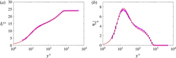Reference Bobke, Vinuesa, Örlü and Schlatter2017), were also observed by Tang et al. (Reference Tang, Jiang, Zheng and Wu2016) in their measurements of TBLs perturbed by a cylindrical roughness element. The outer peak in the fluctuation profiles progressively diminishes downstream of this location, as also observed by Tang et al. (Reference Tang, Jiang, Zheng and Wu2016), even if there is no complete convergence towards the optimal tripping profiles within the development lengths considered in the present study. These effects, together with the ones observed in the mean flow, can be further examined in figure 4, where all of the mean and variance profiles for all stations shown in table 3, including the ones not shown in figure 3, are presented. Moreover, the two optimal cases, i.e. 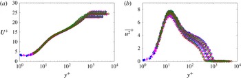cases $\unicode[STIX]{x2462}$ and $\unicode[STIX]{x2463}$ , are compared at a matched Reynolds number of $Re_{\unicode[STIX]{x1D703}}\simeq 2000$ with the DNS ZPG TBL data by Schlatter & Örlü (Reference Schlatter and Örlü2010) in figure 5. It should be noted that the experimental profiles are obtained at slightly different streamwise locations, i.e. at $x\simeq 0.90$  m in case $\unicode[STIX]{x2462}$ and at $x\simeq 0.95$  m in case $\unicode[STIX]{x2463}$ , in order to obtain the matched value of $Re_{\unicode[STIX]{x1D703}}$ . This figure shows that both cases with optimal tripping are in excellent agreement with the numerical data, a conclusion that is observed both in the mean velocity and in the streamwise velocity-fluctuation profiles. The results shown in figure 5 are in agreement with the conclusions reported by Schlatter & Örlü (Reference Schlatter and Örlü2012), in particular regarding the minimum value of $Re_{\unicode[STIX]{x1D703}}\simeq 2000$ necessary to converge towards canonical ZPG TBL conditions.

Figure 5.

Inner-scaled (a) mean streamwise velocity and (b) variance profiles corresponding to the two optimal cases, i.e. cases $\unicode[STIX]{x2462}$ and $\unicode[STIX]{x2463}$ , at $Re_{\unicode[STIX]{x1D703}}\simeq 2000$ . Colours and symbols are as in figure 4, with the addition of the solid red line which represents the DNS results by Schlatter & Örlü (Reference Schlatter and Örlü2010).

3.2 Comparison of TBLs at matched Reynolds number

Figure 6.

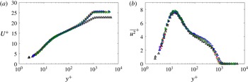
Inner-scaled (a) mean streamwise velocity and (b) velocity-fluctuation profiles at matched $Re_{\unicode[STIX]{x1D703}}\approx 1850$ for cases $\unicode[STIX]{x2460}$ , $\unicode[STIX]{x2461}$ , $\unicode[STIX]{x2463}$ and $\unicode[STIX]{x2465}$ . Colours and symbols are as in figure 3 and streamwise locations reported in table 1.

In order to emphasize the differences induced by the various tripping configurations under consideration, a comparison between cases at matched local momentum-thickness Reynolds numbers is shown. Figure 6 shows nominally matched $Re_{\unicode[STIX]{x1D703}}\approx 1850$ cases $\unicode[STIX]{x2460}$ , $\unicode[STIX]{x2461}$ , $\unicode[STIX]{x2463}$ and $\unicode[STIX]{x2465}$ . For the mean streamwise velocity and variance, the profiles of cases $\unicode[STIX]{x2460}$ , $\unicode[STIX]{x2463}$ and $\unicode[STIX]{x2465}$ are nearly identical. 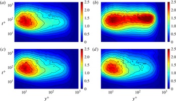In the strong trip case $\unicode[STIX]{x2461}$ , the profile exhibits a reduced wake region which shows that the influence of the initial condition, in the form of a strong overtripping, is still present. Regarding the premultiplied spectra of the streamwise velocity $f^{+}\unicode[STIX]{x1D6F7}_{uu}^{+}$ , which are shown in figure 7, good agreement between all of the cases, except $\unicode[STIX]{x2461}$ , can be observed in the near-wall region, where the inner peak is located at $y^{+}\simeq 15$ and at a streamwise wavelength of $\unicode[STIX]{x1D706}_{x}^{+}\simeq 1000$ (when the period $t^{+}$ is converted into a wavelength through the local mean velocity as convection velocity). In the strong trip case $\unicode[STIX]{x2461}$ , the large-scale motions are clearly energized by the bar, since a strong outer peak is present in the spectra. Similar results of agreement between cases $\unicode[STIX]{x2460}$ , $\unicode[STIX]{x2463}$ and $\unicode[STIX]{x2465}$ are observed also for $Re_{\unicode[STIX]{x1D703}}>3000$ . While the mean and variance profile for case $\unicode[STIX]{x2461}$ for $Re_{\unicode[STIX]{x1D703}}>3000$ is nearly indistinguishable from the other cases, differences remain in the spectral energy distribution in the outer layer when compared with the other tripping cases.

4.1 Existing criteria

In order to discern which profiles can be considered as canonical, the evolutions of the shape factor $H$ , the skin-friction coefficient $C_{f}$ and the wake parameter $\unicode[STIX]{x1D6F1}$ are considered as references. According to Chauhan et al. (Reference Chauhan, Monkewitz and Nagib2009), the wake parameter and the shape factor can be used as diagnostic quantities to assess whether a particular TBL can be considered to be canonical, since they have a high sensitivity to different boundary and inflow conditions. These quantities provide, in particular, an estimation of the degree of distortion in the outer part of the TBL, and require a long recovery distance to become independent of upstream disturbances (see also Schlatter & Örlü Reference Schlatter and Örlü2012). In this study, the reference curve chosen to characterize the shape factor is the one proposed by Monkewitz, Chauhan & Nagib (Reference Monkewitz, Chauhan and Nagib2007), which is obtained from asymptotic arguments, based on a vast number of experimental profiles covering a wide range of Reynolds numbers, $450<Re_{\unicode[STIX]{x1D703}}<125\,000$ . The equation proposed by Monkewitz et al. (Reference Monkewitz, Chauhan and Nagib2007) relates $H$ and $Re_{\unicode[STIX]{x1D703}}$ as follows:

with $\unicode[STIX]{x1D705}=0.384$ , $I_{WW}=7.11$ and $C=3.3$ . Regarding the evolution of the skin-friction coefficient $C_{f}$ , the following Coles–Fernholz relation is considered:

where the value of the von Kármán coefficient $\unicode[STIX]{x1D705}$ is also $0.384$ and the constant $C^{\prime }$ takes the value $4.127$ . This choice of constants is due to Nagib, Chauhan & Monkewitz (Reference Nagib, Chauhan and Monkewitz2007), who established them based on a comprehensive analysis of experimental databases. Finally, the baseline streamwise evolution of the wake parameter $\unicode[STIX]{x1D6F1}$ is obtained following the methodology proposed by Chauhan et al. (Reference Chauhan, Monkewitz and Nagib2009) based on the integration of the composite profile.

4.2 Diagnostic-plot criterion

The previous criteria rely on the computation of integral quantities, which often requires previous knowledge of other variables such as an accurate determination of the absolute wall position $y$ and the friction velocity $u_{\unicode[STIX]{x1D70F}}$ . These parameters are typically highly sensitive to experimental errors (Örlü et al. Reference Örlü, Fransson and Alfredsson2010). Moreover, the Reynolds-number evolution of other reference quantities such as $H$ or $\unicode[STIX]{x1D6F1}$ can be defined in terms of several empirical curves. Furthermore, the application of the criteria described in § 4.1 requires also an extensive experimental campaign (in terms of skin-friction and detailed mean velocity profile measurements), as well as intensive data processing, to identify whether and from which streamwise location on the TBL can be considered as well-behaved. For these reasons, here we propose an alternative method based on the so-called diagnostic-plot scaling introduced by Alfredsson et al. (Reference Alfredsson, Segalini and Örlü2011). In this scaling, the root mean square of the streamwise velocity fluctuation $u^{\prime }$ is plotted against the mean velocity $U$ , both normalized by the free-stream velocity $U_{\infty }$ . This plot has been shown to scale canonical ZPG TBL data over a wide range of $Re$ throughout the logarithmic and outer region of ZPG TBLs (Alfredsson, Örlü & Segalini Reference Alfredsson, Örlü and Segalini2012; Örlü et al. Reference Örlü, Segalini, Klewicki and Alfredsson2016). The diagnostic plot was also found to scale pressure-gradient turbulent boundary layers (Drózdz, Elsner & Drobniak Reference Drózdz, Elsner and Drobniak2015) and thereby provide a robust method to determine the boundary-layer thickness and the edge velocity in these flows (Vinuesa et al. Reference Vinuesa, Bobke, Örlü and Schlatter2016a ), and scale rough-wall boundary layers (Castro, Segalini & Alfredsson Reference Castro, Segalini and Alfredsson2013) as well as a variety of wall-bounded and free-shear flows (Castro Reference Castro2015). One of the greatest advantages of this scaling is the fact that, according to Alfredsson et al. (Reference Alfredsson, Segalini and Örlü2011), the data for a canonical ZPG TBL collapse in the outer region, especially in the range $0.7\leqslant U/U_{\infty }\leqslant 0.9$ (the lower limit further decreases with increasing $Re$ , see Örlü et al. Reference Örlü, Segalini, Klewicki and Alfredsson2016), following a linear relation,

where $\unicode[STIX]{x1D6FC}$ and $\unicode[STIX]{x1D6FD}$ are fitting parameters. This means that the profiles that follow (4.3) in the outer region give ‘a good indication whether the boundary layer is in a natural state’ (Alfredsson & Örlü Reference Alfredsson and Örlü2010). Although this was suggested in the first work on the diagnostic plot, it has not been systematically investigated with the focus on tripping and inflow effects as in the present work. The effect of $Re_{\unicode[STIX]{x1D703}}$ on the values of the parameters $\unicode[STIX]{x1D6FC}$ and $\unicode[STIX]{x1D6FD}$ is analysed in the following and is used to assess whether a boundary layer is considered to be well-behaved or not. It should be noted that the only data required to use this method are $U$ and $u^{\prime }$ in the outer region, and $U_{\infty }$ . These measurements can be obtained easily at numerous stations from a simple hot-wire scan, without the need for any additional measurement such as $y$ , $u_{\unicode[STIX]{x1D70F}}$ , etc. Furthermore, measurements of turbulence quantities in the outer region are generally not subjective to spatial or temporal resolution issues. Therefore, this approach could be suitable to assess the development of TBLs in a robust and efficient manner.

4.3 Validation of the diagnostic-plot method with numerical data

Table 4.

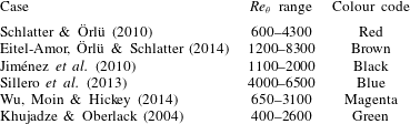
Summary of the numerical databases under consideration in the present study, together with $Re_{\unicode[STIX]{x1D703}}$ range and colour code.

Figure 8.

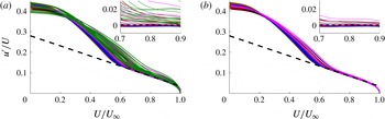
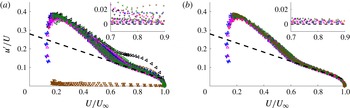
Diagnostic plot for (a) all of the numerical data sets and (b) the numerical data sets that are considered to be well-behaved. The colours correspond to the cases summarized in table 4. The dashed line represents (4.3) with $\unicode[STIX]{x1D6FC}=0.280$ and $\unicode[STIX]{x1D6FD}=0.245$ . The insets depict the difference between the data and (4.3) with the aforementioned constants.

Figure 9.

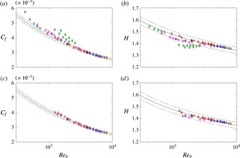
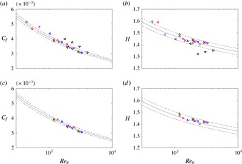
Skin-friction coefficient evolution with $Re_{\unicode[STIX]{x1D703}}$ for (a) all of the numerical data sets and (c) the numerical profiles that follow the diagnostic-plot scaling given by (4.3), where the solid line is the reference given by (4.2) and $\pm 3\,\%$ deviation is represented by the dashed lines. Reynolds-number evolution of the shape factor $H$ is given for (b) all of the numerical cases and (d) the numerical profiles that follow (4.3), where the solid line shows the reference trend given by (4.1) and the dashed lines show $\pm 2\,\%$ deviation. The colours correspond to the cases summarized in table 4.

Figure 10.

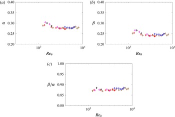
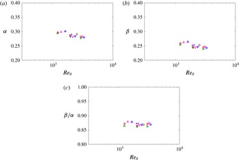
Evolution of the diagnostic-fit coefficients (a) $\unicode[STIX]{x1D6FC}$ and (b) $\unicode[STIX]{x1D6FD}$ , as well as the ratio (c) $\unicode[STIX]{x1D6FD}/\unicode[STIX]{x1D6FC}$ , with $Re_{\unicode[STIX]{x1D703}}$ . These coefficients are obtained from fits to (4.3), from the numerical databases described in table 4, where the colour code is also given.

In order to evaluate the ability of the method described in § 4.2 to assess the convergence towards a canonical state of TBLs, here, the method is applied to a number of ZPG TBL DNS data sets, namely the ones by Khujadze & Oberlack (Reference Khujadze and Oberlack2004), Jiménez et al. (Reference Jiménez, Hoyas, Simens and Mizuno2010), Schlatter & Örlü (Reference Schlatter and Örlü2010), Sillero et al. (Reference Sillero, Jiménez and Moser2013) and Wu et al. (Reference Wu, Moin and Hickey2014), and to the well-resolved large-eddy simulation (LES) database by Eitel-Amor et al. (Reference Eitel-Amor, Örlü and Schlatter2014). It should be noted that the particular $Re_{\unicode[STIX]{x1D703}}$ ranges of the various databases can be found in table 4. The values of the free-stream velocity $U_{\infty }$ , the $99\,\%$ boundary-layer thickness $\unicode[STIX]{x1D6FF}_{99}$ as well as other boundary-layer parameters have been recomputed following the procedure as outlined for the tripping experiments. In figure 8, the numerical data are plotted in the diagnostic-plot form: panel (a) reports the profiles at all stations while panel (b) reports only the profiles that fit to the diagnostic-plot outer scaling. In order to identify which profiles follow the diagnostic plot, only the profiles complying with both the $H$ and $C_{f}$ criteria to within $\pm$ 2 % and 3 % tolerance respectively have been considered, and fitting curves for $\unicode[STIX]{x1D6FC}$ and $\unicode[STIX]{x1D6FD}$ as function of $Re_{\unicode[STIX]{x1D703}}$ have been computed with the remaining data points. Then, only the profiles with $\unicode[STIX]{x1D6FC}$ , $\unicode[STIX]{x1D6FD}$ and $\unicode[STIX]{x1D6FD}/\unicode[STIX]{x1D6FC}$ complying with the fitting relations to within $\pm$ 5 %, $\pm$ 5 % and $\pm$ 2 % tolerance respectively have been considered to properly fit the diagnostic plot (cf. § 4.4). On the other hand, the $H$ and $C_{f}$ evolutions corresponding to all of the numerical data sets are shown in figure 9, together with the reference curves given by (4.1) and (4.2) respectively, as described in § 4.1. It is interesting to note that the profiles that satisfy the diagnostic-plot criterion, i.e. the ones shown in figure 8(b), are identical to the ones that follow the reference $H$ and $C_{f}$ curves within $\pm 2\,\%$ and 3 % tolerances respectively, as shown in figure 9. In accordance with previous studies (Schlatter & Örlü Reference Schlatter and Örlü2010, Reference Schlatter and Örlü2012), the diagnostic plot indicates that all of the profiles from Khujadze & Oberlack (Reference Khujadze and Oberlack2004) exhibit non-canonical behaviour. The general agreement between the results from the inspection of the diagnostic plot and the criteria by Chauhan et al. (Reference Chauhan, Monkewitz and Nagib2009) is an argument in favour of the diagnostic-plot criterion described in § 4.2 as a robust tool to assess whether a particular boundary layer exhibits canonical ZPG TBL conditions. In fact, the diagnostic plot can be used not only to discern well-behaved profiles, but also to recognize whether a profile is fully developed. From the insets of figure 8, it can be observed that with increasing $Re_{\unicode[STIX]{x1D703}}$ , the profiles tend to collapse. This fact can be better understood when the coefficients $\unicode[STIX]{x1D6FC}$ and $\unicode[STIX]{x1D6FD}$ of (4.3) are plotted as a function of $Re_{\unicode[STIX]{x1D703}}$ , as is done in figure 10. It should be noted that these coefficients, obtained through fitting each individual profile to (4.3), exhibit an asymptotic behaviour with $Re$ , i.e. $\unicode[STIX]{x1D6FC}$ and $\unicode[STIX]{x1D6FD}$ converge towards values of approximately 0.280 and 0.245 respectively for $Re_{\unicode[STIX]{x1D703}}>2000$ . This observation is in accordance with the results by Schlatter & Örlü (Reference Schlatter and Örlü2012), who established $Re_{\unicode[STIX]{x1D703}}\simeq 2000$ as a threshold beyond which canonical features are exhibited by the ZPG TBL profiles, for cases in which transition was initiated at $Re_{\unicode[STIX]{x1D703}}<300$ . Moreover, Sillero et al. (Reference Sillero, Jiménez and Moser2013) also claimed that the profiles with $Re_{\unicode[STIX]{x1D703}}<2000$ could not be considered to be fully developed. Interestingly, figure 10 also shows that the ratio $\unicode[STIX]{x1D6FD}/\unicode[STIX]{x1D6FC}$ has an approximately constant value of approximately 0.876 for $Re_{\unicode[STIX]{x1D703}}>1000$ , which is the ratio of the asymptotic values of the two coefficients; it should be noted that values are rounded to two decimal places.

4.4 Determination of the canonical boundary layer from experimental data

After showing the ability of the diagnostic-plot method described in § 4.2 to discern which numerical profiles exhibited canonical ZPG TBL conditions, we applied the same methodology to the experimental measurements to assess whether its results are in agreement with the other criteria described in § 4.1. In figure 11, all of the experimental profiles summarized in table 1 are presented in the diagnostic-plot form: panel (a) reports all cases, while panel (b) only reports the cases that follow the diagnostic scaling. Plotting now the profiles that remain in figure 11(b) in classical inner scaling for the mean and variance, figure 4 reduces to figure 12, which exhibits the expected clear Reynolds-number trends in the wake profile for the mean velocity profile as well as the increase of the near-wall peak in the variance profile and the monotonic increase of the turbulence level in the outer layer.

Figure 11.

Diagnostic plot for (a) all of the experimental profiles and (b) the experimental profiles that follow the diagnostic-plot scaling given by (4.3). The colours correspond to the cases summarized in table 1. The dashed line represents (4.3) with $\unicode[STIX]{x1D6FC}=0.280$ and $\unicode[STIX]{x1D6FD}=0.245$ . The insets depict the difference between the data and (4.3) with the aforementioned constants.

Figure 12.

Inner-scaled (a) mean streamwise velocity and (b) variance profiles. The same data as in figure 4 are shown, with the difference that profiles not passing the diagnostic-plot criteria are omitted.

Figure 13.

Skin-friction coefficient evolution with $Re_{\unicode[STIX]{x1D703}}$ for (a) all of the experimental profiles and (c) the experimental profiles that follow the diagnostic-plot scaling given by (4.3), where the solid line is the reference given by (4.2) and $\pm 3\,\%$ tolerances are represented by the dashed lines. Reynolds-number evolution of the shape factor $H$ is given for (b) all of the experimental cases and (d) the experimental profiles that follow (4.3), where the solid line shows the reference trend given by (4.1) and the dashed lines show $\pm 2\,\%$ deviation. The colours correspond to the cases summarized in table 3.

Figure 14.

Evolution of the diagnostic-plot coefficients (a) $\unicode[STIX]{x1D6FC}$ and (b) $\unicode[STIX]{x1D6FD}$ , as well as (c) the ratio $\unicode[STIX]{x1D6FD}/\unicode[STIX]{x1D6FC}$ , with $Re_{\unicode[STIX]{x1D703}}$ . These coefficients are obtained from fits to (4.3), from the experimental databases described in table 3, where the colour code is also given.

Figure 13 depicts the Reynolds-number evolution of both $C_{f}$ and $H$ , and it is interesting to observe that, as in the numerical databases, the experimental profiles that follow the diagnostic-plot scaling are the ones consistent with the reference curves for both the skin-friction coefficient and the shape factor, as described in § 4.1. All profiles that do not follow the diagnostic-plot criterion fail according to either the $C_{f}$ or the $H$ based criterion. For example, it can be observed that the cases that fulfil the $H$ criterion (such as the lowest $Re$ profile from the strong overtripping case  $\unicode[STIX]{x2461}$ ) but not the $C_{f}$ criterion are clearly discarded by the diagnostic-plot approach. Therefore, the proposed methodology can also be used in experimental databases to assess the degree of convergence towards canonical conditions of a particular TBL configuration. Further support for this statement is given in figure 14, where the coefficients from the diagnostic-plot equation (4.3) are calculated and shown as a function of $Re_{\unicode[STIX]{x1D703}}$ . Also in this case the profiles with $Re_{\unicode[STIX]{x1D703}}>2000$ exhibit coefficients that asymptote to $\unicode[STIX]{x1D6FC}\simeq 0.280$ and $\unicode[STIX]{x1D6FD}\simeq 0.245$ . Interestingly, also in the experimental profiles, the ratio $\unicode[STIX]{x1D6FD}/\unicode[STIX]{x1D6FC}$ exhibits an approximately constant value of approximately 0.876 throughout the whole Reynolds-number range, as in the numerical databases shown in § 4.3.

The evolution of the $\unicode[STIX]{x1D6FC}$ and $\unicode[STIX]{x1D6FD}$ coefficients is extended to higher Reynolds numbers by including in the analysis the experimental data sets by Bailey et al. (Reference Bailey, Hultmark, Monty, Alfredsson, Chong, Duncan, Fransson, Hutchins, Marusic and McKeon2013), Örlü & Schlatter (Reference Örlü and Schlatter2013) and Vincenti et al. (Reference Vincenti, Klewicki, Morrill-Winter, White and Wosnik2013) (except the highest $Re$ data due to scatter and a limited number of data points in the region in which $\unicode[STIX]{x1D6FC}$ and $\unicode[STIX]{x1D6FD}$ are determined). It should be noted that in the extended database, the maximum $Re_{\unicode[STIX]{x1D703}}$ is approximately 40 000. Following the same approach as in figure 14, the diagnostic-plot coefficients are calculated for all of the data sets from tables 3 and 4, and for the three additional high- $Re$ experimental data sets. 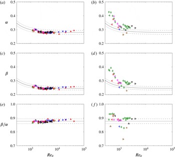In figure 15, the Reynolds-number evolutions of the coefficients $\unicode[STIX]{x1D6FC}$ and $\unicode[STIX]{x1D6FD}$ , together with that of the ratio $\unicode[STIX]{x1D6FD}/\unicode[STIX]{x1D6FC}$ , are shown for all of the cases under consideration. Panels (a,c,e) show the cases where the particular profile follows the diagnostic-plot scaling, and panels (b,d,f) show the cases where the profiles do not follow it. It is interesting to note that all of the high- $Re$ data sets exhibit asymptotic values of $\unicode[STIX]{x1D6FC}$ , $\unicode[STIX]{x1D6FD}$ and $\unicode[STIX]{x1D6FD}/\unicode[STIX]{x1D6FC}$ , which are consistent with the conclusions drawn from the previous lower- $Re$ data sets. Excluding the profiles in panels (b,d,f), which do not follow the diagnostic scaling, it is possible to establish the following empirical fits defining the $Re_{\unicode[STIX]{x1D703}}$ evolutions of $\unicode[STIX]{x1D6FC}$ and $\unicode[STIX]{x1D6FD}$ :

These curves are also shown in figure 15, where it can be observed that all of the profiles in panels (a) and (c) follow these trends within $\pm 5\,\%$ . Moreover, figure 15(e) shows that the ratio $\unicode[STIX]{x1D6FD}/\unicode[STIX]{x1D6FC}$ is approximately constant and equal to $\simeq 0.876$ for the whole $Re$ range in all of the profiles following the diagnostic scaling. All of the profiles in this panel exhibit deviations in $\unicode[STIX]{x1D6FD}/\unicode[STIX]{x1D6FC}$ within $\pm 2\,\%$ with respect to 0.876, which is an interesting conclusion regarding the applicability of the diagnostic-plot method for assessment of well-behaved profiles at low $Re$ . With respect to the profiles shown in figure 15(b,d,f), it is clear that $\unicode[STIX]{x1D6FC}$ and $\unicode[STIX]{x1D6FD}$ do not follow the relations given by (4.4) and (4.5), and the ratio $\unicode[STIX]{x1D6FD}/\unicode[STIX]{x1D6FC}$ deviates from 0.876. Interestingly, the cases that do not satisfy the diagnostic-plot scaling are not consistent with the $C_{f}$ and $H$ (4.2) and (4.1) presented above either, which shows additional support for the use of the methodology based on the diagnostic-plot method, and additionally highlights the consistency of the various approaches to characterize the TBL development. In fact, there are few cases in figure 15(b,d,f) in which the trend of a particular coefficient is followed, but only the profiles for which the evolutions of the two coefficients are consistent with the empirical fits also satisfy both the skin-friction and shape-factor criteria.

Figure 15.

Evolution with $Re_{\unicode[STIX]{x1D703}}$ of diagnostic-plot coefficients (a,b) $\unicode[STIX]{x1D6FC}$ and (c,d) $\unicode[STIX]{x1D6FD}$ from (4.3), as well as (e,f) their ratio $\unicode[STIX]{x1D6FD}/\unicode[STIX]{x1D6FC}$ , for all experimental and numerical (indicated by ♢) data sets summarized in tables 3 and 4 respectively. Additional high- $Re$ experimental data sets are represented by the following symbols: (blue star) Bailey et al. (Reference Bailey, Hultmark, Monty, Alfredsson, Chong, Duncan, Fransson, Hutchins, Marusic and McKeon2013), (black star) Örlü & Schlatter (Reference Örlü and Schlatter2013) and (red star) Vincenti et al. (Reference Vincenti, Klewicki, Morrill-Winter, White and Wosnik2013). Panels (a,c,e) show the profiles that follow the diagnostic-plot scaling (4.3), whereas the data shown in panels (b,d,f) do not follow it. Black solid lines represent the empirical fits for $\unicode[STIX]{x1D6FC}$ and $\unicode[STIX]{x1D6FD}$ given by (4.4) and (4.5) respectively, as well as the ratio $\unicode[STIX]{x1D6FD}/\unicode[STIX]{x1D6FC}\simeq 0.876$ . Dashed lines represent $\pm 5\,\%$ deviation with respect to (4.4) and (4.5), and $\pm 2\,\%$ deviation with respect to $\unicode[STIX]{x1D6FD}/\unicode[STIX]{x1D6FC}\simeq 0.876$ .

Figure 16.

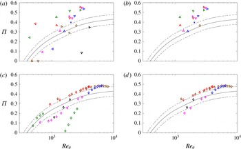
Reynolds-number evolution of the wake parameter $\unicode[STIX]{x1D6F1}$ from (a) all of the experimental profiles summarized in table 3, (b) the profiles that follow the diagnostic-plot scaling (4.3), (c) all of the numerical data sets and (d) the numerical data sets that follow the diagnostic-plot scaling given by (4.3). The solid line is obtained through integration of the composite profile as in Chauhan et al. (Reference Chauhan, Monkewitz and Nagib2009) and the dashed lines represent $\pm$ 0.05 deviation.

Figure 17.

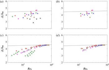
Reynolds-number evolution of $\unicode[STIX]{x1D6E5}/\unicode[STIX]{x1D6FF}_{99}$ from (a) all of the experimental profiles summarized in table 3, (b) the experimental profiles that follow the diagnostic-plot scaling (4.3), (c) all of the numerical data sets and (d) the numerical data sets that follow the diagnostic-plot scaling given by (4.3). The solid line shows the reference trend given by Nagib et al. (Reference Nagib, Chauhan and Monkewitz2007).

The discussion above shows that the diagnostic-plot criterion, which only requires measurements of the streamwise mean velocity and turbulence intensity, is consistent with other methods such as the skin-friction coefficient curve, which requires accurate measurements of the wall-shear stress, or the shape-factor curve, for which full velocity profile measurements are required. It should be noted that it may not be straightforward to determine the location of the wall directly and/or accurately in hot-wire measurements, especially at high Reynolds numbers where the viscous length scale becomes progressively smaller (Örlü et al. Reference Örlü, Fransson and Alfredsson2010; Vinuesa, Duncan & Nagib Reference Vinuesa, Duncan and Nagib2016b ). For this reason, in the present work, we propose a methodology based on the diagnostic plot given by (4.3), and the evolution with $Re$ of its parameters. In order to discern whether a ZPG TBL is well-behaved, it is only necessary to analyse the mean velocity and turbulence intensity profiles in the range $0.7<U/U_{\infty }<0.9$ , where a linear fit can be used to obtain the values of $\unicode[STIX]{x1D6FC}$ , $\unicode[STIX]{x1D6FD}$ and $\unicode[STIX]{x1D6FD}/\unicode[STIX]{x1D6FC}$ . These parameters can be compared with (4.4) and (4.5) for $\unicode[STIX]{x1D6FC}$ and $\unicode[STIX]{x1D6FD}$ , and with the value 0.876 for the ratio $\unicode[STIX]{x1D6FD}/\unicode[STIX]{x1D6FC}$ . As shown in figure 15, if the values of $\unicode[STIX]{x1D6FC}$ and $\unicode[STIX]{x1D6FD}$ lie within $\pm 5\,\%$ of the values predicted by (4.4) and (4.5), and if $\unicode[STIX]{x1D6FD}/\unicode[STIX]{x1D6FC}$ is within $\pm 2\,\%$ of 0.876, the ZPG TBL profile can be considered to be well-behaved. It should be noted that since the trends discussed above are valid for $Re_{\unicode[STIX]{x1D703}}>1000$ , in cases where $Re_{\unicode[STIX]{x1D703}}$ is unknown, the procedure to ensure convergence towards a canonical state is to obtain $\unicode[STIX]{x1D6FC}$ , $\unicode[STIX]{x1D6FD}$ and $\unicode[STIX]{x1D6FD}/\unicode[STIX]{x1D6FC}$ at several streamwise locations and study the convergence of these values towards the predicted asymptotic values, i.e. $\unicode[STIX]{x1D6FC}\simeq 0.280$ and $\unicode[STIX]{x1D6FD}\simeq 0.245$ . The use of the diagnostic-plot methodology proposed here shows the advantage with respect to the shape-factor method of relying only on the scaling of mean velocity and turbulence intensity in the outer region of the TBL. Moreover, the method proposed by Chauhan et al. (Reference Chauhan, Monkewitz and Nagib2009) based on the wake parameter $\unicode[STIX]{x1D6F1}$ is also tested here, and compared with the outcome of the other methods discussed above. It should be noted that the wake parameter is a very sensitive quantity, which requires accurate measurements of the inner-scaled mean velocity profile (including $u_{\unicode[STIX]{x1D70F}}$ and $y$ ), relies on composite fits to calculate the value of $\unicode[STIX]{x1D6F1}$ and is directly dependent on the log-law constants/coefficients, an issue of ambiguity on its own for low- $Re$ data sets. In figure 16(a), we show the evolution with $Re$ of the wake parameter calculated from all of the experimental profiles. It should be noted that the calculation of $\unicode[STIX]{x1D6F1}$ was performed based on the method proposed by Chauhan et al. (Reference Chauhan, Monkewitz and Nagib2009) and the reference $\unicode[STIX]{x1D6F1}$ evolution with $Re_{\unicode[STIX]{x1D703}}$ was determined through integration of the composite profile proposed in the same work. On the other hand, in figure 16(b), we show the $\unicode[STIX]{x1D6F1}$ curve from the profiles that satisfy the diagnostic-plot criterion (which also satisfy the skin-friction and shape-factor criteria, as discussed above). As expected, the profiles that do not satisfy the diagnostic-plot method also deviate from the $\unicode[STIX]{x1D6F1}$ curve proposed by Chauhan et al. (Reference Chauhan, Monkewitz and Nagib2009), and do not exhibit any consistent trend with Reynolds number. Furthermore, the profiles that follow the diagnostic-plot method exhibit an increasing trend of $\unicode[STIX]{x1D6F1}$ with $Re_{\unicode[STIX]{x1D703}}$ , similar to the one shown by the curve from Chauhan et al. (Reference Chauhan, Monkewitz and Nagib2009), although they appear to be consistently shifted upwards by approximately $\simeq ~0.1$ . This shows that, although the wake parameter is also a good indicator of the state of the boundary layer, and in particular of its convergence towards canonical ZPG TBL conditions, it is very sensitive to a number of factors and experimental uncertainties, including details of the tripping mechanism and the fit, and therefore shows more difficulties when used to assess in detail the conditions of the TBL. It should also be noted that the $\unicode[STIX]{x1D6F1}$ values given here (in accordance with Chauhan et al. Reference Chauhan, Monkewitz and Nagib2009) are obtained with fixed log-law parameters, which explains why very low and even negative values can be obtained; cf. the values in table 3. To underline this point, panels (c) and (d) depict the same plots for the DNS data discussed in § 4.3, which besides removing data points with low $Re$ -effects also indicate that most of the data sets lie actually above, but parallel to, the curve from Chauhan et al. (Reference Chauhan, Monkewitz and Nagib2009), in accordance with the experimental data shown in panels (a) and (b).

In addition to the $\unicode[STIX]{x1D6F1}$ criterion, the evolution of the Rotta–Clauser length scale $\unicode[STIX]{x1D6E5}=U_{\infty }\unicode[STIX]{x1D6FF}^{\ast }/u_{\unicode[STIX]{x1D70F}}$ normalized with the boundary-layer thickness defined here as $\unicode[STIX]{x1D6FF}_{99}$ is also studied. According to the work by Nagib et al. (Reference Nagib, Chauhan and Monkewitz2007), the ratio $\unicode[STIX]{x1D6E5}/\unicode[STIX]{x1D6FF}_{99}$ can also be used to assess the evolution of a TBL towards a well-behaved state independent of the inflow conditions. In figure 17(a,c), we show the Reynolds-number evolution of $\unicode[STIX]{x1D6E5}/\unicode[STIX]{x1D6FF}_{99}$ for all of the experimental and numerical cases under consideration, where it can be observed that a number of profiles exhibit $\unicode[STIX]{x1D6E5}/\unicode[STIX]{x1D6FF}_{99}$ values below the trend reported by Nagib et al. (Reference Nagib, Chauhan and Monkewitz2007). This is associated with profiles that have not reached a state independent of the inflow conditions, and are therefore subject to non-equilibrium effects. In figure 17(b,d), we only show the experimental and numerical profiles that follow the diagnostic-plot scaling given by (4.3). It can be observed that the profiles above $Re_{\unicode[STIX]{x1D703}}\simeq 2000$ are in good agreement with the curve developed by Nagib et al. (Reference Nagib, Chauhan and Monkewitz2007), whereas the ones below this Reynolds number follow a similar trend, with slightly lower values. It should also be noted that the higher- $Re$ profiles exhibit a value of $\unicode[STIX]{x1D6E5}/\unicode[STIX]{x1D6FF}_{99}$ approximately equal to 4.5, which is consistent with the observations by Nagib et al. (Reference Nagib, Chauhan and Monkewitz2007). Therefore, the method proposed in the present work based on the diagnostic plot is in reasonably good agreement with the approach to assess well-behaved profiles based on $\unicode[STIX]{x1D6E5}/\unicode[STIX]{x1D6FF}_{99}$ proposed by Nagib et al. (Reference Nagib, Chauhan and Monkewitz2007).

Figure 18.

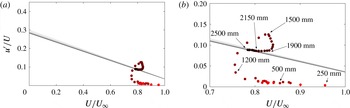
(a) Diagnostic-plot methodology as a design tool, demonstrated using the ZPG TBL with the tripping configuration $\unicode[STIX]{x2465}$ , i.e. the weak very late tripping. The solid lines correspond to (4.4)–(4.5) with $Re_{\unicode[STIX]{x1D703}}=1000$ (light grey) to 10 000 (dark grey) (10 logarithmically spaced cases). (b) Zoom-in of (a) with the indicated streamwise locations of the measurement points taken with equidistant streamwise spacings of $\unicode[STIX]{x0394}x=50~\text{m}$ .

4.5 Diagnostic-plot methodology as a design tool

The previous sections have shown that the proposed diagnostic-plot methodology is a reliable technique to evaluate the development of ZPG TBLs towards canonical conditions, which only requires measurements of the streamwise mean and turbulence intensity in the outer region of the boundary layer. Since neither the skin-friction coefficient, shape factor or wake parameter, nor full velocity profile measurements are required, the idea to assess the streamwise development with a scan through the outer part of the TBL arose. More specifically, here, we demonstrate that by placing a hot-wire probe within the outer part of the boundary layer and traversing it downstream by keeping it within the outer region of the TBL, the streamwise location from where on the TBL can be considered to be genuine and well-behaved is estimated to be when the measured turbulence intensity falls on relation (4.3) with the established constants. Figure 18 shows the results from a streamwise traverse while keeping (through an iterative procedure) the probe within the velocity range $0.7<U/U_{\infty }<0.9$ through the outer part of a ZPG TBL corresponding to the tripping configuration $\unicode[STIX]{x2465}$ . As is apparent from the colour-coded measurement points, indicating the streamwise distance from the leading edge (from lighter to darker symbols with increasing streamwise distance), the boundary layer is first laminar and then undergoes transition to turbulence with the associated overshoot in turbulence intensity (in accordance with figure 3 k,l) somewhere between the 1.1 m and 1.8 m stations. Since the measurement points are taken with an equidistant streamwise spacing, it is apparent from the accumulation of measurement points that the outer layer requires large development lengths to overcome the post-transitional stage and behave in accordance with the diagnostic scaling. It is interesting to note that the profiles in the post-transitional regime for $x\geqslant 1.8$  m actually agree very well with the empirical curves for the skin-friction coefficient, shape factor and wake parameter. According to the diagnostic plot, the first point that complies with the diagnostic scaling corresponds to $x=1.90$  m, which agrees sufficiently well with the results shown in figure 13. It should be noted that, albeit the exact location of the range $0.7<U/U_{\infty }<0.9$ is not known a priori, the traverse can still be taken in an automated way by iterating until the measured mean velocity is within the desired percentage of the free-stream velocity.