

I. INTRODUCTION
Among the many innovations in the work of Henry Ludwell Moore is his use of Joseph Fourier’s harmonic analysis to examine the cyclical behavior of time series. Unlike his use of regression analysis, however, this aspect of his work has received relatively little attention from historians of economic and econometric thought. Indeed, George Stigler, in his review of Moore’s lifetime body of work, states, “Moore’s work on cycles has left no imprint on present day economics, and by this most basic of tests it must be judged a complete failure” (Stigler Reference Stigler1962, p. 12). The lack of impact may reflect the fact that, while regression analysis has become the dominant tool of applied economics, Fourier analysis has become something of a niche area. As documented in the recent work of Terry Mills (Reference Mills2011), modern time series analysis in economics is mainly conducted in the time domain, which focuses on the covariances of a time series at different dates, rather than the frequency domain, which views a time series as a weighted sum of periodic (or cyclical) functions. The kind of analysis conducted by Moore (Reference Moore1914, chs. 2 and 3; and Reference Moore1923, chs. 3–5) in two key contributions to econometric methodology, which initially looked to be a promising approach to time series analysis, has been superseded by the use of ARIMA modeling. Of course, the fact that Moore’s work in this area has been generally ignored by modern economists may also reflect his identification of the transits of Venus as the primary exogenous factor driving terrestrial economic cycles.Footnote 1 In addition to being largely disregarded, Moore’s Fourier analysis also received scornful criticism; economists have even argued that Moore may have incorrectly applied the technique.Footnote 2
On the contrary, in this paper we argue that Moore’s work using the frequency domain deserves more attention from historians of the econometric method. Even simply by using a methodology that, prior to his work, had not been applied to economic problems, Moore deserves credit for a significant innovation. Moreover, his work marks an imaginative and innovative use of the method, which generates results that remain interesting and deserving of further investigation. The idea that Moore’s theory of economic cycles was strongly influenced by the transfer of periodogram analysis from physics to economics is well documented by, for instance, Philippe Le Gall (Reference Le Gall1999). However, we show in this paper that his use of Arthur Schuster’s (Reference Schuster1898, pp. 13–14) periodogram is in fact not standard. By modifying the way in which frequencies are calculated and identified, Moore allows for more precise identification of long frequency cycles. We also note that Moore’s model of the economic cycle as the result of productivity shocks caused by an exogenous forcing factor is surprisingly modern in its approach, even if the source of these shocks now sounds somewhat implausible. Our argument is not that modern business cycle theorists draw directly on Moore’s identification of productivity shocks as driving the cycle, but rather that he should be recognized as an early advocate of what is now a major theme in business cycle research. Even if one regards Moore’s work as ultimately failing, it is important to recognize its place in the historical development of empirical economics.
In section II we discuss the origins of Moore’s use of Fourier analysis. In particular, we discuss the use of the periodogram method first proposed by Schuster (Reference Schuster1898, pp. 13–14). Section III then replicates Moore’s work and demonstrates how it differs from standard applications of the method. We evaluate his results and conclude that, while the method provides strong evidence for the existence of an eight-year cycle, Moore’s claim to have identified a much longer (thirty-three-year) cycle is not robust. We present conclusions and an evaluation of our results in section IV.
II. MOORE’S USE OF THE PERIODOGRAM
It is well known that in the late nineteenth and early twentieth centuries, some economists sought to add rigor and precision to their practice by incorporating aspects of the natural sciences into their methodologies.Footnote 3 Following closely after the rise of neoclassical economics and the Marginalist Revolution, which in part focused on an increasing dependence on formal mathematics,Footnote 4 the origins of modern econometrics were forming. One of the founders of the Econometric SocietyFootnote 5 and the first editor of Econometrica, Ragnar FrischFootnote 6 expounded the objectives of the society: “The Econometric Society is an international society for the advancement of economic theory in its relation to statistics and mathematics.… Its main object shall be to promote studies … that are penetrated by constructive rigorous thinking similar to that which has come to dominate in the natural sciences” (Frisch Reference Frisch1933, p. 1). Moore was writing during a time when some branches of economics transformed, intensifying reliance on mathematics, statistics, and the rigors of the natural sciences, primarily physics.Footnote 7 Indeed, according to David Hendry and Mary Morgan (Reference Hendry and Morgan1995, p. 8), “Moore is pro-mathematical and statistical methods, believing that, with their use, economics can become an exact science like physics.”Footnote 8
We have already argued that one reason for the lack of credit given to Moore is his somewhat eccentric view that the root cause of the business cycle in the United States could be identified as the transits of the planet Venus. Why did Moore look at Venus as a driver of economic cycles? Paradoxically, the answer lies in one of his great innovations: the use of harmonic or frequency domain analysis. Le Gall (Reference Le Gall1999) examines this question and describes how Moore became the first economist to use spectral methods and periodogram analysis from physics to explain economic cycles. The main aim of Le Gall’s research is to identify why Moore chose to transfer periodogram analysis from the realm of physics and apply it to economic problems. His argument is that an interdisciplinary approach (reinforced by Moore’s move from Smith College to Columbia University) and his belief that economic cycles were dependent on meteorology were the driving forces behind Moore’s methodological approach.
Moore illustrates the connection between meteorological patterns and economic cycles by correlating rainfall with agricultural production, utilizing Fourier analysis to demonstrate these cyclical patterns. Fourier (Reference Fourier and Freeman1822) first proposed the idea that a time series could be represented as the sum of periodic (sine and cosine) functions of time, with each component of this representation corresponding to a different frequency or “harmonic.”Footnote 9 The use of this representation to model the behavior of actual time series developed later in the nineteenth century with the work of Schuster (Reference Schuster1898, Reference Schuster1899, and Reference Schuster1906), who used it to model the behavior of astronomical and meteorological data such as sunspots and rainfall. Another notable example is that of Herbert Turner (Reference Turner1913), who provides tables for the calculation of Fourier coefficients as well as an application to astronomical data.
At the time, there was more than one approach to the “time-statistical problem” that Moore sought to overcome. Judy Klein (Reference Klein1997, p. 223) provides a detailed account in her Table 9.1; the first three of five methods are of relevance, and are summarized below:
1. “Separate the Different Movements” assumed that series were composed of trend, cyclical, seasonal, and irregular components, and attempted to isolate the cyclical component to correlate it with the cyclical components of other series. Typical decomposition tools were moving averages, trend lines, first differences, and percentage change.
2. “Model Series as Functions of Time,” is one method that Moore utilized. Here the assumptions were that series are functions of time and superimposed random error, with the goal of decomposing into sinusoids. Decomposition tools here consisted of relative time frames, Fourier transformations, periodograms, and harmonic analysis.
3. “Eliminate the Function of Time Component,” is a model where the series are composed of functions-of-time and irregular components. The goal of this approach was to model and eliminate the function-of-time aspect and correlate residual series. This was accomplished by differencing the series until the function-of-time component was eliminated.
Klein explains the basis of Moore’s choice in method: “The underlying theme in Moore’s perception of dynamics and his analysis of time series data was that variables or their components were functions of time. His pioneering use of the periodogram and Fourier transformations, his fitting of linear trends, and his attempts to connect economic cycles to the transit of Venus were all based on this assumption” (Klein Reference Klein1997, p. 251).
Although William Beveridge (Reference Beveridge1922) was the first to apply harmonic analysis to economic data, Moore (Reference Moore1914) marks the first application of harmonic analysis to an economic problem.Footnote 10 Mauro Boianovsky and Guido Erreygers review early contributions to quantitative business cycles and state that Harold Thayer Davis “[f]avoured the use of harmonic analysis.… In the footsteps of William Beveridge and Henry Moore, he applied the technique in an attempt to find hidden periodicities in economic time series” (Boianovsky and Erreygers Reference Boianovsky and Erreygers2007, p. 419). The distinction is that Moore does not apply the method directly to economic data but rather to the exogenous forcing variable, which, he argued, drove the economic cycle. In his 1914 book, Moore argues that the economic cycle is driven by exogenous productivity shocks in the agricultural sector, which are the result of a regular eight-year cycle in rainfall (Moore Reference Moore1914, pp. 20–21). Of course, the term “exogenous productivity shock” is anachronistic here. However, Moore’s analysis of the link between the rainfall cycle and the economic cycle effectively assumes that rainfall is the driving factor in agricultural productivity. The plausibility of this link is supported by Le Gall (Reference Le Gall1999, p. 731), who notes that, in 1900, 75% of raw materials used by American industry were agricultural products, adding credence to Moore’s belief that economic cycles could derive from agricultural changes. Moore identifies the cycle in rainfall by means of the periodogram of rainfall data from 1839 to 1910 in the Ohio Valley (Moore Reference Moore1914, p. 33). He then utilizes periodogram analysis to distinguish real cycles from random cycles (Moore Reference Moore1914, p. 18); the link between the rainfall cycle and the economic cycle is then investigated by means of regression analysis linking the yield per acre of various staple crops (including corn, oats, hay, and potatoes) to rainfall, and the link between price changes and quantities is investigated for the same staple crops (Moore Reference Moore1914, pp. 44–57). The underlying structure of his business cycle theory is therefore surprisingly modern—productivity shocks drive output and prices adjust to clear markets.
Moore’s analysis implies that prices move counter-cyclically as quantity changes move market equilibrium around stable demand curves. An important exception to counter-cyclical price movement is the price of pig iron, which Moore (Reference Moore1914, ch. 5) uses as his basic indicator of the state of the cycle in the industrial sector. Here, prices and output are shown to be positively related. Moore’s insistence on labeling the positive relationship between price and output in the pig iron market as a demand curveFootnote 11 has created much criticism on the grounds that he had failed to recognize the identification problems associated with estimating simultaneous equations systems and had mistakenly estimated a supply curve rather than a demand curve (see Morgan Reference Morgan1990, pp. 28, 139–142, for a particularly severe account). Nancy Wulwick (Reference Wulwick1992) has argued that Moore’s concept of the demand curve differs from the conventional Marshallian demand curve. Along with a reproduction of his work, Wulwick defends Moore and asserts:
Critics have assumed that formal economic theory implies empirical conclusions that it does not imply. No formal theory dictates that because a scatter diagram of price and quantity is positively sloped it necessarily originates from the movement of a demand function along a fixed supply function. Nor did Moore’s negatively sloped statistical laws of demand for various crops necessarily correspond, as his critics have assumed, to demand functions.
(Wulwick Reference Wulwick1992, pp. 168–169)Wulwick claims that much of the subsequent criticism of Moore’s work has therefore been unwarranted: “He intended his statistical laws of demand for crops and pig iron to summarize the average changes that markets underwent as a result of shifts of demand and supply functions” (Wulwick Reference Wulwick1992, p. 169). Rather than uncover a positive relationship between price and quantity demanded, as his critics claim, Moore instead used shifts of demand and supply functions to depict the average changes in the market. Part of the confusion is founded in Moore’s use of the term “demand,” which, Wulwick points out, had no precise meaning or consistent mathematical representation in 1914 (Wulwick Reference Wulwick1992, p. 170).
Although Moore’s (Reference Moore1914) treatment of the identification issue remains problematic, there is no doubt that his use of harmonic analysis and the periodogram marks a significant innovation. Early work using the periodogram had been exclusively in the areas of astronomical and meteorological phenomena (Schuster Reference Schuster1898, Reference Schuster1899, and Reference Schuster1906; and Turner Reference Turner1913 being prominent examples). However, as we have already noted, Moore does not apply the method directly to economic data. This was noted in a review of his book by G. Udny Yule (Reference Yule1915, p. 304), who asks the question, “If the periodogram is the best method for applying to statistics for rainfall, why, he (the reader) will ask, is the same method not applied to the data for crops, and to prices or other indices of the trade cycle?” Yule goes on to quote Moore to the effect that the computational cost of so doing is too high. Even though computational cost was a legitimate concern in the era before electronic calculators, this seems a relatively weak argument. However, in his 1923 book, Moore does seek to remedy this by applying the method to price and crop yield indices. For example, his Figure 17 on page 70 shows a periodogram for an index of yield per acre for six major American crops, which indicates a peak at eight years similar to that of the rainfall cycle. Unfortunately, as his discussion indicates, the calculation of periodograms for economic data is complicated by the presence of trends that, in Moore’s (Reference Moore1923) case, is dealt with by taking deviations from polynomial functions of time.
Another interesting feature of Moore’s work is that his use of the periodogram does not follow the standard pattern established by Schuster and Turner. Instead, he presents estimates of the periodogram that permit more precise estimates of long-period cycles. To understand this, we must first develop the standard presentation. Consider a time series  $ {x}_t\left(t=1,...,T\right) $ and, for the moment, assume that T is even. Given this, there is an exact representation of the series that takes the form:Footnote 12
 $$ {x}_t=\left({a}_0/\sqrt{T}\right)+\left(\sqrt{2/T}\right)\sum \limits_{j=1}^{n-1}\left({a}_j\cos {\lambda}_jt+{b}_j\sin {\lambda}_jt\right)+\left({a}_n{\left(-1\right)}^t/\sqrt{T}\right) $$
where  $ n=T/2 $ and the frequencies are defined as follows:
 $$ {\lambda}_j=\frac{2\pi j}{T},j=1,...,n $$
If T is odd, then set  $ n=\left(T-1\right)/2 $ and omit the final term of (1) (cf. Andrew Harvey Reference Harvey1981, p. 59 for a more detailed explanation). Note that this is an exact representation since the number of unknown a and b parameters is equal to the number of observations. The period of the cycle is given by
 $ T/j $. Functions like (1) represent a time series as the sum of cycles with differing periods or frequencies. Using various trigonometric identities, we can represent (1) in the alternative form shown in equation (3):
 $$ {x}_t=\left({a}_0/\sqrt{T}\right)+\left(\sqrt{2/T}\right)\sum \limits_{j=1}^{n-1}{A}_j\sin \left({\lambda}_jt+{\varepsilon}_j\right)+\left({a}_n{\left(-1\right)}^t/\sqrt{T}\right) $$
where εj is the phase angle that determines the position of the sine function at  $ t=0 $. The set of coefficients
 $ {A}_j^2={a}_j^2+{b}_j^2 $ defines the amplitude of the various cyclical components or “harmonics” of the series, and a plot of these coefficients defines the periodogram that is the basic diagnostic tool used to identify which cyclical frequencies are most important in capturing the behavior of the time series.
Schuster (Reference Schuster1898, Reference Schuster1899, and Reference Schuster1906) applied his method to the detection of cyclical behavior in a variety of meteorological and astronomical phenomena. In doing so, he set out a methodology by which the a and b coefficients in (1) can be calculated using a set of orthogonality conditions between the components of (1). For example, it is straightforward to show that:
 $$ \sum \limits_{t=1}^T\cos \left(\frac{2\pi j\;t}{T}\right)\cos \left(\frac{2\pi k\;t}{T}\right)=0 $$
where k and j are integers and  $ 0\le k,\quad j\le T/2 $ and
 $ k\ne j $. The full set of orthogonality conditions is provided by Harvey (Reference Harvey1981, pp. 63–64). Multiplying (1) by
 $ \cos \left({\lambda}_jt\right) $ and using these conditions can be shown to yield a straightforward solution for the coefficient
 $ {a}_j $ which takes the form:
 $$ {a}_j={\left(\frac{2}{T}\right)}^{1/2}\sum_{t=1}^T{x}_t\cos \left(\frac{2\pi jt}{T}\right);j=1,...,n-1 $$
Similar calculations yield:
 $$ {\displaystyle \begin{array}{l}{b}_j={\left(\frac{2}{T}\right)}^{1/2}\sum \limits_{t=1}^T{x}_t\sin \left(\frac{2\pi jt}{T}\right);\quad j=1,...,\quad n-1\\ {}{a}_0={T}^{-1/2}\sum \limits_{t=1}^T{x}_t\\ {}{a}_n={T}^{-1/2}\sum \limits_{t=1}^T{x}_t{\left(-1\right)}^t\end{array}} $$
Moore’s (Reference Moore1914) derivation of the formulas for the Fourier coefficients is similar to that above and is provided in a lemma on pages 11 to 14. The main difference is that his derivation is conducted in continuous time so that the summations reported in (5) and (6) above take the form of integrals. The discrete time version has an advantage in that it leads more naturally to calculation of the coefficients for an actual time series. However, in both the discrete and continuous time versions, there is an essential requirement that the summation (or limits of integration) must comprise a complete number of cycles. If this condition fails, then the orthogonality conditions such as (4) will not hold and the formulas for the coefficient estimates will not be valid. This point is important because it creates problems for the calculation of some of Moore’s reported estimates, which we discuss further below.
The specification of the periodogram we have described follows the standard textbook specification of Harvey (Reference Harvey1981) and is consistent, with minor modifications, with the theoretical derivation described in Moore (Reference Moore1914). However, it is not consistent with the empirical periodograms presented by Moore in both his 1914 book (pp. 16 and 33) and his 1923 book (for example, pp. 6, 9, and 25). Moore’s periodograms plot the squared amplitude against the period of the cycle given as an integer number of years rather than the value  $ T/j $ where
 $ j=1,...,n $. One result of this is that the coordinates for his periodogram (cf., for example, Fig. 3 on p. 16 of Moore Reference Moore1914) are evenly spaced along the horizontal axis. This contrasts with the periodograms provided by Schuster. Consider, for example, Schuster’s (Reference Schuster1906) periodogram for his sunspot series (Fig. 1 on p. 76). Here, the coordinates can correspond to any real values on the horizontal axis and, because of the way in which they are calculated, tend to be more closely grouped for low values of the period. In effect, Moore appears to be concerned with identifying cycles with periods defined in terms of integer numbers of years rather than cycles defined in terms of particular frequencies.
Comparison of Moore’s Reported Values with Conventional Periodogram Calculations

Moore’s presentation of the periodogram creates a number of problems but also a potential advantage. The problems relate to the calculation of the Fourier coefficients where a cycle of a fixed number of years may not correspond to an integer number of cycles for a given sample period. For example, consider a cycle of ten years. Moore’s (Reference Moore1914, p. 32) for rainfall consists of seventy-two annual observations and this would therefore require 7.2 cycles over the full sample period. However, the orthogonality conditions require that T corresponds to an integer number of completed cycles. Thus, the sample period must be adjusted in some way to calculate Fourier coefficients that do not correspond to an integer number of cycles. The advantage of Moore’s approach, however, is that it allows more precise identification of long-period cycles, as we will see when we attempt to replicate Moore’s results in section III.
The problem identified in the previous paragraph is not necessarily serious if we wish to identify cycles with fairly short periods. For example, with seventy-two observations, if we set  $ j=7,8,9\quad \mathrm{and}\quad 10 $ then the corresponding periods are
 $ T/j=10.2,9,8\quad \mathrm{and}\quad 7.2 $. Thus we would find it relatively easy to distinguish cycles within this range. However, consider the corresponding periods for
 $ j=2,3,4\quad \mathrm{and}\quad 5 $ that will give
 $ T/j=36,24,18\quad \mathrm{and}\quad 14.4 $. By coincidence, the first three of these have integer periods, but they are very widely spaced. This would make it impossible to identify the thirty-three-year cycle that Moore (Reference Moore1914, pp. 19–21) discusses at some length.
The inconsistency between the formulas given for the Fourier transformation and the empirical results presented is not resolved in Moore’s Reference Moore1914 book. Similarly, in the introduction to his 1923 book, Moore presents graphs of the periodogram for rainfall in the Ohio Valley (p. 6) and rainfall in the US as a whole (p. 9), which plot the squared amplitude against integer values for the period of the cycle. However, in chapter III, which contains a more detailed discussion of the methodology that references Schuster (Reference Schuster1898) and Turner (Reference Turner1913), Moore (Reference Moore1923) allows for fractional periods in his calculation of Fourier coefficients for various price indices.
III. APPLICATION TO RAINFALL DATA
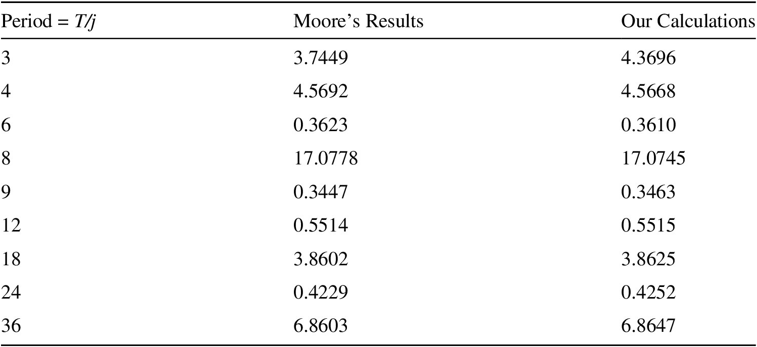
In this section we attempt to replicate Moore’s (Reference Moore1914) calculation of the periodogram for rainfall in the Ohio Valley between 1839 and 1910. The data are given as annual figures in inches with a total of seventy-two observations and can be found in Table I of the appendix to chapter II of Moore (Reference Moore1914, p. 58). First, we calculate the periodogram for the data using the standard method in which the frequencies are defined as  $ {\lambda}_j=2\pi j/T;j=1,...,T/2 $. The results for the amplitude of the cyclical component associated with each frequency are given in Table 1. This allows a direct comparison of our results with those of Moore in cases where
 $ T/j $ is an integer.
Amplitude of the Cyclical Component for Different Periods

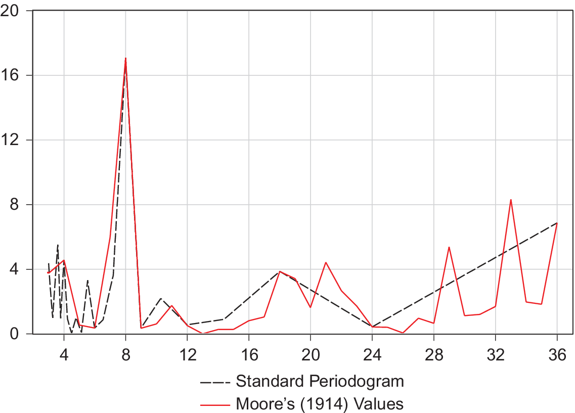
From Table 1, we note that, apart from cycles of period 3, our results are equal to those obtained by Moore (Reference Moore1914) to two decimal places. Some difference is to be expected since Moore was probably using the tables provided by Turner (Reference Turner1913, p. 5), who describes his figures as being accurate “to two figures, which suffice for much of the exploring work represented by Professor Schuster’s periodogram method.” The difference in the figure for cycles of period 3 is much larger, but, given the similarity of all the other figures and the fact that Moore did not have the advantages of electronic computing equipment, it is most likely that this represents an error in his calculations. We therefore conclude from this that we can replicate Moore’s calculations to a fairly high degree of accuracy in cases in which  $ T/j $ is an integer. However, this does not allow us to investigate cases in which this condition fails. This is illustrated in Figure 1, which shows Moore’s periodogram (ch. II, p. 16) with the corresponding amplitudes calculated by the standard method superimposed. Although the two calculations match reasonably well when
 $ T/j $ is an integer, there are numerous cases in which cycles of given length do not correspond to an integer number of cycles during the data period, and this is particularly the case for longer length cycles. A particular problem is that the standard method provides no information that would allow us to identify cycles with length between twenty-four and thirty-six years. This rules out the potentially interesting case of the thirty-three-year cycle identified by Moore.
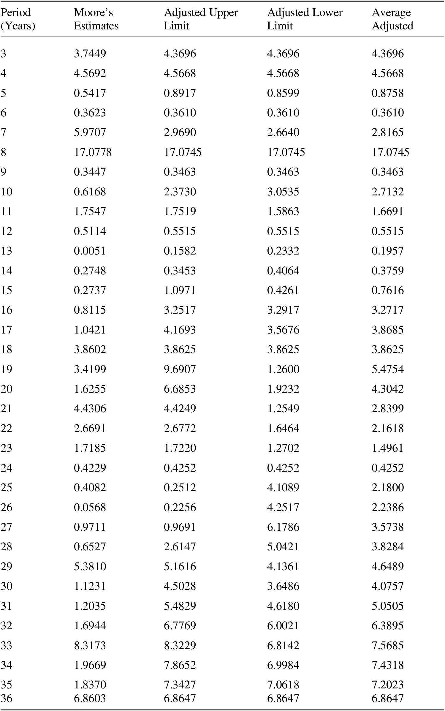
The problem we have in replicating Moore’s analysis is that the summations in (4) and the other orthogonality conditions must take place over a completed set of cycles to be valid. If we fix the period of the cycle and keep the full sample of data, then this will not be the case. Moore must have encountered this problem, but, unfortunately, he does not go into detail about how he addressed it. However, given that the source of the problem is that the full sample does not correspond to a complete set of cycles, a reasonable strategy might be to limit the sample to ensure that this condition is met. For example, to estimate the amplitude corresponding to a thirty-three-year cycle, there is a maximum of two complete cycles in the full sample of seventy-two observations. We could therefore set the data period to 1839 to 1904, which would yield two complete cycles consisting of sixty-six observations. Of course, it would be equally valid to cut the start of the sample and use the data period 1845 to 1910, which would yield an equally valid sample period. We have no idea which, if either, of these approaches Moore took and therefore, in Table 2, we calculate both as well as the average estimate, which has the advantage of using all the data available.
Full Periodogram Alternative Estimates for Amplitude

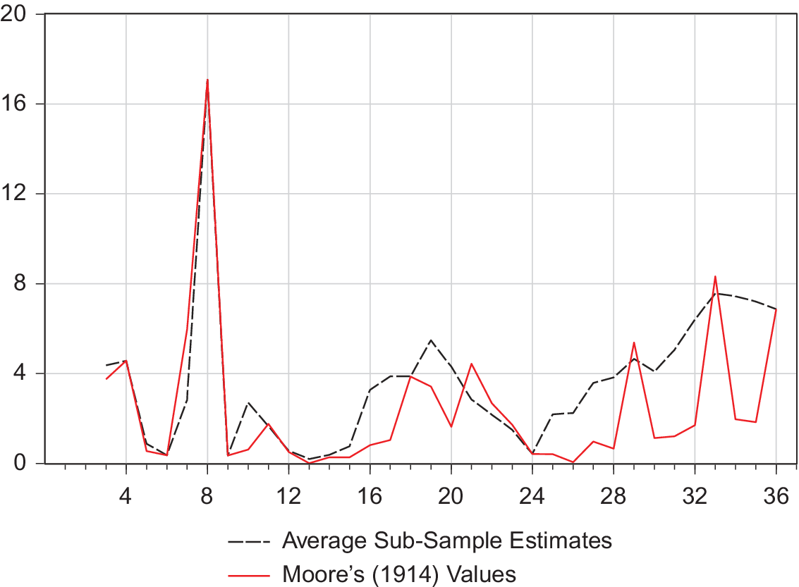
Table 2 indicates that neither of our adjusted sample estimates matches Moore’s estimates particularly closely. The average estimate does have a peak at the thirty-three-year period, as he finds. However, this is not the sharp peak he identifies but, rather, a plateau, as is evident from the plot in Figure 2. Moreover, the peak at thirty-three years is present only in the case where the upper bound of the data is adjusted. When the lower bound is adjusted, then the peak occurs at thirty-four years. The evidence from Table 2 and Figure 2 therefore suggests that Moore did not use simple adjustments of the end-points of the data to calculate amplitudes for cycles with non-integer values of  $ T/j $.
Comparison of Moore’s (Reference Moore1914) Reported Values with Estimates Based on Sub-Samples of Data with Complete Cycles

IV. CONCLUSIONS
In this paper we take issue with Stigler’s (Reference Stigler1962, p. 12) assessment that Moore’s work on cycles should be judged “a complete failure.” From the perspective of 1962, the lack of attention to the demand side of the economy and the link between the economic and rainfall cycles must have looked like a dead end. From a modern perspective, however, the rainfall cycle can be interpreted as the sort of exogenous productivity variation that drives cycles in the real business cycle literature. If Moore had simply identified the cause of the cycle as exogenous changes in rainfall, then he may well have been acclaimed as the father of real business cycle theory.Footnote 13 Unfortunately, his identification of the source of productivity shocks is an astronomical phenomenon in the form of the transits of the planet Venus. Having said that, at least Moore does identify, in the form of the rainfall cycle, a plausible source of productivity shocks, which is more than is the case for many modern real business cycle practitioners.
The failure to recognize Moore’s contribution here lies in his essentially nineteenth-century view of the business cycle as a regular process with fixed period and amplitude, which led him to look for exogenous forcing variables with these characteristics. Le Gall (Reference Le Gall1999) argues that this is a product of his use of periodogram analysis. While this is certainly a contributing factor, it is also true that the vision of the business cycle as a regular process was widespread among economists of the late nineteenth and early twentieth centuries and is not exclusively associated with a particular empirical method. Morgan (Reference Morgan1990, p. 35) also highlights the general belief of economists at the time that business cycles were nothing more than roughly regular: “Critics of Moore’s work were suspicious of the periodicity claimed for the economic cycle, a double claim since it was central to his hypothesis and it implied his usage of the periodogram method.” Morgan states that even if economists believed in periodicity, there was still difficulty in interpreting the results of the periodogram;Footnote 14 furthermore, there were also technical difficulties in the application of the use of periodogram analysis itself, with researchers often finding “chance” or “spurious” periodicities (Morgan Reference Morgan1990, p. 37).
Ultimately, Moore’s place in the history of economic thought depends on his methodological innovations rather than the particular results he presents. Here, we are on stronger ground. Although Fourier analysis has not become the dominant methodology in time series econometrics, there is no doubt that Moore made a significant innovation by being the first to apply it to economic problems. Moreover, he did so in a way that differed from the existing applications to physical phenomena that had characterized the work of physicists such as Schuster and permitted the identification of long-period cycles. Again, the fact that such cycles were ultimately shown to be unimportant does not diminish the contribution of Moore, who deserves to be seen as one of the major innovators of early time series econometrics.