





1. Introduction
When a high-pressure gas sphere is suddenly released into a surrounding compressible fluid, the sphere will expand rapidly and form a shock wave propagating outward. The related shock wave and bubble dynamics have long attracted interest in the fluid-mechanics community. Extensive studies have examined shock formation and material-interface dynamics (Friedman Reference Friedman1961; Holt Reference Holt1977; Kedrinskii Reference Kedrinskii2005; Ling & Balachandar Reference Ling and Balachandar2018; Zhang et al. Reference Zhang, Li, Cui, Li and Liu2023; Matos et al. Reference Matos, Galuska, Javier, Kishore, LeBlanc and Shukla2024). If the surrounding medium is air the problem is commonly called an air blast; if the surrounding medium is water it is referred to as an underwater explosion.
Both scenarios share similar dynamical features, characterised by an inward rarefaction, a material interface and an outward shock (Brode Reference Brode1957). For air blasts, a variety of theoretical approaches exist. Taylor (Reference Taylor1955) and Sedov (Reference Sedov1959) derived self-similar solutions for infinitely intense air blasts, neglecting initial charge size and ambient pressure (suitable for nuclear-scale events). For finite-size charges and finite-duration energy release, spherical-piston models (Taylor Reference Taylor1946; Whitham Reference Whitham1950) give more realistic predictions. However, many of these models neglect the internal gas dynamics and thus cannot capture the inward rarefaction developing into a secondary shock. To address that limitation, Brode and others (Brode Reference Brode1957; Friedman Reference Friedman1961) incorporated the internal gas dynamics of the explosion products, providing formulas for the main and secondary shock fronts and for the interface motion. More recently, Ling & Balachandar (Reference Ling and Balachandar2018) refined these analyses and matched short- and long-time asymptotics for an air blast problem.
Underwater explosions are more complex because water’s higher density and lower compressibility alter wave speeds and energy fluxes. The shock wave from an underwater explosion is often more damaging than its air-blast counterpart because of its higher energy-flux density, and engineering estimates are still often based on empirical formulas such as Cole’s law (Cole Reference Cole1948) or Zamyshlyaev’s far-field correlation. Many theoretical models therefore focus on far-field propagation, where the shock is weak and inward characteristics can be neglected. The well-known Kirkwood–Bethe solution (Kirkwood & Bethe Reference Kirkwood and Bethe1942; Denner Reference Denner2024) predicts the propagation of the quantity
 $\rho u^2 + p$
with a characteristic speed related to
 $u + c$
. Whitham (Reference Whitham1956) analysed shock-profile evolution and energy dissipation, providing methods to predict shock strength and front radius. Rogers (Reference Rogers1977) derived a weak-shock solution for exponentially decaying initial pressure histories, which was then extended to an arbitrary shock profile (Rogers & Weiner Reference Rogers and Weiner1979). These weak-shock approaches neglect entropy production at the shock front (Whitham Reference Whitham1956). When a near-field solver hands off a shock wave to a far-field model at a moderate distance to obtain an efficient prediction of long-range propagation, the shock is too strong to ignore the entropy production at the front. Nevertheless, the predictive methods still lack a framework that simultaneously accounts for entropy production, accommodates arbitrary shock profiles and remains efficient over long propagation distances. Filling that gap is important for connecting near-field shock formation to far-field loading and bubble response.
Numerical simulation of underwater explosions has also advanced substantially. Because viscosity and thermal conduction are usually negligible over the short time scales and high pressures of interest, the Euler equations are commonly used to model the flow field. The principal numerical difficulties are the multiple spatial and temporal scales and the presence of fast-moving discontinuities, namely the shock front and the contact discontinuity at the bubble surface. Eulerian fixed-grid methods therefore require dedicated interface and shock-capturing treatments such as ghost-fluid methods (Liu et al. Reference Liu, Shu and Zhang2021; Shen et al. Reference Shen, Yan, Pei, Jiang, Mao and Yu2024),
 $\gamma$
-based models (Shyue Reference Shyue1998; Kong et al. Reference Kong, Liu, Li, Ma, Hao and Zhang2025; Yu et al. Reference Yu, Zhang, Wang, Hao and Mao2025) or volume-of-fluid methods (Tian et al. Reference Tian, Zhang, Liu and Tao2021). When a strong shock crosses the mesh, non-physical oscillations can easily appear; artificial viscosity and similar treatments may suppress them, but at the cost of smearing the shock front. Lagrangian methods naturally track the bubble interface (Arons Reference Arons1954; Brode Reference Brode1955; Wang et al. Reference Wang, Zhang, Ming, Sun and Cheng2019), but resolving an external moving shock with sufficient sharpness remains difficult. Sufficiently resolved high-fidelity simulations can capture these phenomena with comparable physical fidelity (Wardlaw Jr. & Mair Reference Wardlaw and Mair1998; Ling & Balachandar Reference Ling and Balachandar2018; Jiang et al. Reference Jiang, Tao, Chen and Dai2025). However, such simulations usually require substantially higher computational cost, especially when long-range pressure-wave propagation must also be resolved. To reduce the cost of the direct solution of the Euler equations, linear acoustic approximations are often used once the shock becomes weak enough. Those approaches can predict reflections and cavitation (Sprague & Geers Reference Sprague and Geers2003, Reference Sprague and Geers2006; Wu et al. Reference Wu, Liu, Zhang, Liu and Liu2020; Liu et al. Reference Liu, Hao, Zhong, Chen, Kong and Zhang2025), but they still face difficulties in representing a steep shock profile. Moreover, the wave equation remains almost as stiff as the Euler equations, so long-range propagation can still require prohibitively small time steps.
Besides the shock wave, violent bubble motion is a feature unique to underwater explosions (Cole Reference Cole1948). Oscillations analogous to those in underwater explosions exist in air blasts, but they are typically negligible by comparison (Ling & Balachandar Reference Ling and Balachandar2018). The bubble motion is driven by the large pressure and density contrast across the interface between the explosion products and the surrounding water. In most theoretical bubble-dynamics models (Plesset & Chapman Reference Plesset and Chapman1971; Keller & Miksis Reference Keller and Miksis1980; Zhang et al. Reference Zhang, Li, Cui, Li and Liu2023, Reference Zhang, Li, Xu, Pei, Li and Liu2024), the gas inside the bubble is treated as effectively massless and its pressure is evaluated from an adiabatic equation of state using the instantaneous bubble volume. Internal wave effects are therefore neglected. Geers & Hunter (Reference Geers and Hunter2002) proposed a coupled model that retains internal gas dynamics by separating the motion into uniform expansion and wave components. They used the doubly asymptotic approximation to describe the wave field, leading to the conclusion that internal waves contribute substantially to bubble-energy dissipation. However, because the doubly asymptotic approximation model is linear and heavily simplified, it does not resolve the travelling-wave structure inside the bubble and cannot capture multiple secondary shocks.
To address these difficulties, we develop a unified modelling framework with three related contributions. First, the mapped near-field formulation combines high-order discontinuous Galerkin (DG) discretisation with analytically supplied interface and shock conditions. By fixing the bubble interface and shock front on subdomain boundaries, it avoids the numerical diffusion and spurious oscillations commonly associated with strong discontinuities crossing computational cells. Second, analysis of the inward and outward characteristics of the nonlinear Euler equations yields a far-field pressure-evolution equation that accepts the arbitrary finite-strength profile supplied by the near-field solution. This derivation provides a mathematical connection between nonlinear shock formation and long-range profile evolution while substantially relaxing the Courant–Friedrichs–Lewy (CFL) restriction. Third, resolving the internal gas field reveals the complete pathway by which converging and reflected gas waves transmit through the bubble surface, and a scaling analysis quantifies when these waves affect bubble oscillation and the emitted pressure signal. The internal-wave reflections and secondary shocks themselves are established phenomena; the physical contribution here is their mechanistic and quantitative interpretation within the unified framework. The rest of the paper is organised as follows. Section 2 presents the problem formulation and governing equations. Section 3 introduces the domain partition, coordinate mapping and near-field numerical method. Section 4 derives the far-field model and its numerical implementation. Section 5 examines how internal wave motion affects bubble oscillation and the emitted pressure signal. Finally, § 6 summarises the main conclusions.
2. Problem description and basic equations
Consider the explosion of a spherical charge of radius
 $R_c$
in undisturbed water with ambient state
 $(\rho _0,p_0,c_0)$
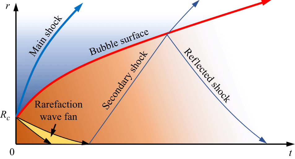
denoting density, pressure and sound speed. The detonation is assumed instantaneous. The problem forms a spherical two-medium Riemann problem: the high-pressure gaseous products are separated from the external fluid by a spherical surface, and the fluid is initially at rest. A shock wave and a rarefaction wave propagate outward and inward, respectively (figure 1).
Sketch for the wave structure of a high-pressure gas bubble released underwater.

We denote the time-dependent locations of the bubble surface (the contact discontinuity between the internal gas and the external fluid) and the shock-wave front as
 $R_b(t)$
and
 $R_s(t)$
, respectively. In this process, viscosity, surface tension and heat conduction are reasonably neglected because the characteristic time scale is short and the pressure level is high (Kadioglu & Sussman Reference Kadioglu and Sussman2008; Matos et al. Reference Matos, Galuska, Javier, Kishore, LeBlanc and Shukla2024; Jiang et al. Reference Jiang, Tao, Chen and Dai2025). If interface instabilities and nearby boundaries that would break spherical symmetry are also neglected, the flow field can be modelled by the one-dimensional Euler equations in spherical coordinates, reading
 \begin{equation} \frac {\partial \boldsymbol{U}}{\partial t} + \frac {\partial \boldsymbol{F}}{\partial r} = \boldsymbol{S} \end{equation}
with
 \begin{align} \boldsymbol{U} = \begin{bmatrix} \rho \\[3pt] \rho u \\[3pt] E \end{bmatrix}\!,\quad \boldsymbol{F} = \begin{bmatrix} \rho u \\[3pt] \rho u^2 + p \\[3pt] u(E+p) \end{bmatrix}\quad \text{and}\quad \boldsymbol{S} = -\frac {2}{r}u\begin{bmatrix} \rho \\[3pt] \rho u \\[3pt] E+p \end{bmatrix} \end{align}
representing the conserved variables, flux and geometrical source terms, respectively. Herein,
 $u$
,
 $\rho$
and
 $p$
are the fluid radial velocity, density and pressure and
 $E = (1/2)\rho u^2+\rho e$
is the total specific energy, with
 $e$
denoting the specific internal energy per unit mass.
An equation of state (EOS) closes the system for each material. For the gaseous explosion products inside the bubble we use the Jones–Wilkins–Lee (JWL) EOS:
 \begin{equation} p=A\left ( 1-\frac {\omega \rho }{{{R}_{1}}{{\rho }_c}} \right )\exp \left ( -\frac {{{\rho }_c}}{\rho }{{R}_{1}} \right )+B\left ( 1-\frac {\omega \rho }{{{R}_{2}}{{\rho }_c}} \right )\exp \left ( -\frac {{{\rho }_{c}}}{\rho }{{R}_{2}} \right )+\omega \rho {{e}}, \end{equation}
where
 $A$
,
 $B$
,
 $R_1$
,
 $R_2$
and
 $\omega$
are material constants of the explosive and
 $\rho _c$
denotes the initial density. When
 $A$
and
 $B$
are both set to 0 and
 $\gamma = \omega + 1$
, the JWL EOS reduces to the ideal-gas equation
 \begin{equation} p = \rho e (\gamma -1), \end{equation}
which can be used to model the expansion and shock-wave formation of compressed air (Friedman Reference Friedman1961; Ling & Balachandar Reference Ling and Balachandar2018). We use the stiffened-gas EOS to describe the water outside the bubble:
 \begin{equation} p=\rho e(\gamma -1)-\gamma {{P}_{w}}, \end{equation}
where
 $\gamma$
and
 $P_w$
are material constants. When
 $P_w=0$
the stiffened-gas EOS reduces to the ideal-gas equation, too, which allows application to air-blast cases. The material constants used in this paper are listed in tables 1 and 2.
The material constants for the JWL equation of TNT explosive.

Table 1. Long description
A table with one row and eight columns listing material constants for the JWL equation of TNT explosive. The columns are labeled as follows: rhoc (kg m-3), A (GPa), B (GPa), R1, R2, omega, and ec (MJ kg-1). The values in the row are: 1630, 371.2, 3.231, 4.15, 0.95, 0.3, and 4.3 respectively.
The material constants for the stiffened-gas equation of water and air.

Table 2. Long description
A table comparing material constants for water and air using the stiffened-gas equation. The table has three columns and two rows. The columns are labeled Material, rho0 (kg m-3), Pu (MPa), and gamma. The row labels are Water and Air. Row 1: Water, 1000, 330.9, 7.5. Row 2: Air, 1.29, 0, 1.4.
3. Near-field shock-wave formation and propagation
3.1. Fluid field partition and transformation in the stretched coordinate system
First, we consider the early stage of shock formation and propagation, during which the full Euler system (2.1) must be resolved because the flow is strongly nonlinear. The main numerical difficulty is the presence of two rapidly moving strong discontinuities, namely the shock front
 $R_s$
and the contact discontinuity at the bubble surface
 $R_b$
. With a fixed Eulerian mesh, both discontinuities require special treatment through interface-tracking or shock-capturing procedures. A Lagrangian method naturally follows the bubble interface, but the external shock front is still not resolved sharply.
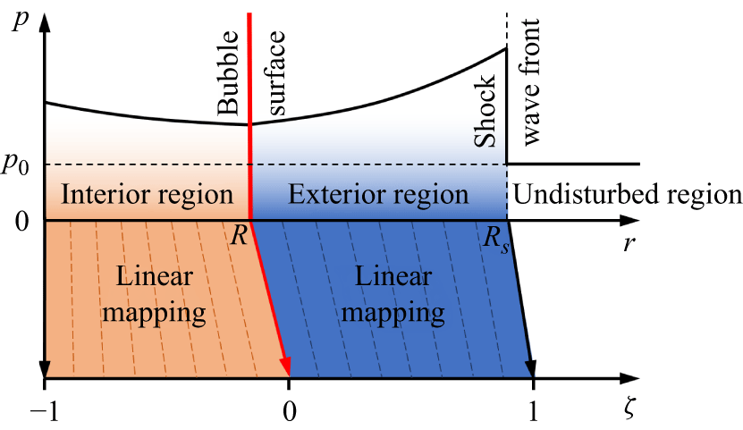
Thus, we solve the hydrodynamics in two stretched coordinate systems based on the idea of the arbitrary Lagrangian–Eulerian method. As shown in figure 2, we partition the whole domain into three regions:
-
(i) interior region inside the underwater explosion bubble, i.e.
 $0\lt r\lt R_b$
;
-
(ii) exterior region between the bubble surface and the shock-wave front, i.e.
$R_b\lt r\lt R_s$
; -
(iii) undisturbed region
$r\gt R_s$
.


In this paper,
 $R_b$
and
 $R_s$
are obtained by explicitly integrating the interface velocity
 $\dot {R}_b$
and the shock-front velocity
 $\dot {R}_s$
, respectively, as described in § 3.3. Obviously, only the first two regions need to be solved. In this way, the two strong discontinuities remain on region boundaries and can be resolved accurately provided that appropriate boundary conditions are supplied. This boundary-aligned treatment is central to the near-field approach: the discontinuities do not sweep through DG cells, so high-order accuracy can be retained in the smooth parts of each subdomain without relying on artificial diffusion to stabilise the shock and material interface.
Linear mapping from physical coordinate
 $r$
to the stretched coordinate
 $\zeta$
.

Now, let us denote
 $L^{(1)} = R_b$
and
 $L^{(2)} = R_s - R_b$
as the lengths of the two regions in physical space. A mapping from the physical coordinate
 $r$
to a stretched coordinate
 $\zeta$
is then introduced so that
 $\zeta (r = 0)$
,
 $\zeta (r=R_b)$
and
 $\zeta (r=R_s)$
remain constant. The computational domains of the interior and exterior regions are therefore fixed in time, and explicit capture or tracking of the moving jumps is avoided. Because the near-field model is used only while the shock remains relatively close to the source, the physical domain is not excessively large; in this regime, a linear mapping is sufficient to resolve the relevant flow features with a moderate number of DG cells, reading
 \begin{equation} \zeta = \begin{cases} (r-R_b)/L^{(1)},\quad \text{for } \quad r\lt R_b, \\[3pt] (r-R_b)/L^{(2)},\quad \text{for } \quad r\gt R_b. \end{cases} \end{equation}
Note that a nonlinear mapping would be preferable if the near-field solver were extended to much larger distances, because it could retain higher resolution near the shock front and the bubble interface. Then, the local velocity
 $\hat {u}$
in the stretching coordinate system
 $\zeta$
can be expressed by
 \begin{align} \hat {u} = \frac {{\rm d} \zeta }{{\rm d} t} = \frac {1}{L^{(i)}}\big(u - \zeta \dot {L}^{(i)}-\dot {R}_b \big), \end{align}
where the superscript
 $(i)$
can take 1 and 2 accordingly. Plugging (3.1) and (3.2) into (2.1), we obtain the Euler equation system in the stretching coordinate system, reading
 \begin{equation} \frac {\hat {\partial } \boldsymbol{U}}{\hat {\partial } t} + \frac {\partial \hat {\boldsymbol{F}}}{\partial \zeta } = \hat {\boldsymbol{S}}, \end{equation}
where
 $\hat {\partial }/\hat {\partial } t$
denotes the derivative with respect to
 $t$
at a fixed
 $\zeta$
and
 \begin{align} \hat {\boldsymbol{F}} = \begin{bmatrix} \rho \hat {u} \\[3pt] \rho u\hat {u}+p/L^{(i)} \\[3pt] \hat {u}E+up/L^{(i)} \end{bmatrix}\!, \quad \hat {\boldsymbol{S}} = -\frac {2}{r}u\begin{bmatrix} \rho \\[3pt] \rho u \\[3pt] E+p \end{bmatrix}-\boldsymbol{U}\frac {\dot {L}^{(i)}}{L^{(i)}}. \end{align}
Note that the above system still uses the same conserved variables as the original Euler equations to ensure a straightforward evaluation. The first source term in
 $\hat {\boldsymbol{S}}$
is the geometrical source term, which is the same as that in (2.1) but with the additional term
 $-\boldsymbol{U}\dot {L}^{(i)}/L^{(i)}$
to account for the change of the Jacobian between the two coordinate systems.
3.2. Discretisation with the Runge–Kutta DG method
In this paper, we adopt the Runge–Kutta DG (RKDG) method to discretise and solve the Euler equation (3.3) for its flexibility in changing the accuracy order (Cockburn et al. Reference Cockburn, Lin and Shu1989, Reference Cockburn, Hou and Shu1990; Liu et al. Reference Liu, Shu and Zhang2021; Zhang et al. Reference Zhang, Li, Cui, Li and Liu2023). Here we briefly review the key idea of the RKDG method to implement the numerical discretisation.
First, we partition the computational zone
 $-1\lt \zeta \lt 1$
into
 $2N$
equally spaced cells. Cell
 $n$
is defined by
 $\zeta _n\lt \zeta \lt \zeta _{n+1}$
, where
 $\zeta _n = (n-1)/N -1$
and
 $n = 1,2,\ldots ,2N$
. Denote
 $P^K$
as the polynomial space to the order
 $K$
defined on cell
 $n$
, and
 $\phi _i (i=1,2,\ldots , K+1)$
as a complete set of the polynomial basis. Then, we approximate the exact solution
 $\boldsymbol{U}$
by the numerical solution
 $\boldsymbol{U}_h = \sum _{\ell =1,K+1} \boldsymbol{a}_\ell (t) \phi _\ell (\zeta )$
and plug it into (3.3). Using integration by parts on the product of (3.3) and the test function
 $\phi _m$
, we obtain the semi-discretised formulation
 \begin{equation} \int _{\zeta _n}^{\zeta _{n+1}} \dot {\boldsymbol{a}}_\ell \phi _\ell \phi _m\, {\rm d}\zeta = \int _{\zeta _n}^{\zeta _{n+1}} \left (\frac {\partial \phi _m}{\partial \zeta } \hat {\boldsymbol{F}} + \phi _m \hat {\boldsymbol{S}}\right )\,{\rm d}\zeta - \left . \phi _m \tilde {\boldsymbol{F}} \right |_{\zeta _n}^{\zeta _{n+1}}, \end{equation}
where
 $\tilde {\boldsymbol{F}}$
denotes the numerical flux. For simplicity, we use the Lax–Friedrichs flux for the interior cell boundaries of each region. The numerical flux calculation for the exterior boundaries of each region is explained in § 3.3 as boundary conditions. Once
 $\dot {\boldsymbol{a}}$
is obtained the solution is advanced in time using a strong-stability-preserving Runge–Kutta method (Gottlieb et al. Reference Gottlieb, Shu and Tadmor2001), and
 $\boldsymbol{U}_h$
is reconstructed from the modal coefficients.
3.3. Boundary conditions
Three boundary conditions must be provided to complete the model. The first is at the explosive centre (
 $r=0$
, i.e.
 $\zeta = -1$
), where the radial velocity must be zero due to symmetry, giving
 \begin{equation} \tilde {\boldsymbol{F}}|_{\zeta = {-1}} = \frac {1}{L^{(1)}}\begin{bmatrix} 0 \\[3pt] p \\[3pt] 0 \end{bmatrix}\!, \end{equation}
where
 $p$
is evaluated from the interior solution at
 $\zeta = -1^+$
with the superscript
 $+$
indicating the limit approaching the boundary from the positive side.
The second condition is at the bubble surface where
 $r =R_b$
, i.e.
 $\zeta = 0$
, given by a two-medium Riemann problem:
 \begin{equation} \begin{cases} (\rho _L,u_L,p_L) = (\rho ,u,p)|_{(0^-,t)}, \\[3pt] (\rho _R,u_R,p_R) = (\rho ,u,p)|_{(0^+,t)}. \end{cases} \end{equation}
Because the primary shock propagates away from the interface there is no strong shock–interface interaction, so a linearised Riemann solver suffices to approximate the interface flux. With the linearised relation
 ${\rm d}p/{\rm d}\rho =c^2$
for both materials, the dynamic pressure balance gives us
 \begin{equation} p_L+(u_L-u^*)\rho _L c_L = p^* = p_R+(u^*-u_R)\rho _R c_R, \end{equation}
where the superscript
 $*$
denotes the intermediate state of the star region. By solving the above equation, we have
 \begin{equation} u^* = \frac {1}{\rho _Lc_L+\rho _Rc_R}(\rho _Lc_Lu_L+\rho _Rc_Ru_R+p_L-p_R), \end{equation}
which is used to update the radius of the bubble, i.e.
 \begin{equation} \dot {R}_b = u^*. \end{equation}
Then, the numerical fluxes for the interior and exterior regions at the bubble interface are given by
 \begin{equation} \tilde {\boldsymbol{F}}|_{\zeta = 0^-} = \frac {1}{L^{(1)}}\begin{bmatrix} 0 \\[3pt] p^* \\[3pt] u^*p^* \end{bmatrix}\quad \text{and}\quad \tilde {\boldsymbol{F}}|_{\zeta = 0^+} = \frac {1}{L^{(2)}}\begin{bmatrix} 0 \\[3pt] p^* \\[3pt] u^*p^* \end{bmatrix}\!, \end{equation}
respectively.
The third condition should be provided at the shock-wave front
 $r = R_s$
where the undisturbed water flows into the computational domain with a speed of
 $\dot {R}_s$
. Speed
 $\dot {R}_s$
can be calculated with the Hugoniot condition (Friedman Reference Friedman1961; Toro Reference Toro2009) of the discontinuity
 \begin{equation} p_s+P_w = \frac {p_0+P_w}{\gamma +1}\left (2\gamma \frac {\dot {R}_s^2}{c_0^2} -\gamma + 1\right ) \end{equation}
provided the shock pressure peak
 $p_s$
at
 $\zeta =1^-$
is known from the RKDG solution. The numerical flux at the shock boundary is set by
 \begin{equation} \tilde {\boldsymbol{F}}|_{\zeta =1} = \frac {1}{L^{(2)}}\begin{bmatrix} -\dot {R}_s \rho _0 \\[5pt] p_0 \\[5pt] -\dot {R}_s\frac {p_0+\gamma P_w}{\gamma -1} \end{bmatrix} \end{equation}
based on the conservation of mass, momentum and energy at the shock-wave front. With the numerical fluxes at the three boundaries of the computational domain given by (3.6), (3.11) and (3.13), respectively, the RKDG formulation can be solved explicitly.
3.4. Initial condition
To complete the numerical approach, suitable initial conditions must be prescribed. At
 $t=0$
, the charge surface separates the explosion products from the surrounding water and therefore defines a two-medium Riemann problem. The initial states on the two sides are
 \begin{equation} \boldsymbol{U}_{\!L} = \begin{bmatrix} \rho _c \\[3pt] 0 \\[3pt] \rho _c e_c \end{bmatrix}\quad \text{and}\quad \boldsymbol{U}_{\!R} = \begin{bmatrix} \rho _0 \\[5pt] 0 \\[5pt] \frac {p_0 + \gamma P_w}{\gamma -1} \end{bmatrix}\!, \end{equation}
where
 $p_0$
and
 $\rho _0$
are the pressure and density of the undisturbed water. However, these states cannot be used directly in the mapped numerical model because the disturbed outer region grows from zero thickness as the shock forms. At the initial instant,
 $L^{(2)} = 0$
, so the exterior computational domain does not yet exist and the simulation cannot be started in that form.
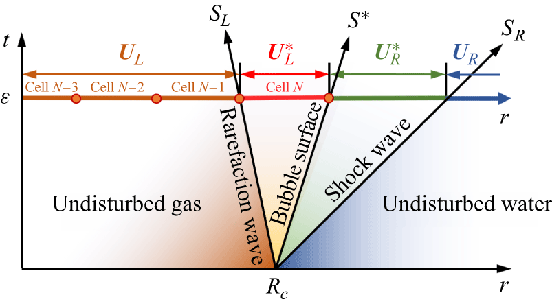
Consider the three-wave HLLC Riemann structure (Toro Reference Toro2009) shown in figure 3. The three signals are the leftward rarefaction
 $S_L$
, the contact discontinuity
 $S^*$
that coincides with the bubble interface and the rightward shock
 $S_R$
representing the primary shock wave. After a short time interval
 $\varepsilon$
, the states separated by these waves are approximately piecewise constant if the rarefaction fan is replaced by a single averaged state. We therefore start the numerical simulation at
 $t=\varepsilon$
rather than at
 $t=0$
. At that instant, the interior region is initialised with the states
 $\boldsymbol{U}_{\!L}$
and
 $\boldsymbol{U}_{\!L}^*$
, while the exterior disturbed region is initialised with
 $\boldsymbol{U}_{\!R}^*$
, as sketched in figure 3.
Assume that the interior region is discretised with
 $N$
DG cells. We assign the state
 $\boldsymbol{U}_{\!L}$
to the
 $M$
cells adjacent to the centre and the state
 $\boldsymbol{U}_{\!L}^*$
to the remaining
 $N-M$
cells near the bubble surface. Then,
 \begin{align} \varepsilon (S^*-S_L) = R_b(\varepsilon )(1-M/N). \end{align}
To keep
 $\varepsilon$
small and thereby minimise the initialisation error introduced by starting from
 $t=\varepsilon$
, we take
 $M=N-1$
, so that the rarefaction spans only one DG cell at the start of the computation. This gives
 \begin{equation} \varepsilon (S^* - S_L) = \frac {R_c + S^*\varepsilon }{N}. \end{equation}
A sensitivity check shows that the solution is insensitive to the precise choice of
 $M$
provided that
 $M$
remains close to
 $N$
. We therefore use this relation to determine
 $\varepsilon$
and initialise the computation.
Based on these assumptions, we construct an approximate two-medium Riemann solver. In the star region between
 $S_L$
and
 $S_R$
, pressure and velocity satisfy
 \begin{equation} \begin{cases} S^* = u^* = u^*_L = u^*_R, \\[3pt] p^* = p^*_L = p^*_R. \end{cases} \end{equation}
Sketch of the approximate Riemann problem used to initialise the computation.

The discontinuity at
 $S_R$
is the primary shock wave, so the Hugoniot condition (Friedman Reference Friedman1961) gives
 \begin{equation} u^* = \frac {2}{\gamma +1}\frac {S_R^2-c_0^2}{S_R}, \end{equation}
where
 $c_0$
is the sound speed of the undisturbed water. Applying the momentum equation to the fluid bulk in
 $\varepsilon S_L\lt r\lt \varepsilon S_R$
, we have
 \begin{equation} u^*=\frac {p_0-p_c}{\rho _cS_L-\rho _0S_R}. \end{equation}
Thus, we have
 \begin{equation} \frac {p_0-p_c}{\rho _cS_L-\rho _0S_R} = \frac {2}{\gamma +1}\frac {S_R^2-c_0^2}{S_R}, \end{equation}
in which
 $S_L$
and
 $S_R$
are unknown. Because
 $S_L$
is a rarefaction fan bounded by its head and tail characteristics, we approximate it by
 \begin{align} S_L \approx -\frac 12 (c_c+c_L^*), \end{align}
namely the arithmetic mean of the sound speeds associated with
 $\boldsymbol{U}_{\!L}$
and
 $\boldsymbol{U}_{\!L}^*$
. With the additional constraint
 $S_R\gt c_0$
, (3.20) then yields a unique value of
 $S_R$
.
The state
 $\boldsymbol{U}_{\!L}^*$
is not known a priori. To close the problem, we express
 $c_L^*$
as a function of
 $p^*$
by assuming that the gas in the left star region is obtained from the initial explosive state through adiabatic expansion. Combined with the Hugoniot relation (3.12), this reduces (3.20) to a nonlinear equation for the single unknown
 $S_R$
.
Once
 $S_R$
is known, (3.12) and (3.18) together with
 \begin{equation} \rho _R^* = \frac {(\gamma +1)\rho _0 S_R^2}{(\gamma -1)S_R^2 + 2c_0^2} \end{equation}
give the corresponding values of
 $u^*$
,
 $p^*$
and
 $\rho _R^*$
. The start-up time
 $\varepsilon$
then follows from (3.16). Using
 $\varepsilon$
, the positions of the bubble surface
 $R_b(\varepsilon )$
and shock front
 $R_s(\varepsilon )$
at
 $t = \varepsilon$
are
 \begin{align} \begin{cases} R_b(\varepsilon ) = R_c + \varepsilon u^*, \\[3pt] R_s(\varepsilon ) = R_c + \varepsilon S_R. \end{cases} \end{align}
For the interior DG cell adjacent to the bubble surface, the density is obtained from mass conservation. Because the gas mass remains constant while the inward rarefaction traverses a single DG cell, we obtain
 \begin{equation} \rho _L^* = \rho _c\frac {R_c}{R_c + N \varepsilon u^*}. \end{equation}
The resulting initial condition used to start the simulation is therefore
 \begin{equation} \boldsymbol{U}(\zeta ,\varepsilon )= \begin{cases} \boldsymbol{U}_{\!L} & \text{for } \quad -1\lt \zeta \lt -\frac {1}{N}, \\[3pt] \boldsymbol{U}_{\!L}^* & \text{for } \quad -\frac {1}{N}\lt \zeta \lt 0, \\[3pt] \boldsymbol{U}_{\!R}^* & \text{for } \quad 0\lt \zeta \lt 1. \end{cases} \end{equation}
3.5. Reduced model with the uniform expansion assumption
The basic idea of this paper was first presented in Zhang et al. (Reference Zhang, Li, Cui, Li and Liu2023), which can be seen as a reduced version of the present model. Here we briefly review and discuss the differences between the two models. We assume that the internal gas expands uniformly and isentropically, so the wave structure inside the bubble is not resolved. The pressure of the internal gas can be expressed as a function of the bubble radius
 $R_b$
:
 \begin{equation} p_g = A \exp \big (\!-(R_b/r_c)^3R_1\big )+B \exp \big (-(R_b/r_c)^3R_2\big ) + C(r_c/R_b)^{\omega +1} \end{equation}
for explosion products, where
 $C$
represents a material constant of the explosive, or
 \begin{equation} p_g = \left (\frac {r_c}{R_b}\right )^{3\gamma } \end{equation}
for ideal gas. Only the exterior region shown in figure 2 then needs to be solved. Compared with the complete model presented in this paper, the scheme is the same, except that the numerical flux at the boundary
 $\zeta = 0$
is expressed as
 \begin{equation} \hat {\boldsymbol{F}}|_{\zeta =0} = \frac {1}{L^{(2)}}\begin{bmatrix} 0 \\[3pt] p_g \\[3pt] \dot {R}_bp_g \end{bmatrix} \end{equation}
with
 $\dot {R}_b = u|_{\zeta = 0}$
.
The uniform expansion assumption is reasonable if the density of the internal gas is sufficiently small so that its sound speed is large and its kinetic energy is negligible. However, the initial density of the internal gas may be of the same order as that of the surrounding water, which can violate this assumption. This assumption becomes more accurate as the bubble expands and the gas density decreases. Accordingly, it has been widely adopted in models for underwater explosion bubble dynamics (Prosperetti & Lezzi Reference Prosperetti and Lezzi1986; Zhang & Liu Reference Zhang and Liu2015; Zhang et al. Reference Zhang, Li, Cui, Li and Liu2023), which typically start from a well-expanded bubble. We compare the results of the two models in § 3.6.
3.6. Validation and analysis
In this section, we validate and analyse the model using a representative underwater explosion case with a 7 kg TNT charge. The pressure history is compared with experimental measurements at a stand-off distance of 4.0 m, and the same case is used for the model comparisons below. In the simulations, both the interior and exterior regions are discretised using
 $N$
DG cells with polynomial order
 $K=2$
. A grid-convergence study is carried out with
 $N=25$
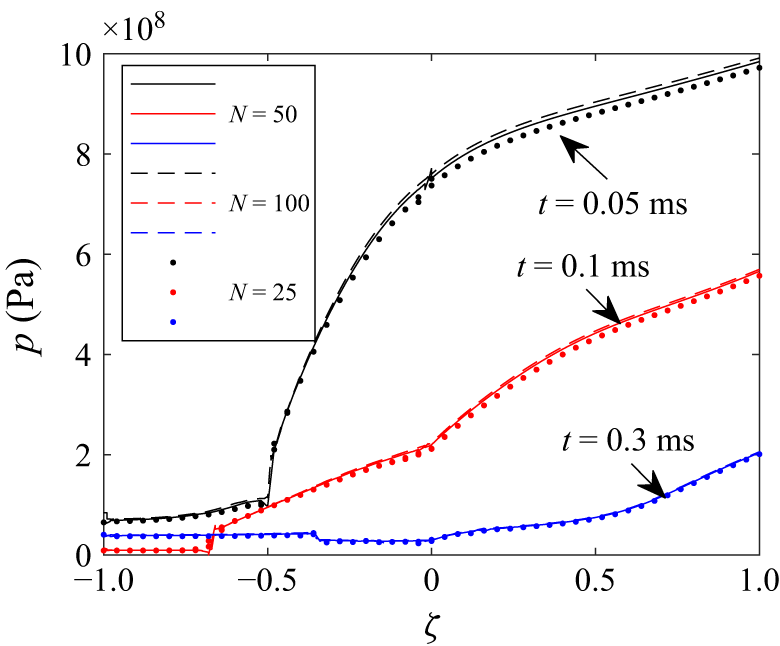
, 50 and 100. Figure 4 compares the pressure distributions along
 $\zeta$
at
 $t = 0.05$
, 0.1 and 0.3 ms. Even
 $N=25$
gives a reasonable solution due to the high-order DG discretisation and the dynamic coordinate mapping, and the results are effectively converged by
 $N=100$
. We therefore use
 $N=100$
in the following calculations.
Grid-convergence analysis for the 7.0 kg TNT underwater explosion case. Pressure distributions along
 $\zeta$
at
 $t = 0.05$
, 0.1 and 0.3 ms are compared for different numbers of DG cells
 $N$
. Pressure is evaluated at cell boundaries to show the discontinuities clearly.

Figure 5 compares the
 $r$
–
 $t$
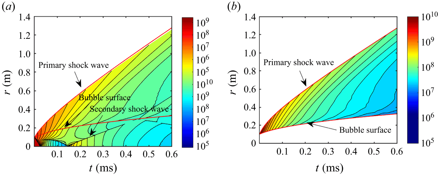
evolution predicted by the present model and by the reduced model of Zhang et al. (Reference Zhang, Li, Cui, Li and Liu2023). In both models, the primary shock originates at the bubble surface and propagates outward while gradually decelerating. Because the present model resolves the gas motion inside the bubble, it also shows the tail of the internal rarefaction steepening into an inward-moving shock. Geometric convergence amplifies this wave as it travels towards the centre, where it reflects and becomes an outward-moving shock that later transmits through the bubble surface to form the secondary shock in water. The reduced model cannot represent this sequence because it does not resolve internal wave motion. Consequently, it predicts the primary shock correctly but misses the secondary shock. The two approaches, however, give very similar bubble-surface trajectories.
Flow-field evolution for the 7.0 kg TNT underwater explosion case predicted by (a) the present model and (b) the reduced model of Zhang et al. (Reference Zhang, Li, Cui, Li and Liu2023). The red curves denote the primary-shock trajectory and the bubble surface.

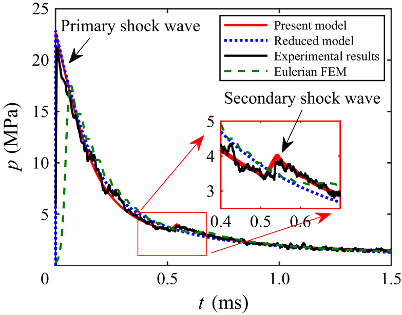
Comparison of simulated and experimental pressure profiles for a 7.0 kg TNT underwater explosion at a stand-off distance of 4.0 m. The zoomed-in view shows the detail of the secondary shock wave.

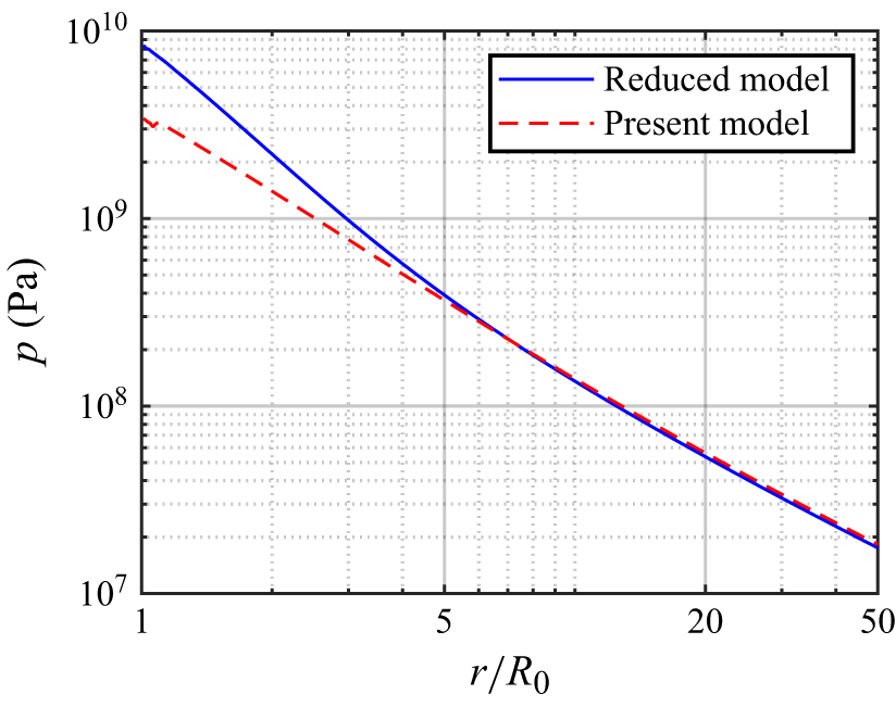
Figure 6 compares the pressure histories predicted by both models at a stand-off distance of 4 m with experimental measurements. Both the present and the reduced approaches reproduce the primary-shock peak reasonably well, but only the present model captures the amplitude and arrival time of the secondary shock. Results from an Eulerian finite-element simulation (Liu et al. Reference Liu, Zhang, Tian and Wang2018) are also shown as a high-resolution conventional benchmark with a fixed mesh. A sufficiently resolved high-fidelity calculation can reproduce the same wave sequence; the comparison instead illustrates the resolution required to obtain a sharp near-field waveform with a fixed mesh. The mapped formulation is designed to reduce this requirement by keeping the principal discontinuities on subdomain boundaries, while its far-field equation avoids continuing the full Euler calculation over long distances. The present Eulerian approach smears the shock front, yielding a main shock peak lower than expected due to numerical viscosity in the shock-capturing scheme. Furthermore, it fails to resolve the secondary shock wave even when using 5000 elements in the radial direction, which is much more computationally expensive than the present approach. At larger distances, the difference between the present and reduced models becomes small because the radiated shock depends mainly on the total released energy (Ling & Balachandar Reference Ling and Balachandar2018). This trend is quantified in figure 7: the reduced model overpredicts the near-field peak pressure, whereas the two models agree closely once
 $r/R_0 \gtrsim 5$
. The complete model is therefore needed for early-time and near-field dynamics, while the reduced model remains useful after the bubble has expanded and internal wave effects have weakened.
Comparison of simulated pressure peaks changing with distance from the present model and the reduced model for the same case as figure 6.

4. Far-field shock-wave evolution
4.1. Equation for the shock-wave evolution with less CFL restriction
Far-field shock-wave evolution is often of interest in engineering applications. Theoretically, the previously described method can be directly applied to simulate the entire propagation process of the shock wave from near field to far field. However, for practical applications, it is usually impractical for two main reasons. First, the physical domain required for simulation would become excessively large, while the shock-wave length remains nearly constant. Consequently, the number of elements would need to increase proportionally with the size of the domain, leading to a significant rise in computational cost. Second, the CFL condition, constrained by both outward and inward characteristics, would demand an unfeasibly large number of time steps to resolve the whole process accurately. Therefore, an alternative approach is necessary to reduce computational cost while preserving accuracy in simulating far-field shock-wave evolution.
We first write the characteristic equations (Shapiro Reference Shapiro1954; Friedman Reference Friedman1961) of (2.1) with pressure and velocity as primary variables:
 \begin{equation} \frac {{\rm d}p}{{\rm d}t} + \rho c \frac {{\rm d}u}{{\rm d}t} = -\frac {2\rho c^2u}{r} \end{equation}
along the outward-propagating characteristics
 ${\rm d}r/{\rm d}t = u+c$
, and
 \begin{equation} \frac {{\rm d}p}{{\rm d}t} - \rho c \frac {{\rm d}u}{{\rm d}t} = -\frac {2\rho c^2u}{r} \end{equation}
along the inward-propagating characteristics
 ${\rm d}r/{\rm d}t = u-c$
. They are valid whether or not the flow is isentropic.
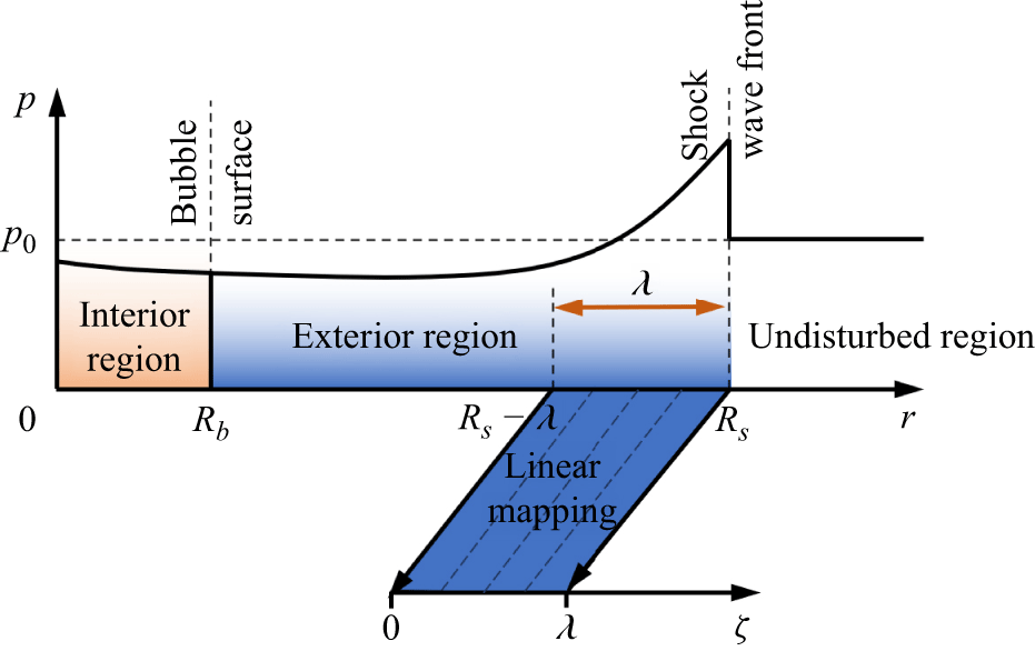
Linear mapping from physical coordinate
 $r$
to the stretched coordinate
 $\zeta$
.

We consider only the fluid domain
 $R_s - \lambda \lt r \lt R_s$
, where
 $\lambda$
denotes a representative shock thickness. This interval is mapped from physical space to a moving coordinate
 $0\lt \zeta \lt \lambda$
by setting
 $\zeta = r - R_s + \lambda$
. In this way, the computational domain remains fixed even though the shock continues to propagate outward. Thus, the characteristic speeds in the moving coordinate system can be written as
 $v$
and
 $v-2c$
, where
 $v=u+c-\dot {R}_s$
, as shown in figure 8. Then, we can rewrite the characteristic equations in the moving coordinate system as
 \begin{equation} \frac {\hat {\partial }p}{\hat {\partial }t} + \rho c \frac {\hat {\partial }u}{\hat {\partial }t} + v \left (\frac {\partial p}{\partial \zeta }+ \rho c \frac {\partial u}{\partial \zeta }\right ) = -\frac {2\rho c^2u}{r} \end{equation}
and
 \begin{equation} \frac {\hat {\partial }p}{\hat {\partial }t} - \rho c \frac {\hat {\partial }u}{\hat {\partial }t} + (v-2c) \left (\frac {\partial p}{\partial \zeta }- \rho c \frac {\partial u}{\partial \zeta }\right ) = -\frac {2\rho c^2u}{r}. \end{equation}
Adding the above two equations together to eliminate
 ${\hat {\partial }u}/{\hat {\partial }t}$
, we have
 \begin{equation} \frac {\hat {\partial }p}{\hat {\partial }t} + (v-c) \frac {\partial p}{\partial \zeta } + \rho c^2 \frac {\partial u}{\partial \zeta } = -\frac {2\rho c^2u}{r}. \end{equation}
Equation (4.4) shows that the first two terms on the left-hand side, which involve the time derivatives of pressure and velocity in the moving frame, are small compared with the terms multiplied by
 $c$
. This means that the shock profile evolves slowly in the moving coordinate system. Neglecting those smaller terms gives the following ordinary differential equation for
 $u$
as a function of
 $\zeta$
:
 \begin{equation} \frac {\partial u}{\partial \zeta }=\frac {1}{\rho c}\frac {\partial p}{\partial \zeta }+\frac {u}{r}\frac {2c}{v-2c}. \end{equation}
Plugging it into (4.5), we arrive at the following equation for the shock-wave evolution in the far field:
 \begin{equation} \frac {\hat {\partial }p}{\hat {\partial }t} + v\frac {\partial p}{\partial \zeta } = -\frac {2\rho c^2u}{r} \left (1 + \frac {c}{v-2c}\right )\!. \end{equation}
Once we determine
 $\rho$
,
 $c$
and
 $u$
as functions of
 $p$
, the above equation can be solved with the RKDG method described in § 3.2 and proper boundary conditions. In the present framework, shock decay is represented primarily through geometric spreading, entropy production at the shock front through the Hugoniot relation and the gradual nonlinear reshaping of the profile in the moving-frame transport equation. Viscous diffusion is not included because it is much weaker than these mechanisms over the propagation range considered here. Equation (4.7) is therefore not an independent empirical far-field closure. It inherits the finite-strength pressure profile and shock-front state from the near-field solution, while the characteristic analysis specifies how that profile evolves after the transition. This establishes the theoretical connection between the two propagation regimes.
Compared with the original pair of characteristic equations, the governing transport speed is reduced from
 $|v-2c|$
to the much smaller quantity
 $|v|$
. The far-field equation is therefore substantially less restrictive from a CFL standpoint and can be integrated with much larger time steps.
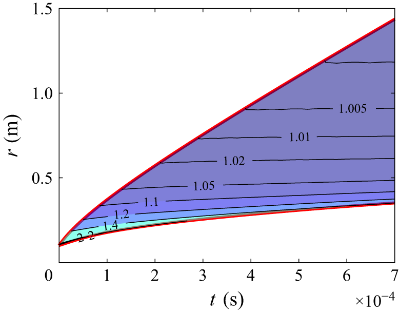
Distribution of the non-dimensional entropy
 $s/s_0$
for the same case as figure 6.

To close the far-field model, we determine
 $\rho$
,
 $c$
and
 $u$
as functions of
 $p$
. Behind the shock front the flow is approximately isentropic, so the entropy is materially conserved:
 \begin{equation} \frac {\hat {\partial }s}{\hat {\partial }t} + (u-\dot {R}_s)\frac {\partial s}{\partial \zeta } = 0, \end{equation}
where
 $s = (p+P_w)/\rho ^\gamma$
is the physical entropy of the fluid. Because
 $|u-\dot {R}_s|$
is large, the entropy varies only weakly across the profile and we simplify the above relation to
 \begin{equation} \frac {\partial s}{\partial \zeta } \approx 0. \end{equation}
Figure 9 supports this approximation for the same case used in figure 6: away from the immediate release region, the entropy is nearly uniform across the far-field shock profile at a given time. Density
 $\rho$
can therefore be obtained from the isentropic stiffened-gas relation (Cole Reference Cole1948)
 \begin{equation} \tilde {p} =\frac {\rho _0^*c_0^{*2}}{\gamma }\left (\frac {\rho }{\rho _0^*}\right )^\gamma - P_w - p_0, \end{equation}
where
 $\tilde {p} = p - p_0$
is the over-pressure of the shock wave and
 \begin{align} \rho _0^* = \left (\frac {p_0+P_w}{s_s}\right )^{ {1}/{\gamma }} \end{align}
is the reference density when the fluid is at the ambient pressure
 $p_0$
and the same entropy as the shock-wave front
 $s_s$
, i.e.
 \begin{align} s_s = \frac {p_s+P_w}{\rho _s^\gamma } \end{align}
with
 $\rho _s$
being the density at the shock-wave front. The sound velocity
 $c$
can be expressed as
 \begin{equation} c = c_0^*\left (\frac {\rho }{\rho _0^*}\right )^{ ({\gamma -1})/{2}}. \end{equation}
To obtain the fluid velocity
 $u$
, we further simplify (4.6) using the far-field condition
 $2c \gg v$
:
 \begin{equation} \frac {\partial u}{\partial r} = \frac {1}{\rho c}\frac {\partial \tilde {p}}{\partial r } - \frac {u}{r}. \end{equation}
Its solution can be written as
 \begin{align} u(r) &= \frac {1}{r}\int _{R_s}^{r} \frac {\eta }{\rho c}\frac {\partial \tilde {p}}{\partial \eta }\,{\rm d}\eta + \frac {R_s}{r}u_s \\[-12pt]\nonumber \end{align}
 \begin{align} & = \mathcal{U}(\tilde {p}) -\frac {R_s}{r}\mathcal{U}(P_m) - \frac {1}{r}\int _{R_s}^r \mathcal{U}(\tilde {p})\,{\rm d}\eta + \frac {R_s}{r}u_s. \end{align}
Here,
 $u_s$
is the material velocity of the shock-wave front,
 $P_m = p_s-p_0$
is the over-pressure peak of the shock wave and
 $\mathcal{U}$
is the acoustic velocity defined by
 \begin{equation} \mathcal{U}(\tilde {p}) = \int _{p_0}^{p_0+\tilde {p}}\frac {{\rm d}p}{\rho c} = \frac {2c_0^*}{{\gamma - 1}}\left [ {{{\left ( {\frac {\tilde {p}}{\rho _0^* c_0^{*2}}\gamma + 1} \right )}^{ ({{\gamma - 1}})/{{2\gamma }}}} - 1} \right ]\!, \end{equation}
where the integration follows the isentropic path.
Another approach to obtain the acoustic velocity is to use the early-stage approximation (ESA) proposed by Geers (Reference Geers1978), reading
 \begin{equation} \rho _0 c_0 u = \tilde {p} + \frac {1}{r} c_0\int _0^t \tilde {p}\, {\rm d}t. \end{equation}
At a given time, the integration in time can be approximated by the integration in space with
 ${\rm d}t = {\rm d}r/c_0$
and the reference state chosen at
 $r = R_s^-$
such that
 \begin{equation} u(r) = u_s + \frac {1}{\rho _0 c_0} \left (\tilde {p}-p_m - \frac {1}{r} \int _r^{R_s} (\tilde {p}-p_m)\, {\rm d}r'\right )\!. \end{equation}
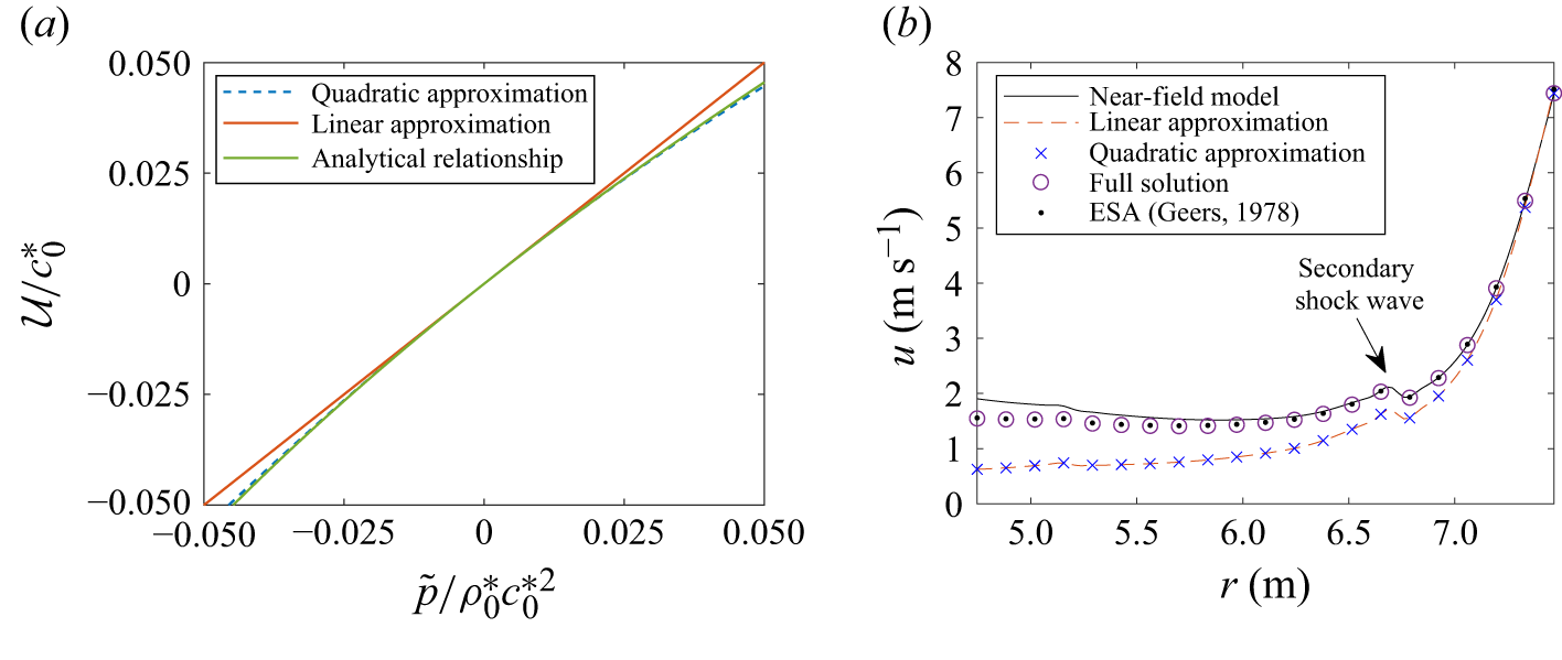
Figure 10(b) compares the velocity obtained from the full solution (4.15), the quadratic approximation (4.21), the linear approximation
 $u = (\rho _0c_0)^{-1}\tilde {p}$
and the ESA against the near-field reference solution for the same explosion case. All four estimates are close near the shock front, but the linear and quadratic approximations deviate as one moves deeper into the profile. The full solution and the ESA agree well with the reference result. We therefore use those forms when an accurate estimate of the local velocity is required; the simpler linear and quadratic approximations neglect geometric spreading and consequently underestimate
 $u$
.
The far-field pressure evolution is therefore obtained by solving (4.7) together with the constitutive relations (4.10), (4.13) and (4.15). The same RKDG framework used in the near-field solver is employed here.
4.2. Conserving form of the shock-wave evolution
Next, we rewrite (4.7) in conservative form to clarify how the shock profile evolves. Expanding
 $1/(\rho c)$
about
 $1/(\rho _0^* c_0^*)$
under the assumption that
 $\tilde {p}/(\rho _0^* c_0^{*2})$
is small gives
 \begin{equation} \frac {1}{\rho c} = \frac {1}{\rho _0^* c_0^*} - \frac {1+\gamma }{2} \frac {\tilde {p}}{\rho _0^{*2} c_0^{*3}}+ O\left (\frac {\tilde {p}}{\rho _0^* c_0^{*2}}\right )^2. \end{equation}
This yields the quadratic approximation
 \begin{equation} \mathcal{U} \approx \frac {\tilde {p}}{\rho _0^* c_0^*}\left (1-\frac {1+\gamma }{4\rho _0^* c_0^{*2}}\tilde {p}\right )\!. \end{equation}
Figure 10(a) compares the linear and quadratic approximations with the analytical expression for
 $\mathcal{U}$
. The quadratic approximation remains accurate up to
 $\tilde {p} = 0.05\rho _0^*c_0^{*2}$
, with a relative error of about 2 %, corresponding to roughly 100 MPa in water.
Comparison of the material velocity calculated from different methods. (a) The linear and quadratic acoustic approximations ignoring the geometric dispersion effect. (b) The shock-wave material velocity of the same case as figure 5.

When the shock radius is much larger than the shock thickness,
 $R_s \gg \lambda$
, substitution of the quadratic approximation for
 $\mathcal{U}$
into (4.17) further simplifies the local velocity to
 \begin{equation} u(\tilde {p}) \approx \frac {\tilde {p}-P_m}{\rho _0 c_0} -\frac 14\frac {\tilde {p}^2-P_m^2}{\rho _0^2 c_0^3}(1+\gamma ) + u_s, \end{equation}
where
 $P_m = p_s - p_0$
is the over-pressure peak of the shock wave. With the above approximation, we can rewrite the convection velocity
 $v$
of the shock-wave profile as
 \begin{equation} v = u+c - \dot {R}_s \approx K_1 + K_2 \tilde {p} + K_3 \tilde {p}^2, \end{equation}
where
 \begin{equation} \begin{cases} K_1= u_s + c_0 - \dot {R}_s - \frac {P_m}{\rho _0 c_0}\left (1 - \frac {1+\gamma }{4 }\frac {P_m}{\rho _0c_0^2}\right )\!, \\[11pt] K_2 = \frac {1}{\rho _0 c_0} \frac {\gamma +1}{2}, \\[11pt] K_3 = -\frac {1+\gamma }{4} \frac {1}{\rho _0^2 c_0^3}. \end{cases} \end{equation}
Substituting (4.23) into (4.7) yields the conservative form
 \begin{equation} \frac {\hat {\partial }\tilde {p}}{\hat {\partial }t} + \frac {\partial }{\partial \zeta } \left(K_1 \tilde {p} + \frac 12 K_2 \tilde {p}^2 + \frac {1}{3}K_3 \tilde {p}^3\right) = -\frac {2\rho c^2u}{r} \left (1 + \frac {c}{v-2c}\right )\!. \end{equation}
This equation resembles a nonlinear transport equation for the shock profile. The first flux term represents linear convection, the higher-order flux terms describe waveform steepening due to the nonlinearity of the water EOS and the right-hand side accounts for geometric spreading together with the leading nonlinear correction.
Now let us compare the above equation with the far-field shock-wave evolution equation proposed by Zhang et al. (Reference Zhang, Li, Cui, Li and Liu2023), which reads
 \begin{equation} \frac {\hat {\partial }\tilde {p}}{\hat {\partial }t} + \frac {\partial }{\partial \zeta } \left ((c_0-\dot {R}_s) \tilde {p} + \frac 34 K_c \tilde {p}^2\right ) = -(c_0+K_c \tilde {p})\frac {\tilde {p}}{r}, \end{equation}
where
 $K_c = ( 1/2)( ({\gamma -1})/{\rho _0 c_0})$
. The present formulation retains a more accurate nonlinear flux and source term by including higher-order pressure effects and the entropy increase generated at the shock front.
4.3. Initial and boundary conditions
Under the far-field assumption, the interaction between the shock wave and the bubble surface is neglected, and the shock wave propagates outward stably. Thus, we require the shock-wave front to be sufficiently far from the bubble surface, and the shock wave to be sufficiently weak, when the far-field model takes over from the near-field model. We define
 $t_c$
as the transition time, at which the far-field model is initialised using the near-field solution. In this paper, we determine
 $t_c$
by the condition
 \begin{equation} \frac {R_s(t_c)}{R_b(t_c)} \gt k, \end{equation}
where
 $k$
is a large enough constant. To evaluate the influence of
 $k$
on the results, we choose
 $k = 5$
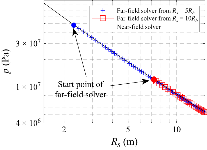
and 10 in the numerical tests and compare the evolution of the shock-wave pressure peak with the near-field model, as shown in figure 11. The results show that the shock-wave pressure peak is not sensitive to the choice of
 $k$
as long as it is large enough. In the present paper, we choose
 $k = 10$
.
Comparison of the shock-wave pressure-peak evolution from the far-field model starting from different initial points with those from the near-field model for the same case as figure 6.

For the choice of
 $\lambda$
, we require the convection velocity of (4.7) to be negative so that the numerical flux at the left boundary of the computational domain is independent of the values at the exterior side due to the upwind principle, i.e.
 \begin{equation} v = u+c - \dot {R}_s \lt 0 \quad \text{at } \quad \zeta = 0. \end{equation}
In this paper, we can choose
 $\lambda = 5 \lambda _0$
, where
 $\lambda _0$
is the shock-wave length at the initial time
 $t_c$
such that
 $v|_{\zeta = \lambda _0} = 0$
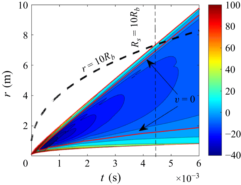
searching from the shock-wave front. As an example, we plot the convection velocity
 $v$
in the
 $t{-}r$
diagram of the underwater explosion case in figure 12. The iso-line of
 $v = 0$
is drawn, which shows that the condition of (4.28) holds for the entire shock-wave propagation process.


Then, the boundary conditions at both ends of the computational domain can be given by the following numerical fluxes:
 \begin{equation} \begin{cases} \hat {F}|_{\zeta = 0} &= F|_{\zeta = 0^+},\\[3pt] \hat {F}|_{\zeta = \lambda } &= F|_{\zeta = \lambda ^-}, \end{cases} \end{equation}
with the shock-wave speed
 $\dot {R}_s$
calculated with (3.12).
4.4. Evolution of shock-wave profile
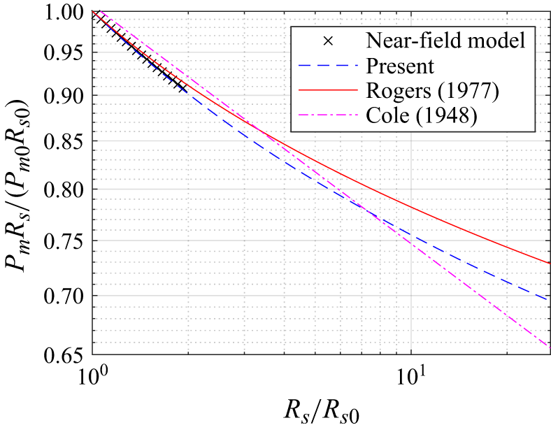
In this section, we compare the results of the present model with others, including the near-field model, the energy-based model (Zhang et al. Reference Zhang, Li, Cui, Li and Liu2023) and the kinetic model (Rogers Reference Rogers1977). The case is still chosen as the same underwater explosion described before in the near-field model. We compare the pressure peak evolution with the distance from the explosive charge in figure 13. The results are given as
 $P_mR_s/(P_{m0}R_{s0})$
, which amplifies the divergence of the decay rates. As a comparison, the results from the near-field model and the decay rate of
 $R_s^{-1.13}$
from Cole (Reference Cole1948) are given as references. We can see that the Rogers model underestimates the decay rate, which has already been stated by comparison with experimental results (Rogers Reference Rogers1977) and attributed to neglecting viscous effects. The present far-field model matches the near-field model well. It also neglects viscous effects and sits between the Rogers model and Cole’s scaling law when
 $R_s$
is large enough, which suggests that the weak-shock assumption in the Rogers model contributes to the discrepancy. Viscous effects may be included in the model in the future to provide closer agreement with experiments.
Comparison of pressure peaks changing with distance calculated from different methods. The case is chosen as the same underwater explosion as in the near-field model. The different models start from
 $R_{s0} = 7.48$
m which satisfies (4.27).

5. Internal wave effect on the bubble oscillation
The internal wave effect not only generates a secondary shock wave, but also influences bubble dynamics through wave–interface interaction. Specifically, the shock wave generated by an underwater explosion reflects at the bubble surface and produces inward-propagating waves that interact with the bubble interior. Geers & Hunter (Reference Geers and Hunter2002) showed that this effect can cause significant energy loss and reduce the maximum bubble radius. In this section, we investigate the internal wave effect on bubble oscillation using the present high-resolution near-field model. Following the non-dimensionalisation method commonly used in bubble dynamics, the characteristic length, density and pressure are chosen as the maximum bubble radius
 $R_m$
, the undisturbed water density
 $\rho _0$
and the hydrostatic pressure
 $p_0$
, respectively (Klaseboer et al. Reference Klaseboer, Hung, Wang and Khoo2005; Zhang & Liu Reference Zhang and Liu2015). Thus, the characteristic velocity and time scales are
 \begin{equation} u' = \sqrt {\frac {p_0}{\rho _0}}, \quad t' = R_m\sqrt {\frac {\rho _0}{p_0}}, \end{equation}
respectively. Here, the maximum bubble radius
 $R_m$
is estimated using the empirical formula of Cole (Reference Cole1948), i.e.
 \begin{equation} R_m = K_C\left (\frac {W}{p_0}\right )^{1/3}, \end{equation}
where
 $W$
is the explosive weight and
 $K_C$
is an empirical constant associated with explosive type, with
 $K_C=72.3\,\mathrm{m}^{1/3}$
for TNT when all variables are in SI units. Another important parameter is the sound speed of the internal gas, which can be estimated using the adiabatic ideal-gas relation. This is a reasonable simplification because the power terms in the JWL equation are negligible during most of the bubble oscillation. Thus, we have
 \begin{equation} c_g \approx \sqrt {\gamma \frac {\bar {p}_g}{\bar {\rho }_g}} = \sqrt {\gamma \frac {p_c( {R_c}/{R_b})^{3\gamma }}{\frac {W}{ (4/3) \pi R_b^3}}}= C_g \left (\frac {W}{R_b^3}\right )^{\tfrac{1}{2} (\gamma -1)}, \end{equation}
where
 $\bar {p}_g$
and
 $\bar {\rho }_g$
are the average pressure and density of the internal gas, respectively, and
 $p_c$
is the characteristic pressure of the explosive, which is taken as 1045 MPa following Geers & Hunter (Reference Geers and Hunter2002). In the last equality we have used
 $R_c=(3W/4\pi \rho _c)^{1/3}$
for a fixed explosive density
 $\rho _c$
, so that
 \begin{align} C_g = \sqrt {\gamma \frac {p_c}{\rho _c^\gamma }\left (\frac {3}{4\pi }\right )^{\gamma -1}} \end{align}
is a material constant. Then, the dimensionless travel time of an internal wave from the bubble surface to the centre, evaluated at
 $R_b=R_m$
, can be written as
 \begin{equation} \gamma _t = \frac {R_m}{c_g t'} = \frac {K_C^{ ({3}/{2})(\gamma -1)}}{C_g \rho _0^{1/2}}p_0^{1-\gamma /2}\approx 8.94 \times 10^{-4}p_0^{1-\gamma /2}. \end{equation}
Note that
 $\gamma _t$
is independent of the explosive weight
 $W$
and the maximum bubble radius
 $R_m$
, but only on the ambient pressure and density of the surrounding water. Thus,
 $\gamma _t$
compares the internal-wave transit time directly with the bubble-oscillation time and provides a physical criterion for whether the internal wave effects can be neglected during the bubble motion.
For illustration, we consider a deep-water explosion with
 $W = 1$
kg and
 $H = 5000$
m, which gives
 $\gamma _t = 0.44$
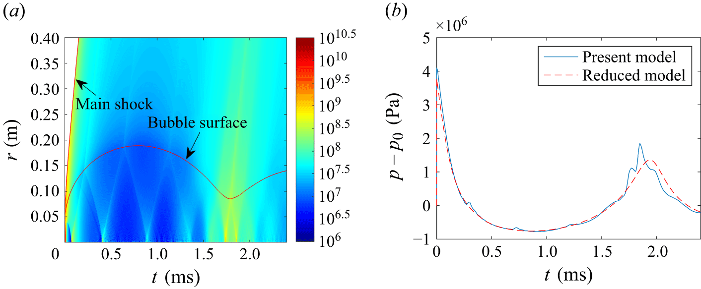
. The time evolution of the pressure field and wave structure inside the bubble is shown in figure 14(a). The internal wave reflects repeatedly within the bubble and each reflection generates a transmitted disturbance in the surrounding water when it reaches the bubble surface. This analysis is intended to quantify the strength and consequences of a known mechanism, rather than to assert that internal wave reflections are newly discovered. Figure 14(b) shows the pressure history at a distance of 10 m from the bubble centre and compares it with the reduced model that neglects internal wave motion. The transmitted waves produce multiple pressure fluctuations, especially during bubble collapse, indicating that internal wave dynamics can materially affect the emitted pressure signal and the bubble oscillation.
The internal wave effect on the bubble oscillation of a deep-water explosion with
 $W = 1$
kg and
 $H = 5000$
m. (a) The pressure field and wave structure inside the bubble. (b) The pressure history at a distance of 10 m from the bubble centre compared with the results from the reduced model without the internal wave effect.

When
 $p_0$
and
 $\gamma _t$
are small, the internal wave effect becomes weak for two reasons. First, the internal wave travels so quickly that successive wave packets overlap and the pressure inside the bubble remains nearly uniform. Second, each transmission through the bubble surface removes wave energy from the bubble. When
 $\gamma _t$
is small, many such reflections occur during the early expansion stage, so the remaining wave energy is too small to influence the later bubble pulsation appreciably.
6. Conclusion
We developed a two-part modelling strategy for spherical underwater explosions that couples a mapped, high-resolution near-field solver with an efficient far-field transport equation for the outgoing shock. The near-field solver advances the Euler equations in two moving subdomains so that the bubble interface and shock front remain on fixed cell boundaries, and the initial singular stage is handled through an approximate two-medium Riemann initialisation.
For propagation at large radii, we derived a reduced evolution equation by eliminating the fast inward characteristic and using the near-isentropic structure behind the front. The resulting transport equation has substantially smaller characteristic speeds, which relaxes the CFL restriction and enables economical time-marching to distances where full-domain simulations would be costly.
Comparisons with benchmark calculations and experimental data show that the coupled approach captures both primary and secondary shocks and reproduces shock-decay trends consistent with full near-field simulations and established empirical scalings. Although sufficiently resolved high-fidelity simulations can also capture these established phenomena, the mapped formulation reduces the fixed-mesh resolution burden for near-field waveform calculation and remains efficient for long-range propagation through the reduced far-field equation. Finally, we quantified the effect of internal wave motion on the bubble pulsation pressure and found that it becomes increasingly important as ambient pressure rises, making it particularly relevant for deep-water explosions.
Future work will focus on interface instability during bubble collapse and the associated energy-loss mechanisms. Another important direction is a detailed scaling analysis of near-field shock formation in deep water.
Funding
The authors acknowledge support from the National Natural Science Foundation of China (NSFC) under grant number 52525102.
Declaration of interests
The authors report no conflict of interest.


 r
 ζ
 ζ
 t=0.05
 N
 r
 ζ
 s/s0
 v
 t−r
 v=0
 r=10Rb
 Rs0=7.48
 W=1
 H=5000

 Open access

