



%20--%3e%3c!DOCTYPE%20svg%20PUBLIC%20'-//W3C//DTD%20SVG%201.0//EN'%20'http://www.w3.org/TR/2001/REC-SVG-20010904/DTD/svg10.dtd'%3e%3csvg%20version='1.0'%20id='Layer_1'%20xmlns='http://www.w3.org/2000/svg'%20xmlns:xlink='http://www.w3.org/1999/xlink'%20x='0px'%20y='0px'%20width='64px'%20height='64px'%20viewBox='5.5%20-3.5%2064%2064'%20enable-background='new%205.5%20-3.5%2064%2064'%20xml:space='preserve'%3e%3cg%3e%3ccircle%20fill='%23FFFFFF'%20fill-opacity='0'%20cx='37.785'%20cy='28.501'%20r='28.836'/%3e%3cpath%20fill='%23595959'%20d='M37.441-3.5c8.951,0,16.572,3.125,22.857,9.372c3.008,3.009,5.295,6.448,6.857,10.314%20c1.561,3.867,2.344,7.971,2.344,12.314c0,4.381-0.773,8.486-2.314,12.313c-1.543,3.828-3.82,7.21-6.828,10.143%20c-3.123,3.085-6.666,5.448-10.629,7.086c-3.961,1.638-8.057,2.457-12.285,2.457s-8.276-0.808-12.143-2.429%20c-3.866-1.618-7.333-3.961-10.4-7.027c-3.067-3.066-5.4-6.524-7-10.372S5.5,32.767,5.5,28.5c0-4.229,0.809-8.295,2.428-12.2%20c1.619-3.905,3.972-7.4,7.057-10.486C21.08-0.394,28.565-3.5,37.441-3.5z%20M37.557,2.272c-7.314,0-13.467,2.553-18.458,7.657%20c-2.515,2.553-4.448,5.419-5.8,8.6c-1.354,3.181-2.029,6.505-2.029,9.972c0,3.429,0.675,6.734,2.029,9.913%20c1.353,3.183,3.285,6.021,5.8,8.516c2.514,2.496,5.351,4.399,8.515,5.715c3.161,1.314,6.476,1.971,9.943,1.971%20c3.428,0,6.75-0.665,9.973-1.999c3.219-1.335,6.121-3.257,8.713-5.771c4.99-4.876,7.484-10.99,7.484-18.344%20c0-3.543-0.648-6.895-1.943-10.057c-1.293-3.162-3.18-5.98-5.654-8.458C50.984,4.844,44.795,2.272,37.557,2.272z%20M37.156,23.187%20l-4.287,2.229c-0.458-0.951-1.019-1.619-1.685-2c-0.667-0.38-1.286-0.571-1.858-0.571c-2.856,0-4.286,1.885-4.286,5.657%20c0,1.714,0.362,3.084,1.085,4.113c0.724,1.029,1.791,1.544,3.201,1.544c1.867,0,3.181-0.915,3.944-2.743l3.942,2%20c-0.838,1.563-2,2.791-3.486,3.686c-1.484,0.896-3.123,1.343-4.914,1.343c-2.857,0-5.163-0.875-6.915-2.629%20c-1.752-1.752-2.628-4.19-2.628-7.313c0-3.048,0.886-5.466,2.657-7.257c1.771-1.79,4.009-2.686,6.715-2.686%20C32.604,18.558,35.441,20.101,37.156,23.187z%20M55.613,23.187l-4.229,2.229c-0.457-0.951-1.02-1.619-1.686-2%20c-0.668-0.38-1.307-0.571-1.914-0.571c-2.857,0-4.287,1.885-4.287,5.657c0,1.714,0.363,3.084,1.086,4.113%20c0.723,1.029,1.789,1.544,3.201,1.544c1.865,0,3.18-0.915,3.941-2.743l4,2c-0.875,1.563-2.057,2.791-3.541,3.686%20c-1.486,0.896-3.105,1.343-4.857,1.343c-2.896,0-5.209-0.875-6.941-2.629c-1.736-1.752-2.602-4.19-2.602-7.313%20c0-3.048,0.885-5.466,2.658-7.257c1.77-1.79,4.008-2.686,6.713-2.686C51.117,18.558,53.938,20.101,55.613,23.187z'/%3e%3c/g%3e%3c/svg%3e)
%20--%3e%3c!DOCTYPE%20svg%20PUBLIC%20'-//W3C//DTD%20SVG%201.0//EN'%20'http://www.w3.org/TR/2001/REC-SVG-20010904/DTD/svg10.dtd'%3e%3csvg%20version='1.0'%20id='Layer_1'%20xmlns='http://www.w3.org/2000/svg'%20xmlns:xlink='http://www.w3.org/1999/xlink'%20x='0px'%20y='0px'%20width='64px'%20height='64px'%20viewBox='5.5%20-3.5%2064%2064'%20enable-background='new%205.5%20-3.5%2064%2064'%20xml:space='preserve'%3e%3cg%3e%3ccircle%20fill='%23FFFFFF'%20fill-opacity='0'%20cx='37.637'%20cy='28.806'%20r='28.276'/%3e%3cg%3e%3cpath%20fill='%23595959'%20d='M37.443-3.5c8.988,0,16.57,3.085,22.742,9.257C66.393,11.967,69.5,19.548,69.5,28.5c0,8.991-3.049,16.476-9.145,22.456%20C53.879,57.319,46.242,60.5,37.443,60.5c-8.649,0-16.153-3.144-22.514-9.43C8.644,44.784,5.5,37.262,5.5,28.5%20c0-8.761,3.144-16.342,9.429-22.742C21.101-0.415,28.604-3.5,37.443-3.5z%20M37.557,2.272c-7.276,0-13.428,2.553-18.457,7.657%20c-5.22,5.334-7.829,11.525-7.829,18.572c0,7.086,2.59,13.22,7.77,18.398c5.181,5.182,11.352,7.771,18.514,7.771%20c7.123,0,13.334-2.607,18.629-7.828c5.029-4.838,7.543-10.952,7.543-18.343c0-7.276-2.553-13.465-7.656-18.571%20C50.967,4.824,44.795,2.272,37.557,2.272z%20M46.129,20.557v13.085h-3.656v15.542h-9.944V33.643h-3.656V20.557%20c0-0.572,0.2-1.057,0.599-1.457c0.401-0.399,0.887-0.6,1.457-0.6h13.144c0.533,0,1.01,0.2,1.428,0.6%20C45.918,19.5,46.129,19.986,46.129,20.557z%20M33.042,12.329c0-3.008,1.485-4.514,4.458-4.514s4.457,1.504,4.457,4.514%20c0,2.971-1.486,4.457-4.457,4.457S33.042,15.3,33.042,12.329z'/%3e%3c/g%3e%3c/g%3e%3c/svg%3e)
1. Introduction
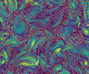
Particle-laden turbulent flows are encountered in many practical applications as in geophysical flows with the dispersion of volcanic ashes, sediment transport or the formation of dunes; in engineering processes with a pulverized coal furnace, pneumatic powder conveying; or in health/medicine with drugs dispersion in the respiratory tract, or the dispersion of a virus by coughing. In all of these examples the physics controlling the particle dispersion is complex because of the multi-physics nature of particle-laden flows. As a non-exhaustive list, one can mention particle-turbulence interaction, turbulence modulation, inter-particle collisions, particle bouncing on smooth or rough walls and inter-particle electrostatic forces. Although it has been neglected over a long time, the effect of the particle charges on the flow dynamics may be very important. As, for example, in electrostatic precipitators, where the granular phase is diluted, particles are charged and an electric field is used to remove the particles from the gas (Parker Reference Parker1997). Also, as denoted by Pruppacher & Klett (Reference Pruppacher and Klett2010), the charges may also have an effect on the coalescence kernel of rain droplets.
This paper focuses on the dispersion of charged solid particles transported by a turbulent gas flow. More precisely, we investigate the self-particle turbulent dispersion (Monin & Yaglom Reference Monin and Yaglom2007) which is characterized by the mean square particle displacement. The particulate flow is very diluted allowing us to neglect turbulence modulation by the particles as well as inter-particle collisions. In such a framework, Li & Ahmadi (Reference Li and Ahmadi1993) investigated the effect of electric charges on the deposition of particles on a flat vertical charged wall. As expected, the authors showed that the electric field leads to an increase of the deposition velocity and the smaller the particle response, the largest is this increase. It is well known that inertial particles suspended in a turbulent fluid flow may concentrate in preferential regions of the turbulence (Fessler, Kulick & Eaton Reference Fessler, Kulick and Eaton1994). This phenomenon, called preferential concentration or clustering, results from the competition between the drag and centrifugal forces. In 2010 Lu et al. (Reference Lu, Nordsiek, Saw and Shaw2010a) analysed experiments to understand how the clustering of solid charged inertial particles is modified by the charges. They show that when particles have the same charge, the Coulomb repulsion force leads to a decrease of the clustering under a given length scale. Theoretical descriptions have also been made to predict the effect of electric charges on the clustering of particles. Alipchenkov, Zaichik & Petrov (Reference Alipchenkov, Zaichik and Petrov2004) for non-settling, and Lu, Nordsiek & Shaw (Reference Lu, Nordsiek and Shaw2010b) for settling particles in a homogeneous isotropic turbulence derived a theoretical expression for the radial distribution function. Particularly, Lu et al. (Reference Lu, Nordsiek and Shaw2010b) validate their model by comparison with experimental measurements obtained for particles having a small Stokes number. The investigation on larger Stokes numbers is generally accomplished by means of numerical simulation. However, as clearly shown by Yao & Capecelatro (Reference Yao and Capecelatro2018) and Boutsikakis et al. (Reference Boutsikakis, Fede, Pedrono and Simonin2020), the way to compute accurately the electrostatic forces in an unbounded domain can be tricky and/or inaccurate. Despite these difficulties, interesting information has been obtained from numerical simulations. As, for example, Lu & Shaw (Reference Lu and Shaw2015) show how the charges modify the collision kernel and especially how they affect the inter-particle relative velocity. In a more complex geometry, namely a turbulent duct, Grosshans et al. (Reference Grosshans, Bissinger, Calero and Papalexandris2021) showed that the charges also affect particle motion at a large scale.
All of these works mainly scrutinized how the electric charges modify the spatial distribution of the particles. However, at first order one can wonder what such an effect would be on particle dispersion. Karnik & Shrimpton (Reference Karnik and Shrimpton2012) slightly addressed this question by showing that the mean variance of particle displacement decreases with increasing particle charges. Boutsikakis et al. (Reference Boutsikakis, Fede, Pedrono and Simonin2020) found similar results and showed that particle agitation intensity decreases for increasing charges. In fact, particle dispersion has two main ingredients: first the particle agitation and second the Lagrangian particle integral time scale. In the present paper, these two contributions are analysed in terms of an electrostatic Stokes number. We show how it is possible to predict the dispersion of like-charged particles by making an analogy between the inter-particle collisions and the Coulomb collisions (i.e. the effect of the electrostatic forces).
The paper is organized as following. The next section gives an overview of the numerical simulations in terms of a direct numerical simulation (DNS) solver and Lagrangian particle tracking. The definitions and the relevance of the characteristic time scales are also discussed. Section 3 is dedicated to the modification of the dispersion coefficient by inter-particle electrostatic forces in terms of dynamic and electrostatic Stokes numbers. Then the analysis is split in two parts: first the modification of particle agitation (§ 4) and then the effect of electrostatic forces on the particle velocity auto-correlation (§5). The conclusions of this work are drawn in the last section.
2. Numerical simulation details
2.1. Direct numerical simulation
Direct numerical simulation of incompressible Navier–Stokes equations has been performed on a cubic domain of length  $L_{b}$ with full three-dimensional periodic boundary conditions. The numerical technique consists of a pseudo-spectral method where aliasing control was ensured by spherical truncation. In order to get a statistically stationary turbulence, the stochastic forcing proposed by Eswaran & Pope (Reference Eswaran and Pope1988) has been used. Such a spectral forcing scheme consists in forcing a given range of wavenumbers by a stochastic force based on a Wiener process. The range of the forced wavenumbers, that control the Eulerian integral length scale of the turbulence,
 $L_f$, has been chosen in order to limit the length of the largest eddies to
 $1/10$ of the domain size. For the variance and the time scale of the Wiener process, we followed the same methodology as Février, Simonin & Squires (Reference Février, Simonin and Squires2005) and Fede & Simonin (Reference Fede and Simonin2006), where they adjust the forcing parameters so that the eddy lifetime turnover time scale
 $T_e=L_f/\sqrt {2q_f^2/3}$ is equal to the Eulerian integral time scale of the turbulence
 $\tau _E=\int _0^{+\infty } R_E(\tau )\,{\rm d}\tau$. The fluid velocity auto-correlation Eulerian function,
 $R_E(\tau )$, is obtained on motionless particles with
 \begin{equation} R_E(\tau) = \frac{\langle \boldsymbol{u}'_{f}(t,\boldsymbol{x}_E)\boldsymbol{u}'_{f}(t+\tau,\boldsymbol{x}_E)\rangle_p}{2q_f^2}, \end{equation}
where  $\boldsymbol {u}'_{f}$ is the fluctuating fluid velocity,
 $q_f^2=1/2\langle \boldsymbol {u}'_{f}\boldsymbol {u}'_{f}\rangle _p$ the fluid kinetic energy (per unit mass) and
 $\langle.\rangle _p$ the average operator over the particles, here the motionless particles. In (2.1),
 $\boldsymbol {x}_E$ is the position of the motionless particles that have been randomly distributed within the domain. Similarly, one can define the Lagrangian fluid velocity auto-correlation function,
 $R_f(\tau )$, as
 \begin{equation} R_f(\tau) = \frac{\langle \boldsymbol{u}'_{f}(t,\boldsymbol{x}_f)\boldsymbol{u}'_{f}(t+\tau,\boldsymbol{x}_f)\rangle_p}{2q_f^2}. \end{equation}
Here,  $\boldsymbol {x}_f$ is the position vector of fluid elements tracked during the numerical simulation. From the Lagrangian fluid velocity auto-correlation function, one obtains the Lagrangian fluid integral time scale by
 $\tau _f^t=\int _0^{+\infty } R_f(\tau )\,{\rm d}\tau$.
Table 1 gathers the relevant parameters and statistics of the turbulent fluid flow (time-averaged statistics have been performed over  ${\sim }45 T_e$). The Kolmogorov length scale is given by
 $\eta _K=(\nu _f/\varepsilon )^{1/4}$, with
 $\varepsilon$ being the dissipation rate measured in DNS, and the Kolmogorov time scale by
 $\tau _K=(\nu _f/\varepsilon )^{1/2}$. Direct numerical simulations have been performed with
 $256^3$ grid points leading to a good resolution of the smallest turbulent scales, as
 $\eta _K\kappa _{max}\approx 3$ (with
 $\kappa _{max}$ being the highest resolved wavenumber).
Properties of the fluid and of the examined HIT.

2.2. Discrete particle simulation
For the particulate phase, we consider a disperse phase composed of  $N_p$ solid, spherical and charged particles. The motion of particles suspended in turbulent flows received much attention (Gatignol Reference Gatignol1983; Maxey & Riley Reference Maxey and Riley1983). In the present case, on one hand, the particle density,
 $\rho _p$, is large compared with that of the fluid, and on the other hand the particle diameter,
 $d_p$, is small compared with the Kolmogorov length scale. Therefore, one can reasonably reduce the forces acting on the particle only to the drag force,
 $\boldsymbol {F}_d$, and the electrostatic force,
 $\boldsymbol {F}_e$. In such a framework, the single particle motion governing equations read as
 $$\begin{gather} \frac{{\rm d}\boldsymbol{x}_p}{{\rm d}t} = \boldsymbol{u}_p, \end{gather}$$
 $$\begin{gather}\frac{{\rm d}\boldsymbol{u}_p}{{\rm d}t} = \frac{\boldsymbol{F}_d}{m_p}+\frac{\boldsymbol{F}_e}{m_p} . \end{gather}$$
Introducing  $\tau _p$, which is the particle response time, the drag force reads as
 \begin{equation} \frac{\boldsymbol{F}_d}{m_p}={-}\frac{f}{\tau_p}(\boldsymbol{u}_p- \boldsymbol{u}_{f@p}), \end{equation}
with  $\tau _p=\rho _pd_p^2/(18\mu _f)$ and
 $f=1+0.15Re_p^{0.687}$ (Schiller & Naumann Reference Schiller and Naumann1935). The particle Reynolds number reads as
 $Re_p=d_p||\boldsymbol {u}_p-\boldsymbol {u}_{f@p} ||/\nu _f$ and
 $\boldsymbol {u}_{f@p}$ is the instantaneous fluid velocity at the particle position undisturbed by the presence of the particle. Since the particle mass fraction is very low, the modulation of the turbulence by the particles (two-way coupling effect) is neglected. Consequently, the fluid velocity seen by the particles is directly computed by a third-order Lagrange polynomial interpolation scheme. For the analysis, one introduces the particle relaxation time scale,
 $\tau _{fp}^{F}$, defined as
 $\tau _{fp}^{F} = \langle\, f/\tau _p\rangle _p^{-1}$.
For two charged particles  $p$ and
 $q$, the electrostatic force that acts on particle
 $p$ due to particle
 $q$ is given by the Coulomb law
 \begin{equation} \boldsymbol{F}_{e,q\rightarrow p} = \lambda\frac{Q_pQ_q}{||\boldsymbol{r}_{pq}||^3}\boldsymbol{r}_{pq} , \end{equation}
where  $\lambda =1/(4{\rm \pi} \epsilon _0)$, with
 $\epsilon _0$ the vacuum permittivity,
 $Q_p$ and
 $Q_q$ the electric charge of the
 $p$ and
 $q$ particle. In (2.6),
 $\boldsymbol {r}_{pq}=\boldsymbol {x}_{p}-\boldsymbol {x}_{q}$ is the distance vector between the two particles pointing to
 $p$. Hence, for a system of
 $N_p$ like-charged particles, each particle interacts with the other
 $N_p-1$ particles, so that the total electrostatic force is
 $\boldsymbol {F}_e=\sum _{q=1,q{\neq} p}^{N_p} \boldsymbol {F}_{e,q\rightarrow p}$. For details of the numerical method, we refer the reader to Boutsikakis et al. (Reference Boutsikakis, Fede, Pedrono and Simonin2020).
2.3. Characteristic time scales and Stokes numbers
In order to compare the effect of electrostatic forces to the entrainment by turbulence, it is important to define a characteristic electrostatic time scale. To characterize the competition between the entrainment by turbulence and the electrostatic force, Alipchenkov et al. (Reference Alipchenkov, Zaichik and Petrov2004) introduced the Coulomb number defined as  $Ct=E_{el}/E_{turb}$. On one hand, as explained by Lu et al. (Reference Lu, Nordsiek, Saw and Shaw2010a),
 $E_{el}=\lambda Q_p^2/(m_p\eta _K)$ is the potential energy due to Coulomb interaction at dissipation scales (namely the Kolmogorov length scale,
 $\eta _K$). On the other hand,
 $E_{turb}=v_K^2$ is the ‘kinetic energy of involvement of particles into small-scale turbulent motion’. Two main drawbacks arise when using such a Coulomb number. First, by definition it concerns only particles interacting with turbulence at the dissipation scale, hence having a small particle response time. Second and more important, such a Coulomb number does not take into account the particle density number. Hence, the analysis based on such a dimensionless number can not be extended to a case with a different number of particles. This last limitation has been overcome by Karnik & Shrimpton (Reference Karnik and Shrimpton2012) by introducing the electric settling velocity
 $v_{el}=\tau _p E_{rms} Q_p/m_p$. Indeed, as
 $E_{rms}$ is the root-mean-square magnitude of the electric field, it is clearly a function of the particle number density. However, the level of
 $E_{rms}$ results from the interactions of particles with turbulence, which can not be known a priori. Karnik & Shrimpton (Reference Karnik and Shrimpton2012) and later Yao & Capecelatro (Reference Yao and Capecelatro2018) compare the electrostatic forces to the entrainment by turbulence with the dimensionless number
 $v_{el}/\sqrt {2q_f^2/3}$. From the particle motion equation, Lu et al. (Reference Lu, Nordsiek, Saw and Shaw2010a) and later Lu & Shaw (Reference Lu and Shaw2015) define the electric settling velocity as the terminal velocity of two particles separated by a distance of the Kolmogorov length scale. The electric settling velocity is then fully written in terms of particle parameters
 $v_{el}= 2 \tau _p Q_p^2/(m_p\eta _K^2)$ and the Coulomb turbulence number becomes
 $Ct=v_{el}/v_K$ (where
 $v_K$ is the Kolmogorov characteristic velocity). Thus, the electric terminal velocity includes two effects, namely the interaction of the particle with the turbulence and the electrostatic forces. Boutsikakis et al. (Reference Boutsikakis, Fede, Pedrono and Simonin2020) proposed another time scale characterizing the electrostatic forces independently of the turbulence itself,
 \begin{equation} \tau_{el} = \frac{1}{Q_p}\sqrt{\frac{3}{2}\frac{m_p}{\lambda n_p}}, \end{equation}
with  $n_p=N_p/L^3$ (where
 $N_p$ is the number of particles) the particle number density. To derive this expression, the authors conducted firstly a dimensional analysis and secondly they performed numerical simulations of like-charged particles in a vacuum. In that case, the particle trajectories are only governed by electrostatic forces. The particle velocity auto-correlation time scale,
 $\tau _p^t$, is hence only dependent to the electrostatic forces and as such, an excellent candidate for being the characteristic time scale of these forces. Such a time scale is defined as the Lagrangian particle integral time scale,
 $\tau _{p}^t=\int _0^{+\infty } R_{p}(\tau )\,{\rm d}\tau$, with the particle velocity auto-correlation function that reads as
 \begin{equation} R_{p}(\tau) = \frac{\langle \boldsymbol{u}'_{p}(t,\boldsymbol{x}_{p}) \boldsymbol{u}'_{p}(t+\tau,\boldsymbol{x}_p)\rangle_p}{2q_{p}^2} , \end{equation}
where  $q_p^2= 1/2\langle \boldsymbol{u}_{p,i}'\boldsymbol{u}_{p,i}'\rangle _p$ is the so-called particle turbulent (or fluctuating) kinetic energy (per unit mass) which is also called the particle agitation in the paper. In figure 1 every marker corresponds to the measurement of
 $\tau _{p}^t$ coming from a different simulation with a different set of particle properties. All simulations concern like-charged particles of diameter
 $d_p=5\times 10^{-3}\ {\rm m}$ in a tri-periodic computational domain of size
 $L_b$ (see table 1). In order to perform the dimensional analysis, the following particle properties have been considered:
 $\rho _p = \{1.5, \boldsymbol {2.75}, 5, 10 ,20\}\times 10^3, Q_p = \{2, 3, 4, \boldsymbol {5}, 6\}\times Q_0, N_p = \{1, 2.5, 5, \boldsymbol {10}, 25, 50, 100, 150\}\times 10^3$, where the values in bold correspond to the reference simulation and each other simulation entails only one parameter change. This figure shows the excellent agreement of the measured electrostatic time scale with the proposed characteristic time scale of electrostatic forces given by (2.7). One emphasizes that (2.7) differs slightly from the original expression proposed by Boutsikakis et al. (Reference Boutsikakis, Fede, Pedrono and Simonin2020). The difference is only the coefficient
 $\sqrt {3/2}$ that we have introduced from correlation analysis on dry granular charged flows.
Comparison of particle velocity auto-correlation time scale measured in homogeneous isotropic dry granular flow of charged particles with the characteristic time scale of electrostatic forces proposed by Boutsikakis et al. (Reference Boutsikakis, Fede, Pedrono and Simonin2020) and given by (2.7).

To better understand the competition between inter-particle electrostatic forces and particle-turbulence interaction, we defined several dimensionless numbers (i.e. several Stokes numbers) based on previous time scales. Firstly, for the dynamics of the particles, one can introduce the standard (dynamic) Stokes number defined as the ratio between the particle relaxation time scale  $\tau _{fp}^F$ to the Lagrangian fluid integral time scale seen by inertial particles,
 $\tau _{f@p}^t$ (Deutsch & Simonin Reference Deutsch and Simonin1991). This last time scale is defined by
 $\tau _{f@p}^t=\int _0^{+\infty } R_{f@p}(\tau )\,{\rm d}\tau$ with the auto-correlation function of the fluid velocity seen by the particles that reads as
 \begin{equation} R_{f@p}(\tau) = \frac{\langle \boldsymbol{u}'_{f@p}(t,\boldsymbol{x}_{p})\boldsymbol{u}'_{f@p}(t+\tau,\boldsymbol{x}_p)\rangle_p}{2q_{f@p}^2} . \end{equation}
In (2.9) the auto-correlation function is normalized by the fluid kinetic energy (per unit mass) seen by the particles which is given by  $q_{f@p}^2=1/2\langle \boldsymbol {u}_{f@p}'\boldsymbol {u}_{f@p}'\rangle _p$. To compare the electrostatic forces to the particle-turbulence interaction, we introduce the electrostatic Stokes number as
 $\tau _{fp}^F / \tau _{el}$. The asymptotic behaviour of the electrostatic Stokes number is obvious. Indeed, for
 $\tau _{fp}^F / \tau _{el}\rightarrow 0$, the inter-particle electrostatic forces are negligible, and the particle dispersion is controlled by the turbulence. In contrast, for
 $\tau _{fp}^F / \tau _{el}\rightarrow +\infty$, particle dynamics is controlled by electrostatic forces.
In the present numerical simulations, the particle diameter has been conserved constant,  $d_p/\eta _K=0.2$, and the particle density varies in order to obtain different values of dynamic Stokes number. With
 $\rho _p/\rho _f\in [200,20\,000]$, it leads to a range of dynamic Stokes number from
 $0.073$ to
 $6.39$. Since particle diameter is smaller than the Kolmogorov scale, particles are numerically treated under the point-particle approximation. As such, the particle charge
 $Q_p$ is considered to be concentrated at one point (particle's centre of mass) defined as
 $Q_p={\rm \pi} d_p^2\rho _Q$, where
 $\rho _Q$ is the particle surface charge density. It should be noted here, that according to Hamamoto, Nakajima & Sato (Reference Hamamoto, Nakajima and Sato1992) there is a saturation limit of surface charge density for small spheres, which can be translated (via
 $d_p$) to a corresponding limit for point-particle charges.
For the configuration presented in this work, this value can be estimated to be approximately 4 nC. The various particle charges, that have been considered, are all given in terms of a reference charge  $Q_0=1$ nC (Boutsikakis et al. Reference Boutsikakis, Fede, Pedrono and Simonin2020) which is of the same order of magnitude as the aforementioned limit. To explore the effect of electrostatic forces through the electrostatic Stokes number, particle charge varies from
 $0.1Q_0$ to
 $10Q_0$ which leads to an electrostatic Stokes variation in the range of
 $3\times 10^{-3}$ to
 $2.8$. Figure 2 shows all dynamic and electrostatic Stokes numbers investigated in the present paper.
Dynamic ( $\tau _{fp}^F/\tau _{f@p}^t$) and electrostatic Stokes (
 $\tau _{fp}^F/\tau _{el}$) numbers of the numerical simulations used in the study. Each point corresponds to a case differing by the dynamic Stokes number or by the electrostatic Stokes number.

3. Effect of electrostatic forces on the dispersion of charged particles
In this section we first examine how the particle dispersion coefficient is affected by electrostatic forces. The dispersion of solid particles transported by a turbulent flow has been extensively investigated, for example, by Tchen (Reference Tchen1947), Hinze (Reference Hinze1972), Gouesbet, Berlemont & Picart (Reference Gouesbet, Berlemont and Picart1982, Reference Gouesbet, Berlemont and Picart1984), Deutsch & Simonin (Reference Deutsch and Simonin1991), Simonin, Deutsch & Minier (Reference Simonin, Deutsch and Minier1993) and Pascal & Oesterlé (Reference Pascal and Oesterlé2000). Mathematically, the dispersion coefficient,  $D_p^t$, is related to the variance of particle displacement. Hence, it is defined as
 \begin{equation} D_p^t = \lim_{\tau\rightarrow+\infty} \frac{1}{6}\frac{{\rm d}}{{\rm d}\tau}\langle (\boldsymbol{x}_{p}(t+\tau)-\boldsymbol{x}_{p}(t))^2\rangle_p . \end{equation}
Figure 3 shows the time evolution of the particle displacement variance measured in DNS. After a transitory phase, the variance of displacement has a linear evolution. To compute the dispersion coefficient over long times, a linear regression is performed for the last  $45\,\%$ of the temporal signal (after the vertical line on figure 3) and the slope corresponds to the dispersion coefficient.
Time-evolution of the mean square displacement of particles for  $\tau _{fp}^F/\tau _{f@p}^t=6.39$ (a) and
 $\tau _{fp}^F/\tau _{f@p}^t=0.073$ (b). Symbols represent the data from DNS, while solid lines the linear regression performed on the data at long times, namely after the vertical lines. Plot (a) shows electrostatic Stokes numbers
 $\tau _{fp}^F/\tau _{el} = 1.63$ (
 $Q_p=5.0Q_0$) and
 $\tau _{fp}^F/\tau _{el} = 3.27$ (
 $Q_p=10.0Q_0$). Plot (b) shows electrostatic Stokes numbers
 $\tau _{fp}^F/\tau _{el} = 0.18$ (
 $Q_p=5.0Q_0$) and
 $\tau _{fp}^F/\tau _{el} = 0.35$ (
 $Q_p=10.0Q_0$).

As a classic result, the time for reaching the established dispersion depends on the particle relaxation time scale. The smaller the relaxation time scale, the shorter the transient period. Concerning the effect of the electric charge, one observes that particle dispersion decreases with increasing the charge.
Figure 4 shows the particle dispersion coefficient normalized by the value in the charge-free case with respect to both the dynamic and electrostatic Stokes numbers. We first observe that for a small electrostatic Stokes number (i.e.  $\tau _{fp}^F/\tau _{el}<0.1$), there is no effect of the charges on the particle dispersion coefficient. In contrast, for
 $\tau _{fp}^F/\tau _{el}>0.1$, the dispersion coefficient decreases with increasing the electrostatic Stokes number. That trend is observed for all dynamic Stokes numbers, and it can be noticed that for the smallest Stokes number
 $\tau _{fp}^F/\tau _{f@p}^t=0.073$, the modification by inter-particle electrostatic forces is smaller than for the particles with the highest Stokes number
 $\tau _{fp}^F/\tau _{f@p}^t=6.39$. For the latter, the decrease of particle dispersion is up to
 $60\,\%$.
Effect of the charge on the particle dispersion coefficient with respect to the dynamic Stokes number and the electrostatic Stokes number.

In homogeneous isotropic turbulent flows the dispersion coefficient may also by computed with the expression (Hinze Reference Hinze1972)
 \begin{equation} D_p^t = \tfrac{2}{3}q_p^2 \tau_p^t, \end{equation}
where we remind that  $q_p^2= 1/2\langle \boldsymbol{u}_{p,i}'\boldsymbol{u}_{p,i}'\rangle _p$ is the particle kinetic energy (per unit mass) and
 $\tau _{p}^t=\int _0^{+\infty } R_{p}(\tau )\,{\rm d}\tau$ is the Lagrangian particle integral time scale with the particle velocity auto-correlation function,
 $R_p$, defined by (2.8).
Figure 5 shows that for all charges and all particle inertia, the deviation between the measured particle dispersion coefficient and the Tchen–Hinze theoretical model (3.2) is less than 5 %. It means that even if the particle dispersion coefficient is modified by the inter-particle electrostatic forces, the relation between the dispersion coefficient to the particle agitation and the Lagrangian particle integral time scale remains unchanged. From this, in the following sections we scrutinize how the particle agitation and the particle velocity auto-correlation time scale are both modified by the electrostatic forces.
Measured particle dispersion coefficient normalized by the model standard expression (3.2) with respect to dynamic (a) and electrostatic Stokes numbers (b).

4. Modification of particle kinetic energy and fluid–particle velocity covariance by electrostatic forces
The modulation of particle kinetic energy by electrostatic forces is shown by Figure 6. As expected, for small values of the electrostatic Stokes number, the particle agitation is found unchanged by the electrostatic forces. For  $\tau _{fp}^F/\tau _{el}>5\times 10^{-2}$, non-monotonic modifications of the particle agitation are observed. As, for example, considering the case of
 $\tau _{fp}^F/\tau _{f@p}^t=0.13$ for an increasing electrostatic Stokes number, the particle agitation increases first and then decreases for large values of the electrostatic Stokes number. The same behaviour is also observed for larger values of the dynamic Stokes number.
Effect of the electrostatic charges on the particle kinetic energy with respect to the dynamic Stokes number and to the electrostatic Stokes number.

Such evolution could be surprising because the inter-particle electrostatic forces are conservative and should not modify the particle kinetic energy. However, as shown by Boutsikakis et al. (Reference Boutsikakis, Fede, Pedrono and Simonin2020), the modulation of the particle kinetic energy by the electrostatic forces is, in fact, an indirect effect due to the modification of the fluid–particle covariance  $q_{fp}=\langle \boldsymbol{u}_{p,i}'\boldsymbol{u}_{f@p,i}'\rangle _p$ by electrostatic forces. Indeed, following the Tchen–Hinze theory, the particle kinetic energy is related to the fluid–particle velocity covariance by Tchen (Reference Tchen1947) (see also Hinze Reference Hinze1972 or Gouesbet et al. Reference Gouesbet, Berlemont and Picart1984) as
 \begin{equation} 2q_p^2 = q_{fp} . \end{equation}
Figure 7 shows (4.1) with respect to the electrostatic Stokes number. One can observe that, for the wide range of investigated electrostatic Stokes numbers, the relation (4.1) is always satisfied. In the present case, figure 6 shows a maximum modification of the particle kinetic energy on the order of  $20\,\%$ that can not explain, just by itself, the modification of the particle dispersion coefficient (see figure 4).
Effect of the electrostatic charges on the Tchen–Hinze equilibrium defined by (4.1).

In the framework of the joint probability density function (PDF) approach (see Zaichik, Simonin & Alipchenkov Reference Zaichik, Simonin and Alipchenkov2003, Reference Zaichik, Simonin and Alipchenkov2006; Reeks, Simonin & Fede Reference Reeks, Simonin and Fede2016 for details), it is possible to derive the following transport equation for the fluid–particle velocity covariance (Deutsch & Simonin Reference Deutsch and Simonin1991; Simonin Reference Simonin1996):
 \begin{equation} \frac{{\rm d}q_{fp}}{{\rm d}t} = \left\langle\frac{\boldsymbol{F}_d}{m_p} \boldsymbol{u}_{f@p}'\right\rangle_p +\langle \boldsymbol{a}_{f@p}' \boldsymbol{u}_{p}'\rangle_p +\left\langle\frac{\boldsymbol{F}_e}{m_p}\boldsymbol{u}_{f@p}' \right\rangle_p. \end{equation}
Here  $\boldsymbol {a}_{f@p}={\rm d}\boldsymbol {u}_{f@p}/{{\rm d}t}$ is the acceleration of the fluid seen by the particles. In (4.2) the first term on the right-hand-side is the effect of the entrainment by fluid turbulence due to drag force on the fluid–particle covariance. With (2.5) this term reads as
 \begin{equation} \left\langle\frac{\boldsymbol{F}_d}{m_p}\boldsymbol{u}_{f@p}'\right\rangle_p ={-} \frac{q_{fp}-2q_{f@p}^2}{\tau_{fp}^F}, \end{equation}
where two contributions appear: first, a dissipative term by the viscous friction of the particles with the fluid and, second, the transfer of kinetic energy from the turbulence towards the particles. The second term in (4.2) represents the correlation between the acceleration of the fluid seen by the particles and the particle fluctuating velocity. Figure 8 shows the evolution of this term with respect to the dynamic and electrostatic Stokes numbers. From the left panel it can be observed that, even without electric charge, this term depends on the dynamic Stokes number. The two asymptotic trends were expected because, on one hand, when particle inertia is large, the particle velocity is uncorrelated with the fluid velocity and acceleration, hence,  $\langle \boldsymbol {a}_{f@p}' \boldsymbol {u}_{p}'\rangle _p \rightarrow 0$. On the other hand, when the particle relaxation time scale is very small hence
 $\langle \boldsymbol {a}_{f@p}' \boldsymbol {u}_{p}'\rangle _p \rightarrow \langle \boldsymbol {a}_{f}' \boldsymbol {u}_{f}'\rangle _f$ but in stationary homogeneous isotropic turbulent flow
 $\langle \boldsymbol {a}_{f}'\boldsymbol {u}_{f}'\rangle _f \rightarrow 0$. When the electrostatic Stokes number increases, figure 8 shows that
 $\langle \boldsymbol {a}_{f@p}' \boldsymbol {u}_{p}'\rangle _p$ is decreasing. As a direct conclusion, the electrostatic forces lead to a decrease of the correlation between the particle velocity and the local fluid acceleration. Furthermore, such a destruction of the fluid–particle velocity covariance is even larger for larger dynamic Stokes numbers.
Fluid–particle interaction term with respect to the dynamic (a) and the electric (b) Stokes numbers.

Finally, the last term on the right-hand side of (4.2) is the effect of the electrostatic forces on the fluid–particle covariance. Figure 9 shows this term measured in the DNS with respect to the electrostatic Stokes number. Such a term is found negative, meaning that the electrostatic force destructs the fluid–particle covariance. As expected, this term increases when the electrostatic Stokes number increases. Figure 6 shows a non-monotonic evolution of the particle kinetic energy as a function of the electrostatic Stokes number which can be explained as follows. Indeed, considering the relevant case of  $\tau _{fp}^F/\tau _{f@p}^t=0.13$, when
 $\tau _{fp}^F/\tau _{el}$ is larger than
 $5\times 10^{-2}$, we observe an increase of
 $q_p^2$. This is explained by the fact that the electrostatic forces decrease the intensity of
 $\langle \boldsymbol {a}_{f@p}' \boldsymbol {u}_{p}'\rangle _p$, which is negative (see figure 8a). As a result, the fluid–particle velocity covariance increases and consequently does the particle kinetic energy. At that time, the direct destruction of the fluid–particle covariance by electrostatic forces also acts but its effect is weak. However, for approximately
 $\tau _{fp}^F/\tau _{el}>2\times 10^{-1}$, this direct destruction term dominates, leading to the decrease of the particle kinetic energy.


To model the effect of the electrostatic forces, it is possible to make an analogy with elastic inter-particle collisions. Fundamentally, the main difference is the collision distance, which is, for the latter, the particle diameter (i.e. two colliding particle have to be in contact). For the electrostatic force, collisions occur at a given effective distance larger than the particle diameter (note that in the literature dedicated to the plasma, the terminology ‘Coulomb collisions’ is used to denote electrostatic interactions). This analogy leads to two consequences. First, the inter-particle collision time scale  $\tau _{col}$, which is the time for one particle to have a collision with any other particle, may be substituted by the characteristic time scale of electrostatic forces
 $\tau _{el}$. Second, the electrostatic effect in the PDF approach can be treated as a collision with a frequency
 $1/\tau _{el}$ and occurring at the effective distance
 $d_{el}$. This last parameter can be estimated from works done in plasma where they estimate the Coulomb collision cross-section by
 \begin{equation} d_{el}=\frac{1}{2{\rm \pi} \epsilon_0}\frac{Q_p^2}{m_p\langle ||\boldsymbol{w}_{r}||\rangle_p^2}, \end{equation}
where  $\boldsymbol {w}_{r}$ is the inter-particle relative velocity that is given by
 $\langle ||\boldsymbol {w}_{r}||\rangle _p=\sqrt {32q_p^2/(3{\rm \pi} )}$. The analogy between inter-particle collisions and Coulomb collisions allows us to explain why the fluid–particle covariance decreases with the electrostatic forces, and also to model this said destruction. First, in case of elastic inter-particle collisions, Laviéville et al. (Reference Laviéville, Simonin, Berlemont and Chang1997) and later Fede, Simonin & Villedieu (Reference Fede, Simonin and Villedieu2015) explained that if particles are smaller than the smallest turbulent scale (i.e. the Kolmogorov length scale), two colliding particles see nearly the same velocity. As a matter of fact, the fluid–particle covariance of the two colliding particles is conserved because of the conservation of momentum (reminder that only elastic collisions are considered).
To explain a pathological non-physical destruction of the fluid–particle covariance, observed in the Lagrangian stochastic approach, Laviéville et al. (Reference Laviéville, Simonin, Berlemont and Chang1997) (see also Sommerfeld Reference Sommerfeld2001; Fede et al. Reference Fede, Simonin and Villedieu2015; Fede & Simonin Reference Fede and Simonin2018) derived analytically the fluid–particle destruction term at a given distance. Replacing the collision time scale with the electric one, it is written as
 \begin{equation} \left\langle\frac{\boldsymbol{F}_e}{m_p} \boldsymbol{u}_{f@p}\right\rangle_p ={-}\frac{2}{3}[1-f(d_{el})]\frac{q_{fp}}{\tau_{el}}, \end{equation}
where  $f(r)$ is the fluid velocity spatial auto-correlation function, with the asymptotic behaviours
 $f(r=0)=1$ (more precisely it is for
 $r<\eta _K$) and for large distances
 $\lim _{r\rightarrow +\infty }f(r)=0$. In first approximation, such a function can be approximated using an exponential function
 \begin{equation} f(r)=\exp\left[-\frac{r}{L_f}\right], \end{equation}
but, for short distances, a two-exponential model can be used,
 \begin{equation} f(r)=\frac{\exp\left[-\dfrac{\chi^2r}{L}\right]-\chi^2\exp\left[-\dfrac{r}{L}\right]}{1-\chi^2}, \end{equation}
where  $\chi$ and
 $L$ are the solutions of
 $L=L_f(1+{1}/{\chi ^2})^{-1}$ and
 $\chi ={L}/{\lambda _g}$. A similar two-scale model has also been proposed by Sawford (Reference Sawford1991) for the fluid velocity Lagrangian auto-correlation function. The choice of the model may lead to differences in the predictions of the fluid–particle velocity covariance destruction by (4.5). Figure 10 shows the relative position of the Coulomb collision diameter
 $d_{el}$ to the Eulerian integral length scale,
 $L_f$, with respect to both models and also with regards to the dynamic Stokes number.


Figure 9 shows the comparison between  $\langle \boldsymbol {F}_e \boldsymbol {u}_{f@p}\rangle _p /m_p$ measured in DNS and the predictions given by (4.5). The dashed lines correspond to the original model proposed by Laviéville et al. (Reference Laviéville, Simonin, Berlemont and Chang1997) corresponding to
 $d_{el}\gg L_f$, hence,
 $f(d_{el})=0$. The solid lines are the prediction with (4.7) and (4.4). Two main conclusions can be drawn from figure 9. First, the electrostatic term is negative, hence, it is really a destruction term of the fluid–particle velocity covariance. Second, the model predictions are in agreement with the DNS data.
5. Effect of electrostatic forces on the particle velocity auto-correlation
To investigate the effect of the electrostatic forces on the Lagrangian particle integral time scale, one can start first by the particle velocity auto-correlation function. These correlation functions are given by figure 11. As expected, when the electric charge is increasing, the auto-correlation function decreases because the electrostatic forces decorrelate the particle velocities. Such an effect is found to be more important for a large dynamic Stokes number (left panel). As a direct consequence, the integral of the auto-correlation functions decrease for increasing particle charge. The decrease of the Lagrangian particle integral time scale with the dynamic Stokes number is shown by figure 12. Such a figure also shows a standard result, which is the increase of the Lagrangian particle integral time scale for increasing Stokes number (i.e. the larger the particle inertia, the longer the particle velocity is correlated with itself).
Effect of the electrostatic charges on the particle velocity auto-correlation function for  $\tau _{fp}^F/\tau _{f@p}^t=6.39$ (a),
 $\tau _{fp}^F/\tau _{f@p}^t=0.97$ (b) and
 $\tau _{fp}^F/\tau _{f@p}^t=0.073$ (c).

Lagrangian particle integral time scale normalized by the Lagrangian fluid integral time scale with respect to the dynamic Stokes number.

For the modelling of particle dispersion, a model is needed for the integral of the particle velocity auto-correlation function, namely the Lagrangian particle integral time scale  $\tau _p^t$, but also for the shape of the auto-correlation function. To show how the electrostatic forces modify the shape of the auto-correlation function, figure 13 shows these functions with respect to the time normalized by the Lagrangian particle integral time scale. For a small dynamic Stokes number, the electrostatic forces have no effect on the shape of
 $R_p(\tau )$, and for a larger Stokes number, we observe that the particle velocity auto-correlation function tends to an exponential function. These differences occur essentially for a short time
 $\tau \rightarrow 0$.
Effect of the electrostatic charges on the shape of the particle velocity Lagrangian auto-correlation function for  $\tau _{fp}^F/\tau _{f@p}^t=6.39$ (a),
 $\tau _{fp}^F/\tau _{f@p}^t=0.97$ (b) and
 $\tau _{fp}^F/\tau _{f@p}^t=0.073$ (c).

Laviéville, Deutsch & Simonin (Reference Laviéville, Deutsch and Simonin1995) analysed the effect of inter-particle collisions on the dispersion of particles transported by homogeneous isotropic turbulence. The authors derived theoretically the expressions of the particle velocity auto-correlation function, Lagrangian particle integral time scale and particle dispersion coefficient taking into account the effect of the collisions. Making an analogy between particle collisions and Coulomb collisions, the particle velocity auto-correlation function proposed by Laviéville et al. (Reference Laviéville, Deutsch and Simonin1995) can be rewritten as
 \begin{equation} R_p(\tau) = \exp\left(-\frac{\tau}{\tau_b}\right)+\frac{\tau_{f@p}^t \tau_b}{\tau_{fp}^F} \frac{\exp\left(-\dfrac{\tau}{\tau_b}\right)-\exp\left(-\dfrac{\tau} {\tau_{f@p}^t}\right)}{\tau_b-\tau_{f@p}^t} , \end{equation}
where  $\tau _b=\tau _{fp}^F[1+\frac {2}{3}({\tau _{fp}^F}/{\tau _{el}})]^{-1}$. This model is based on two time scales, which is strictly equivalent to saying it is a two-exponential model. As shown by Deutsch & Simonin (Reference Deutsch and Simonin1991), in case of no collisions (
 $\tau _{fp}^F/\tau _{el}\rightarrow 0$), the question of the one- or two-exponential model depends on the dynamic Stokes number. For a small Stokes number and/or fluid elements, the slope at the origin depends on the Reynolds number. A one-exponential model is more suitable for a high Reynolds number, and a two-exponential one is more adapted to a low Reynolds number (Sawford Reference Sawford1991). For moderate and large Stokes numbers, particle inertia leads the particle velocity to be correlated over a short time giving a non-zero slope of the auto-correlation function. Such an effect can be taken into account by the original model proposed by Laviéville et al. (Reference Laviéville, Deutsch and Simonin1995). If the characteristic time scale of these mechanisms is smaller than the particle relaxation time scale, they asymptotically tend towards the single-exponential function.
The Lagrangian particle integral time scale with respect to the electrostatic Stokes number is shown by figure 14. As expected, the decorrelating effect of the electrostatic forces leads to the decreasing of the Lagrangian particle integral time scale. The magnitude of such a decrease explains why the particle dispersion coefficient decreases so strongly when the electrostatic Stokes number increases (see figure 4). From the auto-correlation function (5.1), Laviéville et al. (Reference Laviéville, Deutsch and Simonin1995) derived theoretically the evolution of the Lagrangian particle integral time scale as a function of the inter-particle collision time scale. Replacing such a time scale by the characteristic one of the electrostatic forces leads to the following expression:
 \begin{equation} \frac{\tau_p^t}{\tau_{f@p}^t}=\left[1+\frac{\tau_{fp}^F}{\tau_{f@p}^t} \right]\times \left[1+\frac{2}{3}\frac{\tau_{fp}^F}{\tau_{el}}\right]^{{-}1}. \end{equation}
Figure 14 compares the prediction of (5.2) with our DNS data. The left panel is an a priori test, in the sense that the model predictions are computed with our DNS data. It has to be contrasted with the right panel where  $\tau _{f@p}^t$ and
 $\tau _{fp}^F$ of the charge-free cases have been used for computing the model predictions. Figure 14 shows a good agreement between the DNS and the model predictions.
Lagrangian particle integral time scale with respect to the electrostatic Stokes number. Symbols represent the statistics from DNS, while lines the prediction of (5.2). (a) The model is computed with the DNS data (a priori test). (b) The model is computed with the data of the charge-free case.

The last step of this study consists of the prediction of the particle dispersion coefficient modulation by electrostatic forces. As previously stated, we propose drawing an analogy between the inter-particle and Coulomb collisions. Following the model proposed by Laviéville et al. (Reference Laviéville, Deutsch and Simonin1995), the particle dispersion coefficient can be predicted by
 \begin{equation} D_p^t = \frac{2}{3}q_p^2\tau_{fp}^F \left[1+\frac{\tau_{f@p}^t}{\tau_{fp}^F}\right]\times \left[1+\frac{2}{3}\frac{\tau_{fp}^F}{\tau_{el}}\right]^{{-}1} . \end{equation}
Figure 15 shows the comparison between DNS data and predictions given by (5.3). As for figure 14, the left panel shows model predictions that have been computed with the DNS data and the right panel with the data from the charge-free cases. A very good agreement is observed between the model and the DNS data.
Particle dispersion coefficient with respect to the electrostatic Stokes number. Symbols represent the statistics from DNS, while lines the prediction of (5.3). (a) The model is computed using the data from DNS (a priori test). (b) The model is computed with the data of the charge-free case.

6. Conclusions
The paper analyses the effects of electrostatic forces on the dispersion of like-charged inertial particles transported by homogeneous isotropic turbulent flows. Direct numerical simulation coupled with Lagrangian tracking of charged particles have been performed, where the particle motion is controlled only by the drag and electrostatic forces. According to the very low solid volume fraction considered, both two-way coupling and inter-particle collisions are neglected.
The numerical simulations show that the particle dispersion coefficient decreases when the electrostatic Stokes number is increasing. Since the dispersion of particles by turbulent flow is related to the particle agitation intensity and also to the Lagrangian integral time scale of the particle velocities, these two quantities have been analysed with respect to the dynamic and electrostatic Stokes numbers.
As already shown by Boutsikakis et al. (Reference Boutsikakis, Fede, Pedrono and Simonin2020), particle agitation decreases with increasing electrostatic Stokes number. However, the local equilibrium between the particle agitation and the fluid–particle covariance is still satisfied, namely  $2q_p^2=q_{fp}$. Hence, the destruction of particle agitation by electrostatic forces is an indirect effect, because it comes from the destruction of the fluid–particle covariance
 $q_{fp}$. When analysing the transport equation of the latter, we show that the electrostatic forces have two effects. First, they decrease the correlation between the fluid acceleration and the particle velocity (indirect effect). Second, the electrostatic forces act as a destruction term of the fluid–particle covariance (direct effect). The non-monotonic evolution of the particle kinetic energy results from the competition of these two effects. Treating electrostatic interactions as Coulomb collisions, the model proposed by Laviéville et al. (Reference Laviéville, Deutsch and Simonin1995), for predicting the fluid–particle covariance destruction by inter-particle collisions, has been compared with the DNS results. We show that if the collision time scale is replaced by the electrostatic time scale, it is possible to predict the destruction of the fluid–particle covariance. As expected, the Lagrangian particle integral time scale is found decreasing when increasing the electrostatic Stokes number because of the decorrelating nature of the (repulsive) electrostatic forces. Again, we show that the predictions of the model proposed by Laviéville et al. (Reference Laviéville, Deutsch and Simonin1995) are in agreement with the DNS.
From a modelling point of view, we show that the models proposed for inter-particle collisions can be used for predicting the like-charged particle dispersion in turbulent flows. However, these models assume that the spatial distribution of the particles is uniform, i.e. no preferential concentration. Moreover, it has been shown by Lu et al. (Reference Lu, Nordsiek, Saw and Shaw2010a) that electrostatic forces may modify the spatial particle distribution through the modification of the radial distribution function.
Acknowledgements
The numerical simulations have been performed on the supercomputer hosted by the meso-scale supercomputer center CALMIP (project P0111) as well as by the French national supercomputer center CINES (Allocation A0102B06012, A0082B06012, A0062B06012).
Declaration of interests
The authors report no conflict of interest.


 Open access

