Our congressional forecasting model provides predictions of individual House and Senate races as well as aggregate party seat shares in each chamber. It does so by marrying an underlying structural or “fundamentals”-based model with available polling data—an approach similar to Linzer (Reference Linzer2013).

The structural portion of the model is based on contested House and Senate elections from 1980 to 2012, excluding those when an independent or third-party candidate won a significant share of the vote. ^{Footnote 1} The dependent variable is the Democratic candidate’s share of the major-party vote. The independent variables are drawn from the extensive literature that has identified significant national and state or district correlates of congressional election outcomes (e.g., Jacobson Reference Jacobson2012). These include:

• • The nonannualized change in real gross domestic product (GDP) in the first two quarters of the election year.

• • The president’s average approval rating in June of the election year.

• • Whether it is a midterm or presidential election year.

• • Whether the seat is being contested by a Republican incumbent, a Democratic incumbent, or no incumbent (i.e., it is an open seat).

• • The Democratic Party’s share of the two-party presidential vote in each political unit (states or districts) in the concurrent or most recent election (mean-deviated by election year).

• • Relative candidate quality, which is the difference between the Democrat’s level of previous elective office experience and the Republican’s. For House races, experience is coded as a dichotomy, distinguishing candidates who have held at least some elective office from candidates who have held no such office. For Senate races, each candidate is coded on a six-point scale: no elective office; a local office or state legislator; a statewide office other than governor (including former US senators); US House or large city mayor; governor; or incumbent US senator.

• • The Democratic candidate’s share of spending by the two major-party candidates.

For Senate elections, the model also includes:

• • The previous Democratic vote share for the seat. The effect of this variable is allowed to vary by whether the incumbent senator is running for reelection. (Including lagged vote share in the model of House elections requires excluding election years that follow redistricting.)

• • Whether an appointed senator is running for his or her first election, and that senator’s party.

All variables are coded so that higher values capture better circumstances for Democratic candidates. For the three national-level variables, we multiply each by a variable for the president’s party (–1=Republican; +1=Democrat) and also include that indicator in the model.

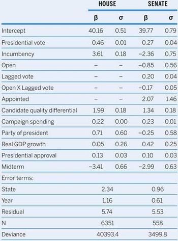
We account for uncertainty in our forecasts by assigning probabilities to all our predictions based on the error parameters in our models (Lauderdale and Linzer Reference Lauderdale and Linzer2014). Likewise, because the structural model cannot account for all the factors that make each state and election year unique, we estimate a multilevel model with random intercepts for states and years so we can propagate that uncertainty more precisely into our predictions. ^{Footnote 2} The results of the structural model for both House and Senate elections are shown in table 1.

Table 1

Parameter Estimates of Contested House and Senate Election Outcomes, 1980−2012

Across the two types of elections notable similarity exists in the apparent effects of presidential approval and the midterm penalty. The estimated effects of campaign spending are also almost identical across the models. The estimate for presidential vote is larger for House elections, but that may be due to the inclusion of previous vote in the Senate models because both variables tap the local partisan balance. Also note that several candidate-related variables—incumbency, appointed, and quality differential—are not comparable across the election types because of the differences in model specification and measurement noted previously.

These parameter estimates may be used to make predictions for the 435 House and 36 Senate elections this year. We do this by substituting the 2014 values for each of the elections and computing the predicted vote shares. (Because final spending amounts will not be available until well after November, we use the most recent figures for fundraising during the 2013–2014 cycle.) Our estimates take into account uncertainty about the model parameters (the standard errors of the coefficients) along with the overall uncertainty in the model. In this process, the random error terms for years and states can be thought of as “offsets” that identify how each year or state differed from all others for unmeasured reasons. The multilevel model constrains these offsets to collectively form a normal distribution with mean zero and a variance estimated from the data. In addition to capturing the unmeasured variance, the offsets also contain estimation uncertainty—that is, uncertainty as to the precise value of each offset—which we also include in the predictions.

To produce our predictions, we simulate 1,000 outcomes for each election by drawing from the distributions estimated from the structural model discussed previously. ^{Footnote 3} When doing so, we treat the year and state error terms somewhat differently. Because we do not know what kind of election year we will have, we draw from a normal distribution with the same mean (i.e., zero) and variance as the year error term and add these values to our predictions. By contrast, we know that the elections will be conducted in the same set of states as before, so we can simply add those state offsets to our predictions in something more closely approximating a “fixed effects” approach, while also accounting for the estimation uncertainty in the offsets. With these simulated elections, we make predictions about individual races and overall partisan seat distributions by aggregating our individual predictions and the uncertainty that comes with them.

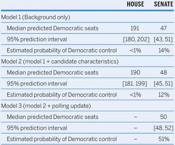
Following the suggestion of Sides (Reference Sides2014) that forecasters estimate “heuristic” models that focus on different sets of key factors, we present the forecasts of different versions of the structural model in table 2. For each model, we present the predicted number of Democratic seats, the associated 95% prediction interval, and the estimated probability that the chamber will have a Democratic majority. ^{Footnote 4} Models 1 and 2 in table 2 present two versions of the model. The first takes into account background characteristics of the election that are outside of candidates’ control. The second builds in characteristics of the candidates.

Table 2

Predicted Party Division of Seats for the House and Senate

Note: Model 1 includes all the structural variables except the candidate quality differential and campaign spending. Model 2 includes those variables as well, and model 3 updates the model 2 forecast in a Bayesian fashion using the available polling data. See text for details. Note that, because Democratic vice president Joe Biden can serve as a tie-breaking vote in the Senate, the Democrats would retain control of that chamber with 50 seats.

At some points in the past, these two models produced different results, at least for the Senate. But as of now their predictions are very similar. The point prediction for Democratic seats hardly changes; the main difference is in the size of the confidence interval. Adding information about the candidates decreases the confidence interval, but the absence of movement in the point prediction also suggests that candidate quality and spending are roughly balanced between the two parties in the aggregate. ^{Footnote 5} On the House side, both models give the Republicans overwhelming odds of retaining control. For the Senate, both models are also favorable to the Republicans, giving the Democrats only about a one-in-five chance of retaining control.

The most valuable additional information that can be systematically incorporated into our predictions is polling data from individual elections, which are only available for the Senate contests. To do this we first compute the Democratic share of major-party vote intentions in each poll. Then, race by race, we estimate the current Democratic poll share and its standard error based on a local regression smoother (loess) with a bandwidth of 1.5. Standard errors for the predictions become progressively larger as a function of the variance in the polls themselves and the number of days since the last poll. In addition, to ensure that we properly account for uncertainty in these polls, we also bootstrapped 1,000 loess models based on the means and sample sizes of each poll. This sampling variance was then added to the loess model variance to obtain a total variance for the polling estimate.

The last step is to combine the estimated poll standing and predicted vote shares. Following Jackman (Reference Jackman2004), we treat the structural prediction as a Bayesian prior, which is then updated with information from the polls. The weight attached to each component—the structural forecast and the polling estimate—is a function of their relative variances as well as a scaling parameter that inflates or deflates the variance of the structural forecast based on our confidence in this prior. ^{Footnote 6} Simply put, estimates with less variance receive greater weight.

The prediction that includes the estimated poll standing (model 3) diverges from the prediction from the structural model alone. This has not always been the case throughout this election cycle. On the Senate side in particular, there have been close contests in an unusually large number of states (Arkansas, Colorado, Georgia, Kentucky, Louisiana, Michigan, and North Carolina), combined with a relatively narrow Democratic margin of control in the Senate itself. That has made our aggregate forecast particularly responsive to shifts in polling, as even a small change in a few of these races can produce large shifts in the predicted probability of a Democratic majority. At the moment, the polls suggest that Democratic candidates in some key races are outperforming the structural forecast. Incorporating the polls improves the chances of a Democratic Senate majority, at least as of this writing.

At this point, our forecasts give the Democrats virtually no chance (<1%) of taking control of the House but an even chance (51%) of holding the Senate. The median of our 1,000 House simulations gives the Republicans 245 seats, for a gain of 11 seats. The 95% prediction interval is 236 to 254 Republican seats. For the Senate our current estimate is for the Republicans and Democrats to each control 50 seats with a 95% prediction interval of 48 to 52 seats. Of course, movements in the polls that occur after the publication of this article could shift our forecast, which we will routinely update and display on the Washington Post’s ElectionLab website (http://www.washingtonpost.com/wp-tran/politics/election-lab-2014).