1. Introduction
In recent years, with the rapid development of automation technology, robots have become increasingly important in industrial applications. Their ability to move flexibly and adapt to changing environments has made them valuable in areas such as space exploration, teleoperation, fault detection and medical treatment (Shi et al., Reference Shi, Zhang, Sun, Shen and Xia2021; Baek et al., Reference Baek, Kwon, Kim and Han2018). Accurate control is crucial for precise and efficient operation. However, robotic manipulators are complex multi-input multi-output systems often affected by nonlinearities and structural uncertainties. These issues lead to errors, reduced performance, decreased accuracy, potential hazards and are difficult to model accurately (Ling et al., Reference Ling, Wang and Liu2019; Rauf et al., Reference Rauf, Javaid, Ilyas and Khan2025; Tran et al., Reference Tran, Dao, Dinh and Ahn2020; Shah et al., Reference Shah, Gao, Ahmed, Liu and Rauf2019). In real-world applications, ignoring such factors may lead to poor control performance. Therefore, it is essential to design effective anti-disturbance control strategies to reduce the impact of these uncertainties and improve the trajectory tracking performance of robotic systems (Lu et al., Reference Lu, Wu, She, Guo and Yu2024). Initially, the Proportional Integral Derivative (PID) control algorithm was commonly used for trajectory tracking in robotic systems due to its simple design and independence from dynamic models (Thanh and Ahn, Reference Thanh and Ahn2006; Su et al., Reference Su, Sun, Ren and Mills2006). By applying negative feedback based on the error between the desired and actual trajectories, PID controllers were able to achieve good tracking performance with basic tuning methods. For example, Luo et al., (Reference Luo, Mu, Wang, Ning and Hua2023) introduced a robust controller to handle unknown dead-zone effects in robot actuators. However, most of these methods assumed fixed dead-zone and saturation parameters, which are often difficult to estimate accurately in practice. Additionally, when multiple constraints and external disturbances are present, traditional PID-based approaches struggle to maintain reliable control performance. To overcome these limitations, researchers began combining PID with other advanced algorithms (Khosravi and Taghirad, Reference Khosravi and Taghirad2014; Jiang et al., Reference Jiang, Chen, Zheng, Qiu and Wang2022). For instance, Jiang et al., (Reference Jiang, Chen, Zheng, Qiu and Wang2022) designed an adaptive controller using a linear extended state observer (LESO) to manage disturbances in industrial robots under variable load conditions. In recent years, various nonlinear model-based control strategies (Jiang et al., Reference Jiang, Chen, Zheng, Qiu and Wang2022; Zhang et al., Reference Zhang, Guo and Xi2023; Chen et al., Reference Chen, Du, Chen, Chen, He, Chen, Zhang, Wu and Wang2024) have been used to enhance tracking accuracy. These include sliding mode control (SMC) (Rauf et al., Reference Rauf, Rehman, Khan, Abbasi and Ullah2024; Rauf et al., Reference Rauf, Zhao, Khan, Ilyas and Abbasi2023), model predictive control (MPC) (Ginhoux et al., Reference Ginhoux, Gangloff, de Mathelin, Soler, Sanchez and Marescaux2005), fuzzy control (Zheng et al., Reference Zheng, Piao, Ma and Wang2020; Liu et al., Reference Liu, Zhao, Cao and Li2024), neural network (NN) control (Tokuda et al., Reference Tokuda, Arai and Kosuge2021), adaptive control (Ouyang et al., Reference Ouyang, Zhang and Gupta2006) and active disturbance rejection control (ADRC) (Feng and Yao, Reference Feng and Yao2025; Li et al., Reference Li, Cheng, Li and Xue2020). As an example, a Takagi–Sugeno (T–S) fuzzy model (Zhang et al., Reference Zhang, Guo and Xi2023) approach have been used to simplify nonlinear systems, and hybrid filtering techniques were applied to balance performance and communication resource usage. In another study, Zheng et al., (Reference Zheng, Piao, Ma and Wang2020) enhanced the trajectory tracking performance of spherical robots through the implementation of a fuzzy logic control strategy, operating in underwater environments. Similarly, Liu et al. (Reference Liu, Zhao, Cao and Li2024) developed a self-organising fuzzy wavelet neural network-based controller to address nonlinear behaviour in real-time control applications.
Among these techniques, ADRC has gained significant attention due to its strong robustness and ability to handle nonlinear systems with uncertainties (Khaled et al., Reference Khaled, Akhrif and Bonev2020; Garran and Garcia, Reference Garran and Garcia2017). One of its main strengths is that it does not require a precise system model. Instead, it treats all internal and external disturbances as a total disturbance, which can be estimated and compensated for by using an extended state observer. This approach allows ADRC to simplify the control design while still delivering strong performance. As a result, ADRC has been widely applied in robotic motion control tasks (Aole et al., Reference Aole, Elamvazuthi, Waghmare, Patre and Meriaudeau2020; Zhu et al., Reference Zhu, Pang, Sun, Gao, Sun and Chen2014; Cheng et al., Reference Cheng, Tu, Zhou and Zhou2019). For example, one study used a new disturbance observer to actively compensate for unknown disturbances during trajectory tracking of robotic manipulators (Chen et al., Reference Chen, Jiang and Guo2022). Despite the many advantages of ADRC, its design process is quite complex because it involves tuning several parameters. The performance of the controller can vary significantly depending on the selected values and, unfortunately, there are no fixed guidelines or formulae for choosing the right parameters. In most cases, engineers rely on repeated testing and personal experience to find suitable values (Chen et al., Reference Chen, Jiang and Guo2022; Yao et al., Reference Yao, Gao, Gao and Li2020). This trial-and-error method is time-consuming and may not be practical for users who are not control experts. Additionally, when adjusting multiple parameters across several degrees of freedom, especially in robotic systems with many input variables, the number of possible combinations increases quickly. As a result, fine-tuning becomes more difficult and inexperienced users may struggle to achieve stable performance. Furthermore, the controller may show slight oscillations near the optimal operating point, which affects control precision. To solve these challenges, researchers have started applying intelligent optimisation methods to assist with parameter tuning. Various intelligent optimisation methods, including genetic algorithms (GA), neural networks (NN), ant colony optimisation (ACO) and PSO, have been extensively applied to autonomously identify optimal parameter settings for control systems. These algorithms help reduce manual tuning efforts while improving the consistency and accuracy of control systems (Ganguly et al., Reference Ganguly, Sahoo and Das2013; Kechagiopoulos and Beligiannis, Reference Kechagiopoulos and Beligiannis2014; Gao et al., Reference Gao, Shen, Dai and Ye2022). Gao et al. (Reference Gao, Shen, Dai and Ye2022) introduced a control scheme that uses the glowworm swarm optimisation technique. This approach improves upon the conventional firefly algorithm by incorporating sinusoidal components – specifically sine and cosine functions – to more effectively calibrate the parameters within the ADRC framework. Among the numerous optimisation methods, PSO is recognised as a highly popular intelligent algorithm due to its conceptual simplicity, ease of implementation and computational efficiency. Introduced by Kennedy and Eberhart (Reference Kennedy and Eberhart1995), PSO is inspired by the flocking behavior of birds. Over the years, it has been applied successfully in many control-related applications (Du et al., Reference Du, Yin, Zhang, Liu, Sun and Zhong2018; Liu et al., Reference Liu, Lin, Yang, Nazarova and Huo2018; Ma et al., Reference Ma, Guo, Su, Deng and Yang2022). For example, Du et al. (Reference Du, Yin, Zhang, Liu, Sun and Zhong2018) designed a PSO-based ADRC for an induction motor to achieve better decoupling and disturbance rejection. Similarly, Liu et al. (Reference Liu, Lin, Yang, Nazarova and Huo2018) developed a PSO-ADRC motion controller for a spherical robot, where the PSO helped in tuning the controller parameters based on the robot’s state equations. To further improve the performance of PSO, some studies combined it with genetic algorithm techniques to expand the search space and increase convergence speed (Ma et al., Reference Ma, Guo, Su, Deng and Yang2022). However, one major issue with standard PSO is the loss of population diversity as the algorithm runs. This can lead to premature convergence, where the algorithm gets stuck in a local optimum and fails to find the best solution. In practice, this reduces the accuracy of the optimised parameters. To tackle this, researchers have proposed several improvements – mainly by adjusting PSO’s control parameters or modifying its update rules for velocity and position. While these modifications have brought improvements in optimisation performance, the fundamental challenge of early convergence still remains an open problem.
From the above analysis, it is evident that robotic manipulators are commonly deployed in environments where unmodelled dynamics, joint friction and unexpected external disturbances impair the tracking precision and robustness of conventional control systems. Additionally, tuning the multiple parameters of ADRC remains a non-trivial task due to the absence of systematic rules and standard PSO algorithms often suffer from premature convergence, limiting their optimisation performance. To address these specific challenges, this work presents a chaos-enhanced PSO-driven EADRC framework that achieves robust trajectory tracking under significant uncertainties and disturbances while ensuring stable convergence and high optimisation accuracy.
The main contributions of this work are summarised as follows.
-
1. A classical extended state observer (ESO) is adopted, but its gain parameters are automatically optimised using a chaos-enhanced PSO, leading to improved estimation accuracy and adaptability under disturbance and model uncertainty conditions.
-
2. By incorporating a nonlinear feedback control law within the ADRC framework, robust trajectory tracking is achieved even in the presence of significant system uncertainties and disturbances.
-
3. A chaos-enhanced PSO algorithm is proposed, incorporating second-order oscillation and boundary escape mechanisms. Compared with standard and existing PSO variants, this approach offers improved global search capability, faster convergence and greater tuning precision for EADRC parameters, leading to superior tracking accuracy and disturbance rejection.
Finally, the effectiveness of the proposed control scheme is validated through simulation studies on a two-degree-of-freedom robotic manipulator. A comparative study is conducted against widely used adopted controllers in the presence of various disturbance scenarios, demonstrating the enhanced robustness and superior control effectiveness of the proposed method.
2. Problem formulation
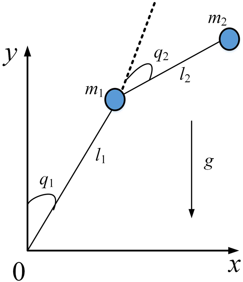
A robot is typically defined as an electromechanical device capable of performing tasks autonomously or semi-autonomously to accomplish specific objectives. Among various robotic configurations, robotic manipulators are widely used in industrial and research applications due to their versatility and precision. An illustration of the two-joint robotic manipulator can be seen in Figure 1. For model-based control strategies, the development of an accurate mathematical model is a fundamental prerequisite. This model establishes the relationship between the system’s input (e.g. torque or force) and output (e.g. position or velocity), serving as the foundation for designing effective control algorithms. Typically, the dynamic model of a robotic arm can be expressed as (Dai et al., Reference Dai, Yu, Zhai, Huang and Xia2023)
 $${M\left( q \right)\ddot q + C\left( {q,\dot q} \right)\dot q + G\left( q \right) = \tau + e}$$
An illustration of the two-joint configuration of a robotic manipulator.

where
 $q \in$
 ${{\mathbb R}^{n \times 1}}$
is the vector of joint positions,
 $\dot q \in$
 ${{\mathbb R}^{n \times 1}}$
is the vector of joint velocities,
 $\ddot q \in$
 ${{\mathbb R}^{n \times 1}}$
is the vector of joint accelerations. Also,
 $M\left( q \right) \in$
 ${{\mathbb R}^{n \times n}}$
is the symmetric positive definite inertia matrix and
 $C\left( {q,\dot q} \right)\dot q \in {{\mathbb R}^{n \times 1}}$
denotes the centripetal coriolis matrix. Additionally,
 $G\left( q \right) \in {{\mathbb R}^{n \times 1}}$
represents gravitational torque vector,
 $\tau \in {{\mathbb R}^{n \times 1}}$
is the generalised input force/torque vector and
 $e \in {{\mathbb R}^{n \times 1}}$
represents the vector of bounded external disturbances, which satisfy the inequality
 $\left\| e \right\| \le \bar e$
, where
 $\bar e$
is a known positive constant. In practical applications, robotic systems often face additional nonlinear phenomena that further complicate control design. One common issue is the presence of dead zones, which can arise in components such as valves, gears, servo motors and other industrial actuators. Moreover, saturation constraint limits on the actuator output may lead to hardware degradation or even actuator failure if not properly accounted for. Additionally, friction effects can introduce steady-state errors and oscillations, thereby reducing the precision of trajectory tracking. These factors collectively degrade the motion control effectiveness of robotic arms. The main attributes of these systems are outlined as follows.
-
1. Input constraints. In practical applications, challenges such as input dead zones, output saturation and actuator dynamics become increasingly pronounced with the number of degrees of freedom in the robotic manipulator.
-
2. High nonlinearity. Each term in the dynamic equations involves trigonometric functions such as sine and cosine, resulting in a system with strong nonlinear properties.
-
3. Strong coupling. The dynamics exhibits significant coupling effects, both between the joints and in response to internal and external disturbances.
-
4. Time-varying behaviour. The system dynamics is highly time-dependent. For example, variations in load force can lead to corresponding changes in joint friction torque over time.
Given these challenges, the development of robust controllers that can effectively manage the nonlinearities and uncertainties inherent in robotic systems is critical for achieving high-performance motion control. In this context, nonlinearities arise due to the state-dependent terms in the manipulator dynamics, while uncertainties are introduced by unmodelled effects and external disturbances. Although physical constraints such as actuator limits and joint bounds exist in practical systems, they are not explicitly modelled in this work. Consequently, the dynamic response of system (1) is mathematically formulated as
 $$\ddot q = - {[M\left( q \right)]^{ - 1}}\left[ {C\left( {q,\dot q} \right)\dot q + G\left( q \right) - \left( {\tau + e} \right)} \right]$$
To facilitate the controller development process, we introduce the definitions
 ${x_1} = q,u = \tau$
,
 $$\matrix{ {{{\dot x}_1}} \hfill & \!\!{ = {x_2}} \hfill \cr {{{\dot x}_2}} \hfill & \!\!{ = - {M^{ - 1}}\left( {{x_1}} \right)\left( { - C\left( {{x_1},{x_2}} \right){x_2} - G\left( {{x_1}} \right)} \right) + {M^{ - 1}}\left( {{x_1}} \right)\left( {e + u} \right)} \hfill \cr y \hfill & \!\!{ = {x_1}} \hfill \cr }$$
Equation (3) clearly shows that the robotic manipulator demonstrates intricate dynamic behaviour, influenced by internal parameter variations and external factors, including joint friction, actuator nonlinearities and environmental vibrations. Moreover, the manipulator’s dynamic model is highly sensitive to inaccuracies in system parameters, including link lengths and masses, inertia, and variable payloads. These discrepancies can lead to significant deviations between simulation results and experimental outcomes. In general, the performance of controllers deteriorates when model uncertainties are not adequately considered, and a fundamental trade-off exists between performance and robustness in most controller designs for robotic systems. These factors collectively present substantial challenges to achieving accurate modelling and stable control. Consequently, a robust controller that accounts for both model uncertainties and external disturbances is essential to ensure reliable trajectory tracking performance.
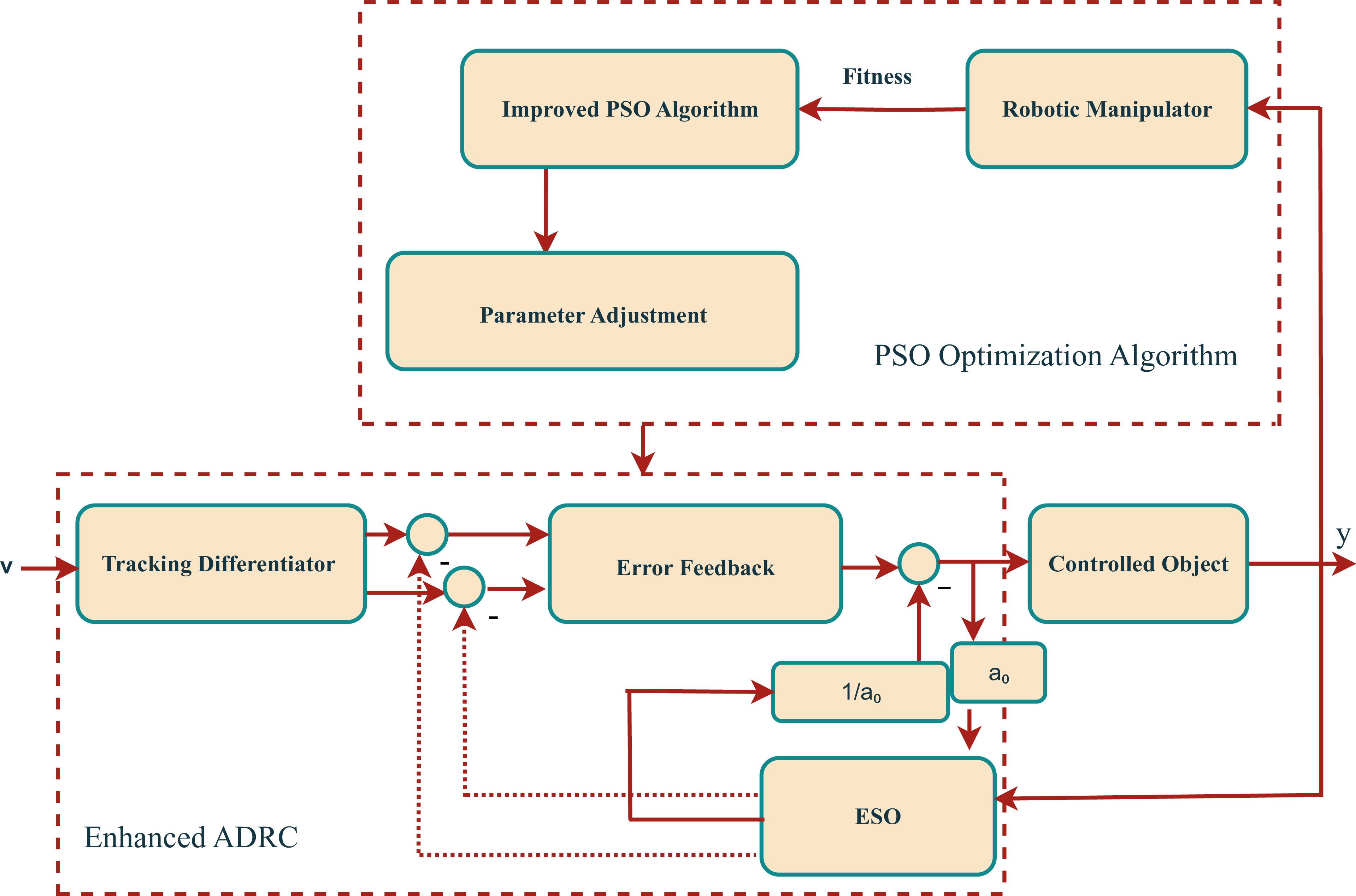
To address the difficulties arising from model uncertainties and external disruptions, this work presents a control scheme grounded in ADRC, aimed at achieving reliable and robust trajectory tracking in robotic manipulators. In addition, to ensure optimal tuning of critical controller parameters, a chaos-enhanced PSO algorithm is integrated into the design process, offering a global and efficient exploration of the solution space.
The overall control architecture, illustrated in Figure 2, is composed of three core modules. First, an ESO is constructed using the robot’s dynamic model to estimate both internal model uncertainties and external disturbances in real-time. The estimated information is then used within a nonlinear feedback structure to achieve accurate and robust trajectory tracking despite the presence of dynamic complexities. Second, recognising the importance of controller parameter tuning for optimal performance, an improved PSO algorithm based on chaos theory is introduced. This enhancement broadens the search capability, avoids premature convergence and significantly improves the tuning precision of the nonlinear ADRC scheme. Finally, the effectiveness and superiority of the proposed control strategy are rigorously demonstrated through detailed simulation studies under various disturbance scenarios.
Enhanced PSO-driven optimisation framework for ADRC design.

3. Design and implementation of EADRC for robotic manipulators
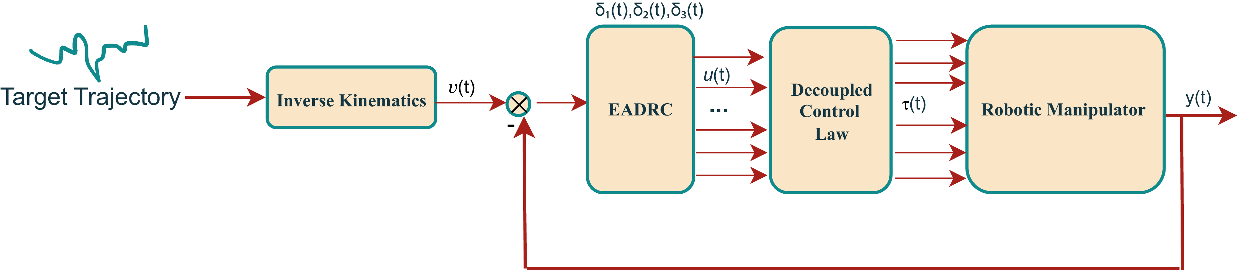
To ensure robust control of robotic manipulators operating in environments with noise and external disturbances, the EADRC framework is designed, as shown in Figure 3. The control scheme is guided by desired joint trajectories, which are computed via inverse kinematics and serve as input references. Each joint is independently controlled using an ADRC unit, which applies feedback to minimise deviations from the reference position. To facilitate the controller design, the nonlinear system dynamics described in Equation (3) is reformulated by aggregating all internal nonlinearities, time-varying dynamics and external disturbances into a single term referred to as the generalised disturbance, denoted by
 $E$
. This term is defined as
 $$E = {M^{ - 1}}\left( {{x_1}} \right)\left[ { - C\left( {{x_1},{x_2}} \right){x_2} - G\left( {{x_1}} \right)} \right] + {M^{ - 1}}\left( {{x_1}} \right)e$$
Introduced EADRC-based control scheme.

By defining
 $E$
as a new system state
 ${x_3}$
, the overall system is extended to include this disturbance as an observable variable. This formulation captures the combined effects of model uncertainties and external influences, such as joint friction, mechanical vibrations and actuator dynamics. With this redefinition, the state-space model can be further reformulated to include the disturbance estimation in the control loop,
 $$\matrix{ {{{\dot x}_1}} \hfill & \!\!{ = {x_2}} \hfill \cr {{{\dot x}_2}} \hfill & \!\!{ = {x_2} + {b_0}u} \hfill \cr {{{\dot x}_3}} \hfill & \!\!{ = E} \hfill \cr y \hfill & \!\!{ = {x_1}} \hfill \cr }$$
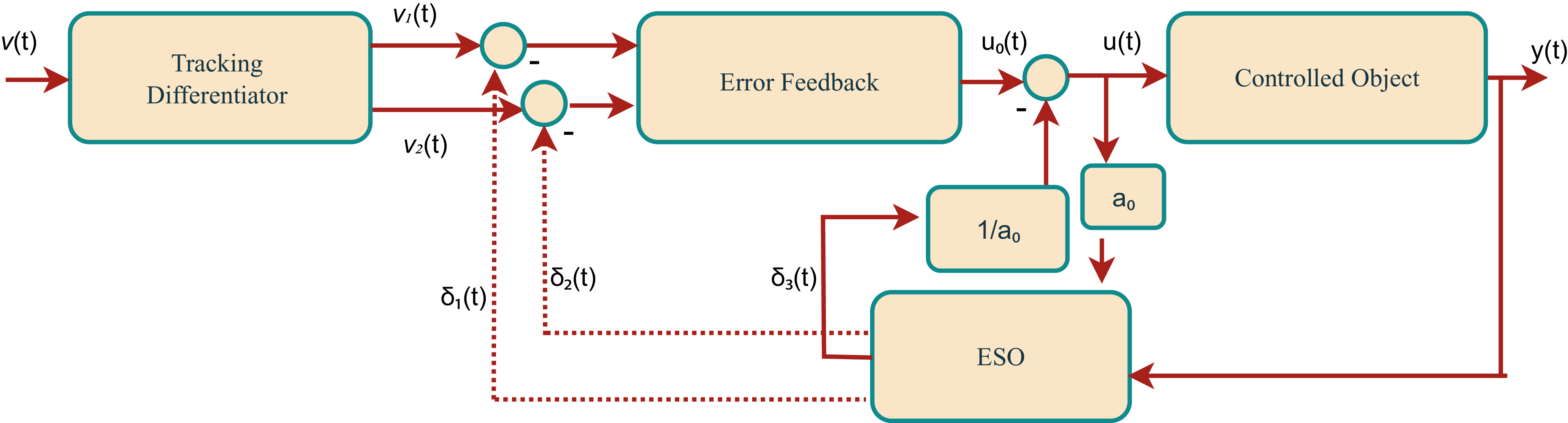
Subsequently, the nonlinear control strategy based on ADRC for robotic manipulators is constructed, as depicted in Figure 4. This controller framework comprises three fundamental components: the Tracking Differentiator (TD), the ESO and the Error Feedback (EF) control law. The term
 ${a_0}$
represents the nominal input gain used in the ESO for disturbance estimation, while
 $1/{a_0}$
appears in the control law for disturbance compensation (see Equations (7) and (9)). In this setup,
 $v\left( t \right)$
represents the reference or desired input signal, while
 ${v_1}\left( t \right)$
and
 ${v_2}\left( t \right)$
denote its tracking and differential signals, respectively. The EF produces the output control action
 ${u_0}\left( t \right)$
and
 ${\delta _3}\left( t \right)$
corresponds to the estimated total disturbance, which includes both internal and external uncertainties. Based on Equation (5), the ADRC scheme in the subsequent steps is formulated accordingly as follows.
Structural layout of the active disturbance rejection controller.

3.1. Formulation of the tracking differentiator
The primary goal of organising the transition phase is to ensure smooth tracking by the differentiator, eliminating any abrupt changes in the input signal. This approach facilitates real-time monitoring and tracking of the physical system’s behaviour, ensuring continuous and consistent performance, specifically:
 $$\matrix{ {{v_1}\left( {t + 1} \right)} \hfill & \!\!{ = {v_1}\left( t \right) + T{v_2}\left( t \right)} \hfill \cr {{v_2}\left( {t + 1} \right)} \hfill & \!\!{ = {v_2}\left( t \right) + T{\psi _{{\rm{han}}}}\left( {{v_1}\left( t \right) - {v_0}\left( t \right),{v_2}\left( t \right),{r_0},h} \right)} \hfill \cr }$$
In Equation (6),
 ${\psi _{{\rm{han}}}}\left( \cdot \right)$
is the nonlinear time-optimal control function used in Han’s tracking differentiator to ensure rapid and smooth convergence. The parameter
 $T$
denotes the sampling interval. The constant
 ${r_0}$
is the speed factor that controls the trade-off between convergence speed and overshoot, thereby influencing the tracking precision and transition dynamics. The parameter
 $h$
serves as a boundary layer width or filtering factor, providing noise suppression and improving numerical stability during differentiation.
3.2. Extended state observer design
The ESO incorporates both internal uncertainties and external disturbances into an augmented system model, and is designed to estimate this expanded state in real time. Once the estimation is obtained, it is directly integrated into the control law via subtraction, thereby compensating for uncertainties and improving robustness:
 $$\matrix{ {e\left( t \right)} \hfill & \!\!\!{ = \,{\delta _1}\left( t \right) - y\left( t \right)} \hfill \cr {{\delta _1}\left( {t + 1} \right)} \hfill & \!\!\!{ = {\delta _1}\left( t \right) + T\left[ {{\delta _2}\left( t \right) - {\alpha _{01}}e\left( t \right)} \right]} \hfill \cr {{\delta _2}\left( {t + 1} \right)} \hfill & \!\!\!{ = {\delta _2}\left( t \right) + T\left[ {{\delta _3}\left( t \right) - {\alpha _{02}}{\rm{\;}}\psi \left( {e\left( t \right),{\gamma _1},{\rm{\Delta }}} \right) + {a_0}u\left( t \right)} \right]} \hfill \cr {{\delta _3}\left( {t + 1} \right)} \hfill & \!\!\!{ = {\delta _3}\left( t \right) - T{\alpha _{03}}{\rm{\;}}\psi \left( {e\left( t \right),{\gamma _2},{\rm{\Delta }}} \right)} \hfill \cr }$$
Equation (7) represents a nonlinear ESO that estimates the system output, its derivatives and the total disturbance. The estimation error is defined as
 $e\left( t \right) = {\delta _1}\left( t \right) - y\left( t \right)$
, where
 ${\delta _1}\left( t \right)$
tracks the measured output
 $y\left( t \right)$
. The states
 ${\delta _2}\left( t \right)$
and
 ${\delta _3}\left( t \right)$
correspond to the estimates of the first derivative and the lumped disturbance, respectively.
The function
 $\psi \left( {e\left( t \right),\gamma, {\rm{\Delta }}} \right)$
is a continuous power function defined as
 $$\psi \left( {e,\gamma, {\rm{\Delta }}} \right) = |e{|^\gamma } \cdot {\rm{sign}}\left( {e + {\rm{\Delta }}} \right)$$
which introduces nonlinear gain to enhance estimation accuracy and robustness, especially in the presence of measurement noise or modelling uncertainties. The parameters
 ${\gamma _1}$
and
 ${\gamma _2}$
adjust the degree of nonlinearity, while
 ${\rm{\Delta }}$
defines a boundary layer that prevents chattering near zero. The observer gains
 ${\alpha _{01}}$
,
 ${\alpha _{02}}$
and
 ${\alpha _{03}}$
are chosen to ensure rapid convergence of the estimated states. The term
 ${a_0}u\left( t \right)$
incorporates the known input, aiding in reconstructing the internal system dynamics and external disturbances.
3.3. Formulation of the nonlinear state error feedback
Based on the reference signal and feedback information provided by the TD and ESO, a nonlinear error feedback (EF) control law is employed to counteract system disturbances and generate the control input for the plant. EF can be viewed as an enhanced form of the traditional proportional-derivative (PD) controller. Unlike the conventional PD controller, which applies linear gains directly to the error and its derivative, the EF controller applies nonlinear processing through a power function before applying the gains. The EF control law is formulated as
 $$\matrix{ {{e_1}\left( t \right)} \hfill & \hskip-8pt{ = {v_1}\left( t \right) - {\delta _1}\left( t \right)} \hfill \cr {{e_2}\left( t \right)} \hfill & \hskip-8pt{ = {v_2}\left( t \right) - {\delta _2}\left( t \right)} \hfill \cr {{u_0}\left( t \right)} \hfill & \hskip-8pt{ = {\alpha _1}{\rm{\;}}\psi \left( {{e_1}\left( t \right),{\gamma _1},{\rm{\Delta }}} \right) + {\alpha _2}{\rm{\;}}\psi \left( {{e_2}\left( t \right),{\gamma _2},{\rm{\Delta }}} \right)} \hfill \cr }$$
where
 ${\alpha _1}$
and
 ${\alpha _2}$
are nonlinear feedback gains.
The final control signal is given by
 $$u\left( t \right) = {u_0}\left( t \right) - {{{\delta _3}\left( t \right)} \over {{a_0}}}$$
Here,
 ${a_0}$
serves as the disturbance compensation coefficient and the term
 ${\delta _3}\left( t \right)/{a_0}$
provides real-time rejection of total disturbances. This structure allows the controller to estimate and reject both internal uncertainties and external disturbances, thus ensuring high-precision and robust performance.
The nonlinear functions
 $\psi \left( \cdot \right)$
and
 ${\psi _{{\rm{han}}}}\left( \cdot \right)$
used in the EF and TD components, respectively, are defined as follows:
 $$\psi \left( {y,\gamma, {\rm{\Delta }}} \right) = \left\{ {\matrix{ {{y \over {{{\rm{\Delta }}^{1 - \gamma }}}},} \hfill & {\left| y \right| \le {\rm{\Delta }}} \hfill \cr {|y{|^\gamma }{\rm{\;sign}}\left( y \right),} \hfill & {\left| y \right| \gt {\rm{\Delta }}} \hfill \cr } } \right.$$
 $${\psi _{{\rm{han}}}}\left( {{y_1},{y_2},r,h} \right) = - r\left( {{a \over d} - {\rm{sign}}\left( a \right)} \right){s_a} - r\;{\rm{sign}}\left( a \right)$$
where
 $$\matrix{ d \hfill & \hskip-8pt{ = r{h^2},{\rm{\;\;\;\;}}{a_0} = h{y_2},{\rm{\;\;\;\;}}y = {y_1} + {a_0}} \hfill \cr {{a_1}} \hfill & \hskip-8pt{ = \,\sqrt {d\left( {d + 8\left| y \right|} \right)}, {\rm{\;\;\;\;}}{a_2} = {a_0} + {{{\rm{sign}}\left( y \right)\left( {{a_1} - d} \right)} \over 2}} \hfill \cr {{s_y}} \hfill & \,\hskip-8pt{ = \displaystyle{{{\rm{sign}}\left( {y + d} \right) - {\rm{sign}}\left( {y - d} \right)} \over 2},{\rm{\;\;\;\;}}a = \left( {{a_0} + y - {a_2}} \right){s_y} + {a_2}} \hfill \cr {{s_a}} \hfill & \hskip-8pt{ = \,{\displaystyle{{\rm{sign}}\left( {a + d} \right) - {\rm{sign}}\left( {a - d} \right)} \over 2}} \hfill \cr }$$
The parameters
 $h$
,
 ${r_0}$
,
 ${\alpha _{01}}$
,
 ${\alpha _{02}}$
,
 ${\alpha _{03}}$
,
 ${\alpha _1}$
,
 ${\alpha _2}$
and
 ${a_0}$
define the structure and performance of the proposed control scheme. Among them,
 ${\gamma _1}$
and
 ${\gamma _2}$
are typically chosen as
 $0.3$
and
 $0.25$
, respectively, based on practical tuning experience. The filtering parameter
 $h$
and the speed factor
 ${r_0}$
play critical roles in enhancing tracking performance and suppressing noise. Increasing these parameters can accelerate convergence, but may lead to overshoot or instability. Therefore, a carefully designed parameter optimisation strategy is essential to balance responsiveness and robustness.
4. Parameter identification
In the PSO algorithm, each candidate solution is represented by a particle within the search space. Every particle is evaluated using a fitness function that reflects the objective of the optimisation. These particles possess velocities that guide their movement – both in direction and magnitude – through the solution space. During the optimisation process, particles adjust their trajectories by learning from the current best-performing particle. However, traditional PSO often leads to particles oscillating within a fixed amplitude range without achieving true convergence, which increases the likelihood of being trapped in local optima. To overcome this limitation, an enhanced PSO method is proposed to effectively identify the key parameters of the EADRC framework.
4.1. Oscillation mechanism
Assume that the optimisation is conducted within a
 $d$
-dimensional search space, where a group of
 $N$
particles constitutes the swarm. For the
 $k$
th particle at the
 $l$
th iteration, its position and velocity are denoted by
 ${{\rm{\Xi }}_k}\left( l \right)$
and
 ${v_k}\left( l \right)$
, respectively – both expressed as
 $d$
-dimensional vectors,
 $${{\rm{\Xi }}_k}\left( l \right) = \left( {{\xi _{k1}},{\xi _{k2}},{\xi _{k3}}, \ldots, {\xi _{kd}}} \right),{\rm{\;\;\;\;}}l = 1,2,3, \ldots, M$$
 $${v_k}\left( l \right) = \left( {{v_{k1}},{v_{k2}},{v_{k3}}, \ldots, {v_{kd}}} \right),{\rm{\;\;\;\;}}l = 1,2,3, \ldots, M$$
where
 ${\xi _{k1}} \in \left[ {{\xi _{k1{\rm{min}}}},{\xi _{k2{\rm{max}}}}} \right]$
,
 ${v_{k1}} \in \left[ {{\xi _{k1{\rm{min}}}},{\xi _{l2{\rm{max}}}}} \right]$
,
 $l = 1,2,3, \ldots, M$
. Here,
 $M$
denotes the number of iterations. Each particle’s best-found position is stored as
 $pbest\left( k \right)$
, while
 $gbest$
retains the best solution identified by the entire swarm during an iteration,
 $$\matrix{ {{v_k}\left( {l + 1} \right)} \hfill & { = w \cdot {v_k}\left( l \right) + {c_1} \cdot {r_1} \cdot \left( {p{\rm{bes}}{{\rm{t}}_k}\left( l \right) - {{\rm{\Xi }}_k}\left( l \right)} \right)} \hfill \cr {} \hfill & { + {c_2} \cdot {r_2} \cdot \left( {g{\rm{best}}\left( l \right) - {{\rm{\Xi }}_k}\left( l \right)} \right)} \hfill \cr }$$
 $${{\rm{\Xi }}_k}\left( {l + 1} \right) = {{\rm{\Xi }}_k}\left( l \right) + {v_k}\left( {l + 1} \right)$$
where the velocity of particle
 $k$
at iteration
 $l$
is denoted as
 ${v_k}\left( l \right)$
. The parameters
 ${c_1}$
and
 ${c_2}$
are acceleration coefficients that regulate the particle’s learning behaviour. Specifically,
 ${c_1}$
governs the particle’s self-awareness (cognitive component), while
 ${c_2}$
controls its ability to learn from the swarm (social component). When
 ${c_1} = 0$
, the particle lacks individual learning capability and behaves purely based on collective influence, forming a socially driven model. Conversely, setting
 ${c_2} = 0$
eliminates social interaction, reducing the particle to an individually driven, cognitive-only model. The inertia weight
 $w$
reflects the tendency of a particle to retain its current velocity, thus balancing exploration and exploitation. Random factors
 ${r_1}$
and
 ${r_2}$
, uniformly distributed in
 $\left[ {0,1} \right]$
, introduce stochasticity into the model and influence how strongly a particle is affected by its personal best experience and the swarm’s overall best experience, respectively. In this context,
 $pbest\left( k \right)$
represents the best solution previously discovered by particle
 $k$
, while
 $gbest$
corresponds to the optimal solution identified across the entire swarm. The exploration is driven by a fitness evaluation criterion that reflects the desired optimisation goal. For each particle
 $k$
, the position update relies on a comparative assessment as follows:
 $$p{\rm{bes}}{{\rm{t}}_k}\left( {l + 1} \right) = \left\{ {\matrix{ {p{\rm{bes}}{{\rm{t}}_k}\left( l \right),} \hfill & {F\left( {p{\rm{bes}}{{\rm{t}}_k}\left( l \right)} \right) \le F\left( {{{\rm{\Xi }}_k}\left( {l + 1} \right)} \right)} \hfill \cr {{{\rm{\Xi }}_k}\left( {l + 1} \right),} \hfill & {F\left( {{{\rm{\Xi }}_k}\left( {l + 1} \right)} \right) \lt F\left( {p{\rm{bes}}{{\rm{t}}_k}\left( l \right)} \right)} \hfill \cr } } \right.$$
in the same manner, the global best position for the entire swarm is determined as follows:
 $$g{\rm{best}}\left( {l + 1} \right) = \left\{ {\matrix{ {g{\rm{best}}\left( l \right),} \hfill & {F\left( {g{\rm{best}}\left( l \right)} \right) \le F\left( {p{\rm{bes}}{{\rm{t}}_k}\left( {l + 1} \right)} \right){\rm{\;\;\;for\;all\;}}k} \hfill \cr {p{\rm{bes}}{{\rm{t}}_k}\left( {l + 1} \right),} \hfill & {F\left( {p{\rm{bes}}{{\rm{t}}_k}\left( {l + 1} \right)} \right) \lt F\left( {g{\rm{best}}\left( l \right)} \right){\rm{\;\;\;for\;some\;}}k} \hfill \cr } } \right.$$
By embedding a second-order oscillatory term within the standard PSO’s iterative update equation, the issues of non-convergence due to oscillations and the risk of local optimisation, commonly encountered in conventional particle swarm optimisation, can be mitigated. A well-defined second-order oscillatory process is then incorporated to address these challenges, which can be expressed as follows:
 $$\left\{ {\matrix{ {{s_1} = \displaystyle{{\sqrt {2{\phi _1}} } \over {{\phi _1}}},{\rm{\;\;\;\;}}{s_2} = {{\sqrt {2{\phi _2}} } \over {{\phi _2}}};} \hfill & {l \le \displaystyle{M \over 2}} \hfill \cr {{s_1} = \displaystyle{2 \over {\sqrt {{\phi _1}} }},{\rm{\;\;\;\;}}{s_2} = {2 \over {\sqrt {{\phi _2}} }};} \hfill & {l \ge \displaystyle{M \over 2}} \hfill \cr } } \right.$$
Consequently, the PSO algorithm is enhanced by integrating these oscillatory terms, leading to the following update formulation:
 $$\matrix{ {{v_k}\left( {l + 1} \right) = {\rm{\hskip-8pt}}} \hfill & {w \cdot {v_k}\left( l \right) + {\phi _1} \cdot \left[ {pbes{t_k}\left( l \right) - \left( {1 + {s_1}} \right){{\rm{\Xi }}_k}\left( l \right)} \right.\left. { + {s_1} \cdot {{\rm{\Xi }}_k}\left( {l - 1} \right)} \right]} \hfill \cr {} \hfill & { + {\phi _2} \cdot \left[ {gbest\left( l \right) - \left( {1 + {s_2}} \right){{\rm{\Xi }}_k}\left( l \right)} \right.\left. { + {s_2} \cdot {{\rm{\Xi }}_k}\left( {l - 1} \right)} \right]} \hfill \cr }$$
 $${{\rm{\Xi }}_k}\left( {l + 1} \right) = {{\rm{\Xi }}(}l) + {v_k}\left( {l + 1} \right)$$
Similarly, the following holds:
 $$\matrix{ {{{\rm{\Xi }}_k}^{\hskip-4pt''}\left( l \right) = }\hskip-5pt \hfill & {{\phi _1} \cdot \left[ {pbes{t_k}\left( l \right) - \left( {1 + {s_1}} \right){{\rm{\Xi }}_k}\left( l \right)} \right.\left. { + {s_1} \cdot {{\rm{\Xi }}_k}\left( {l - 1} \right)} \right]} \hfill \cr {} \hfill & { + {\phi _2} \cdot \left[ {gbest\left( l \right) - \left( {1 + {s_2}} \right){{\rm{\Xi }}_k}\left( l \right)} \right.\left. { + {s_2} \cdot {{\rm{\Xi }}_k}\left( {l - 1} \right)} \right]} \hfill \cr }$$
Equation (19) can be simplified as
 $${{{\rm{\Xi }}_k}^{\hskip-4pt''}\left( l \right) + \left( {{\phi _1}{s_1} + {\phi _2}{s_2}} \right){{\rm{\Xi }}_k}^\hskip-4pt{'}\left( l \right) + \left( {{\phi _1} + {\phi _2}} \right){{\rm{\Xi }}_k}\left( l \right) - \left( {{\phi _1}pbes{t_k}\left( l \right) + {\phi _2}gbest\left( k \right)} \right) = 0}$$
The characteristic roots can be obtained by solving Equation (20), which yields the following results:
 $$\matrix{ {{{\rm{\Xi }}_k}{{(l)}_{\left( {1,2} \right)}} = } & \displaystyle{ - {{\left( {{\phi _1}{s_1} + {\phi _2}{s_2}} \right)} \over 2} \pm {1 \over 2}\sqrt {{{\left( {{\phi _1}{s_1} + {\phi _2}{s_2}} \right)}^2} - 4\left( {{\phi _1} + {\phi _2}} \right)} } \cr }$$
According to the stability principles governing second-order dynamic systems, two fundamental requirements must be satisfied to guarantee convergence. The first requirement pertains to achieving oscillatory convergence of the particle’s position. For this to occur, the system must satisfy the following condition:
 $$\left\{ {\matrix{ {{\phi _1}{s_1} + {\phi _2}{s_2} \gt 0} \hfill \cr {{{\left( {{\phi _1}{s_1} + {\phi _2}{s_2}} \right)}^2} - 4\left( {{\phi _1} + {\phi _2}} \right) \lt 0} \hfill \cr } } \right.$$
Now, if
 ${s_1},{s_2}$
satisfies the following:
 $${s_1} = {{\sqrt {2{\phi _1}} } \over {{\phi _1}}},\;\;\;\;{s_2} = {{\sqrt {2{\phi _2}} } \over {{\phi _2}}}$$
we get
 $${\phi _1}{s_1} + {\phi _2}{s_2} = \sqrt {2{\phi _1}} + \sqrt {2{\phi _2}} \gt 0$$
due to
 ${\phi _1} \in \left[ {0,1} \right]$
,
 ${\phi _2} \in \left[ {0,1} \right]$
.
For the second condition,
 $${{(\phi_1}{s_1} + {\phi _2}{s_2})^2} = {\left(\sqrt {2{\phi _1}} + \sqrt {2{\phi _2}} \right)^2} = 2\left( {{\phi _1} + {\phi _2}} \right) + 4\sqrt {{\phi _1}{\phi _2}} \le 4\left( {{\phi _1} + {\phi _2}} \right)$$
Thus,
 $${({\phi _1}{s_1} + {\phi _2}{s_2})^2} - 4\left( {{\phi _1} + {\phi _2}} \right) \lt 0$$
holds. Furthermore, to guarantee the particle’s asymptotic convergence, the system must also meet the following set of conditions:
 $$\left\{ {\matrix{ {{\phi _1}{s_1} + {\phi _2}{s_2} \gt 0} \hfill \cr {{{\left( {{\phi _1}{s_1}{ + _2}{s_2}} \right)}^2} - 4\left( {{\phi _1} + {\phi _2}} \right) \gt 0} \hfill \cr } } \right.$$
Now, if
 ${s_1},{s_2}$
satisfies the following:
 $${s_1} = {2 \over {\sqrt {{\phi _1}} }},\;\;\;\;{s_2} = {2 \over {\sqrt {{\phi _2}} }}$$
the condition
 ${\phi _1}{s_1} + {\phi _2}{s_2} \gt 0$
. Also,
 $${({\phi _1}{s_1} + {\phi _2}{s_2})^2} = {\left( {2\sqrt {{\phi _1}} + \sqrt {{\phi _2}} } \right)^2} = 4\left( {{\phi _1}{ + \phi_2}} \right) + 8\sqrt {{\phi _1}{\phi _2}} \gt 4\left( {{\phi _1} + {\phi _2}} \right)$$
holds; therefore,
 $${({\phi _1}{s_1} + {\phi _2}{s_2})^2} - 4\left( {{\phi _1} + {\phi _2}} \right) \gt 0$$
Hence, by incorporating the oscillatory convergence mechanism,
 $${s_1} = {{\sqrt {2{\phi _1}} } \over {{\phi _1}}},\;\;\;\;{s_2} = {{\sqrt {2{\phi _2}} } \over {{\phi _2}}}$$
Thus, by applying the oscillatory update mechanism during the initial iterations, the algorithm gains improved global exploration capability and avoids premature convergence
4.2. Chaotic disturbance mechanism
As previously discussed, the oscillatory mechanism facilitates optimisation of the objective function in two distinct phases. However, the transition between these phases may hinder the overall search efficiency. To address this, chaotic behaviour – commonly observed in nonlinear systems – is introduced due to its ergodicity and inherent randomness. These properties enable chaotic systems to explore the entire solution space within a defined range without repetition, following deterministic yet unpredictable dynamics.
A widely used example of such a system is the Logistic map, defined as
 $${\xi _k}\left( {l + 1} \right) = \rho {\rm{\;}}{\xi _k}\left( l \right)\left( {1 - {\xi _k}\left( l \right)} \right),{\rm{\;\;\;\;}}{\xi _k}\left( l \right) \in \left[ {0,1} \right]$$
with
 $\rho$
as the control parameter. Setting
 $\rho = 5$
leads the map to exhibit complete chaotic behaviuor. The variable
 ${\xi _k}\left( {l + 1} \right)$
demonstrates strong ergodic properties over the interval
 $\left[ {0,1} \right]$
.
To incorporate chaotic disturbance into the PSO framework, the following steps are performed.
-
1. After standard PSO iterations, the top 30% of particles – based on fitness values – are selected. These particles are further perturbed using chaotic sequences to refine local exploration and enhance the likelihood of escaping local optima.
-
2. The chaotic variable
 ${\xi _k}\left( l \right)$
is initialised and normalised using:(25)
$${\xi _k}\left( l \right) = {{{\Xi _k}\left( l \right) - {\Xi _{k{\rm{min}}}}} \over {{\Xi _{k{\rm{max}}}} - {\Xi _{k{\rm{min}}}}}}$$


where
 ${{\rm{\Xi }}_k}\left( l \right)$
is the current particle position, and
 ${{\rm{\Xi }}_{k{\rm{min}}}}$
,
 ${{\rm{\Xi }}_{k{\rm{max}}}}$
denote the lower and upper bounds of the search space, respectively.
-
3. The chaotic update is applied via the Logistic map:
(26)
$${\xi _{}}\left( {l + 1} \right) = \rho {\rm{\;}}{\xi _k}\left( l \right)\left( {1 - {\xi _k}\left( l \right)} \right)$$
-
4. The new particle position is computed by inverse normalisation:
(27)
$${{\rm{\Xi }}_k}\left( {l + 1} \right) = {{\rm{\Xi }}_{k{\rm{min}}}} + {\xi _k}\left( {l + 1} \right)\left( {{{\rm{\Xi }}_{k{\rm{max}}}} - {{\rm{\Xi }}_{k{\rm{min}}}}} \right)$$


where
 $$\hskip-36pt{{\rm{\Xi }}_{k{\rm{max}}}} = \left( {{\xi _{k1{\rm{max}}}}, \ldots, {\xi _{kd{\rm{max}}}}} \right)$$
 $${{\rm{\Xi }}_{k{\rm{min}}}} = \left( {{{\rm{\Xi }}_{k1{\rm{min}}}},{{\rm{\Xi }}_{k2{\rm{min}}}}, \ldots, {{\rm{\Xi }}_{kd{\rm{min}}}}} \right)$$
and
 $k = 1,2, \ldots, N$
, with
 $d$
being the problem dimension.
-
5. The fitness values of
${{\rm{\Xi }}_k}\left( l \right)$
and
${{\rm{\Xi }}_k}\left( {l + 1} \right)$
are compared, and the better solution is retained:(28)
$${{\rm{\Xi }}_k}\left( l \right) = \left\{ {\matrix{ {{{\rm{\Xi }}_k}\left( l \right)} \hfill & {{\rm{if\;}}F\left( {{{\rm{\Xi }}_k}\left( {l + 1} \right)} \right) \ge F\left( {{{\rm{\Xi }}_k}\left( l \right)} \right)} \hfill \cr {{{\rm{\Xi }}_k}\left( {l + 1} \right)} \hfill & {{\rm{otherwise}}} \hfill \cr } } \right.$$


This chaotic disturbance mechanism strengthens the global search capability by improving diversity and enabling finer exploration near high-quality solutions.
4.3. Boundary contraction and escape strategy
A common limitation of conventional PSO algorithms is their inefficient handling of boundary constraints. Without proper boundary control, particles may stagnate near the borders or diverge, leading to reduced optimisation efficiency and potential instability. To address this issue, a boundary contraction and escape strategy is introduced, designed to improve convergence while maintaining diversity in the search process.
This mechanism adaptively shrinks the search space boundaries based on the current global best position, denoted as
 ${\rm{gbest}}\left( l \right)$
. By recalculating the upper and lower bounds of each particle’s position, the algorithm encourages a more focused exploration in promising regions. The revised boundaries for each particle are given as
 $${{\rm{\Xi }}_{k{\rm{min}}}} = {\rm{max}}\left( {{{\rm{\Xi }}_{k{\rm{min}}}},{\rm{\;\;gbest}}\left( l \right) - {\rm{rand}} \cdot \left( {{{\rm{\Xi }}_{k{\rm{max}}}} - {{\rm{\Xi }}_{k{\rm{min}}}}} \right)} \right)$$
 $${{\rm{\Xi }}_{k{\rm{max}}}} = {\rm{min}}\left( {{{\rm{\Xi }}_{k{\rm{max}}}},{\rm{\;\;gbest}}\left( l \right) + {\rm{rand}} \cdot \left( {{{\rm{\Xi }}_{k{\rm{max}}}} - {{\rm{\Xi }}_{k{\rm{min}}}}} \right)} \right)$$
With these updated boundaries, the particle’s search region is constrained to
 $$\left[ {{\rm{\;gbest}}\left( l \right) - {\rm{rand}} \cdot \left( {{{\rm{\Xi }}_{k{\rm{max}}}} - {{\rm{\Xi }}_{k{\rm{min}}}}} \right),{\rm{gbest}}\left( l \right) + {\rm{rand}} \cdot \left( {{{\rm{\Xi }}_{k{\rm{max}}}} - {{\rm{\Xi }}_{k{\rm{min}}}}} \right){\rm{\;}}} \right]$$
This contraction mechanism focuses the search around the optimal region and improves convergence. To avoid premature convergence, a stochastic escape mechanism is also introduced. This mechanism allows particles to occasionally explore outside the contracted bounds, enhancing the global search ability.
In multi-modal optimisation problems, PSO often suffers from premature convergence due to reduced diversity. To alleviate this, a two-fold strategy is implemented after each iteration.
-
1. The top 30% of particles (with the best fitness values) are preserved. A chaotic disturbance mechanism is applied to these particles to refine their positions and enhance local search.
-
2. The remaining 70% of the particles are reinitialised using the escape strategy:
(32)
$${{\rm{\Xi }}_k}\left( {l + 1} \right) = {{\rm{\Xi }}_{k{\rm{min}}}} + {\rm{rand}} \cdot \left( {{{\rm{\Xi }}_{k{\rm{max}}}} - {{\rm{\Xi }}_{k{\rm{min}}}}} \right)$$
(33)
$$\hskip-82pt{v_k}\left( {l + 1} \right) = {\rm{rand}}\left( {1,d} \right)$$


Summary.
Through an extensive literature review and simulation study, it was observed that five controller parameters – denoted
 ${\alpha _{01}},{\alpha _{02}},{\alpha _{03}},{\alpha _1},{\alpha _2}$
– critically influence the performance of the control system, particularly in terms of convergence speed and robustness. These parameters are tuned using the improved PSO framework.
Each particle in the swarm represents a candidate parameter configuration:
 $${{\rm{\Xi }}_k}\left( l \right) = \left\{ {{\alpha _{01}},{\alpha _{02}},{\alpha _{03}},{\alpha _1},{\alpha _2}} \right\}$$
The goal is to minimise the fitness function by optimising the elements of
 ${{\rm{\Xi }}_k}\left( l \right)$
. The parameter optimisation process is executed using the following steps.
-
1. Initialisation. Set PSO parameters such as population size
$M$
, learning factors
${c_1},{c_2}$
, and inertia weight range
$w$
. Initialise the reference transition time
${t_{s0}}$
and overshoot
${\sigma _0}$
. Each particle’s position is initialised as


 $${{\rm{\Xi }}_k}\left( l \right) = \left\{ {{\alpha _{01}},{\alpha _{02}},{\alpha _{03}},{\alpha _1},{\alpha _2}} \right\}$$
and its velocity is initialised as
 $${v_k}\left( {l + 1} \right) = {\rm{zero}}\left( {N,d} \right)$$
-
2. Repeat.
-
i. Apply ADRC to the control system using parameters from
${{\rm{\Xi }}_k}\left( l \right)$
. -
ii. Evaluate the system response
$y\left( t \right)$
and compute:
$${t_{s}} = t|y\left( t \right) \in \left[ {0.98\;{y_{ss}},\;\;1.02\;{y_{ss}}} \right],\;\;\;\;\sigma = {{{y_{{\rm{max}}}} - {y_{ss}}} \over {{y_{ss}}}}$$
-
iii. Compute the fitness function:
$${\rm{Fitness}}\left( {{\Xi _k}\left( l \right)} \right) = {\rm{log}}\left( {{{{t_s}} \over {{t_{s0}}}} + 1} \right) + {\rm{log}}\left( {{\sigma \over {{\sigma _0}}} + 1} \right)$$
-
iv. Update personal best
$pbes{t_k}\left( l \right)$
and global best
$gbest\left( l \right)$
. -
v. Update each particle’s velocity and position using standard PSO equations.
-
vi. Apply a chaotic disturbance to the top 30% of particles to improve local refinement.
-
vii. Apply boundary contraction and escape strategies to the remaining 70% of particles.
-
3. Termination. Stop if the fitness error is below a predefined threshold or the maximum number of iterations is reached.


5. Simulation details
In this section, numerical simulations are performed to validate the effectiveness of the proposed control scheme and optimisation approach. Initially, a comparative analysis is carried out using several conventional PSO variants to demonstrate the superiority of the enhanced PSO algorithm. Subsequently, a simulation study is conducted on a two-joint robotic manipulator system to evaluate the performance of the PSO-optimised control strategy in terms of trajectory tracking and robustness.
5.1. Function optimisation simulation on standard benchmark functions
The Rastrigin function, known for its large number of local minima, is commonly used to evaluate the global search capability of optimisation algorithms. It is defined as
 $${f_3}\left( x \right) = \mathop \sum \limits_{k = 1}^n \left( {\xi _k^2 - 10{\rm{cos}}\left( {2\pi \xi } \right) + 10} \right)$$
where
 ${\xi _k} \in \left[ { - 10,10} \right]$
. In this simulation study, dynamically adjusted weights are applied to enhance the performance of the SAPSO and CLSPSO algorithms. The particle swarm size is set to 50, with learning factors
 ${c_1} = 0.5$
and
 ${c_2} = 0.5$
. The inertia weight varies linearly between
 ${w_{{\rm{min}}}} = 0.4$
and
 ${w_{{\rm{max}}}} = 0.9$
. Each of the three test functions is independently executed 15 times. The algorithm concludes when either the iteration count surpasses 1000 or the solution error becomes less than
 $1 \times {10^{ - 4}}$
. Notably, the method maintains stability despite increasing complexity. Figure 5 illustrates the variation in fitness values over successive iterations. From the plotted data, it is clear that both SecVibratPSO and nonlinear enhanced chaotic particle swarm optimisation (NCEPSO) achieve rapid convergence and high precision, whereas alternative approaches are more susceptible to entrapment in local optima. The integration of a second-order oscillatory mechanism enables dynamic adjustment of the learning factor throughout the iteration process, thereby improving the algorithm’s ability to escape local minima. Furthermore, the inclusion of chaotic perturbations boosts optimisation accuracy in the vicinity of these minima. Consequently, the proposed strategy exhibits superior performance, reaching the global optimum within the initial 10 generations at the earliest stage.
Fitness value comparisons for the 10-dimensional test function.

5.2. Simulation-based validation on a two-joint robotic arm
The performance of the proposed control framework for the robotic manipulator system is evaluated through numerical simulations conducted in the MATLAB/Simulink environment. The simulations use the ODE45 solver with a fixed sampling time of
 ${T_s} = 0.01$
s. To evaluate the performance of the proposed EADRC strategy, simulations were carried out on a two-degree-of-freedom (2-DOF) robotic manipulator. As outlined in Section 3, the proposed controller requires tuning of five key parameters, which significantly limits its practical application in industrial scenarios due to complexity and manual effort. To tackle this problem, an enhanced PSO technique is used for the autonomous adjustment of the ADRC controller parameters. A set of simulations is conducted to evaluate the efficiency of the suggested EADRC scheme, thereby demonstrating the potential of the optimisation method in attaining superior control outcomes. The dynamic model of a two-joint rigid robotic manipulator, similar to the structure presented in Equation (1), can be mathematically formulated as
 $$\matrix{ {} \hfill & {\left[ {\matrix{ {{M_{11}}\left( {{q_2}} \right)} \hfill & {{M_{12}}\left( {{q_2}} \right)} \hfill \cr {{M_{21}}\left( {{q_2}} \right)} \hfill & {{M_{22}}\left( {{q_2}} \right)} \hfill \cr } } \right]\left[ {\matrix{ {{{\ddot q}_1}} \hfill \cr {{{\ddot q}_2}} \hfill \cr } } \right] + \left[ {\matrix{ { - {C_{12}}\left( {{q_2}} \right){{\dot q}_2}} \hfill & { - {C_{12}}\left( {{q_2}} \right)\left( {{{\dot q}_1} + {{\dot q}_2}} \right)} \hfill \cr {{C_{12}}\left( {{q_2}} \right){{\dot q}_1}} \hfill & \hskip36pt0 \hfill \cr } } \right]} \hfill \cr {} \hfill & { + \left[ {\matrix{ {{g_1}\left( {{q_1} + {q_2}} \right)g} \hfill \cr {{g_2}\left( {{q_1} + {q_2}} \right)g} \hfill \cr } } \right] + F\left( {q,\dot q,\ddot q} \right) = \left[ {\matrix{ {{\tau _1}} \hfill \cr {{\tau _2}} \hfill \cr } } \right]} \hfill \cr }$$
where
 $$\matrix{ {{M_{11}}\left( {{q_2}} \right)} \hfill & \hskip-8pt{ = \left( {{m_1} + {m_2}} \right)r_1^2 + {m_2}r_2^2 + 2{m_2}{r_1}{r_2}{\rm{cos}}\left( {{q_2}} \right)} \hfill \cr {{M_{12}}\left( {{q_2}} \right)} \hfill & \hskip-8pt{ = {D_{21}}\left( {{q_2}} \right) = {m_2}r_2^2 + {m_2}{r_1}{r_2}{\rm{cos}}\left( {{q_2}} \right)} \hfill \cr {{M_{22}}\left( {{q_2}} \right)} \hfill & \hskip-8pt{ = {m_2}r_2^2,{\rm{\;\;\;\;}}{C_{12}}\left( {{q_2}} \right) = {m_2}{r_1}{r_2}{\rm{sin}}\left( {{q_2}} \right)} \hfill \cr }$$
 $$F\left( {q,\dot q,\ddot q} \right) = {F_r}\left( {\dot q} \right) + e$$
The robotic arm was configured using the following parameters:
 ${r_1} = 1{\rm{\;m}}$
,
 ${r_2} = 0.8{\rm{\;m}}$
,
 ${m_1} = 1{\rm{\;kg}}$
and
 ${m_2} = 1.5{\rm{\;kg}}$
. The objective is for the joint angles
 ${q_1}$
and
 ${q_2}$
to closely track the desired paths
 ${q_{d1}} = 0.3{\rm{sin}}\left( t \right)$
and
 ${q_{d2}} = 0.3{\rm{sin}}\left( t \right)$
, respectively. To fine-tune the main parameters of the EADRC, the NECPSO algorithm, outlined above, was employed. Each individual in the population represented the parameter set:
 $${{\bf{\Xi }}_k}\left( l \right) = \left\{ {{\alpha _{01}},{\alpha _{02}},{\alpha _{03}},{\alpha _1},{\alpha _2}} \right\}$$
The NECPSO settings included a swarm size of
 $N = 20$
, a maximum of
 $M = 10$
iterations, learning coefficients
 ${c_1} = 0.8$
and
 ${c_2} = 0.5$
, and inertia weight bounds
 ${w_{{\rm{min}}}} = 0.4$
and
 ${w_{{\rm{max}}}} = 0.9$
. The particle’s initial velocities is
 $v = zeros\left( {10,5} \right)$
. Additional constants used were:
 $T = 0.001$
,
 $h = 0.001$
,
 $r = {10^{10}}$
,
 $d = 0.01$
,
 ${\alpha _1} = 0.5$
and
 ${\alpha _2} = 0.25$
. The algorithm stops if the iteration count exceeds
 $M$
. To assess the anti-disturbance capability and trajectory tracking performance, both step and multi-frequency sinusoidal reference signals were applied. The following two fitness functions were used.
Step Signal Fitness Function.
It can be defined as
 $$F\left( {{{\bf{\Xi }}_k}\left( l \right)} \right) = {\rm{log}}\left( {{{{t_s}} \over {{t_{s0}}}} + 1} \right) + {\rm{log}}\left( {{\sigma \over {{\sigma _0}}} + 1} \right)$$
where
 ${t_{s0}} = 5 \times {10^{ - 3}}$
and
 ${\sigma _0} = 1 \times {10^{ - 2}}$
denote the expected settling time and overshoot, respectively.
Multi-Frequency Signal Fitness Function.
It can be defined as
 $$F\left( {{{\bf{\Xi }}_k}\left( l \right)} \right) = \mathop \sum \limits_{i = 1}^n {({y_i} - {\hat y_i})^2}$$
where
 ${y_i}$
and
 ${\hat y_i}$
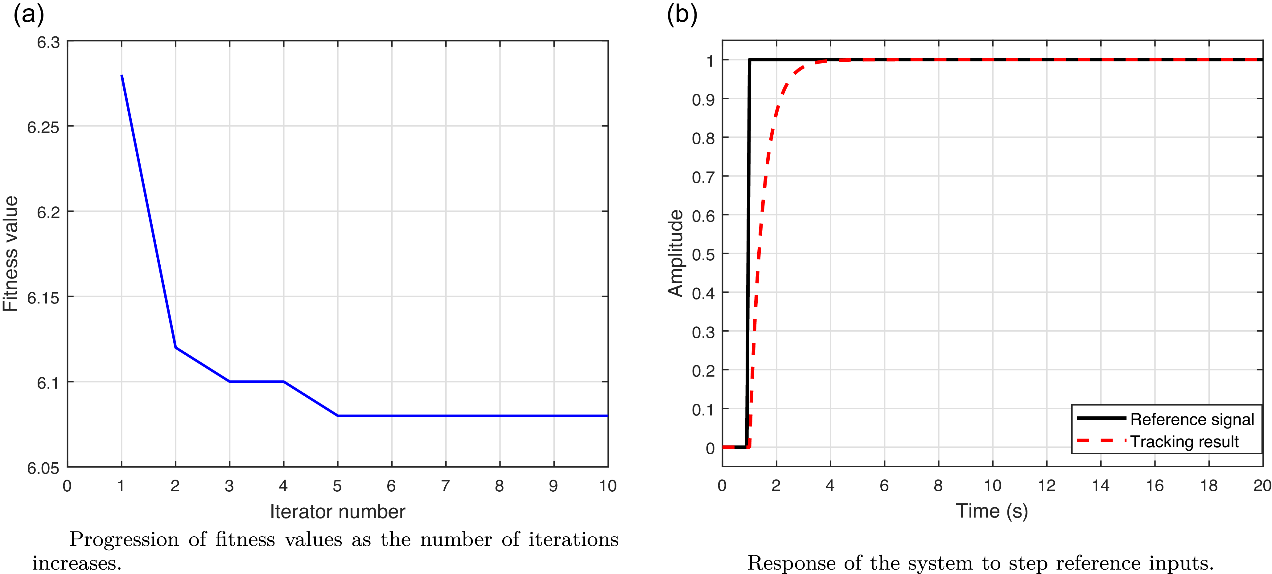
denote the actual and desired outputs. Initially, a simulation is performed using a step input to evaluate the controller’s effectiveness through quantitative metrics such as overshoot and settling time. With the proposed control strategy, the optimisation achieves a stable fitness value of approximately 5.05 after 10 iterations, as illustrated in Figure 6a. Five parameters are tuned for the ADRC and the optimisation process achieves rapid convergence within just 10 iterations, as shown in Figure 6a. The optimal parameters were identified as
(a) Progression of fitness values over iterations; (b) system response to step reference inputs.

 ${\alpha _{01}} = 19.1169,{\rm{\;\;\;\;}}{\alpha _{02}} = 41.4084,{\rm{\;\;\;\;}}{\alpha _{03}} = 54.8496,{\alpha _1} = 61.1518,{\rm{\;\;\;\;}}{\alpha _2} = 26.6085$
The resulting trajectory tracking step input response is shown in Figure 6b. Next, the multi-frequency signal
 $r\left( t \right) = 0.8{\rm{sin}}\left( t \right) + 0.8{\rm{sin}}\left( {3t} \right)$
was used to further assess tracking performance. Comparative simulations were conducted with four control strategies including Second-Order Sliding Mode Controller (SOSM), Fuzzy-based SOSM (Fuzzy-SOSM), Adaptive Fuzzy Approximation SOSM (Adapfuzzy-SOSM), Proposed EADRC (Izadbakhsh, Reference Izadbakhsh2017; Deylami and Izadbakhsh, Reference Deylami and Izadbakhsh2022; Xu and Lu, Reference Xu and Lu2020). Among the controllers analysed, the robust control strategy incorporates a switching mechanism based on the hyperbolic tangent function,
 ${\rm{tanh}}\left( \cdot \right)$
, which plays a significant role in alleviating the chattering effect commonly observed in sliding mode control. The sliding surface dynamics are governed by the following equation:
 $$\dot s = - \varepsilon \cdot {\rm{tanh}}\left( s \right) - K \cdot s$$
where
 $s$
represents the sliding surface, and
 $\varepsilon$
,
 $K$
are the parameters defining the reaching law. For the Fuzzy-SOSM and Adaptive Fuzzy-SOSM controllers, a standard singleton fuzzy inference system is adopted. The fuzzy membership functions and parameter settings for both controllers are based on the configurations provided by Xu and Lu (Reference Xu and Lu2020). To evaluate disturbance rejection capabilities and trajectory tracking performance, two types of disturbances are introduced during simulation: a random force disturbance and a periodic signal disturbance. These are modeled as
 ${D_1}\left( t \right) = {\rm{rand}}\left( {0,0.3} \right)$
and
 ${D_2}\left( t \right) = {\rm{sin}}\left( {40\pi t} \right)$
, where
 ${\rm{rand}}\left( {0,0.3} \right)$
generates uniformly distributed random values within the interval
 $\left[ {0,0.2} \right]$
. The simulation duration is set to 9 seconds, with
 ${D_1}\left( t \right)$
applied during 7–8 s and
 ${D_2}\left( t \right)$
during 3–4 s. For the SOSM controller, the parameters are selected as
 $\varepsilon = {\left[ {\matrix{ { - 1.5} \hfill & {1.5} \hfill \cr } } \right]^T}$
and
 $K = 20 \cdot {\left[ {\matrix{ {10} \hfill & 1 \hfill \cr } } \right]^T}$
. The fuzzy models for both Fuzzy-SOSM and Adap-Fuzzy-SOSM employ Radial Basis Function (RBF) membership functions. Figures 7 and 8 illustrate the trajectory tracking and tracking error responses, respectively, for each controller under multi-frequency reference inputs. Figure 9 presents the control input signals applied to the two joints. From these results, all controllers demonstrate the ability to follow the desired trajectory with varying levels of accuracy. Notably, the proposed EADRC exhibits superior performance in terms of tracking precision and disturbance rejection. However, when compared with the Adapfuzzy-SOSM controller, the performance of the EADRC is similar. This can be attributed to the approximation capabilities of the fuzzy model, which enable Adapfuzzy-SOSM to achieve results comparable to the EADRC. Consequently, these findings further validate the effectiveness of the proposed control strategy. Furthermore, under various external disturbances, the control input remains relatively stable, reflecting a beneficial influence on the control components, as illustrated in Figures 7 and 8. As observed in Figure 9, except during the initial 0.1 seconds, the control signals remain confined within the range of
 $\left[ { - 2,2.8} \right]$
throughout the control duration and the responses are smooth without noticeable chattering. Notably, both control inputs exhibit a high initial amplitude, which gradually stabilises. In practical applications, it is advisable to impose amplitude constraints on the control input to ensure the safety of the servo mechanisms. While such constraints may slightly compromise the tracking speed, they do not negatively affect the system’s overall stability.
Visual illustration of the system’s trajectory tracking performance curves.

Trajectory tracking error curves.

Figure 8 Long description
The image contains two line graphs. Panel A: The graph titled Error in Link 1 Tracking (q1) shows the error in position over time for Link 1. The x-axis represents Time (sec) ranging from 0 to 9 seconds, and the y-axis represents Error in Position (q1) ranging from -1 to 1. Four lines are plotted: SOSM in blue, Fuzzy-SOSM in pink dashed, EADRC in green, and Adaptuzzy-SOSM in red dashed. The lines show fluctuations around the zero error mark, with some variations and peaks, especially around the 7 to 8-second mark. Panel B: The graph titled Error in Link 2 Tracking (q2) shows the error in position over time for Link 2. The x-axis represents Time (sec) ranging from 0 to 9 seconds, and the y-axis represents Error in Position (q2) ranging from -1 to 1. Four lines are plotted: SOSM in blue, Fuzzy-SOSM in pink dashed, EADRC in green, and Adaptuzzy-SOSM in red dashed. The lines show fluctuations around the zero error mark, with some variations and peaks, especially around the 7 to 8-second mark.
Control input signals.

To further validate the results, a quantitative comparison is conducted between the proposed controller and conventional techniques. The comparison is based on the mean absolute percentage error (MAPE), defined as
 $${\rm{MAPE}} = {1 \over L}\sum\limits_{k = 1}^L {\left| {{{r\left( {{t_k}} \right) - y\left( {{t_k}} \right)} \over {r\left( {{t_k}} \right)}}} \right|}$$
As presented in Table 1, the proposed EADRC achieves superior performance with MAPE values of
 $\left[ {0.0284,0.0117} \right]$
for Link 1 and Link 2, respectively. This performance is approximately 2% better – or twice as accurate – compared with the Fuzzy-SOSM controller. Moreover, although the Adaptive Fuzzy-SOSM controller slightly outperforms EADRC due to the use of function approximation techniques, the EADRC still shows marked improvement over SOSM and Fuzzy-SOSM controllers. Among these, Fuzzy-SOSM outperforms SOSM significantly because the integration of fuzzy logic enhances adaptability to model uncertainties and external disturbances during trajectory tracking.
Comparison of MAPE (%) for different controllers.

Table 1 Long description
The table compares the Mean Absolute Percentage Error (MAPE) for different controllers across two links. It has four rows and three columns. The columns are labeled Controller, MAPE for q1 (percent), and MAPE for q2 (percent). The row labels are SOSM, Fuzzy-SOSM, EADRC, and Adapfuzzy-SOSM. Row 1: SOSM, 2.3451, 3.1297. Row 2: Fuzzy-SOSM, 1.9843, 2.7385. Row 3: EADRC, 1.2147, 1.8692. Row 4: Adapfuzzy-SOSM, 0.9561, 1.5278.
6. Conclusion
To address the impact of various structural uncertainties – such as unmodelled dynamics, frictional effects and external disturbances – on the trajectory tracking performance of robotic manipulators, an anti-disturbance control strategy termed EADRC was proposed. This strategy is based on an enhanced PSO algorithm and aims to improve the trajectory tracking accuracy of robotic joint actuators. The proposed control framework comprises two key components. First, it employs an ESO to effectively compensate for both internal and external disturbances. Second, a chaos-enhanced improved PSO algorithm is introduced to optimise critical controller parameters in a more robust and efficient manner. To validate the efficacy of the EADRC method, it was benchmarked against several widely used control techniques. Simulation results demonstrate that the proposed approach exhibits superior anti-disturbance capabilities, particularly under abrupt disturbances and periodic external interferences. Moreover, the tracking errors were maintained within 2%, confirming the controller’s precision and robustness.
Acknowledgements
The authors would like to express their sincere gratitude to Harbin Engineering University for providing research support and resources during this work.
Data availability statement
Data will be made available on request.
Funding statement
This research received no specific grant from any funding agency in the public, commercial or not-for-profit sectors.
Competing interests
The authors declare that there are no known competing financial interests or personal relationships that could have appeared to influence the work reported in this paper.