Introduction
Graphene has been considerably studied due to its exceptional electronic, mechanical, thermal and optical properties.[Reference Nair, Blake, Grigorenko, Novoselov, Booth, Stauber, Peres and Geim1–Reference Balandin, Ghosh, Bao, Calizo, Teweldebrhan, Miao and Lau4] In particular, the high thermal conductivity of graphene has made it a promising material for thermal management applications. The in-plane thermal conductivity of the suspended graphene was reported to be 3000–5300 W/mK which depends on the sample conditions and the measurement methods.[Reference Balandin, Ghosh, Bao, Calizo, Teweldebrhan, Miao and Lau4–Reference Chen, Wu, Mishra, Kang, Zhang, Cho, Cai, Balandin and Ruoff6] The in-plane thermal conductivity of single graphene on a substrate, however, was smaller than the suspending graphene because of interaction with the substrate.[Reference Wang, Xie, Bui, Liu, Ni, Li and Thong7]
As graphene can be exfoliated from graphite as one-atom-thick carbon layer, its anisotropy in thermal conductivity can be explained by graphite (or bilayer graphene). The out-of-plane thermal conductivity of graphite was reported to be ~6 W/mK at room temperatures. This value is much smaller than the in-plane thermal conductivity of graphite (for perfect crystal) or bilayer graphene, which is ~2000 W/mK.[Reference Fugallo, Cepellotti, Paulatto, Lazzeri, Marzari and Mauri8] This is because graphene has anisotropic bonding structure, which means the covalent sp2 bonds in the in-plane direction are much stronger than the weak interlayer van der Waals bonds in the out-of-plane direction, which limits the thermal coupling in the out-of-plane direction. Thus, the out-of-plane thermal conductivity of graphene is limited by van der Waals interaction with substrates or adjacent graphene layers. Therefore, the studies of the interaction between graphene and different materials such as dielectrics and metals are crucial because graphene necessarily needs to be contacted with other materials in most of the thermal management applications.
Thermal transport between graphene and various substrates has been studied by experiment and simulation methods. Experiment methods including the differential 3ω, Raman method, and ultrafast optical pump-probe techniques were utilized to measure the thermal energy transport at the interface between graphene and different substrates such as SiO2 and 4H-SiC.[Reference Yue, Zhang and Wang9–Reference Chen, Jang, Bao, Lau and Dames11] The measured interface thermal resistance is in the range of 5.2 × 10⁻⁵~1.2 × 10⁻⁸ m2 K/W. Besides, numerical methods such as molecular dynamics simulation and Boltzmann transport equation calculation have been used for calculating interface thermal resistance. The results range from 7.6 × 10⁻⁸~5.2 × 10⁻⁹ m2 K/W.[Reference Mao, Kong, Kim, Jayasekera, Calzolari and Buongiorno Nardelli12, Reference Luo and Lloyd13] Among these different methods, there was a large variation in the interface thermal resistance because of different sample conditions such as different substrates and different estimations of single-layer graphene thermal conductivity.
In this study, we estimated interfacial thermal resistance (ITR) between graphene and Cu film which has been mainly used for a heat sink material. The estimation of ITR was performed by using experiment and numerical simulation. For the experiment, we employed herein a novel technique related to a micro-pipette thermal sensor (MTS) that was applied to different two-dimensional materials.[Reference Shrestha, Lee, Chang, Kim, Rhee and Choi14, Reference Jeong, Lee, Shrestha, Horne, Das, Choi, Kim and Choi15] The micropipette thermal sensor in this study had a few micron-sized tips (<3 µm) and was used for measuring the surface temperature of suspended graphene and supported graphene on Cu film. The directly measured thermal conductivity of suspended single-layer graphene will be used for the estimation of ITR. For the numerical simulation, a temperature profile on a supported graphene on Cu film due to laser heating was obtained by COMSOL Multiphysics. Then, a multi-parameter fitting technique with MATLAB was used to find the best fitting parameters including ITR by comparing measured temperature profile with a simulated one, which is an inverse engineering problem.
Methodology
Sample preparation
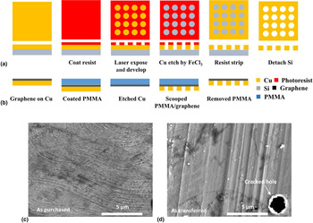
The preparation processes of suspended graphene membrane are presented in Fig. 1. There were two parts to prepare suspended graphene on Cu. The first part was the fabrication of a perforated Cu substrate by using the microfabrication technology illustrated in Fig. 1(a). The desired circular shape was patterned by a Maskless photolithography process after photoresist (AZ 1813, MicroChem.com) coated on Cu substrate. For the Maskless process, the laser writer (DWL 66-fs, Heidelberg Instruments) was used for an appropriate exposure followed by immersion in the developer. The resulting exposed patterns on Cu substrate were etched by FeCl3 (Iron trichloride) solution. Finally, the patterned Cu substrate was immersed in acetone to strip off the photoresist, rinsed in isopropyl alcohol and deionized (DI) water, and dried. The second part was the transferring graphene on the perforated Cu substrate shown in Fig. 1(b). Chemical Vapor Deposition (CVD) grown single graphene on Cu was purchased from Graphenea Inc. It was polycrystalline graphene which had ≤ 10 µm grain size (as purchased claimed by Graphenea). First, PMMA (Polymethyl methacrylate) was coated with graphene/Cu sample followed by etching Cu with FeCl3 solution. PMMA/graphene film was rinsed with DI water and scooped with the perforated Cu substrate. PMMA on top of graphene on Cu substrate was removed by acetone and rinsed with isopropyl alcohol and DI water.
Sample preparation and experimental set up. (a) Fabrication of a perforated Cu substrate, (b) transfer process of graphene on the Cu substrate, (c) before transferring graphene on Cu, (d) after transferring graphene on Cu.
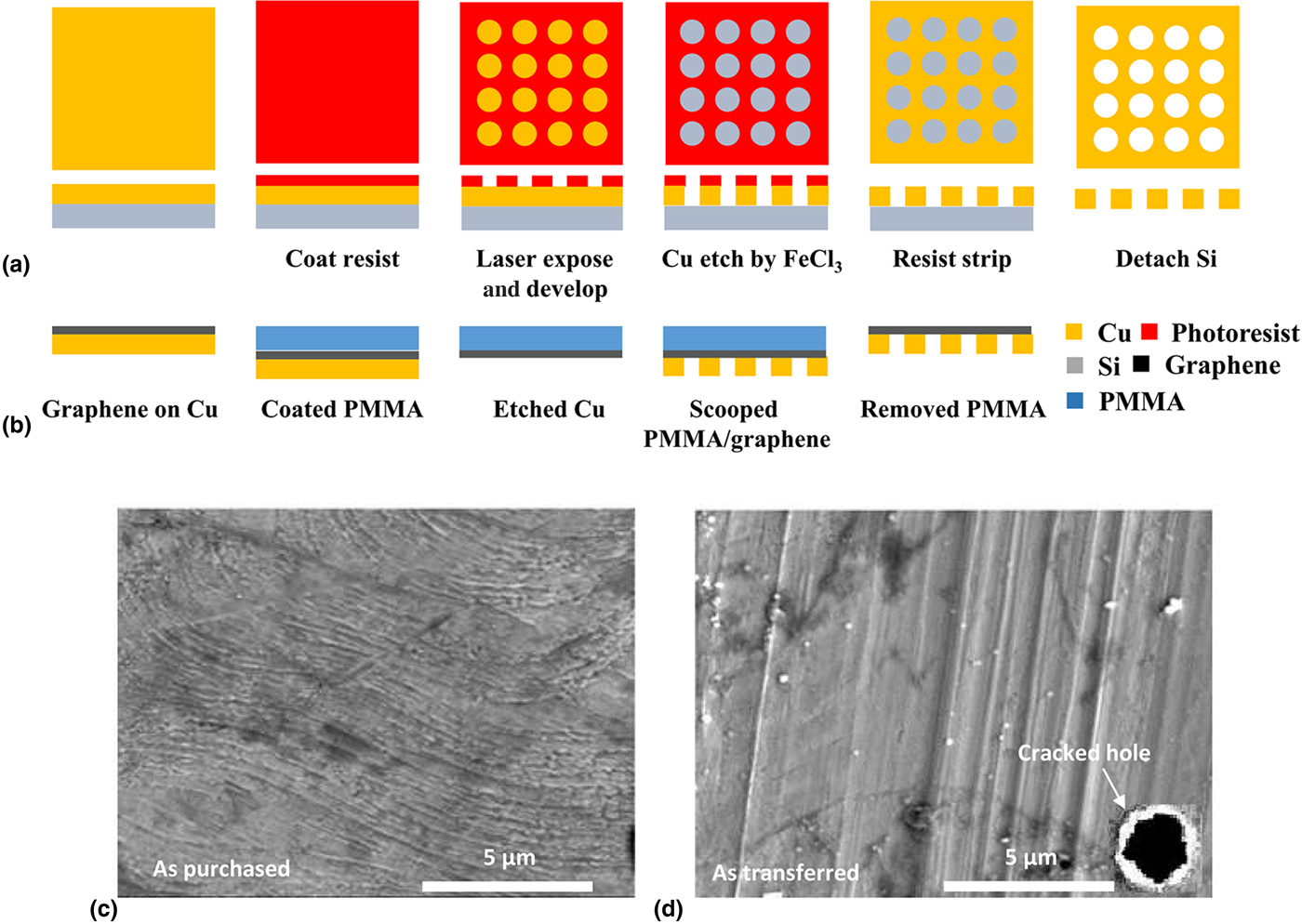
Figures 1(c)–1(d) show two SEM pictures before and after transfer of graphene. They do not clearly show the grain boundaries of graphene due to the presence of the copper substrate. On the contrary, transferred graphene suffers from severe cracking, which often happens during the transfer process. To ensure the quality of graphene in terms of crack, we have used, for measurements, only a successfully transferred sample without cracking on the suspended graphene; the inset of Figure 1(d) shows such cracking and we discarded the sample without further testing. This could be an indirect evidence that the quality in terms of cracking is managed over the transfer process.
Experimental setup and estimation of thermal properties
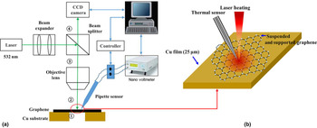
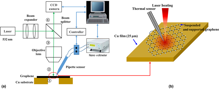
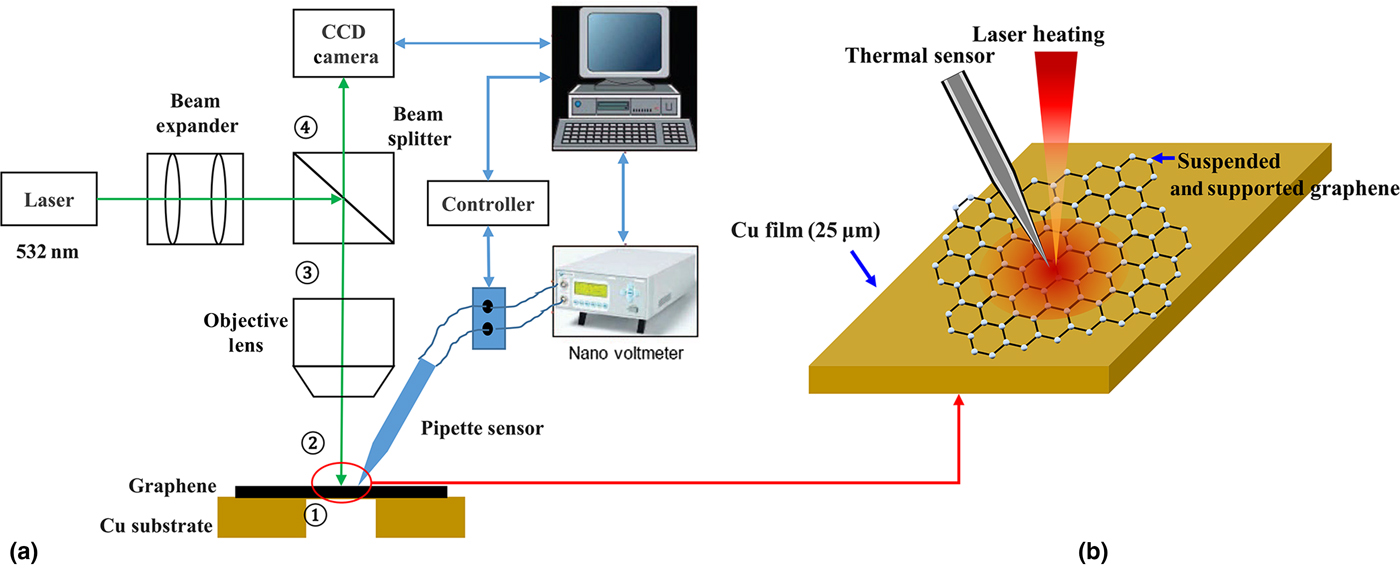
Figures 2(a)–2(b) show the experimental setup for measuring the temperature of graphene surfaces which were suspended and supported. The measurement setup consists of the optical system (long working distance lens, mirrors, and beamsplitter), the electric device (nanovoltmeter), a laser (532 nm, Opto Engin LLC), a charge-coupled device (CCD) camera (Mightex) and MTS. The laser is guided by the optical system on the sample surface to heat the sample. The CCD camera monitors the laser illumination and the landing of MTS on the sample in real time. Temperatures of suspended and supported graphene were measured by MTS which was fabricated by the thermocouple principle that can be found in our previously published articles.[Reference Shrestha, Lee, Chang, Kim, Rhee and Choi14, Reference Jeong, Lee, Shrestha, Horne, Das, Choi, Kim and Choi15] In every temperature measurement on the heated sample by using MTS, the consistent mechanical contact between MTS and the sample was ensured by the voltage measured by nanovoltmeter and CCD camera. In other words, the measured voltage by MTS significantly changes when MTS contacted with the heated sample. CCD camera simultaneously monitored the deformation of the sample surface while contacting with MTS. In addition, MTS was moved down vertically by 1μm by a motorized z-stage in every temperature measurement to obtain a good mechanical contact with the sample surface.
Experiment set-up. (a) Measurement set-up, (b) temperature measurement of suspended and supported graphene on Cu substrate.
Once the radial temperature profile is obtained on the surface of graphene (either suspended or Cu-supported), intrinsic (for suspended) and apparent (for Cu-supported) thermal conductivities can be estimated. The intrinsic thermal conductivity can be calculated by the Fourier's equation,
 $$Q = {\rm \;} \displaystyle{{2\pi kL\lpar {T_1-T_2} \rpar } \over {{\rm ln}(r_2/r_1)}},$$
where Q, k, L, T 1, T 2, r 1, and r 2 are the absorbed power, the thermal conductivity of suspended graphene, the thickness of suspended graphene, temperatures, radial positions from the center of the laser spot, respectively. The apparent thermal conductivity after the acquisition of surface temperature profile on a Cu-supported graphene will be linked with a COMSOL Multiphysics simulation (detailed in the section ‘Multiparameter fitting method with COMSOL Multiphysics and MATLB’) to estimate the ITR between graphene and Cu-substrate by using the multi-parameter fitting technique.[Reference Lagarias, Reeds, Wright and Wright16]
For the absorbed power which is needed to calculate thermal properties [i.e., Q in Eq. (2)], incident, reflected, and transmitted power were measured by a power meter (THORLABS PM100D) at different positions for the experiment. Transmitted power and incident power were measured at position (1) and (2) in Fig. 2(a), respectively. The power loss at the objective lens and reflected power were measured at position (3) and (4) in Fig. 2(a), respectively. With these measured powers, the absorbed power of the sample was calculated by Eq. (2)
 $$P_{{\rm absorbed}} = P_{{\rm incident}}-P_{{\rm reflected}}-P_{{\rm transmitted}}.$$
Considering various sources of uncertainties in this study, we have calculated the measurement uncertainty of thermal conductivity by the Root-Sum-Squared (RSS) method.[Reference Holman and Gajda17] It can be expressed by,
 $$u_k = \left[ {{\left( {\displaystyle{{\partial k} \over {\partial Q}}u_Q} \right)}^2 + {\left( {\displaystyle{{\partial k} \over {\partial R}}u_R} \right)}^2 + {\left( {\displaystyle{{\partial k} \over {\partial L}}u_L} \right)}^2 + {\left( {\displaystyle{{\partial k} \over {\partial \Delta T}}u_{\Delta T}} \right)}^2} \right]^{1/2},$$
where u k,, u Q, u R, u L, and u ΔT are the uncertainty of thermal conductivity, power measurement, radial position, thickness, and temperature measurement, respectively. The uncertainties of the power and the voltage were calculated by the standard deviations during measurement and the instrument specification. In addition, the uncertainties of temperature and radial position measurements were calculated by ΔT = ΔV/S and R = ln (r 2/r 1), where ΔT, ΔV, r, and S are temperature difference, voltage difference, radial position with a center at the laser focal spot and Seebeck coefficient, respectively.[Reference Shrestha, Lee, Chang, Kim, Rhee and Choi14]
Multiparameter fitting method with COMSOL Multiphysics and MATLB
To calculate the temperature profile of supported graphene on Cu heated by laser and, subsequently, compare it with experimentally measured one to estimate ITR, a COMSOL simulation software package was used to model the steady-state heat transfer in solid physics. The temperature profile obtained from simulation will be entered into an optimization routine with which the unknown parameter, ITR, will be estimated in an iterative way until the difference between experiment and simulation is minimized. This is one of inverse engineering problems.[Reference Moftakhari, Aghanajafi and Moftakhari Chaei Ghazvin18]. A schematic view of the graphene on Cu film for simulation is shown in Fig. S1. We have modeled ITR as a very thin layer of air present between graphene and Cu-substrate in the COMSOL simulation. The overall dimension of the graphene sample was 400 × 400 µm2. The thickness of graphene and Cu was 0.34 nm and 25 µm, respectively. Other thermophysical parameters of Cu and air were obtained from the COMSOL material library and the intrinsic thermal conductivity of graphene obtained from Eq. (1) was used for the simulation. The laser heat source was assumed to have the Gaussian intensity distribution and the point heat source was applied for the laser. The thermal conductivity of graphene was set in different values for in-plane and out of the plane because of its anisotropic nature. The difference between experimental and simulation data were numerically calculated and expressed in Eq. (4),
 $$f\,(x) = \mathop \sum \limits_{n = 1}^N \lpar {\emptyset_n^{{\rm sim}} -\emptyset_n^{{\rm exp}}} \rpar ^2$$
where f(x), x,  $\emptyset _n^{{\rm sim}} $ and
 $\emptyset _n^{{\rm exp}} $ are the difference function, parameters (a vector), simulation and experiment temperatures, respectively. In order for the multi-parameter fitting, the out-of-plane thermal conductivity of graphene, the absorbed power of the sample, and the air gap between graphene and copper were used for the input parameters. The multi-parameter fitting technique was used in MATLAB to find the optimizing parameters that fitted the experiment data with the simulation result.
Results & discussion
Figure S2 shows the result of MTS's calibration to find its Seebeck coefficient. The calibration of MTS was conducted in an insulated chamber filled with DI water from room temperature to 35°C. The Seebeck coefficient of MTS was determined by the slope in Fig. S2. This calculated Seebeck coefficient was used for determining temperature differences between two positions on the sample surface.
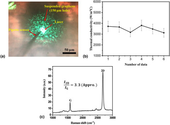
The temperature measurements on suspended graphene were conducted by MTS. Figure 3(a) presents the optical image of suspended graphene contacted to MTS. MTS contacted to suspended graphene and measured the voltage of the heated suspended graphene surface with different radial distances from the center of the laser spot. The distance between the center of the laser heating source and the MTS contact point was determined by counting the pixel of CCD image with a calibrated optical system. The measured voltage could be converted to its local surface temperature with the Seebeck coefficient of MTS and used for calculating thermal conductivity of suspended graphene in Fig. 3(b). Graphene was identified by optical Raman spectroscopy (Spectra-Physics, model 177G02) in Fig. 3(c). The ratio of the 2D band at ~2678/cm and G-band at ~1583/cm peak intensity in Fig. 3(c) presents a single layer of graphene, which means 2D peak is roughly 3.3 times more intense than the G peak.[Reference Ferrari, Meyer, Scardaci, Casiraghi, Lazzeri, Mauri, Piscanec, Jiang, Novoselov and Roth19]
Temperature measurement and Raman spectroscopy of suspended graphene. (a) Optical image of suspended graphene, (b) thermal conductivity of suspended graphene, (c) Raman spectrum of suspended graphene.
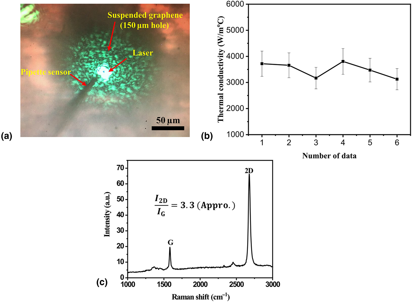
The thermal conductivity values for suspended graphene determined by Eq. (1) are ranged from 3126.4 to 3806.8 W/m°C as shown in Fig. 3(b). Eric Pop et al. investigated the effect of grain boundaries on thermal transport in graphene regarding ballistic thermal transport. From their results, single grain boundary across graphene nanoribbons (GNRs) decreased thermal conductance by 30~40% compared with a pristine GNRs.[Reference Serov, Ong and Pop20] Tej B. Limbu et al. also reported the grain size effect on thermal conductivity of polycrystalline graphene. They pointed out that there was degradation in thermal conductivity due to grain boundaries in polycrystalline graphene.[Reference Limbu, Hahn, Mendoza, Sahoo, Razink, Katiyar, Weiner and Morell21] Therefore, various reasons such as polycrystalline grain boundaries, point defects, and impurities like metal or polymer resulted from the fabrication processes can affect the thermal conductivity values of suspended graphene.[Reference Serov, Ong and Pop20–Reference Alemán, Regan, Aloni, Altoe, Alem, Girit, Geng, Maserati, Crommie and Wang24] For these reasons, a transferred CVD graphene sample can show different thermal conductivity values at different measured points. In addition, the thermal conductivity of suspended graphene differs due to the uncertainty as mentioned in Eq. (3). The uncertainties regarding the radial position, temperature difference, and the absorbed power resulted from the calibration of CCD image, pipette sensor, and instruments errors, and they were summarized in Table I. The overall uncertainty in the measurement of thermal conductivity of suspended graphene was calculated to be 13.2% and the mean thermal conductivity is estimated at 3492 ± 461 W/m°C.
Summarized uncertainties in experimental measurement.

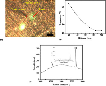
Figure 4 presents the temperature measurements of supported graphene on Cu. The temperature measurement of supported graphene was conducted the same way with that of measuring suspended graphene sample. The voltages were measured by MTS with different radial distances from the center of the laser in Fig. 4(a) and they were converted to temperatures in Fig. 4(b). The absorbed power of the sample could not be measured because the reflected laser was scattered by the rough surface of the copper substrate. Therefore, the absorbed power on the supported graphene on Cu was set as one of the unknown parameters for the multi-parameter fitting. This measured temperature of supported graphene on Cu by MTS was used for multiple parameter fitting to compare with the simulated temperature profile. In addition, single graphene on Cu was identified by optical Raman spectroscopy in Fig. 4(c).
Temperature measurement and Raman spectroscopy of supported graphene on Cu. (a) Optical image of supported graphene on Cu, (b) temperature measurement result. (c) Raman spectrum.
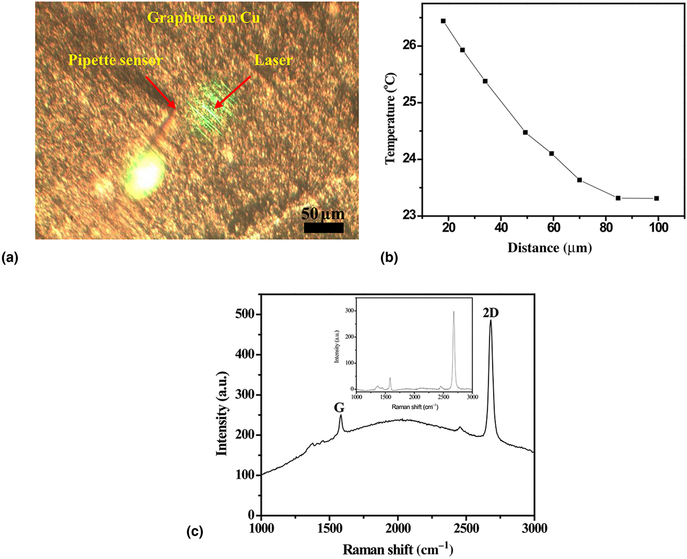
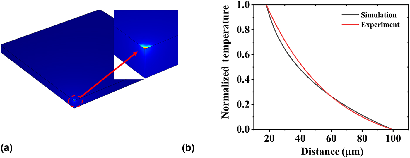
Figure 5 exhibits temperature distribution of the surface of supported graphene on Cu and the fitted simulation data with experiment result. To determine the optimizing parameters for estimating interface thermal resistance between graphene and Cu substrate, interface distance, out of plane thermal conductivity and absorbed power was used for input parameters.
Fitted simulation data with experiment result. (a) Temperature distribution of the surface of graphene/air/Cu, (b) fitting result with optimized data.
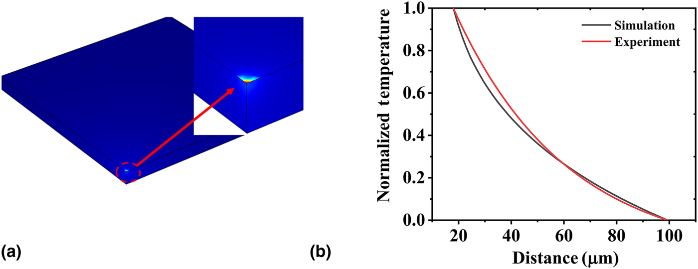
The best-fit parameters of the interface distance, out-of-plane thermal conductivity, and absorbed power were determined by multiple parameters fitting and they are summarized in Table II. These optimized parameters were used for estimating ITR between graphene and Cu. The estimated interface thermal resistance was 2.3 × 10⁻⁷ m2 °C/W. In Fig. 5(b), the red line and black line denote the experimental data and the numerical prediction result with the best-fit parameters, respectively. The average difference between the experiment and simulation result after the optimization routine was estimated to be 6.9%. This difference resulted from experimental measurement uncertainties related to temperature measurement, the thermal resistance between MTS and surface of the sample, and sample condition having impurities, structure defects, and a polycrystalline structure.
Best fit parameters in multiple parameter fitting analysis.

Conclusions
In summary, the interface thermal resistance between graphene and Cu substrate have been studied by using the multi-parameter fitting method linked with surface temperature measurement by the micropipette thermography technique. In the experimental works, the temperature of suspended single graphene and temperature of supported graphene were measured by a micropipette thermal sensor at room temperature. With the measured temperature profile on suspended graphene, one can estimate the thermal conductivity of suspended graphene at 3492 ± 453 W/m°C. The multi-parameter fitting method reveals the best-fitted value of interface distance to be 5.92 nm. In turn, the interface thermal resistance was estimated at 2.3 × 10⁻⁷ m2 °C/W. The average difference between experiment and simulation result during multi-parameter fitting was 6.9%. This difference was related to the uncertainties of experimental measurements such as temperature measurement, radial position, and power measurement.
Supplementary material
The supplementary material for this article can be found at https://doi.org/10.1557/mrc.2018.219