
1. Introduction and background
Taylor–Couette flow (TCF) occurs in the gap between two concentric cylinders with one or both rotating. It has been of sustained interest to the fluid mechanics community, rheologists, process engineers and mathematicians over the past century (Taylor Reference Taylor1923). Despite its simple geometrical configuration, TCF of Newtonian fluids displays a vast array of complex dynamics. This includes a wide variety of steady, unsteady, chaotic or turbulent flow states (Coles Reference Coles1965; Andereck, Liu & Swinney Reference Andereck, Liu and Swinney1986; Akonur & Lueptow Reference Akonur and Lueptow2003; Dutcher & Muller Reference Dutcher and Muller2009; Grossmann, Lohse & Sun Reference Grossmann, Lohse and Sun2016; Gul, Elsinga & Westerweel Reference Gul, Elsinga and Westerweel2018), occurring when either one or two cylinders rotate, in contra-rotation or corotation. In the most common case in which only the inner cylinder rotates and the outer cylinder is fixed, the flow can be characterised using a single Reynolds number,
 \begin{equation} Re=\rho\varOmega r_id/\mu,\end{equation}
where  $\rho$ is the fluid density,
 $\mu$ the dynamic viscosity,
 $\varOmega$ the inner cylinder rotation speed and
 $d=r_o-r_i$ the gap width, i.e. the difference between the inner and outer cylinder radii,
 $r_i$ and
 $r_o$, respectively. The system geometry can be characterised using two non-dimensional parameters: the radius ratio
 $\eta =r_i/r_o$; and the aspect ratio
 ${AR}=L/d$, where L is the cylinder length. The first parameter describes the gap width and streamline curvature in a simple shear flow, both having an influence on the stability threshold for Newtonian (Taylor Reference Taylor1923) but also non-Newtonian fluids (Larson, Shaqfeh & Muller Reference Larson, Shaqfeh and Muller1990; Pakdel & McKinley Reference Pakdel and McKinley1996).
At low  $Re$ in Newtonian fluids, a purely azimuthal and uniform shear flow exists in the gap, known as the circular Couette flow (CF). This flow becomes unstable once a critical
 $Re$ is reached, and a series of toroidal counter-rotating vortices form in the annulus: this is known as the Taylor vortex flow (TVF). The number of counter-rotating vortices along the gap corresponds to the spatial wavelength of the instability,
 $\lambda$. A further increase in
 $Re$ causes this state to become unstable and undergo sinusoidal axial oscillations (wavy Taylor vortex flow (WTVF)), making it non-axisymmetric. Additional frequencies appear as
 $Re$ is further increased, leading to a more complex wavy flow (Coughlin & Marcus Reference Coughlin and Marcus1992a,Reference Coughlin and Marcusb) which ultimately becomes turbulent (Grossmann et al. Reference Grossmann, Lohse and Sun2016).
Because of this rich set of dynamic states in simple fluids, TCF has been widely used as a means to study flow transitions and instabilities in more complex systems, such as non-Newtonian fluids (Fardin, Perge & Taberlet Reference Fardin, Perge and Taberlet2014), frequently encountered in industrial applications (Chhabra & Richardson Reference Chhabra and Richardson1999). Polymer solutions (Larson & Desai Reference Larson and Desai2015) or worm-like micellar solutions (WMS) (Divoux et al. Reference Divoux, Fardin, Manneville and Lerouge2016) are useful model fluids to describe the behaviour of such systems. The latter have received increased attention in recent years (Fardin et al. Reference Fardin, Lopez, Croso, Grégoire, Cardoso, McKinley and Lerouge2010, Reference Fardin, Ober, Grenard, Divoux, Manneville, McKinley and Lerouge2012; Perge, Fardin & Manneville Reference Perge, Fardin and Manneville2014; Mohammadigoushki & Muller Reference Mohammadigoushki and Muller2017; Haward, Hopkins & Shen Reference Haward, Hopkins and Shen2020; Hopkins, Haward & Shen Reference Hopkins, Haward and Shen2020) while the former have been extensively used in the literature for several decades (see the remainder of § 1), and will also be employed in this study. Two of their most common non-Newtonian properties are shear-thinning and viscoelasticity. The former leads to a dynamic viscosity  $\mu$ that depends on the shear rate
 $\dot {\gamma }$ (e.g. in a power law fashion,
 $\mu \sim \dot {\gamma }^{n-1}$ with
 $n$ the flow index). Elasticity confers a ‘solid-like’ behaviour to the fluid, with a complex shear modulus
 $G^*$ that comprises an elastic part
 $G'$ and a viscous part
 $G"$ such as
 $G^*=G'+iG"$. This property is characterised by the existence of an elastic/relaxation time scale of the fluid,
 $t_e$. Such properties are influenced by many factors including the molecular weight, polymer concentration, conformation of the polymer chains and entanglement (Larson & Desai Reference Larson and Desai2015). By using low concentrations of high molecular weight linear polymers in a sufficiently viscous solvent, one may produce ‘Boger’ fluids (Boger Reference Boger1977; James Reference James2009), i.e. elastic fluids for which the polymer contribution to the viscosity is small compared with the solvent viscosity, and for which the apparent viscosity is thus constant (Newtonian). Equally, by selecting different polymers and solvent viscosities, one can vary elasticity and shear-thinning almost independently, exploring the relative influence of these parameters on TCF over a broad parameter space.
1.1. Elastic and elasto-inertial TCFs
The degree to which a fluid has an elastic response to the flow is expressed by the Weissenberg number,  ${Wi}$. In a Taylor–Couette system, this number can be defined as
 ${Wi}=t_e/\dot {\gamma }$, where
 $\dot {\gamma }=\varOmega r_i/d$ is the nominal shear rate in the gap. The competition between elastic and viscous effects is then expressed by the elastic number,
 \begin{equation} {El}=\frac{{Wi}}{Re}=\frac{t_e}{t_v}=\frac{t_e\mu}{\rho d^2},\end{equation}
where  $t_v=\rho d^2/\mu$ is the viscous time scale. Here
 ${El}$ only depends on the fluid and geometric properties. Based on its value, the fluid can be classified as weakly elastic (
 ${El} < 10^{-2}$), moderately elastic (
 $10^{-2} < {El} < 1$) or highly elastic (
 ${El}>1$) (Dutcher & Muller Reference Dutcher and Muller2011, Reference Dutcher and Muller2013; Latrache et al. Reference Latrache, Abcha, Crumeyrolle and Mutabazi2016). In the range of low elasticity (i.e.
 ${El}\ll 1$) and with increasing
 $Re$, transitions similar to Newtonian fluids have been recovered (Crumeyrolle, Mutabazi & Grisel Reference Crumeyrolle, Mutabazi and Grisel2002; Dutcher & Muller Reference Dutcher and Muller2011).
At vanishing  $Re$ but moderate or high
 ${El}$, a purely elastic CF–TVF transition exists (Larson et al. Reference Larson, Shaqfeh and Muller1990), and flows may even exhibit a chaotic behaviour (Groisman & Steinberg Reference Groisman and Steinberg2004; Fardin et al. Reference Fardin, Lopez, Croso, Grégoire, Cardoso, McKinley and Lerouge2010, Reference Fardin, Ober, Grenard, Divoux, Manneville, McKinley and Lerouge2012; Mohammadigoushki & Muller Reference Mohammadigoushki and Muller2017), which is called elastic ‘turbulence’, despite the relative absence of inertia (Larson Reference Larson2000), as it shows chaotic and disordered features usually attributed to turbulence (Groisman & Steinberg Reference Groisman and Steinberg2000; Steinberg Reference Steinberg2019; Varshney & Steinberg Reference Varshney and Steinberg2019).
At both non-negligible  $Re$ and
 ${El}$ values, elasto-inertial instabilities (primary or secondary) occur (Steinberg & Groisman Reference Steinberg and Groisman1998). They involve non-axisymmetric flow states and standing or travelling elastic waves such as ribbons (RIB) (Baumert & Muller Reference Baumert and Muller1999; Latrache et al. Reference Latrache, Abcha, Crumeyrolle and Mutabazi2016), spiral vortex flow (SVF) (Avgousti & Beris Reference Avgousti and Beris1993; Mohammadigoushki & Muller Reference Mohammadigoushki and Muller2017) and rotating spiral waves (RSW) (Groisman & Steinberg Reference Groisman and Steinberg1996; Thomas, Sureshkumar & Khomami Reference Thomas, Sureshkumar and Khomami2006; Dutcher & Muller Reference Dutcher and Muller2013; Lacassagne et al. Reference Lacassagne, Cagney, Gillissen and Balabani2020). Upon increasing
 $Re$ or
 ${El}$, such prechaotic states are replaced by unsteady, chaotic flow states, that have been called disordered oscillations (DO) (Groisman & Steinberg Reference Groisman and Steinberg1996), defect mediated turbulence (DMT) or spatio–temporal intermittency (STI) (Latrache, Crumeyrolle & Mutabazi Reference Latrache, Crumeyrolle and Mutabazi2012; Latrache et al. Reference Latrache, Abcha, Crumeyrolle and Mutabazi2016). They all consist in a gradual transition to elasto-inertial turbulence (EIT) (Dutcher & Muller Reference Dutcher and Muller2013; Liu & Khomami Reference Liu and Khomami2013; Perge et al. Reference Perge, Fardin and Manneville2014; Lacassagne et al. Reference Lacassagne, Cagney, Gillissen and Balabani2020). Elasto-inertial (and elastic) turbulence induces spatial and temporal chaos in fluids that would otherwise have been flowing in laminar states without elasticity, promoting mixing and momentum transfer (Groisman & Steinberg Reference Groisman and Steinberg2004).
1.2. Shear-thinning TCFs with negligible elasticity
In shear-thinning fluids with negligible elasticity, the typical transition pattern is ‘Newtonian-like’: CF–TVF–WTVF (Escudier, Gouldson & Jones Reference Escudier, Gouldson and Jones1995; Bahrani et al. Reference Bahrani, Nouar, Neveu and Becker2015; Cagney & Balabani Reference Cagney and Balabani2019b; Topayev et al. Reference Topayev, Nouar, Bernardin, Neveu and Bahrani2019). In the small gap limit, a decrease in the critical Reynolds number for the formation of Taylor vortices  $Re_c^{TVF}$ (destabilisation) occurs with increased shear-thinning. This has been observed both experimentally (Escudier et al. Reference Escudier, Gouldson and Jones1995; Cagney & Balabani Reference Cagney and Balabani2019a; Cagney, Lacassagne & Balabani Reference Cagney, Lacassagne and Balabani2020) and numerically (Ashrafi & Khayat Reference Ashrafi and Khayat2000; Caton Reference Caton2006). In the large gap limit, shear-thinning has a non-monotonic effect on
 $Re_c^{TVF}$, (Sinevic, Kuboi & Nienow Reference Sinevic, Kuboi and Nienow1986; Lockett, Richardson & Worraker Reference Lockett, Richardson and Worraker1992; Alibenyahia et al. Reference Alibenyahia, Lemaitre, Nouar and Ait-Messaoudene2012; Cagney & Balabani Reference Cagney and Balabani2019a).
The spatial wavelength of the TVF has been found to increase with increased shear-thinning, as observed in experiments and the linear stability analysis by Bahrani et al. (Reference Bahrani, Nouar, Neveu and Becker2015) (in a large gap flow cell), laser Doppler velocimetry measurements by Escudier et al. (Reference Escudier, Gouldson and Jones1995) or particle image velocimetry (known as PIV) in Cagney & Balabani (Reference Cagney and Balabani2019b). From the two later works and numerical simulations by Topayev et al. (Reference Topayev, Nouar, Bernardin, Neveu and Bahrani2019) and Alibenyahia et al. (Reference Alibenyahia, Lemaitre, Nouar and Ait-Messaoudene2012), shear-thinning was found to modify the structure of the Taylor vortices, by making individual vortices asymmetric, and increasing the amplitudes of the travelling waves at the inward and outward jets. Sparse data on the critical  $Re$ value for the TVF to WTVF (Bahrani et al. Reference Bahrani, Nouar, Neveu and Becker2015; Cagney et al. Reference Cagney, Lacassagne and Balabani2020) suggest that the TVF to WTVF transition happens at lower
 $Re$ values with increased shear-thinning. Shear-thinning also alters the structure of the wavy vortices (Cagney & Balabani Reference Cagney and Balabani2019b; Cagney et al. Reference Cagney, Lacassagne and Balabani2020).
1.3. Combined shear-thinning and elasticity
The effects of shear-thinning and elasticity have been studied separately in the literature, with elastic fluids having received more attention to date. There is still a lack of experimental work on fluids combining the two properties. In studies focused on elastic fluids, shear-thinning, when reported, is generally mild and typically neglected. However, even moderate shear-thinning can have a significant impact on the base flow structure, and thus on the development of elastic instabilities. The onset of the primary instability is found at lower critical  $Re$ values than in Newtonian fluids, regardless of shear-thinning (Larson, Muller & Shaqfeh Reference Larson, Muller and Shaqfeh1994; Crumeyrolle et al. Reference Crumeyrolle, Mutabazi and Grisel2002; Dutcher & Muller Reference Dutcher and Muller2011, Reference Dutcher and Muller2013; Schaefer, Morozov & Wagner Reference Schaefer, Morozov and Wagner2018; Cagney & Balabani Reference Cagney and Balabani2019b; Cagney et al. Reference Cagney, Lacassagne and Balabani2020). The main challenge resides in describing higher-order, higher-
 $Re$ flow transitions.
Latrache and coworkers performed a series of experimental works using shear-thinning and viscoelastic polyethylene oxide (PEO) solutions in low-viscosity solvents. They reported several types of transition patterns, from Newtonian-like (Crumeyrolle et al. Reference Crumeyrolle, Mutabazi and Grisel2002) at  ${El}<0.03$, to ‘elastic-like’ with RIB (Crumeyrolle et al. Reference Crumeyrolle, Mutabazi and Grisel2002, Reference Crumeyrolle, Latrache, Mutabazi and Ezersky2005) and EIT states (Latrache et al. Reference Latrache, Crumeyrolle and Mutabazi2012, Reference Latrache, Abcha, Crumeyrolle and Mutabazi2016; Abcha et al. Reference Abcha, Kelai, Latrache, Crumeyrolle and Mutabazi2018). In Crumeyrolle et al. (Reference Crumeyrolle, Latrache, Mutabazi and Ezersky2005) and Latrache et al. (Reference Latrache, Abcha, Crumeyrolle and Mutabazi2016), DMT was reported, entailing a local collision of RIB waves leading to a spatio–temporal heterogeneity of the RIB map. The multiplication of such features ultimately leads to a fully disordered flow that can be labelled DO or EIT. In a recent work (Lacassagne et al. Reference Lacassagne, Cagney, Gillissen and Balabani2020), we reported a similar behaviour of elasticity promoting local anomalies in the flow, this time in a non-shear-thinning Boger fluid. The mechanism was yet different from DMT, as it consisted in merging and splitting of base Taylor vortices crossed by axial RSW waves, instead of defects in RIB amplitude. It thus appears that the mechanisms for transition to EIT are greatly affected by the shear-thinning behaviour of the fluid. Dutcher & Muller (Reference Dutcher and Muller2009), Dutcher & Muller (Reference Dutcher and Muller2011) and Dutcher & Muller (Reference Dutcher and Muller2013) also used shear-thinning and elastic PEO solutions to study the effects of weak and intermediate elasticity. Comparing their results with those of Crumeyrolle et al. (Reference Crumeyrolle, Mutabazi and Grisel2002), the authors argued that the difference in the ratio of polymer-to-solvent viscosity may explain the different flow transitions observed at similar
 ${El}$ values. This polymer-to-solvent viscosity ratio is intrinsically related to the shear-thinning property: the higher this ratio, the more the polymer contributes to the overall viscosity and the stronger the shear-thinning level is likely to become.
In our recent work (Cagney et al. Reference Cagney, Lacassagne and Balabani2020), xanthan gum (XG) solutions with systematically increasing concentration were produced, yielding fluids with both increasing shear-thinning and elastic properties. Even at high- ${El}$ values, the Newtonian-like transition pattern associated with shear-thinning fluids was retrieved, and no typical features of elastic behaviours (RSW, RIB, EIT) were reported. In this study, as in those of Latrache and coworkers, disentangling the effects of shear-thinning and elasticity was difficult, as both properties were varied simultaneously with the polymer concentration. Moreover, many previous studies examining TCF of XG solutions did not fully characterise the rheology and assumed negligible elasticity, making it challenging to distinguish the effects of either phenomenon on the flow (Bahrani et al. Reference Bahrani, Nouar, Neveu and Becker2015; Masuda et al. Reference Masuda, Horie, Hubacz, Ohta and Ohmura2017; Elçiçek & Güzel Reference Elçiçek and Güzel2020a,Reference Elçiçek and Güzelb).
Finally, in TCFs of shear-thinning and elastic WMS, travelling vortices (SVF), standing waves (RIB) and transition to EIT have been reported. In Perge et al. (Reference Perge, Fardin and Manneville2014) the typical transition pattern is CF–RIB–EIT in a significantly shear-thinning fluid ( $n=0.45$) at
 ${El}\sim 1$. In Mohammadigoushki & Muller (Reference Mohammadigoushki and Muller2017), travelling vortices that could be SVF were reported, as well as a transition to EIT.
Experimental data on TCF of fluids that are both shear-thinning and viscoelastic are inconclusive regarding how shear-thinning affects elastic instabilities and transitions. It appears that elastic fluids may exhibit a Newtonian-like transition pattern, in the low-elasticity limit (Crumeyrolle et al. Reference Crumeyrolle, Mutabazi and Grisel2002; Dutcher & Muller Reference Dutcher and Muller2011), but also at high  ${El}$ when they are also shear-thinning (Cagney et al. Reference Cagney, Lacassagne and Balabani2020), suggesting that shear-thinning may act to reduce or suppress elastic instabilities. Such a shear-thinning modification of elastic effects has also been observed in other types of flows (PEO in serpentine microchannel (Casanellas et al. Reference Casanellas, Alves, Poole, Lerouge and Lindner2016), WMS flow past micropins (Haward et al. Reference Haward, Hopkins and Shen2020)). On the other hand, shear-thinning is known to be conditional for some elastic instabilities to develop, for example in viscoelastic (pressure driven) channel flows (Bodiguel et al. Reference Bodiguel, Beaumont, Machado, Martinie, Kellay and Colin2015; Barlow et al. Reference Barlow, Hemingway, Clarke and Fielding2019).
In this work, we thus aim at disentangling the effects of shear-thinning and elasticity on TCF transitions and patterns in polymer solutions. We present flow visualisation measurements of TCF for polymer solutions with variable degrees of elasticity and shear-thinning. The remainder of the paper is structured as follows. Firstly, the experimental system is described in § 2. The results of flow visualisation experiments are then reported in § 3. In § 4, the combined effects of shear-thinning and elasticity on transitions to TVF and WTVF and EIT, including potential suppression of the latter, are discussed, and some concluding remarks can be found in § 5.
2. Experiments
2.1. Taylor–Couette cell
The experiments were performed in a custom made TCF cell. It comprised an outer cylinder made of an acrylic pipe, mounted vertically between two acrylic plates, and a black polytetrafluoroethylene (known as PTFE) inner cylinder. The latter had a conical tip complementary to a dent in a bottom plate which allowed reduction of bottom friction while, together with a ball bearing at the top lid, ensuring alignment between the inner and outer cylinder. The top and bottom lids were stationary, with a  $\sim 3$ mm gap between lid and cylinder at both ends. The cylinder was driven from the top using a stepper motor (SmartDrive Ltd, Cambridge, UK), the rotation of which could be controlled to a high degree of precision by a 52 000 microstep/revolution controller (SmartDrive Ltd, Cambridge, UK). The inner chamber, which was completely filled with working fluid, had an axial length of
 $L = 135$ mm. The inner and outer radii of the flow cell were 21.66 mm and 27.92 mm, respectively. The radius ratio was thus
 $\eta = 0.77$, the gap width was
 $d=6.26$ mm and the aspect ratio was
 ${AR}=21.56$. The geometric parameters are sketched on figure 1. The flow section was enclosed in a rectangular chamber in which water was recirculated via a temperature bath to ensure that the temperature remained constant and close to 20
 $\,^{\circ }\mathrm {C}$ throughout the experiments. The temperature within the flow cell was measured immediately before and after each experiment, and it was found to vary by less than 0.2
 $\,^{\circ }\mathrm {C}$.
Sketch of the test section and flow visualisation system.

2.2. Polymer solutions and rheological characterisation
Optically clear shear-thinning and viscoelastic polymer solutions were prepared by dissolving XG (Sigma Aldrich) into a mixture of glycerol and deionized water. The weight-averaged molecular mass  $M_w$ was measured by size exclusion chromatography and found to be equal to
 $1.76\times 10^6\ \mathrm {g~mol}^{-1}$ (Cagney et al. Reference Cagney, Lacassagne and Balabani2020).
Various degrees of elasticity and shear-thinning of the XG solutions were achieved by varying solution composition (polymer concentration and glycerol volume fractions). For comparison, a Boger fluid was prepared by dissolving small concentrations of PAAM ( $M_w=5.5\times 10^6\ \mathrm {g~mol}^{-1}$, Sigma Aldrich) into deionized water–glycerol mixtures. Polymers were progressively added to the solvent and left to dissolve overnight without any agitation, to prevent polymer chain destruction in the preparation process, and the mixture was finally homogenised by gentle shaking. Polymer type, concentration and solvent composition and viscosity for each working fluid used in this work are listed in table 1. The sample naming convention used throughout the paper is the following: letters correspond to the polymer used (XG for xanthan gum, P for PAAM, N for none), the last two digits after the ‘
 $-$’ sign to the glycerol volume fraction (e.g.
 $-$72 for
 $72\,\%$) and the middle number, if present, to the polymer concentration in parts per million in weight (ppm).
Polymer solutions and their rheological properties at  $20\,^{\circ }\textrm {C}$. The sample labelling scheme is the following (ID column): XXiii-jj where XX is the polymer molecule used (N if no polymer); iii is the polymer concentration in ppm (empty if no polymer); and jj is the glycerol volume fraction in the solvent in volume
 $\%$.

The steady-shear rheology of all working fluids was measured using a rotational rheometer (ARES, TA Instruments) equipped with a Couette geometry (inner radius 32 mm, outer radius 34 mm) in steady-shear mode. All XG samples exhibit shear-thinning. The shear viscosity of the PAAM sample remains almost constant for a wide range of shear rates. Flow curves (viscosity versus shear rate) for all working fluids are shown in figure 2. The shear-thinning data can be described using a Carreau model,
 \begin{equation} \mu(\dot{\gamma})=\mu_{\infty}+(\mu_0-\mu_{\infty})(1+(t_c\dot{\gamma} )^2)^{(n_c-1)/2}, \end{equation}
where  $\mu _{\infty }$ and
 $\mu _0$ are viscosity plateau values at infinite and zero shear, respectively,
 $t_c$ is the characteristic Carreau time scale and
 $n_c$ is the Carreau flow index. The fitted expressions are plotted on figure 2 as full lines. The estimated parameters for each fluid are also displayed in table 1. The ratio
 $\mu _0/\mu _{\infty }$ (reported in the last column of table 1) indicates the difference between so-called Boger fluids, for which the viscosity can be assumed constant with
 $\mu _0/\mu _{\infty }\sim 1$, and shear-thinning fluids for which
 $\mu _0/\mu _{\infty } \gg 1$. For a given fluid, the degree of shear-thinning (slope of the curve) was shear-rate dependent. This means that the effective shear-thinning behaviour varied as the rotation speed was varied. It is thus convenient to define a shear-rate dependent, ‘effective’ flow index from the local slope of the flow curve in a log–log space (sketched on figure 2, see Coronado-Matutti, Souza Mendes & Carvalho (Reference Coronado-Matutti, Souza Mendes and Carvalho2004), Cagney & Balabani (Reference Cagney and Balabani2019b) and Cagney et al. (Reference Cagney, Lacassagne and Balabani2020)),
 \begin{equation} n_e=\frac{\partial \log (\mu)}{\partial \log (\dot{\gamma})}+1, \end{equation}
where  $n_e$ is equivalent to the previously defined flow index
 $n$, but accounts for the non-power-law behaviour via shear-rate dependency. An effective flow index close to unity means that the fluid behaves as a Newtonian fluid, and the effective flow index decreases with increasing shear-thinning behaviour. While
 $n_c$ may vary non-monotonically with polymer concentration,
 $n_e$ always decreases with increasing polymer concentration at a given shear rate and for a given solvent, and is a better indication of the degree of shear-thinning in each fluid (Cagney et al. Reference Cagney, Lacassagne and Balabani2020).
Viscosity as a function of shear rate for polymer solutions (filled symbols for XG; open symbols for polyacrylamide (PAAM)) at various concentrations and in solvents of three different glycerol volume fractions:  $25\,\%$ (triangles);
 $50\,\%$ (circles); and
 $72\,\%$ (squares). Expected solvent constant viscosities
 $\mu _s$ are derived from Volk & Kähler (Reference Volk and Kähler2018) and plotted as dotted lines. The measured viscosity for the reference Newtonian case (
 $72\,\%$ glycerol in water) is represented by black crosses.

The elastic properties of the samples were quantified by oscillatory shear experiments on the same rheometer and geometry. The evolution of  $G'$ and
 $G"$ with oscillation frequency were measured for
 $\gamma =5\,\%$. The
 $G'$ and
 $G"$ frequency sweeps are shown in figure 3.
Here  $G'$ (open symbols) and
 $G''$ (filled symbols) moduli for XG and PAAM solutions at various concentrations and in various glycerol water solvents.

For this study, a common way to estimate elastic time scales for the various types of fluids used and compare them, regardless of the solvent contribution to viscosity, was needed. To do so, the loss modulus curves from figure 3 were corrected by removing the contribution of the solvent viscosity (Zirnsak, Boger & Tirtaatmadja Reference Zirnsak, Boger and Tirtaatmadja1999), such that
 \begin{equation} \widetilde{G"}=G"-\mu_s \omega. \end{equation}
The elastic time scale could then be obtained from the crossover frequency  $\widetilde {\omega _c}$ between G′ and
 $\widetilde {G"}$ curves (not shown in figure 3 for the sake of readability), such that
 $t_e=2 {\rm \pi}/\widetilde {\omega _c}$. Doing so, one could access the polymer time scale regardless of the solvent used (even in fluids for which the solvent contribution to the overall viscosity is large compared with the polymer one, and for which no crossover between G′ and
 $G"$ can be observed in figure 3). Estimated time scales agreed with those estimated from Zimm approximation or multimode Maxwell fitting on G′ and
 $G"$ curves (Öztekin, Brown & McKinley Reference Öztekin, Brown and McKinley1994).
2.3. Flow visualisation experiments
The flow was visualised by adding reflective mica flakes to the fluid (Cornelissen  $\&$ Son, Pearl Lustre Pigments), at a volume fraction of the order of
 $10^{-4}$, similar to previous studies (Cagney & Balabani Reference Cagney and Balabani2019b; Cagney et al. Reference Cagney, Lacassagne and Balabani2020). Images of a vertical strip along the cylinder's axial dimension were acquired by a Phantom Miro 340 camera (see figure 1). The frame rate
 $f_s$ was adjusted throughout the experiments in order to achieve high temporal resolution of the Reynolds number range studied. For ramp-up and steady-state experiments, the frame rates used allowed all temporal frequencies in the flow to be resolved.
The  $2176\times 16$ pixel images were horizontally averaged to form an axial intensity profile for each instance. All such profiles were compiled into a matrix, or flow map, showing the evolution of the intensity profile over time or any time dependent parameter, such as
 $Re$. In a second step, the flow maps were divided into segments of
 $N_c=256$ columns (successive snapshots), with a 50
 $\%$ overlap, in order to calculate the average fast Fourier transform (FFT) for each row (i.e. each axial location) in each segment. All the averaged spectra were subsequently compiled to form a frequency map (Cagney & Balabani Reference Cagney and Balabani2019b). This map shows the evolution of the temporal frequencies of the flow as a function of time or
 $Re$. On frequency maps, a clear ridge may appear for regions with
 $f=f_\varOmega /2{\rm \pi}$, with fainter additional ridges at
 $f=k\times f_\varOmega /2{\rm \pi}$. These ridges arise from the ability of the visualisation method to detect the rigid body rotation frequency of the inner cylinder and its harmonics, and should not be interpreted as fluid flow frequencies.
In this work, the focus is on ramp-up experiments:  $\varOmega$ was increased at a constant rate,
 $\mathrm {d}\varOmega /\mathrm {d}t$, up to a maximum rotation speed
 $\varOmega _{max}$, which led to an increase in the Reynolds number up to
 $Re_{max}\simeq 300$. For shear-thinning fluids,
 $Re$ was computed using an effective viscosity
 $\mu (\dot {\gamma })$ derived from Carreau fittings, and thus increases nonlinearly with
 $\varOmega$. The flow maps resolution in terms of Reynolds number is quantified by the ratio
 $1/{\rm \Delta} Re$, reported in table 2, where
 ${\rm \Delta} Re$ is the average Reynolds number variation between two successive images. The (Newtonian) non-dimensional acceleration rate is defined as
 \begin{equation} \varGamma_0=\frac{\mathrm{d}Re}{\mathrm{d}t^*}=\frac{\rho^2 r_i d^3}{\mu^2}\frac{\mathrm{d}\varOmega}{\mathrm{d}t},\end{equation}
where  $t^*=t/t_v$ is the time divided by the viscous time scale. This acceleration rate must be kept low (typically
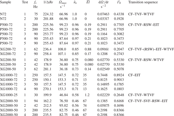
 $\varGamma _0 < 1$) to ensure that flow states are independent of the cylinder acceleration, i.e. that the ramp-up can be treated as a quasi-static process (Dutcher & Muller Reference Dutcher and Muller2009). In the Appendix of the present work, we present an investigation of the effects of acceleration on our experimental conditions, achieved by performing specific experiments in which the acceleration rate was varied over three decades. Based on the results of this investigation, the acceleration rates used for the main set of experiments (§ 3) were selected. Values of ramp-up parameters are reported in table 2. Values of the Nahme–Griffith number (see definition in supplementary data, available at https://doi.org/10.1017/jfm.2021.104) were estimated to be of order
 $10^{-1}$ at most for all working fluids at all shear rates, thus indicating that viscous heating effects are negligible (White & Muller Reference White and Muller2002a,Reference White and Mullerb).
Experimental conditions for ramp-up experiments, and transition sequence reported. The samples rheological characterisation is reported in table 1.

For shear-thinning fluids,  ${El}$ and
 $\varGamma _0$ were not exactly constant during the ramp-up process as the viscous time scale depends on the rotation speed in a nonlinear fashion (Dutcher & Muller Reference Dutcher and Muller2013; Cagney et al. Reference Cagney, Lacassagne and Balabani2020). In a Carreau fluid,
 $n_e$ also varies with the shear rate, which depends on the rotation speed. Thus reference values for each run, taken as the average over the Reynolds range from 20 to
 $Re_{max}$ are also displayed in table 2. Such run-averaged values are noted by overbar symbols (e.g.
 $\bar {n}_e$ or
 $\bar {{El}}$). The reference value for
 $\varGamma _0$ was chosen as the maximum one and simply noted
 $\varGamma _0$ hereafter for the sake of simplicity.
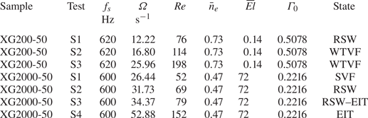
Additionally, some ‘steady-state’ experiments were performed in order to visualise specific flow states for longer times. For this type of experiment, the cylinder was first accelerated at  $\mathrm {d}\varOmega /\mathrm {d}t$ corresponding to a maximum acceleration rate
 $\varGamma _0$ until the targeted rotation speed/Reynolds number was reached, and the acquisition started. Details of such experiments are provided in table 3. The absence of polymer degradation was verified for all fluids by comparing the steady and oscillatory shear rheological characterisation made before and after the flow visualisation experiments. An example of such a comparison between pre-experiment and post-experiment rheological characterisations is available in the supplementary data for the XG2000-50 case (chosen as the most critical in terms of degradation probability, with its high polymer contribution to the viscosity and the strong shear rate at which it is employed during experiments).
Experimental conditions: steady-state experiments. Here  $\varGamma _0$ specifies the maximum non-dimensional acceleration rate used in the ramp-up leading to the recorded steady state.

3. Results
3.1. Overview of flow transitions
An overview of all flow states and ramp-up experiments is first presented. Each experiment starts from  $Re=0$ and
 $Re$ is progressively increased. Flakes align with dominant flow structures, reflecting light more or less intensely depending on their orientation, allowing one to capture various transitions to CF, TVF, WTVF, RSW, EIT and SVF. A space–time diagram, at constant
 $Re$, is provided for each flow state in figure 4(a–f). In TVF, SVF or WTVF, the flakes align with the (wavy/spiralling) Taylor vortices, giving rise to a band-like structure (figure 4a) that may be seen oscillating (figure 4b) or travelling (figure 4e) for WTVF and SVF, respectively. In RSW, the base TVF structure is still visible but additional patterns appear due to the local alignment of the flakes with axial elastic waves (figure 4c). In EIT, the random alignment of flakes with a set of various spatial flow structures translates into a chaotic intensity signal and space–time plot (figure 4d). Note that in CF, flakes are all aligned in the azimuthal direction, and the resulting space–time diagram is homogeneously grey (figure 4f).
Illustrative panel of observed flow maps and flow states. Panels (a–f) are space–time diagrams on  ${\rm \Delta} t$ intervals of 3 to 15 s spanning the
 $10 < z/d < 15$ vertical region: (a) N72,
 $Re=120$; (b) N72,
 $Re=250$; (c) P500-72,
 $Re=110$; (d) P500-72,
 $Re=150$; (e) XG2000-50,
 $Re=52$; (f) P500-72,
 $Re=50$. Panels (g) and (h) illustrate typical spatial and temporal spectra,
 $\mathrm {FFT}_s$ and
 $\mathrm {FFT}_t$, obtained by FFT processing along the vertical and horizontal dashed lines in panels (a–e), respectively.

Examples of spatial and temporal FFT (denoted as FFT $_s$ and FFT
 $_t$) of the space–time plots are shown in figures 4(g) and 4(h), as a function of the spatial wavelength and temporal frequency, respectively. These are computed along vertical and horizontal lines of panels from figure 4, respectively. The location of the peak(s) in these spectra, if present, can be used to determine the major spatial wavelength(s)
 $\lambda$ and temporal frequencies of the flow.
Figure 5(a) shows the succession of flow states encountered during several ramp-up processes (only one experiment per working fluid is shown for the sake of readability), in a three-dimensional space of elasticity, shear-thinning ( $1-\bar {n}_e$) and reduced Reynolds number (
 $Re/Re_0$), where
 $Re_0=107$ is the critical
 $Re_c^{TVF}$ Reynolds number for the CF to TVF transition for Newtonian fluids in the present set-up. A table summarising all critical Reynolds numbers for flow transitions is available in the supplementary data file. The results of Cagney et al. (Reference Cagney, Lacassagne and Balabani2020) have also been rescaled and added to the graph as dashed lines with the same colour code. Figures 5(b) and 5(c) are projections of figure 5(a) in (
 ${El},Re$) and (
 $1-\bar {n}_e, Re$) planes, respectively. The transition patterns are also summarised in table 2.
Summary of experiments in (a)  $(Re/Re_0,1-n_e,El)$, (b)
 $(Re/Re_0,El)$ and (c)
 $(Re/Re_0,1-n_e)$ parameter spaces. Each path corresponds to a single ramp-up experiment. Each flow state is associated with a line colour according to the legend (colours online). Full lines report experiments from the present work, and dashed lines experiments from Cagney et al. (Reference Cagney, Lacassagne and Balabani2020), performed in similar conditions (polymer batch, geometry, ramp-up protocol, flow visualisation method) on XG samples at various concentrations dissolved in a 25
 $\%$ glycerol in water solvent.

No clear trend appears from the two-dimensional projections; several regimes may coexist in some regions of the plots. For example, at  $Re=2\times Re_0$ and
 ${El}\sim 0.1$, the P500-72 experiment features EIT while the XG200-50 experiment is in the WTVF state for similar inertia and elasticity (figure 5b). Similarly, at
 $Re=2\times Re_0$ and for
 $1-n_e \sim 0.3$, XG1000-72 experiments feature EIT while XG200-50 is in the WTVF state, while at equivalent levels of inertia and shear-thinning (figure 5c). It is therefore necessary to consider all three parameters to distinguish preferential regions for each flow state in the three-dimensional parameter space, as done in figure 5(a). The WTVF can be found at high
 $Re/Re_0$, but only for intermediate elasticity. Conversely, EIT requires either strong elasticity or negligible shear-thinning to develop. The existing conditions of different flow states based on the rheological and inertial parameters are detailed and discussed in the rest of § 3.
3.2. Non-shear-thinning cases
3.2.1. Newtonian fluid
In the Newtonian reference case, the expected CF–TVF–WTVF transition pattern is retrieved, as illustrated in figure 6 with the N72-1 experiment. Prior to the onset of any instability, Ekman vortices (Cole Reference Cole1976) develop at the top and bottom of the cylinder (see e.g. figure 6b, top and bottom). The transition from CF to a band-like TVF structure can be clearly seen by a jump in the root mean square (RMS) value of the z-intensity profile 6(a), denoted  $i^*$. The CF to TVF transition occurs at
 $Re_c^{TVF}=107=Re_0$ and the transition from TVF to WTVF occurs at
 $Re_c^{WTVF}=218=2.03\times Re_0$. The latter, while difficult to observe on the flow map (figure 6b) due to a weak spatial amplitude, is clearly seen on the frequency map (figure 6c) when an additional frequency ridge appears. Both results are consistent with the values reported in the literature (see, for example, Dutcher & Muller (Reference Dutcher and Muller2009), Cagney & Balabani (Reference Cagney and Balabani2019b) and Ramesh, Bharadwaj & Alam (Reference Ramesh, Bharadwaj and Alam2019)), ranging from 80 to 120 and 170 to 450, respectively. The wavelength of TVF is
 $\lambda =0.89d$. The critical wavy frequency at the onset of the WTVF is
 $f_w=1.02\times f_{max}=1.40 \times ({\varOmega }/{2{\rm \pi} })$.
(a) Intensity signal, (b) flow map and (c) frequency map for the N72-1 experiment ( $\bar {{El}}=0$,
 $\bar {n}_e=1$). In panel (a) and all subsequent similar panels,
 $i^*$ is the RMS grey level intensity of panel (b) along the
 $z/d$ dimension, scaled by its maximum value on the
 $Re$ range. The dashed line on panel (c) denotes the inner cylinder rotation frequency
 $f_{\varOmega }$. Here
 $f_{max}$ is the rotation frequency corresponding to
 ${Re}_{max}$. Vertical dotted lines shows the transitions between flow regimes.

3.2.2. Boger fluid
In the Boger fluid case (P500-72), the transition pattern observed is CF–TVF–RSW–EIT (see figure 7). It is consistent with transitions reported in the literature for moderate or high elasticity fluids (Groisman & Steinberg Reference Groisman and Steinberg1996; Schaefer et al. Reference Schaefer, Morozov and Wagner2018). The onset of TVF happens at lower  $Re$ than in the Newtonian case,
 $Re_c^{TVF}=97=0.90\times Re_0$. Elastic waves (RSW) appear soon and abruptly after the onset of the TVF state, at
 $Re_c^{RSW}=103=0.96\times Re_0$, as several horizontal ridges become visible in the frequency map (figure 7c). These correspond to elastic waves, the frequency of which is not correlated to the Reynolds number but rather to the constant elastic number, through the elastic time scale (see Gillissen Reference Gillissen2019; Lacassagne et al. Reference Lacassagne, Cagney, Gillissen and Balabani2020). As a point of comparison, Dutcher & Muller (Reference Dutcher and Muller2013) reports transition to TVF at
 $Re_c^{TVF}/Re_0=1.07$ and to RSW at
 $Re_c^{RSW}/Re_c^0=1.13$ in moderately elastic Boger fluids (
 $El=0.1\text {--}0.2$). The apparent spatial wavelengths are
 $\lambda =0.82d$ and
 $\lambda =0.89d$ in TVF and RSW states, respectively, while Dutcher & Muller (Reference Dutcher and Muller2013) reported
 $\lambda \approx 1.6d$ in both states. The flow finally becomes increasingly disordered with
 $Re$, and quickly transitions to EIT at
 $Re$ values for which it would be laminar under purely inertial conditions.
(a) Intensity signal, (b) flow map (c) and frequency map for the P500-72-3 experiment ( $\bar {{El}}=0.19$,
 $\bar {n}_e=0.96$). The dashed line on panel (c) denotes the inner cylinder rotation frequency. Vertical dotted lines denote the transitions between flow regimes.

3.3. Shear-thinning dominated fluids
In the highly shear-thinning ( $\bar {n}_e=0.5766$) XG1000-25-1 case, a Newtonian-like transition pattern is observed: CF–TVF–WTVF (figure 8). A similar behaviour has been reported in several other studies where the fluid exhibited a non-negligible shear-thinning behaviour and negligible to moderate elasticity (Crumeyrolle et al. Reference Crumeyrolle, Mutabazi and Grisel2002; Cagney & Balabani Reference Cagney and Balabani2019a,Reference Cagney and Balabanib; Cagney et al. Reference Cagney, Lacassagne and Balabani2020). Here, it occurs despite the elastic number (
 $\bar {{El}}=1.2$) being approximately five times that of the fluid discussed in the previous section. Boger fluids of equivalent elastic number in the present experimental set-up are expected to exhibit elastic flow features such as RSW or transition to EIT, as suggested by experiment, reported above (§ 3.2.2). The absence of these in the flow map of figure 8 suggests that elastic effects are suppressed by shear-thinning. The CF to TVF transition occurs at
 $Re_c^{TVF}=72=0.67\times Re_0$. The flow is thus destabilised by combined shear-thinning and elasticity. The spatial wavelength of TVF is
 $\lambda =0.99d$, which is, as expected, slightly larger than that for the Newtonian case (Escudier et al. Reference Escudier, Gouldson and Jones1995; Cagney & Balabani Reference Cagney and Balabani2019b). The WTVF arises at
 $Re_c^{WTVF}=109=1.01\times Re_0$, again much sooner than in the Newtonian case. Moreover, at the onset of WTVF, the wave frequency is lower than the inner rotation frequency (
 $f_w=0.432 \times ({\varOmega }/{2{\rm \pi} })$) while it is higher in the Newtonian case. Finally, the complexity of the WTVF is enhanced, with ridges appearing and disappearing as
 $Re$ increases.
(a) Intensity signal, (b) flow map (c) and frequency map for the XG1000-25-1 experiment ( $\bar {{El}}=1.2, \bar {n}_e=0.58$). The dashed line on panel (c) denotes the inner cylinder rotation frequency. Vertical dotted lines denote the transitions between flow regimes. Note that the rotation frequency detected varies nonlinearly with
 $Re$, due to the shear-thinning behaviour (Cagney & Balabani Reference Cagney and Balabani2019b).

3.4. Elasticity dominated fluids
By keeping the same polymer at the same concentration (XG 1000 ppm) but simply increasing the solvent viscosity (XG1000-72-2 experiment), it is possible to produce a fluid of much higher elasticity ( $\bar {{El}}=13$) and weaker shear-thinning (
 $\bar {n}_e=0.71$). This fluid exhibits strikingly different patterns (figure 9). The flow abruptly transitions from CF to EIT, which is the typical behaviour of highly elastic fluids (Groisman & Steinberg Reference Groisman and Steinberg1996). This transition is easily detected from the abrupt jump in intensity RMS signal (figure 9a). No specific frequency can be identified in the flow map, as was also the case in the Boger fluid (figure 7) in the EIT state. The CF–EIT transition occurs at
 $Re_c^{EIT}=47=0.44\times Re_0$, which is in line with the results reported by Groisman & Steinberg (Reference Groisman and Steinberg1996): elasticity strongly destabilises the base Couette flow. While the latter is a well known result, the very different transition sequences in figures 8 and 9 constitute an interesting novelty of this study. Depending on the relative degrees of shear-thinning and elasticity dictated by the solvent properties, the flow of the same polymer at the same concentration may exhibit completely different hydrodynamic behaviours. Observations thus suggest that not only elasticity destabilises the flow, but it can also induce various hydrodynamic regimes by tuning the relative degrees of shear thinning and elasticity.
(a) Intensity signal, (b) flow map (c) and frequency map for the XG1000-72-2 experiment ( $\bar {{El}}=13$,
 $\bar {n}_e=0.71$). The dashed line on panel (c) denotes the inner cylinder rotation frequency. Vertical dotted lines denote the transition from CF to EIT. Note that the rotation frequency detected varies nonlinearly with
 $Re$, due to the shear-thinning behaviour, but this nonlinear trend is weaker than in figure 8(c), the shear-thinning index being here closer to 1.

3.5. Moderate shear-thinning and elasticity
Through changes in both solvent viscosity and polymer concentration, we can then keep a similar flow index ( $\bar {n}_e\approx 0.8$) and adjust the elasticity to be equivalent to that in the Boger fluid (
 $\bar {{El}}\approx 0.1$, figure 7, § 3.2.2), in order to probe the flow transitions in the moderate elasticity, moderate shear thinning regime of the parameter space (figure 5).
The behaviour (illustrated in figure 10, XG200-50-3 ramp-up experiment) approaches that of a fluid dominated by shear-thinning, with a Newtonian-like transition pattern, as shown in figure 8. The only notable difference is the existence of an intermediate RSW state between the TVF and WTVF states. The CF to TVF transition occurs at  $Re_c^{TVF}/Re_0=0.62$. The RSW waves appear at
 $Re_c^{RSW}/Re_0=0.67$ and completely disappear after
 $Re_c^{WTVF}/Re_0=0.83$. This RSW pattern bears some similarities with that exhibited by the Boger fluid (figure 7). However, shear-thinning seems to modify the nature of the RSW waves by enhancing their dependency on inertia, since the ridges are not completely
 $Re$-independent (figure 10c).
(a) Intensity signal, (b) flow map(c) and frequency map for the XG200-50-3 experiment ( $\bar {{El}}=0.14, \bar {n}_e=0.73$). The dashed line on panel (c) denotes the inner cylinder rotation frequency. Vertical dotted lines denote the transitions between flow states. Note that the rotation frequency detected varies nonlinearly with
 $Re$, due to the shear-thinning behaviour (Cagney & Balabani Reference Cagney and Balabani2019b).

Instead of EIT (as occurs for a Boger or elasticity dominated fluid), the flow transitions back to WTVF with increasing  $Re$. The WTVF state exists at
 $Re$ values lower than in the Newtonian case (
 $Re\simeq 100$), in line with the results for Newtonian-like shear-thinning fluids described in § 3.3. In order to investigate this specific RSW to WTVF transition further, steady-state experiments were performed on this fluid at three different
 $Re$ values:
 $Re=76$ (S1),
 $Re=114$ (S2) and
 $Re=198$ (S3) (see table 3). These are described in figure 11.
Steady-state recordings at constant  $Re$ of successive RIB and WTVF states for the XG200-50 case (
 $\bar {{El}}=0.14$,
 $\bar {n}_e=0.73$). (a–c) Space–time diagrams over 50 s time spans. (d–f) Close-ups of the same flow maps on the first 5 s and in the central region (dashed rectangles). (g) Spatial spectrum and (h) temporal spectrum of the three steady-state experiments.

The S1 case (figures 11a and 11d) displays an RSW pattern in which the base TVF structure is still visible, but periodic patterns are very pronounced. The frequency spectrum (figure 11h) clearly shows multiple peaks, with the highest energy peak found at  $f=0.33 \times ({\varOmega }/{2{\rm \pi} })$. The S2 case (figures 11b and 11e) lies between S1 and S3, with an evident WTVF structure; however, darker and whiter spots can be detected along given horizontal lines (figure 11e), indicating persisting RSW waves. The S3 case (figures 11c and 11f) shows a WTVF pattern similar to other reported shear-thinning WTVF states (figure 8, Cagney & Balabani (Reference Cagney and Balabani2019b)). The wavy frequency is lower than the inner cylinder frequency (
 $f_w=0.750 \times ({\varOmega }/{2{\rm \pi} })$ at
 $Re=198$, or
 $f_w=0.689 \times ({\varOmega }/{2{\rm \pi} })$ at
 $Re=150$ in figure 10(c). Multiple secondary peaks are visible, indicating a complex wavy behaviour. Cases S2 and S3 share a common peak at the same
 $f_w$ value when the frequency is scaled by
 $\varOmega$ (figure 11h). This peak is thus characteristic of an inertial flow feature, namely, WTVF. On the other hand, the lower frequency peak found in S1 at
 $f=0.33 \times ({\varOmega }/{2{\rm \pi} })$ is retrieved on S2 and S3 but progressively drifts towards higher frequencies with increasing
 $Re$ when the same scaling is used. This suggests that this other peak is not associated with inertia, but rather correlates with the elastic wave frequency (see figure 7, Lacassagne et al. (Reference Lacassagne, Cagney, Gillissen and Balabani2020)). This elastic feature (
 $f_w$ scaling with
 $t_e^{-1}$) progressively yields to inertia (
 $f_w$ scaling with
 $\varOmega$), as the flow gradually transitions from RSW to WTVF. The fact that the RSW ridges are not perfectly horizontal in the frequency maps suggests that, in shear-thinning fluids, both inertial and elastic effects are involved in the RSW pattern.
Further insight is brought by slightly shifting the fluids properties towards a more elastic, less shear-tinning case (XG200-72,  $\bar {{El}}=0.88$,
 $\bar {n}_e=0.85$). The transition pattern is then CF–TVF–RSW–EIT–WTVF, with an additional EIT state appearing (figure 12) between RSW and WTVF. The CF to TVF transition occurs at
 $Re_c^{TVF}/Re_0=0.43$. The RSW develops over a very limited
 $Re$ range, from
 $Re_c^{RSW}/Re_0=0.48$, quickly transitioning to EIT, and then smoothly to WTVF at
 $Re_c^{WTVF}/Re_0=1.0$. At
 $Re=150=1.4\times Re_0$ where the wavy frequency ridge is clearly visible on the frequency map (figure 12c), the wavy frequency is
 $f_w=0.451 \times ({\varOmega }/{2{\rm \pi} })$.
(a) Intensity signal, (b) flow map (c) and frequency map for the XG200-72-1 experiment ( $\bar {{El}}=0.88$,
 $\bar {n}_e=0.85$). The dashed line on panel (c) denotes the inner cylinder rotation frequency. Vertical dotted lines denote the transitions between flow states. Note that the rotation frequency detected varies nonlinearly with
 $Re$, due to the shear-thinning behaviour (Cagney & Balabani Reference Cagney and Balabani2019b).

This other fluid thus displays an elastic transition sequence (CF–TVF–RSW–EIT) until a sufficient amount of inertia ( $Re$) is reached, and the flow retransitions to a Newtonian-like behaviour, yet marked by shear-thinning. It is thus an extension of the previous case (XG200-50, figure 10) where elasticity plays a greater role in determining the nature of the transitions, as expected from the variations in rheological properties between the two fluids. It also leads to a counter-intuitive observation: the complexity of the flow and degree of chaos, induced by elasticity, can be reduced when increasing inertia together with shear-thinning. This intriguing behaviour cannot be attributed to polymer degradation, as rheological characterisation before and after confirmed the integrity of the polymer solutions. A possible explanation is the existence of an underlying damping mechanism of elastic waves with increasing inertia (
 $Re$).
Shear-thinning may compete with elasticity to condition the existence of elastic waves of flow patterns in the fluid (as previously observed by comparing figures 8 and 9), even to the point of relaminarising the flow (figures 10 and 12). Mild shear-thinning with moderate inertia allows elastic waves to exist, but high shear-thinning with moderate inertia (see the XG1000-25 case), or mild shear-thinning with higher inertia (XG200-50, XG200-72) do not.
3.6. Highly shear-thinning, highly elastic fluids
Experiments with a highly elastic and shear-thinning fluid (XG2000-50-2,  $\bar {{El}}=74$,
 $\bar {n}_e=0.56$) are reported in figure 13. The flow transition pattern is mostly elastic-like, with the final state being EIT (for
 $Re<300$). It is yet different from that of a Boger fluid, with an additional SVF pattern appearing between TVF and RSW. The transition sequence is thus CF–TVF–SVF–RSW–EIT. As expected from the strong elasticity and shear-thinning properties of the fluid, the CF destabilises at low-
 $Re$ values, and the onset of TVF occurs at
 $Re_c^{TVF}=37=0.34\times Re_0$. Elasto-inertial turbulence is reached at
 $Re_c^{EIT}=78=0.73\times Re_0$. The intermediate flow states therefore occur within a short Reynolds span. The transitions to RSW and EIT are close in
 $Re$ values, which compares well with the behaviour observed previously in the XG200-72 experiment (§ 3.5, figure 12).
(a) Intensity signal, (b) flow map and (c) frequency map for a highly elastic, highly shear-thinning fluid (XG2000-50-2 experiment,  $\bar {{El}}=74$,
 $\bar {n}_e=0.56$). The dashed line on panel (c) denotes the inner cylinder rotation frequency. Vertical dotted lines denote the transitions between flow states. Note that the rotation frequency detected varies nonlinearly with
 $Re$, due to the shear-thinning behaviour. Panel (d) is a close-up of panel (b) in the SVF state.

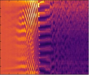
The additional SVF flow state corresponds to Taylor vortices spiralling and travelling along the axial direction, which translates on the flow maps as slanted dark and white stripes, not showing any particular temporal signature on the frequency map. The existence of such a flow state has been reported in elastic fluids (including the experiments of Baumert & Muller (Reference Baumert and Muller1997), linear stability analysis of Avgousti & Beris (Reference Avgousti and Beris1993)), solid particle suspensions (Ramesh et al. Reference Ramesh, Bharadwaj and Alam2019; Ramesh & Alam Reference Ramesh and Alam2020), but also Newtonian fluids with counter-rotating outer cylinder (Andereck et al. Reference Andereck, Liu and Swinney1986). Sudden changes of the spiralling propagation direction may occur and give rise to a similar flow state called the interpenetrating spiral vortex flow (ISVF) (Baumert & Muller Reference Baumert and Muller1997; Ramesh & Alam Reference Ramesh and Alam2020). In the recent works by Elçiçek & Güzel (Reference Elçiçek and Güzel2020a,Reference Elçiçek and Güzelb) SVF (sometimes coexisting with TVF) has also been observed in shear-thinning (possibly also elastic) XG solutions. Remarkably, SVF and ISVF have been found to coexist with RIB states under certain conditions (Ramesh & Alam Reference Ramesh and Alam2020). Indeed, RIB is actually the flow pattern resulting from the interactions between up-going and down-going stationary spirals of similar amplitudes. Latrache and coworkers (Latrache et al. Reference Latrache, Abcha, Crumeyrolle and Mutabazi2016) have shown that in shear-thinning and viscoelastic PEO solutions, a local reduction in the amplitude of either of the two spirals led to spatial defects, the multiplication of which was a mechanism for the transition to EIT. A subregion of the flow map in figure 13(b) in the (I)SVF state is shown in detail in figure 13(d). An SVF can be found to propagate either upwards or downwards. In highly shear-thinning XG solutions, it thus appears that one of the spirals can be completely suppressed, either on the full height of the cylinder (figures 13b, 13d, 14a (S1)), or locally (Elçiçek & Güzel Reference Elçiçek and Güzel2020b). The SVF or ISVF could thus be thought of as an alternative version of the RIB state, whereby shear-thinning combined with elasticity prevent spirals from coexisting everywhere in the gap.
Steady-state experiments in the SVF (S1), RSW (S2) and EIT (S3, S4) states, shown on  ${\rm \Delta} t$ intervals (horizontal axis) (the S1 interval is larger in order to better describe the SVF state). Superscripts ‘
 $-$’ and ‘
 $+$’ in S1 denote upward and downward spiralling velocities, respectively.

Complementary steady-state experiments have been performed and reported in table 3 and figure 14. This allows the spiral travelling speed to be computed for a constant  $Re=52$ value:
 $V_{SVF}=d\times \alpha$, where
 $\alpha$ (expressed in
 $\mathrm {s^{-1}}$) is the slope of isointensity lines on a time(normalised)–space flow map (time versus
 $z/d$, figures 4e and 14a). It is found that
 $V_{SVF}^-=-0.84\ \textrm {mm~s}^{-1}$ in the downward spiralling section of the steady-state experiment (figure 14, S1,
 $t<40~s$,
 $z/d < 15$, lower dashed line). In the upper right-hand corner of figure 14, S1, an upward spiralling region is observed, with
 $V_{SVF}^+=0.90\ \textrm {mm~s}^{-1}$ (dark dashed line). The very close magnitude of these two velocities suggests that SVF and RIB spirals are related, but that SVF corresponds to a bistable state, where a wave of given velocity may travel in either direction, while the RIB state requires both waves to coexist.
The steady-state experiment in the RSW state (at  $Re=69$, figure 14b), shows a pattern similar to that of the mild shear-thinning and elastic case XG200-50 in figure 11. With increasing
 $Re$, RSW state becomes increasingly disordered (figure 14c (S3)) and ultimately transitions to EIT (S4). In figure 15, the visualisation of figure 14c (S3)) is extended to a larger time span. Base Taylor vortices are crossed by multiple RSW waves, and the occurrence of several merge–split events and associated drifting of such base Taylor vortices are observed, leading to increased chaotic behaviours. Some merge–split and drifting features are indicated in figure 15 by dashed circles and lines, respectively. This merge–split transition (known as MST) is a mechanism of transition to EIT in elastic, Boger fluids (Lacassagne et al. Reference Lacassagne, Cagney, Gillissen and Balabani2020), and it appears that it also applies here in the case of a highly elastic but also shear-thinning fluid.
Steady-state experiment (30 s) showing the transitional stage between RSW and EIT in highly elastic and shear-thinning XG2000-50 fluid, at  $Re=79$: (a) reflected intensity; (b) binarised intensity map. Some of the numerous merging and splitting events of Taylor-vortices are highlighted by dashed circles, and the associated vortex drifting by dashed lines.

Finally, from the steady-state experiment above (figure 14), two-dimensional space–time spectra can be computed as a means to probe the spatio–temporal dynamics of EIT, in this case in a shear-thinning fluid. In the RSW state, a spatial peak exists at  $\lambda /d\sim 1$, due to the base TVF (figure 16a). In the temporal dimension, several clear peaks are identified, the most energetic found at frequencies much lower than the rotation frequency of the inner cylinder (figures 7c, 10c and 11h, Lacassagne et al. (Reference Lacassagne, Cagney, Gillissen and Balabani2020)).
Two-dimensional FFT (time and space) of steady-state experiments for the highly elastic, highly shear-thinning fluid (XG2000-50-2 experiment,  $\bar {{El}}=74$,
 $\bar {n}_e=0.56$) at (a)
 $Re=69$, (b)
 $Re=79$ and (c)
 $Re=152$ corresponding, respectively, to RSW, RSW transitioning to EIT, and EIT. Spectra are plotted in arbitrary units along a temporal frequency axis scaled by the inner cylinder rotation frequency
 $\varOmega /2{\rm \pi}$, and a spatial wavelength axis where the wavelength is scaled by the gap width
 $d$. Space-averaged and time averaged one-dimensional spectra are plotted in time-magnitude (blue) and space-magnitude (purple) planes, respectively. Vertical arrows are a guide to the eye showing peaks in both dimensions.

In the transitional RSW–EIT state (figure 16b) several peaks can be seen in the temporal spectra, albeit broader. The spatial peak corresponding to TVF is reduced in relative amplitude, and the most dominant one is found for  $\lambda /d < 1$. The spatial structure of the flow is no longer dominated by the Taylor-vortex wavelength, but by RSW waves of smaller wavelengths. Ultimately, EIT (figure 16c) displays smoother, broadband spectra of multiple spatial and temporal scales, which correspond well to the common definition of turbulence (Fenstermacher, Swinney & Gollub Reference Fenstermacher, Swinney and Gollub1979; Dutcher & Muller Reference Dutcher and Muller2013; Liu & Khomami Reference Liu and Khomami2013).
4. Discussion
In this section, the striking effect of shear-thinning mediation (attenuation and even suppression) of elastic flow patterns and EIT is discussed. First, the critical conditions for the onset of EIT in shear-thinning fluids are reported. Data from the present work and experiments from the literature are then compiled to derive an empirical criterion for EIT suppression in strongly shear-thinning fluids, and possible mechanisms for such behaviour are discussed.
4.1. Effect of shear-thinning on the transition to EIT
The transition to EIT, for some polymer solutions, is detected from the flow maps of ramp-up experiments. Values of all parameters at the critical point are denoted using the superscript  $EIT$ and subscript
 $c$. Note that while some parameters are constant throughout the ramp-up in Boger fluids (El, viscosity ratios, etc.) their value depends on the shear-rate-variable viscosity in shear-thinning fluids.
In figure 17(a), the critical value  $Re_c^{EIT}$ is plotted as a function of
 $1-\bar {n}_e$ with colours representing the magnitude of
 $\bar {{El}}$. At first, increasing the shear-thinning behaviour leads to a decrease in the critical
 $Re$ for the onset of EIT, with a simultaneous increase of elasticity. Above a critical shear-thinning index of 0.82 is reached (
 $1-\bar {n}_e=0.18$), shear-thinning appears to delay the onset of EIT, despite the simultaneous significant increase in
 $\bar {{El}}$ (figure 17a).
Critical Reynolds number value for the onset of EIT  $Re_c^{EIT}$ as a function of the (a) averaged shear-thinning index and (b) elastic number. Marker colours on panels (a) and (b) indicate the values of
 $\bar {{El}}$ and
 $1-\bar {n}_e$, respectively. Vertical lines are plotted at
 $n_e=0.82$ and
 $\bar {{El}}=1$ on panels (a) and (b), respectively, and those threshold values are also reported on the colour map of the conjugate figure (panels (b) and (a), respectively) as horizontal tick marks with arrows. Finally, panel (c) reports the critical values of
 ${El}$ at the onset of EIT,
 ${El}_c$, as a function of the critical shear-thinning
 $1-n_e$ also at the onset. Here
 $\bar {{El}}=1$ and
 $\bar {n}_e=0.82$ thresholds are noted as horizontal and vertical dashed lines, respectively.

A related non-monotonic trend can also be observed in figure 17(b) where  $Re_c^{EIT}$ is this time plotted against
 $\bar {{El}}$, with colour representing
 $1-\bar {n}_e$ values. For
 $\bar {{El}} < 1$, increasing
 $\bar {{El}}$ together with a moderate decrease in the shear-thinning index (
 $\bar {n}_e$ varying from 1 down to 0.82) leads to a decrease in
 $Re_c^{EIT}$. Further increase of
 $\bar {{El}}$ above unity, together with a significant increase of the shear-thinning property, is associated with a delay of EIT.
The elasticity versus shear-thinning parameter space thus seems to indicate the existence of a critical point at  $\bar {n}_e=0.82$ and
 $El\sim 1$. For
 $0.82>\bar {n}_e>1$, shear-thinning is not sufficiently strong to disrupt the elastic destabilisation of the flow and the triggering of EIT. However, for
 $\bar {n}_e<0.82$, even a large increase in elasticity is not sufficient to promote the onset of EIT, which is delayed by shear-thinning. In other words, for fluids with sufficiently strong shear-thinning rheology, the elastic instabilities are delayed by the shear-thinning behaviour. This trend can be seen by plotting the critical values of
 ${El}$ at the onset of EIT as a function of the critical values of
 $1-n_e$ at this same onset in figure 17(c). It is found that while
 $El < 1$ is sufficient to trigger elastic instabilities for
 $0.82>n_e>1$ (region R1 in figure 17(c), much higher values of
 ${El}$ (several orders of magnitude) are required for the onset of EIT if
 $n_e<0.82$ (region R2).
4.2. Suppression of EIT
Although EIT is found to be delayed due to shear-thinning (e.g. figure 13) in some experiments, it is not evidenced for  $Re<300$ in many other experiments reported here. Newtonian-like transition patterns (figure 8), or RSW transitioning to WTVF (figure 10) have been observed instead. In figure 18, data from the present study (circles for XG, square for PAAM) are plotted together with experiments from the literature in a shear-thinning versus elasticity parameter space
 $(1-\bar {n}_e,\bar {{El}})$. Experiments for which EIT has been reported in the Reynolds range measured (indicated in table 4) are denoted using white markers, while those for which EIT has not been observed (including the XG200-50 case with occasional RSW state, see figure 10) are denoted using black symbols. The flow transition patterns observed in these studies are also reported in table 4.
Shear-thinning versus elasticity parameter map in TCFs of polymeric solutions for the present study and literature experiments in the ( $1-\bar {n}_e, \bar {{El}}$) parameter space. White symbols indicate reported EIT and black ones the absence of it, for
 $Re < Re_{max}$ as reported in table 4. The flow transition patterns observed in these studies are also reported in table 4.

Flow transition patterns in shear-thinning and viscoelastic polymer or micellar solutions. Here N/A denotes quantities non-available or non-assessable from the available data.

It should be noted that the data from the literature are not always fully characterised. For example in Groisman & Steinberg (Reference Groisman and Steinberg1997), it is mentioned that the ‘apparent solution viscosity was decreasing with increasing shear rate’, but the degree of shear-thinning was not quantified. However, their solvent viscosity was sufficiently high for the fluid to exhibit mild shear-thinning at most, and their results are well within the moderate  ${El}$ range. A study involving WMS is also reported (Mohammadigoushki & Muller Reference Mohammadigoushki and Muller2017), for which we estimate the shear-thinning index from the steady-shear rheological characterisation reported by the authors (figure 1).
The  $(1-\bar {n}_e=0,\bar {{El}})$ axis of figure 18 shows the existence of a critical value for
 $\bar {{El}}$ beyond which EIT emerges for non-shear-thinning fluids. Below this curve, the transitions are Newtonian-like due to the weak elasticity. This threshold value increases with increased shear-thinning (increasing
 $1-\bar {n}_e$), so that for highly shear-thinning fluids, no EIT may be observed, even in the high-elasticity domain (figure 8). It may be attributed to the fact that EIT is completely suppressed by shear-thinning, or that it is simply delayed to
 $Re_c$ values beyond the range studied. From comparison with the literature (figure 18, table 4), it appears that this phenomenon is common to a variety of polymers (including PEO (Crumeyrolle et al. Reference Crumeyrolle, Mutabazi and Grisel2002; Latrache et al. Reference Latrache, Abcha, Crumeyrolle and Mutabazi2016), PAAM (Groisman & Steinberg Reference Groisman and Steinberg1996) and XG (Cagney et al. Reference Cagney, Lacassagne and Balabani2020), present study) and even to some extent to WMS (e.g. Mohammadigoushki & Muller Reference Mohammadigoushki and Muller2017). It becomes apparent that EIT needs both high
 ${El}$ and significant
 $Re$ to develop, but that shear-thinning may act to delay or even suppress elastic instabilities leading to EIT.
This can be expressed by an empirical criterion of the form
 \begin{equation} \bar{{El}} \gt {El}_c^0+K\times(1-\bar{n}_e)^\kappa,\end{equation}
where  ${El}_c^0=0.025$,
 $K=200$ and
 $\kappa =5$ are empirical parameters adjusted visually in order for the empirical line of (4.1) to separate the two domains (empty and full marker clouds) both in strong and weak shear thinning regions in figure 18. The first one corresponds to the
 ${El}$ threshold for Boger fluids, while the second and third ones describe the dependency of the
 ${El}$ threshold on the shear-thinning index. Discrepancies in the data, especially for moderate shear-thinning (
 $1-\bar {n}_e\sim 0.1$) and elasticity, may be attributed to the different geometrical parameters of the study reported (aspect ratio and radius ratio). It is indeed known that the streamline curvature has a great impact on the onset of purely elastic instabilities (Pakdel & McKinley Reference Pakdel and McKinley1996; Schaefer et al. Reference Schaefer, Morozov and Wagner2018), and could similarly affect elasto-inertial instabilities. The empirical constants are thus likely to be related primarily to those geometrical parameters, and physical parameter of the fluid (temperature, molecular weight, shear-thinning viscosity, viscosity ratio, etc.) embedded into the
 $\bar {{El}}$ and
 $\bar {n}_e$ estimators. On the other hand, figure 18, table 4 and (4.1) show that data collected from experimental set-ups with different various geometrical parameters, and using various polymer or micellar solutions, all follow this empirical behaviour. This could possibly suggest if not a universal behaviour, at least a weak influence of some of the geometrical parameters in the shear-thinning mediation process.
4.3. What are the mechanisms of shear-thinning mediation?
The mechanisms for mediation of elasto-inertial features by shear-thinning remain to be explained. Intuitively, one may first postulate that for strong shear-thinning, radial viscosity gradients exist within the gap due to the strong base azimuthal flow, leading to a low-viscosity inner core, and a high viscosity outer region. Viscous dissipation would then happen over a narrow range and an effective gap,  $d^r < d$, would exist, with
 $r_o^r < r_o$,
 $r_o^r$ being the outer radius of the flowing region. This is comparable to the flow of shear-banding solutions (Perge et al. Reference Perge, Fardin and Manneville2014).
The implications of this can be explored using simple scaling relations. Primarily, in the reduced gap, the apparent shear rate for a given rotation speed increases:  $\dot {\gamma }^r=\varOmega r_i/d^r>\dot {\gamma }$. As a direct consequence, the Weissenberg number is increased:
 \begin{equation} {Wi}^r=\dot{\gamma}^rt_e>{Wi}. \end{equation}
The apparent viscosity in the inner core (subject to higher shear rates  $\dot {\gamma }^r>\dot {\gamma }$) is expected to be lower than the apparent global viscosity in the full gap. Consequently, both the numerator and the denominator in the
 $Re$ definition are reduced as a result of the gap reduction (see (1.1)). Simplifying the viscosity shear-rate dependency to a power-law behaviour (introduced in § 1), one gets
 $\mu ^r \sim (\dot {\gamma }^r)^{n-1}$, with typically
 $-0.6 < n-1 < 1$. Since
 $\dot {\gamma }^r \sim 1/d^r$, it follows that
 $\mu ^r\sim (d^r)^{1-n}$,
 \begin{equation} Re^r \sim \frac{\gamma^r (d^r)^2}{\mu^r} \sim \frac{ (d^r)^{{-}1} (d^r)^2}{ ( (d^r)^{{-}1} )^{n-1} } \sim (d^r)^n \end{equation}
and, finally,
 \begin{equation} {El}\sim(d^r)^{{-}n-1}. \end{equation}
Since  $0 < n < 1$, shear-thinning will cause a decrease in d
 $^r$ which corresponds to a weak nonlinear decrease in
 $Re$, but more importantly an increase in El. Thus, shear-thinning is not likely to be the case of reduced elastic instability, since it is conversely expected to promote elastic properties (i.e. increase
 ${Wi}$,
 ${El}$).
While this analysis has been based on a purely azimuthal CF, the radial viscosity gradient due to the main shear in the gap persists even for higher-order flows. For example in Cagney & Balabani (Reference Cagney and Balabani2019b) and Topayev et al. (Reference Topayev, Nouar, Bernardin, Neveu and Bahrani2019), it is shown that Taylor vortices are squeezed and deform against the inner cylinder, in the lower viscosity inner region (Topayev et al. Reference Topayev, Nouar, Bernardin, Neveu and Bahrani2019). The previous scaling arguments on enhanced elasticity parameters are thus likely to hold in more complex flows as well due to the base mean shear. On the other hand, secondary flows such as Taylor vortices are also affected by shear-thinning (Cagney & Balabani Reference Cagney and Balabani2019b; Topayev et al. Reference Topayev, Nouar, Bernardin, Neveu and Bahrani2019), which in turn leads to axial viscosity gradients. Such axial viscosity gradients could well be involved in the damping effect of shear-thinning on transverse elastic waves. Results from § 3.5 also suggest that shear-thinning damping of elastic waves must involve an interplay between inertia and shear-thinning.
The effects of shear-thinning could thus be interpreted through a concept of preferential flow paths, outside of which elastic waves may not be able to travel. Axial elastic perturbations would thus be confronted with axial viscosity gradients which may act as dampers. Moreover, the strength of the extensional deformations induced by such perturbations would be reduced compared with the dominant radial shear rate, which is also in turn enhanced by the radial viscosity distribution. An analogy to this mechanism can be found in the recent work by Walkama, Waisbord & Guasto (Reference Walkama, Waisbord and Guasto2020), who performed an experimental study of the onset of elastic instabilities (at vanishing  $Re$) in a microfluidic flow of PEO-based Boger fluids past an array of cylinders. Spatial disorder was found to delay or even suppress the onset of elastic instability. This was explained by the establishment of preferential flow paths governed by the geometry, where shear deformation of the polymer is promoted over extensional deformation, having thus a stabilising effect on the polymer chains. Interestingly their results were also compared with a similar experiment using a shear-thinning 3000 ppm XG solution (which may have featured significant elasticity, however, not quantified). No elastic instabilities were observed on a similar range of
 ${Wi}$ values despite the zero spatial disorder imposed, suggesting that shear-thinning may act to suppress elastic disorder with mechanisms comparable to those of spatial disorder.
It should be mentioned that instabilities and flow transition in viscoelastic fluids are often found to be hysteretic and strongly subcritical (Groisman & Steinberg Reference Groisman and Steinberg1996; Martínez-Arias & Peixinho Reference Martínez-Arias and Peixinho2017). If one were to characterise the nature of the bifurcations, ramp-down experiments (decreasing inner cylinder rotation speed) would be needed. From the results of Martínez-Arias & Peixinho (Reference Martínez-Arias and Peixinho2017), there is no reason to expect shear-thinning to completely suppress hysteretic behaviours. It would yet be of great interest to see how the conclusions of the present study apply to flow states encountered specifically during ramp-down protocol only, such as diwhirls described in Groisman & Steinberg (Reference Groisman and Steinberg1996), Lange & Eckhardt (Reference Lange and Eckhardt2001) and Martínez-Arias & Peixinho (Reference Martínez-Arias and Peixinho2017).
5. Summary and conclusions
In this work, TCF of polymer solutions of various degrees of elasticity and shear-thinning were studied using flow visualisation. Combined shear-thinning and elasticity were found to globally destabilise the azimuthal Couette flow and favour the onset of unsteady flow states with increased complexity (WTVF, SVF), sometimes transitioning to chaotic and seemingly turbulent (RSW, EIT) even at relatively low  $Re$.
Shear-thinning mediates the transition patterns of moderately to highly elastic polymer solutions. In the absence of shear-thinning (Boger fluids), the flow transitioned to EIT even at moderate elasticity levels. In contrast, in highly shear-thinning cases, moderate to even high-elasticity fluids may undergo Newtonian-like transition patterns, for which no elasto-inertial instabilities occurred. Features of the flow states, such as the TVF wavelength or the wavy frequency were also modified by the fluid's rheology. When both shear-thinning and elasticity were moderate, elasto-inertial flow states (RSW, EIT) were reported in some cases. It was found that their nature was modified by shear-thinning. An increase in inertia tended to suppress chaos in the flow. Finally, in the most highly elastic fluids that also had significant shear-thinning, the flow ultimately did transition to EIT in a complex fashion. The MST mechanism reported in Lacassagne et al. (Reference Lacassagne, Cagney, Gillissen and Balabani2020) for Boger fluids was also observed. However, the transition occurred at elastic number values much higher than those required in the absence of shear-thinning.
The global effect of shear-thinning was, thus, to delay or even suppress elasto-inertial flow states, delaying their onset, occasionally damping chaotic features of the flow when inertia was increased, or even completely suppressing EIT. For this last effect, an empirical criterion for the existence of EIT was derived, also using results from the literature on various polymer solutions. Experiments with additional polymers, WMS, with a fully characterised rheology and in different geometrical configurations would be of great interest to verify the universality of this criterion. The physical origin of the shear-thinning mediation of elastic instabilities remains to be explained. It is not predicted by scaling arguments but could be the consequence of axial viscosity gradients caused by shear-thinning and secondary flows.
From a physical standpoint, both shear-thinning and viscoelastic properties originate from the same fluid component: polymer chains. Disentangling the two effects is extremely relevant from an empirical and applied point of view. It has, for example, recently been applied in order to explain flow phenomena in microfluidic devices (Casanellas et al. Reference Casanellas, Alves, Poole, Lerouge and Lindner2016; Haward et al. Reference Haward, Hopkins and Shen2020). Casanellas et al. (Reference Casanellas, Alves, Poole, Lerouge and Lindner2016) showed that in the absence of inertia, the Pakdel–McKinley criterion commonly used to describe the onset of purely elastic instabilities does not systematically capture the effects of shear-thinning. By properly characterising the fluid rheology, it may be possible to predict the existence, absence or damping of elasto-inertial regimes in a TCF without further knowledge or modelling of the state of polymer chains themselves. It is also evident that CF, TVF, WTVF or EIT may be associated with different degrees of mixing performances, related to flow unsteadiness and chaotic behaviour. Knowledge of very simple rheological fluid parameters could thus allow to foresee, for a given amount of inertia, the performance of a Taylor–Couette mixer in a shear-thinning and viscoelastic fluid. Tuning of such rheological parameters by controlling either the solvent viscosity or the polymer nature may in turn allow the mixing performances to be controlled and optimised.
Supplementary data
Supplementary data are available at https://doi.org/10.1017/jfm.2021.104.
Funding
Financial support for this work from the Engineering and Physical Sciences Research Council (EPSRC) Manufacturing the Future programme (no. EP/N024915/1) is gratefully acknowledged.
Declaration of interests
The authors report no conflict of interest.
Appendix. Effect of non-dimensional acceleration rate
In this Appendix, dedicated ramp-up experiments are performed. For each fluid, several tests are performed, in which  $Re_{max}$ is kept constant, and
 $\mathrm {d}\varOmega /\mathrm {d}t$ and experiment duration are varied over several decades to induce variations of
 $\varGamma _0$.
Five fluids corresponding to four different typical behaviours are studied: a Newtonian case (N72, noted N); a shear-thinning dominated case case, with a Newtonian-like transition sequence (XG1000-25, noted ST); a purely elastic, Boger fluid (P500-72, noted E); and a fluid with shear-thinning but dominant elasticity (XG2000-72, noted STE). Experimental conditions for all tests are detailed in table 5.
Experimental conditions: influence of ramp-up acceleration rate. Experiments are conducted for samples expected to exhibit different behaviours: Newtonian (N) figure 6; purely shear-thinning as described in figure 8 (ST) where elastic instabilities are suppressed by shear-thinning; purely elastic Boger fluid (E) (figure 7) with negligible shear-thinning; and shear-thinning dominated by elasticity (STE) figure 13. The superscript ‘*’ denotes experiments with  $\varGamma _0 < 1$ also reported in table 2.

The frequency map tool cannot be used in the following analysis. Indeed, when varying  $\mathrm {d}\varOmega /\mathrm {d}t$, the recording frequency has to be adapted in order to achieve similar
 $Re$-resolution flow maps regardless of the acceleration. In other words,
 $f_s/f_{max}$ has to be kept constant (typically above 3). Yet, the
 $N_c$ segment must be long enough to capture low-frequency events, even at high frame rates. Capturing a similar wave frequency
 $f_w$, with the same
 $f_s/f_{max}$ ratio, would require to increase
 $N_c$ proportionally to
 $f_s$ (in order of magnitude). The sampling time and
 $Re$ variations corresponding to
 $N_c$ may then become too large to assume that
 $Re$ stays constant within the sampled sequence. Frequency maps can thus not be used systematically to describe fast ramp-up experiments, and we are here limited to the qualitative study of flow states and to the quantification of transitions through flow maps. This is, however, a physical process more due to the acceleration rate itself rather than an experimental limitation: ramping up faster than a typical wave time scale does not allow a wave or perturbation with this time scale to develop in a steady manner, and thus to be captured in a frequency map.
In the Newtonian case (figure 19a), the flow maps are qualitatively similar for very different acceleration rates. However, the exact Reynolds number  $Re_c^{TVF}$ for the CF to TVF transition increases for the largest
 $\varGamma _0$. Values of
 $Re_c^{TFV}$ are plotted against
 $\mathrm {d}\varOmega /\mathrm {d}t$ and
 $\varGamma _0$ in figure 20, for all N runs in table 5 (along with the critical Reynolds number for the onset of WTVF,
 $Re_c^{WTVF}$, for the two lowest acceleration cases for which frequency maps can still be constructed). It appears that for
 $\varGamma _0 < 1$, the onset of TVF is not affected by the value of the acceleration rate as expected from the observations of Dutcher & Muller (Reference Dutcher and Muller2009).
Flow maps of fastest (top row) to lowest (bottom row) ramp-up experiments for (a) a Newtonian fluid, N; (b) shear-thinning fluid with a Newtonian-like transition, ST; (c) purely elastic Boger fluid, E; (d) shear-thinning fluid with strong elasticity, STE. The fluid type (N, ST, E, STE), run index (A to E) and maximum non-dimensional acceleration rate  $\varGamma _0$ are reported in each subpanel.

Values of critical Reynolds number for the onset of various flow states in the four investigated cases: Newtonian (N); shear-thinning with Newtonian-like transitions (ST); purely elastic Boger (E); and shear-thinning with elastic flow patterns (STE).

For the shear-thinning dominated case (figure 8), the flow maps are also not qualitatively affected. Note that in the fastest acceleration case, one can clearly identify the waviness of Taylor vortices just from the flow map. Figure 20 (ST) shows that for  $\varGamma _0<3$ the critical Reynolds number for CF to TVF transition does not depend on
 $\varGamma _0$.
The results for the purely elastic case are qualitatively different in terms of flow states transition. From figure 19(c), it appears that the RSW is modified by the variations in acceleration rates. The Reynolds range in which it can be found reduces with increasing  $\varGamma _0$, as illustrated in figure 20 where critical Reynolds numbers are plotted as a function of
 $\varGamma _0$. In the fastest acceleration case, it is difficult to tell whether the state observed from
 $Re=100$ to approximately
 $Re=120$ is TVF or RSW (this would require the use of frequency maps) but the flow signature is definitely different from low acceleration RSW. As in the N and ST cases, the onset of TVF is also delayed for high-
 $\varGamma _0$ values, and
 $Re_c^{TVF}$ can be assumed acceleration-independent for
 $\varGamma _0 < 1$. However, values of
 $Re_c^{EIT}$ are almost constant for all accelerations. This, in turn, leads to a narrowing of the Reynolds range left for the two intermediate regimes (TVF, RSW), i.e. regimes comprised between the base flow state (CF) and ultimate EIT. In other words, ramping up the inner cylinder at high-acceleration rates leads to a ‘squeezing’ of the intermediate transition steps in favour of an abrupt CF to EIT transition. Note that once again the ‘temporal’ frequencies (patterns along
 $Re$ axis) for RSW or EIT are more visible on the flow map in the fast cases, as the fast ramp-up leads to capture only a limited number of waves’ period, but describe them with great resolution, even though that description spans a significant
 $Re$ variation.
For the final case of a fluid where strong shear-thinning is dominated by elasticity (STE) we consider the XG2000-50 case studied previously (figures 13–16). Note that the XG1000-72 case has also been investigated and leads to results similar to the E case (Boger fluid (P500-72)). As in the E case, suppression of intermediate regimes (TVF, RSW, SVF) is reported. Contrary to the previous cases, however, the onset of the TVF flow is not affected as  $Re_c^{TVF}$ does not show any clear trend with
 $\varGamma _0$. On the other hand, it is the earlier onset of EIT that leads to the ‘squeezing’ of the intermediate Reynolds range.
From a qualitative point of view and in terms of succession of flow states, the N (Newtonian case (N72)) and ST cases are acceleration-independent, but E and STE fluids may have intermediate regimes suppressed for  $\varGamma _0\gg 1$. From a quantitative point of view, the CF to TVF transition is in general not affected by the acceleration rate for rates lower than unity (but higher acceleration rates may even be used in the ST case). To extend this acceleration study, it would be suitable to adapt the frequency maps analysis to highest acceleration rates, and adapt the dimensional acceleration rates to achieve constant non-dimensional acceleration rates throughout the ramp-up for shear-thinning fluids, as done in Dutcher & Muller (Reference Dutcher and Muller2013).