1. Introduction
Turbulent thermal convection is a phenomenon that occurs commonly in nature and in many industrial applications. Rayleigh–Bénard convection (RBC) is an idealised flow system involving heat transfer, which is a fluid contained within adiabatic sidewalls and horizontal conducting top-cooled and bottom-heated plates. In the RBC system, most of the temperature difference is sustained by thin thermal boundary layers over the conducting plates. Thermal plumes detach from the thermal boundary layers and self-organise into a quasi-two-dimensional large-scale circulation (LSC) in the bulk. Rayleigh–Bénard convection has been extensively explored in many experimental, numerical and theoretical studies (for reviews, see Kadanoff Reference Kadanoff2001; Ahlers Reference Ahlers2009; Ahlers et al. Reference Ahlers, Grossmann and Lohse2009; Lohse & Xia Reference Lohse and Xia2010; Chillà & Schumacher Reference Chillà and Schumacher2012).
Boiling is a very effective mode of heat transport and therefore it is used in various situations where a high heat removal rate from a surface is desired. The majority of research on the RBC system that examines a liquid–vapour phase change focuses exclusively on one fluid component (Oresta et al. Reference Oresta, Verzicco, Lohse and Prosperetti2009; Zhong et al. Reference Zhong, Funfschilling and Ahlers2009; Lakkaraju et al. Reference Lakkaraju, Schmidt, Oresta, Toschi, Verzicco, Lohse and Prosperetti2011; Schmidt et al. Reference Schmidt, Oresta, Toschi, Verzicco, Lohse and Prosperetti2011; Weidauer et al. Reference Weidauer, Pauluis and Schumacher2011; Biferale et al. Reference Biferale, Perlekar, Sbragaglia and Toschi2013; Urban et al. Reference Urban, Schmoranzer, Hanzelka, Sreenivasan and Skrbek2013; Weiss & Ahlers Reference Weiss and Ahlers2013; Zhang et al. Reference Zhang, Lhuissier, Sun and Lohse2014; Narezo Guzman et al. Reference Narezo Guzman, Fraczek, Reetz, Sun, Lohse and Ahlers2016a , Reference Narezo Guzman, Xie, Chen, Fernandez Rivas, Sun, Lohse and Ahlers2016b ; Hoefnagels et al. Reference Hoefnagels, Wei, Narezo Guzman, Sun, Lohse and Ahlers2017; Nakagawa & Sasa Reference Nakagawa and Sasa2017; Yang et al. Reference Yang, Howland, Liu, Verzicco and Lohse2023, Reference Yang, Chong, Liu, Verzicco and Lohse2024; Mouet et al. Reference Mouet, Michel, Pétrélis and Fauve2025). Boiling and droplet condensation during phase-change processes are recognised for significantly enhancing heat transport. However, studying RBC with phase changes is often difficult because filling an entire apparatus with specialised, low-boiling-point fluids is cost-prohibitive. Furthermore, vapour-bubble formation in these set-ups often relies on heterogeneous nucleation, a process that is notoriously hysteretic and difficult to replicate.
To address these challenges, Wang et al. (Reference Wang, Mathai and Sun2019) have introduced an innovative technique: using only a small amount of a secondary, highly volatile fluid to trigger the phase change within the primary system. The second fluid has a rather low boiling point
 $T_{cr}$
. Those authors applied a fixed temperature difference
 $\varDelta = T_{b} - T_{t}$
between the bottom (at
 $T_b$
) and the top (at
 $T_t$
) of the sample, with the mean temperature
 $T_{m}=(T_{b} +T_{t})/2$
chosen so that
 $T_{t}\lt T_{cr}$
while
 $T_{b}\gt T_{cr}$
. Heat absorption at the bottom plate triggers the formation of vapour bubbles that migrate towards the upper plate. Upon contact with the cooler surface, they condense into droplets and sink. These droplets and bubbles are known as bi-phasic particles since they consist of the second fluid in both its liquid and gaseous phases. By increasing the degree of superheat (
 $\Delta T_{\textit{sup}}\equiv (T_{b}-T_{cr})$
), the authors observed a linear enhancement of the Nusselt number. Ultimately, the study characterised how this heat transfer was influenced by the volume fraction of the second fluid.
The enhancement in heat transport is attributed to two primary mechanisms: the latent heat carried by the bi-phasic particles and the intensified turbulent mixing caused by their motion. Within the two-component RBC system containing bi-phasic particles, Wang et al. (Reference Wang, Mathai and Sun2020) identified a variety of flow structures distinct from standard plumes. Based on their gas-phase volume fraction and observed trajectories, these structures were categorised as full-vapour bubbles, bi-phasic risers, bi-phasic settlers or collective groups of bi-phasic particles. Such structural diversity offers new mechanisms for the precise manipulation of heat transport.
Understanding the physical mechanisms driving heat-flux enhancement in turbulent boiling flows remains a fundamental objective. In two-component RBC systems involving phase changes, the complexity increases significantly due to the expanded set of control parameters compared with traditional RBC. Consequently, investigating these systems across broader parameter ranges, such as lower Rayleigh numbers or conditions of constant ’supercold’ (maintained via a fixed top-plate temperature), is essential. Furthermore, in phase-change dynamics, the specific boiling and condensation temperatures emerge as critical parameters for system characterisation. In the present study, we investigate the dynamics of bi-phasic particles within a reduced-scale cylindrical sample. Using water and the low-boiling-point fluid HFE-7000, we explore a Rayleigh number regime one order of magnitude smaller than that of previous studies. While prior work by Wang et al. (Reference Wang, Mathai and Sun2019) maintained a constant Rayleigh number, thereby allowing superheat and supercold to vary, our approach utilises a fixed top-plate temperature. This configuration ensures a constant supercold, more closely mirroring the conditions found in industrial heat-exchange applications.
A primary objective of this study is to determine the physical limits of heat transport enhancement. While previous research has identified a linear relationship between enhancement, superheat and volume fraction, it remains unclear whether an upper bound exists. Our findings reveal superheat effects that diverge from prior results. By utilising visualisation techniques to interpret the global Nusselt number, this work provides new insights into how heat-flux enhancement functions as a global quantity under controlled conditions, particularly regarding its dependence on the superheat.
The remainder of this paper is organised as follows. In § 2 we define the parameters relevant to this system. Then, in § 3, we give a brief description of the apparatus used for the measurements. The results of heat transport and the motion of the particle are presented in § 4. A brief summary of the work is given in § 5.
2. Relevant parameters
For a single-phase fluid within a specific geometry, the system’s state is governed by two primary dimensionless variables. The first is the Rayleigh number (
 $\textit{Ra}$
), which represents the dimensionless temperature difference
 $\varDelta = T_{b} - T_{t}$
between the bottom (
 $T_{b}$
) and top (
 $T_{t}$
) plates:
 \begin{equation} \textit{Ra}=\frac {\alpha g \Delta H^3}{\kappa \nu }, \end{equation}
where
 $\alpha$
,
 $\kappa$
,
 $\nu$
and
 $g$
denote the isobaric thermal expansion coefficient, thermal diffusivity, kinematic viscosity and gravitational acceleration, respectively, and
 $H$
is the sample height. The second is the Prandtl number, defined as
 ${\textit{Pr}} = \nu / \kappa$
.
As HFE-7000 reaches its boiling point (
 $T_{cr}$
), it absorbs latent heat (
 $Q_{L}$
) to form vapour spheres governed by surface tension (
 $\sigma$
). To characterise the driving force for this phase change, we utilise the Jakob number (
 $\textit{Ja}$
). This parameter represents the ratio of available sensible heat to the energy required for vaporisation:
 \begin{equation} \textit{Ja}=\frac {\rho _{Hl}C_{\!pH,l}(T_b-T_{cr})}{\rho _{Hv}L}. \end{equation}
Here,
 $\rho _{Hl}$
and
 $C_{\!pH,l}$
are the density and specific heat capacity of liquid HFE-7000,
 $\rho _{Hv}$
is the vapour density and
 $L$
is the specific latent heat. The term
 $\Delta T_{\textit{sup}} \equiv (T_{b} - T_{cr})$
is defined as the bottom-plate superheat, while
 $(T_{cr} - T_{t})$
represents the top-plate subcooling (or underheat). In the present work,
 $\textit{Ja}\sim 1.4 \Delta T_{\textit{sup}}$
. These two quantities,
 $\textit{Ja}$
and the superheat, are of the same order. We used the superheat as a control parameter in the results section.
(a) Photo of the apparatus. (b) A diagram of the RBC cell. a, Bottom conducting plate; b, O-ring; c, HFE-7000 fluid; d, water; e, Plexiglas sidewall; f, top conducting plate; g, reservoir bottle; h, bottom thermal shield; i, side thermal shield. (c) Photo of the top plate. (d) Photo of the bottom plate of the cell.

Given the two-component nature of the system, we define an effective thermal conductivity (
 $\lambda _{\textit{eff}}$
) for the fluid layers in the conductive regime. The effective heat transfer coefficient is expressed as
 \begin{equation} \kappa _{\textit{eff}} \equiv (H/\lambda _{\textit{eff}})^{-1}=(h_{w}/\lambda _{w}+h_{H}/\lambda _{H})^{-1}, \end{equation}
where
 $\lambda _{w}$
and
 $\lambda _{H}$
are the thermal conductivities of water and liquid HFE-7000 and
 $h_{w}$
and
 $h_{H}$
are their respective equivalent heights. The HFE-7000 layer height is determined by its volume fraction,
 $h_{H} = \phi H$
. Consequently, the dimensionless vertical heat transport is quantified by the Nusselt number (
 $\textit{Nu}$
):
 \begin{equation} \textit{Nu}=\frac {Q}{A \kappa _{\textit{eff}} \Delta }, \end{equation}
where
 $Q$
is the heat flux and
 $A$
is the cell’s cross-sectional area.
In this study, HFE-7000 occupies a minimal volume fraction (
 $\phi = 0.86\,\%$
). Due to this small concentration, the bulk control parameters (
 $\textit{Ra}$
and
 ${\textit{Pr}}$
) are calculated using the physical properties of water. The error analysis in Appendix A shows that the estimation of
 $\textit{Ra}$
and
 ${\textit{Pr}}$
using the physical properties of water yields a negligible uncertainty. The primary departure from traditional RBC is the presence of bi-phasic particles. While the initial volume fraction
 $\phi$
is held constant, the vapour mass fraction, defined as
 $\beta _{V} \equiv m_{\textit{HV}}/m_{H}$
, serves as a critical response parameter. This value, representing the transition from liquid to gas phase, is experimentally determined by monitoring the liquid level displacement in a connected reservoir.
In the present work, three sets of eight thermistors are embedded at heights of
 $H/4$
,
 $H/2$
and
 $3H/4$
, respectively. The three layers are called the bottom, middle and top layers. Under the assumption of a quasi-two-dimensional LSC, the azimuthal temperature distribution
 $T_{i,k}$
at
 $\theta _{i,k}$
, where the indices
 $i$
and
 $k \in \{b, m, t\}$
denote the probe position and vertical stratum, respectively, is modelled via a first-order harmonic expansion. Specifically, the local temperature is projected onto a cosine profile of the form
 \begin{equation} T_{i,k} = T_{0,k} + \delta _{k} \cos (\theta _{i,k} - \theta _{k}), \end{equation}
where
 $T_{0,k}$
represents the mean bulk temperature,
 $\delta _{k}$
the flow strength of the LSC and
 $\theta _k$
the instantaneous azimuthal orientation of the roll structure at the corresponding elevation.
3. Apparatus and procedure
The experimental cell is a cylindrical vessel consisting of two horizontal copper plates coated with nickel and a transparent Plexiglas sidewall as shown in figure 1. The sample chamber has a height
 $H=18.70$
cm and a diameter
 $D=8.88$
cm, resulting in an aspect ratio
 $\varGamma = D/H = 0.50$
. To centralise the secondary fluid, the bottom plate features a concave surface with a curvature of
 $0.3\,\mathrm{ cm}^{-1}$
, causing the denser HFE-7000 to accumulate at the cell’s centre. To maintain a uniform fluid layer thickness across the radius, the top plate is designed with a matching convex surface of the same curvature. Thermal boundary conditions are maintained by a film heater attached to the bottom plate and a temperature-controlled water bath circulating through the top plate. Temperature precision is ensured by four thermistors embedded within each copper plate. Additionally, three layers of thermometers are integrated into the Plexiglas sidewall at heights of
 $H/4$
,
 $H/2$
and
 $3H/4$
to monitor the vertical temperature gradient. The assembly is secured using four metal rods that compress square metal laminas against the plates, with O-rings seated in precision-machined grooves to provide a hermetic seal between the conducting plates and the sidewall. The system utilises deionised water as the primary medium and HFE-7000 (3M Inc.) as the volatile secondary fluid. HFE-7000 is immiscible in water and possesses a low boiling point (
 $T_{cr}$
) at atmospheric pressure. For all experimental runs, the volume fraction of HFE-7000 was maintained at a constant
 $\phi = 0.86\,\%$
.
Following the assembly of the apparatus, deionised water was siphoned into the cell via a port at the perimeter of the top conducting plate. To introduce the secondary fluid, a plastic tube was inserted through the central port of the top plate, extending to the cell floor. A precise volume of HFE-7000 was then injected through this tube, ensuring it settled at the bottom. Once the fluids were loaded, the central and one peripheral port were sealed. The final peripheral port was connected via a thin capillary tube to a reservoir bottle partially filled with water. This reservoir serves as a volumeter; by monitoring the displacement of the water surface in the bottle, we can accurately measure volume changes within the sample during the experiment.
A significant challenge in this system is that air readily dissolves into HFE-7000, which can impede the condensation process. To remove dissolved air, a cyclic degassing procedure was implemented:
-
(i) Vaporisation: The bottom plate was heated to several degrees above the boiling point (
 $T_{cr}$
), while the top plate was maintained at
$5\,^{\circ }\mathrm{C}$
. This triggered the formation of bi-phasic HFE-7000 particles that cycled between the plates.
-
(ii) Air identification: Particles containing significant amounts of dissolved air failed to condense at the top plate, remaining trapped at the upper boundary as air bubbles.
-
(iii) Purging: After turning off the bottom-plate heater, the cell was tilted to collect these air bubbles at a peripheral port. Fresh deionised water was injected through a second port to displace the accumulated air through the outlet.


This procedure was repeated ten times over a 48-hour period. Successful degassing was confirmed when HFE-7000 consistently returned to the bottom plate, forming a stable, high-density film at the centre of the concave surface.
To ensure adiabatic conditions, the convection cell was enclosed within a thermal shield and positioned above a bottom thermal basin. The gaps between the cell, the shield and the basin were packed with insulating foam to minimise convective heat leakage. The thermal shield was actively regulated by a cooling water circuit to match the mean temperature of the fluid, while the thermal basin was maintained at the same temperature as the bottom plate. To accurately determine the heat flux through the fluid, we performed a calibration to account for residual heat losses and conduction through the Plexiglas sidewall. This was achieved by measuring the heat flow while the cell was filled with air. The resulting parasitic heat loss was then subtracted from the total power input to the bottom plate during the actual experiments to obtain the corrected Nusselt number.
Following the Nusselt number measurements, the thermal insulation, including the shield and foam, was removed to allow for optical access. A high-intensity white light beam was used to illuminate the cell, enabling the motion of the bi-phasic particles to be captured by a high-speed camera. For each experimental run, five separate image segments were recorded over a duration of approximately five minutes at a frame rate of 150 fps. To ensure the system had reached a statistical steady state, the final three video segments from each run were analysed. These segments consistently showed uniform flow behaviour, confirming the reliability and reproducibility of the observed structures.
In the present study, the top-plate temperature was maintained at a constant
 $10.00\,^{\circ }\mathrm{C}$
throughout all experimental runs. The initial run commenced with a bottom-plate temperature of
 $36.00\,^{\circ }\mathrm{C}$
. For each subsequent measurement, the time-averaged temperature of the bottom plate was increased in increments of
 $1.00\,^{\circ }\mathrm{C}$
to systematically explore the effects of varying superheat. For each specific temperature setpoint, the system was monitored over eight hours. Data from all thermistors and the power dissipation from the bottom plate were recorded at a high sampling frequency of approximately 0.24
 $\mathrm{ Hz}$
(one measurement every
 $4.17\ \mathrm{s}$
).To ensure that the calculated global heat transport reflects a true statistical steady state, the first hour of each recording was discarded as a transient period. Consequently, the final seven hours of data were utilised for time-averaging the temperatures and power, providing a robust basis for calculating the Nusselt number.
4. Results and discussion
4.1. The global heat transport efficiency
(a,b) The time traces of
 $T_b$
and
 $T_t$
and (c,d) the time traces of
 $Q_{\textit{tot}}$
. (a,c) Measurements taken for the superheat
 $\Delta T_{\textit{sup}}=-2 \,^{\circ }\mathrm{C}$
. (b,d) Measured for the superheat
 $\Delta T_{\textit{sup}}=10\,^{\circ }\mathrm{C}$
.

(a) The range of the condition
 $T_{m}$
and
 $T_{b}$
. (b) The ranges of parameters
 ${\textit{Pr}}$
and
 $\textit{Ra}$
for the experiment with pure water (blue squares) and with a mixture of water and HFE-7000 (black circles). (c) The Nusselt number as a function of the Rayleigh number on logarithmic scales. The dashed line is the power-law fitting to the data with both liquid-phase fluids,
 $\textit{Nu}=0.116Ra^{0.303\pm 0.009}$
. The dotted line is the GL model prediction,
 $\textit{Nu}=0.1143Ra^{0.306}$
. (d) Relative Nusselt number
 $\textit{Nu}_r$
as a function of the superheat
 $\Delta T_{\textit{sup}}$
. The dashed line is a linear function fitted to the data,
 $\textit{Nu}_r=0.118\times \Delta T_{\textit{sup}} + 1$
. Two solid lines are plotted at 0
 $\,^{\circ }\mathrm{C}$
and 2.7
 $\,^{\circ }\mathrm{C}$
.

Figure 3. Long description
Panel A: A scatter plot showing the relationship between T_b (bottom temperature in degrees Celsius) and T_m (midpoint temperature in degrees Celsius), T_t (top temperature in degrees Celsius), and T_b (bottom temperature in degrees Celsius). The x-axis represents T_b (°C), and the y-axis represents T_m, T_t, or T_b (°C). The plot includes three data series: black circles for T_m, blue triangles for T_t, and red circles for T_b. Panel B: A scatter plot showing the relationship between the Rayleigh number (Ra) and the Prandtl number (Pr). The x-axis represents Ra, and the y-axis represents Pr. The plot includes data points represented by black circles. Panel C: A scatter plot showing the relationship between the Rayleigh number (Ra) and the Nusselt number (Nu) on logarithmic scales. The x-axis represents Ra, and the y-axis represents Nu. The plot includes data points represented by black circles and red circles, with a dashed line for power-law fitting and a dotted line for the GL model prediction. Panel D: A scatter plot showing the relationship between the superheat (ΔT_sup in degrees Celsius) and the relative Nusselt number (Nu_r). The x-axis represents ΔT_sup (°C), and the y-axis represents Nu_r. The plot includes data points represented by black circles and red circles, with a dashed line for linear fitting and two solid lines at 0 and 2.7.
Representative temporal evolutions of the temperatures at top and bottom plates and the total heat flux are displayed in figure 2 for both the single-phase and the vapour-augmented HFE-7000 configurations. Following a brief transient, characterised by an initial overshoot in
 $T_t$
and damped oscillations in the total heat flux
 $Q_{\textit{tot}}$
, the system reaches a statistically stationary state at
 $t \approx 3000$
s. In this fully developed regime,
 $Q_{\textit{tot}}$
exhibits significant stochastic fluctuations about a well-defined time-averaged mean,
 $\langle Q_{\textit{tot}} \rangle _t$
. The statistically steady states can last for a duration exceeding 10 hours for both single-phase and the vapour-augmented cases. In the present experimental configuration, the spatially averaged temperature of each bounding plate is maintained at a constant value, rendering the corresponding thermal uncertainties negligible. The total measured heat flux
 $Q_{\textit{tot}}$
exhibits temporal fluctuations about its time-averaged mean, characterised by a standard deviation
 $\delta _{Q}$
. For both experimental runs, the relative fluctuation intensity is bounded at
 $\delta _{Q}/\langle Q_{\textit{tot}} \rangle _t \approx 2\,\%$
. A comprehensive uncertainty analysis, detailed in Appendix A, reveals that this ratio constitutes the primary source of experimental error. Consequently, the propagated uncertainty in the measured Nusselt number
 $\textit{Nu}$
, as well as the reduced Nusselt number
 $\textit{Nu}_r$
, is estimated to be approximately
 $2\,\%$
, as depicted in figures 3(c) and 3(d).
In the present work, the upper boundary is maintained at a constant temperature
 $T_t = 10\,^{\circ }\mathrm{C}$
. Consequently, the mean bulk temperature
 $T_m$
scales with the lower boundary temperature
 $T_b$
(figure 3
a), resulting in a simultaneous variation of the Rayleigh number (
 $\textit{Ra}$
) and Prandtl number (
 ${\textit{Pr}}$
), as illustrated in figure 3(b). This trajectory through the
 $(Ra, Pr)$
parameter space contrasts with the approach of Wang et al. (Reference Wang, Mathai and Sun2019), where
 ${\textit{Pr}}$
was varied at a fixed
 $\textit{Ra}$
. Then we examined
 $\textit{Nu}$
as a function of
 $\textit{Ra}$
when HFE-7000 remains liquid in the convection. As illustrated in figure 3(c),
 $\textit{Nu}$
exhibits a clear power-law dependence on
 $\textit{Ra}$
. Applying a power-law fit to the experimental data yields
 $\textit{Nu} \propto Ra^{\gamma _{\textit{eff}}}$
with an effective exponent of
 $\gamma _{\textit{eff}} = 0.303$
. This observed exponent is slightly smaller than the
 $\gamma _{\textit{eff}}^{GL} = 0.306$
predicted by the Grossmann–Lohse (GL) model for the corresponding
 $\textit{Ra}$
range and varying
 ${\textit{Pr}}$
(Stevens et al. Reference Stevens, van der Poel, Grossmann and Lohse2013). For equivalent values of the Prandtl number, the Nusselt number characterising the binary-liquid system is found to be consistently lower than that of the single-phase water baseline by 5.3 %. This reduction in the global heat transport efficiency is primarily attributed to the presence of HFE-7000; given that its thermal conductivity is significantly lower than that of water, the second phase effectively increases the thermal resistance of the boundary layers. As an illustrative example, we consider the physical properties of the fluids at
 $40\,^{\circ }\mathrm{C}$
from table 1, where the thermal conductivities of water and HFE-7000 are
 $\lambda _{w}=0.6297\,\mathrm{W\,m^{-1}\,K^{-1}}$
and
 $\lambda _{H}=0.072\,\mathrm{W\,m^{-1}\,K^{-1}}$
, respectively. To model this system, we assume that both fluids form flat, parallel layers on a flat conducting plate. Although this simplifies the actual physical configuration, it allows the layer heights to be expressed as
 $h_{w}=(1-\phi )H\approx 185.4$
mm for water and
 $h_{H}=\phi H\approx 1.6$
mm for HFE-7000. Under this assumption, the effective thermal conductivity
 $\lambda _{\textit{eff}}$
is determined by the series thermal resistance, given by (2.3) as
 \begin{equation} \lambda _{\textit{eff}}=\left (\frac {1-\phi }{\lambda _{w}}+\frac {\phi }{\lambda _{H}}\right )^{-1}. \end{equation}
For a representative volume fraction of
 $\phi = 0.86\,\%$
, the water and HFE-7000 resistance terms evaluate to
 $(1-0.0086)/0.6297=1.574\,\mathrm{W^{-1}\,m\,K}$
and
 $0.0086/0.072=0.1194\,\mathrm{W^{-1}\,m\,K}$
, respectively, yielding
 $\lambda _{\textit{eff}} = 0.591\,\mathrm{W\,m^{-1}\,K^{-1}}$
. This corresponds to a
 $6.2\,\%$
reduction relative to the thermal conductivity of pure water (
 $\lambda _w = 0.6297\,\mathrm{W\,m^{-1}\,K^{-1}}$
). Notably, this percentage decrease is consistent with the observed reduction in the Nusselt number. Consequently, HFE-7000 acts as a localised thermal insulator, suppressing the convective heat flux relative to the mono-phasic case. It should be noted that this calculation serves as an idealised approximation for an order-of-magnitude estimate, rather than a rigorous quantitative model, as the HFE-rich region is localised rather than uniformly distributed across the cell cross-section.
The physical properties of water and HFE-7000. The physical properties of water are adopted from Daubert & Danner (Reference Daubert and Danner1989). All the physical properties of HFE-7000 were provided by Rausch et al. (Reference Rausch, Kretschmer, Will, Leipertz and Fröba2015).

Table 1. Long description
A table comparing the physical properties of water and HFE-7000 at 40°C. The table has 11 rows and 4 columns. The columns are labeled Units, Water, HFE-7000 (liquid phase), and HFE-7000 (vapour phase). The rows are labeled with different physical properties and their respective values. Row 1: Thermal conductivity, W m^−1 K^−1, 0.6297, 0.072, 0.016. Row 2: Density, kg m^−3, 992.2, 1361.7, 9.5. Row 3: Specific heat, J kg^−1 K^−1, 416.9, 1300, 9.5. Row 4: Thermal diffusivity, m^2 s^−1, 1.53 x 10^−7, 4.07 x 10^−8, 1.36 x 10^−6. Row 5: Kinematic viscosity, M^2 s^−1, 6.69 x 10^−7, 2.6 x 10^−7, 1.36 x 10^−6. Row 6: Kinematic viscosity ratio, M^2 s^−1, 1, 0.39, 2.03. Row 7: Coefficient of thermal expansion, K^−1, 3.88 x 10^−4, 0.0022 at 25°C, 2.03. Row 8: Surface tension, 10^−3 N m^−1, 69.56, 10.27, 2.03. Row 9: Temperature coefficient, 10^−5 N m^−1 K^−1, 0.115, 2.03. Row 10: Specific latent heat of vaporisation, kJ kg^−1, 2257, 142, 2.03. Row 11: Prandtl number, 4.38, 6.39, 2.03.
Upon reaching the boiling point of HFE-7000 (
 $T_{cr} = 42\,^{\circ }\mathrm{C}$
), we observe an immediate linear growth in the Nusselt number as a function of both the superheat and the Rayleigh number. This initial enhancement is consistent with previous literature, which attributes the increased heat transport to the latent heat absorbed by HFE-7000 during the liquid–vapour phase change at the bottom plate. To quantify the impact of the bi-phasic particles, we define a relative Nusselt number,
 $\textit{Nu}_{r} = Nu / \textit{Nu}_{0}$
, where
 $\textit{Nu}_{0}$
represents the single-phase baseline established by the fit
 $\textit{Nu}_{0} = 0.116Ra^{0.303}$
. As shown in figure 3(d),
 $\textit{Nu}_{r}$
increases linearly with the superheat (
 $T_{b} - T_{cr}$
) at a rate of
 $k = 0.118$
. The linear dependence of the reduced Nusselt number
 $\textit{Nu}_r$
on the superheat
 $T_{b}-T_{cr}$
is consistent with the findings of Wang et al. (Reference Wang, Mathai and Sun2019). In the larger experimental cell considered by Wang et al. (Reference Wang, Mathai and Sun2019), and at higher Rayleigh numbers
 $\textit{Ra}$
, the supercooling varies concurrently with the superheat such that the temperature drops across the bounding plates remain invariant. For a volume fraction of
 $\phi =0.5\,\%$
, the linear growth regime of
 $\textit{Nu}_r$
observed in their study persists up to
 $\Delta T_{\textit{sup}} \lt 5^\circ \mathrm{C}$
, thereby spanning a broader parameter range than that observed in the present investigation. To evaluate the heat flux budget associated with the latent heat transport of HFE-7000, we consider an idealised regime where HFE-7000 vaporises completely at the bottom plate, advects to the top plate at a characteristic velocity
 $u_p$
and subsequently undergoes complete condensation. The additional heat flux
 $Q_{H}$
transported via this latent heat pathway may be modelled as
 \begin{equation} Q_{H} = \frac {\phi V_{\textit{cell}} \rho _{\textit{HL}} L_{H} }{H/u_{p}}, \end{equation}
where
 $L_{H} = 142\,\mathrm{ J\,kg}^{-1}$
is the specific latent heat of HFE-7000 (see table 1). For the case with superheat
 $T_{b}-T_{cr} = 2^\circ \mathrm{C}$
, Rayleigh number
 $\textit{Ra} = 4.8 \times 10^{9}$
and Prandtl number
 ${\textit{Pr}} = 5.83$
, the baseline heat flux through the water phase is estimated to be
 $Q_{w} \approx 70\,\mathrm{ W}$
. Taking the characteristic phase velocity to be
 $u_{p} \approx 5\,\mathrm{ cm\,s}^{-1}$
(the justification for which is detailed in § 4.2), the latent heat transport is evaluated as
 \begin{equation} Q_{H} = 0.0086 \times \pi (0.0444)^2 \times 0.187 \times 1361.7 \times 142 \times \frac {0.05}{0.187} \approx 0.515\ \mathrm{ W}. \end{equation}
This predicted value is approximately
 $0.007Q_{w}$
, which yields a heat transfer enhancement significantly smaller than the empirically observed Nusselt number ratio of
 $\textit{Nu}_r \approx 1.25$
for this run. This calculation yields an overestimation of both the characteristic velocity of HFE-7000 and the mass fraction actively participating in the phase-change cycle. Consequently, the contribution of the bi-phasic particle latent heat to the heat flux enhancement is expected to be less than 0.007. A secondary mechanism, enhanced turbulent mixing, likely accounts for a greater proportion of the heat transfer enhancement than the latent heat; however, quantifying this effect experimentally presents significant challenges.
A striking departure from previous studies occurs at a superheat of
 $\Delta T_{\textit{sup}} \gt 2.7\,^{\circ }\mathrm{C}$
. Beyond this threshold, the enhancement ceases its linear growth and reaches a plateau, with
 $\textit{Nu}_{r}$
maintaining a constant value of approximately
 $1.31$
. While the system returns to a power-law relationship with the same exponent as the single-phase regime, it operates with a significantly larger prefactor. This
 $31\,\%$
enhancement in heat transport is remarkably high, given that the HFE-7000 volume fraction is only
 $0.86\,\%$
. To our knowledge, this saturation effect has not been previously reported.
4.2. The morphology of bi-phasic particles
(a) Instantaneous snapshot of RBC with two liquids taken for the superheat
 $\Delta T_{\textit{sup}} =0\,^{\circ }\mathrm{C}$
. (b–g) Snapshots taken to show the boiling process of liquid HFE-7000 at the centre of the bottom plate.

Figure 4. Long description
Panel A: A photo showing a snapshot of Rayleigh-Bénard convection with two liquids. Panel B: A photo showing the initial state of the boiling process at 0 seconds. Panel C: A photo showing a tiny vapour bubble forming at 0.5 seconds. Panel D: A photo showing the growth of the vapour bubble at 1 second. Panel E: A photo showing the bubble further growing at 1.5 seconds with a scale bar indicating 5 millimeters. Panel F: A photo showing a bi-phasic particle at 2.5 seconds. Panel G: A photo showing the detaching of a big bubble at 2.98 seconds.
A localised enhancement in
 $\textit{Nu}$
is observed at the critical threshold
 $T_{cr} = 42\,^{\circ }\mathrm{C}$
, a phenomenon precipitated by the nucleation of bi-phasic (liquid–vapour) HFE-7000 structures (see supplementary movie 1 available at https://doi.org/10.1017/jfm.2026.12206). A representative snapshot of the system is depicted in figure 4(a), illustrating the boiling dynamics of HFE-7000 localised at the centre of the lower bounding plate. Several vapour embryonic structures or sessile bubbles with a characteristic radius of approximately 2 mm reside near the periphery of the plate, whereas a larger vapour mass with an equivalent radius of 5 mm is captured during its departure from the plate centre. Figure 4(b–g) tracks the temporal evolution of this detaching large vapour volume over a 3 s interval. Initially, as the lower-plate temperature exceeds the critical threshold
 $T_{cr}$
, localised vaporisation of the liquid HFE-7000 initiates at the centre, resulting in volume expansion and the encapsulation of a small internal bubble. This secondary bubble, possessing a radius of approximately 2 mm, escapes from the main vapour bulge at
 $t = 2.5$
s, followed by the complete detachment of the primary macro-bubble approximately 0.5 s later. This transition is consistent with the observations of Wang et al. (Reference Wang, Mathai and Sun2019).
For a given run, we time-average the greynesses of all the images during the statistically steady stage first. The time-averaged image is chosen as the background image to be subtracted from the image. Figure 5(a) displays an instantaneous background-subtracted visualisation at a superheat of
 $\Delta T_{\textit{sup}} = 2\,^{\circ }\mathrm{C}$
. The high-intensity gradients at the particle interfaces facilitate robust identification; specifically, the intense light scattering at the upper boundary of the structures reveals a distinct elliptic vapour pocket, confirming their bi-phasic morphology. The geometric characteristics of the bi-phasic structures are quantified by approximating the vapour (
 $i$
) and liquid (
 $o$
) phases as nested ellipsoids with semi-axes
 $(a_j, b_j)$
, as detailed in table 2. Under the assumption of transverse symmetry (i.e. a circular horizontal cross-section), the constituent volumes are determined via
 $V_{e,j} = ( {4}/{3})\pi a_{j}^{2}b_{j}$
for
 $j = i$
or
 $o$
. Utilising the phase-specific densities provided in table 1, the effective densities of the bi-phasic particles in figure 5(b,c) are calculated as
 $0.97\rho _{w}$
and
 $1.03\rho _{w}$
, respectively. These values indicate that the structures exist in a state of near-neutral buoyancy relative to the aqueous background. Notably, the particle volume remains invariant within the turbulent bulk; morphological transformations, such as expansion or contraction, are localised to the proximal region of the boundary where the thermal gradients are steepest.
The axes of the ellipses and the estimation of the density of bi-phasic particles in Figures 5(b) and 5(c).

Table 2. Long description
A table comparing dimensions and densities of bi-phasic particles in two figures. The table has 2 rows and 6 columns. The columns are labeled as follows: ai (mm), bi (mm), ao (mm), bo (mm), and rho (kg m^-3). Row 1: Figure 5(b), 2.2, 1.6, 2.8, 3.2, 968. Row 2: Figure 5(c), 2.8, 1.5, 3.7, 3.2, 1023.
(a) Instantaneous snapshot of RBC with two liquids taken for the superheat
 $\Delta T_{\textit{sup}} =2\,^{\circ }\mathrm{C}$
. (b,c) Enlarged images of two particles. The red oval marks the vapour part of the particle and the blue oval marks the bi-phasic particle. (d) The particles identified are marked in different colours.

Figure 5. Long description
Panel A: A grayscale image showing a cross-sectional view of a fluid convection system with numerous particles distributed throughout. The vertical axis is labeled Z in millimeters, and the horizontal axis is labeled X in millimeters. Panel B: An enlarged grayscale image of a single particle with a red oval marking the vapor part and a blue oval marking the bi-phasic part. Panel C: Another enlarged grayscale image of a single particle with similar red and blue oval markings. Panel D: The same cross-sectional view as in Panel A, but with particles identified and marked in various colors.
An automated segmentation algorithm (Jiang et al. Reference Jiang, Li, Ren, Liu, Zeng, Yu and Zhang2023) yields a population of approximately
 $N \approx 300$
particles, as illustrated by the colour-coded identifiers in figure 5(d). At this level of superheat, the vapour-phase expansion occupies a volume fraction of
 $0.2\,\%\times V_{\textit{cell}}$
, which is determined from the increase of the liquid in the reservoir. Assuming a spherical approximation, the mean characteristic diameter is estimated as
 \begin{equation} d_p \approx 2\times \left [ \frac {3}{4\pi } \frac {V_{\textit{cell}}(\phi + 0.2\,\%)}{N} \right ]^{1/3} \approx 4.3\,\mathrm{ mm}, \end{equation}
which is of the same order as the visual estimations of the particles in figures 5(b) and 5(c).
Within the bulk region of RBC, the flow field is characterised by buoyant plumes, coherent structures that detach from the thermal boundary layer. The plume is generally considered to have a size comparable to the thermal boundary layer. The characteristic thickness of this thermal boundary layer, denoted by
 $\delta _T$
, can be evaluated directly from the global heat transport efficiency, quantified by the Nusselt number
 $\textit{Nu}$
. By definition, balancing the conductive heat flux across the boundary layer with the total convective heat flux through the system yields the geometric relationship
 \begin{equation} \delta _T = \frac {H}{2 \textit{Nu}}. \end{equation}
For the present superheated state, the Rayleigh and Prandtl numbers are
 $\textit{Ra} = 4.8 \times 10^{9}$
and
 ${\textit{Pr}} = 5.83$
, respectively. Given a measured Nusselt number of
 $\textit{Nu} = 122.3$
and a cell height of
 $H = 0.1870$
m, the nominal thermal boundary-layer thickness is estimated as
 \begin{equation} \delta _T = \frac {187\,\mathrm{mm}}{2 \times 122.3} \approx 0.76\,\mathrm{mm}. \end{equation}
This is about the size of the thermal plume, which is smaller than the characteristic size of the bi-phasic particles. Crucially, the emitted plumes coalesce into a coherent LSC that ascends and descends adjacent to the vertical sidewalls. Experimental visualisations reveal that the particles remain uniformly distributed throughout the upper domain of the cell, suggesting that their spatial transport is not dominantly governed by the LSC. Beyond the discrete plumes and the mean LSC, the background turbulent fluctuations may also influence particle dynamics. However, since the present Rayleigh number is approximately two orders of magnitude lower than that investigated by Wang et al. (Reference Wang, Mathai and Sun2019), the characteristic impact of the background turbulence on the particles is correspondingly diminished.
In the following section, we analyse the spatial extent of the trajectories of bi-phasic particles to understand the enhancement of heat transport in the presence of the bi-phasic particles.
4.3. Distinct flow regions
(a) Instantaneous background-subtracted contrast-enhanced image of the flow with bi-phasic particles. (b) Image representing the standard deviation of the greyness of the system. (c) The dependence of the vertical position
 $z$
on the x-direction spatial-averaged greyness of the image in (b). The horizontal lines are the location of
 $Z_{\textit{int}}=92$
mm. (d) The time-averaged image, which is also used as the background image. The measurements of (a–d) were taken for the superheat 8.0
 $\,^{\circ }\mathrm{C}$
. (e) The vertical profile of the greyness of the background images taken for all five superheats. The profiles are shifted to the right by an increment of 30 with increasing superheat.

As shown in figure 6, background-subtracted and contrast-enhanced instantaneous images reveal a distinct spatial bias: the bi-phasic particles are primarily concentrated in the upper portion of the cylindrical cell. To quantify the occupancy of these particles, we generated a standard deviation map of the image greyscale (figure 6
b) for superheat
 $\Delta T_{\textit{sup}}=8\,^{\circ }\mathrm{C}$
from the expression
 \begin{equation} I_{\textit{rms}}(x,y)=\sqrt {\langle (I(x,y,t)-\langle I(x,y,t)\rangle _t)^2\rangle _t}, \end{equation}
where
 $\langle \cdots \rangle _t$
represents averaging quantities over time. While stationary elements like external wires and wall-adhered droplets remain visible, the moving bi-phasic particles appear as a bright, intensified region. This brightness directly correlates with the frequency and density of particle motion in the upper half of the sample. By calculating the spatially averaged greyscale intensity within the central region along the horizontal axis, figure 6(c) can map the vertical distribution of the particles into two regions. In the lower region (
 $Z \lt Z_{\textit{int}}$
), as the measurement moves away from the bottom plate, the image intensity increases very gradually. This suggests a relatively low density of vapour-rich particles in the lower bulk. At a specific height,
 $Z_{\textit{int}}$
, the intensity begins to rise sharply. This ‘interface’ marks the boundary where the bi-phasic particles become most prominent. In the upper region (
 $Z \gt Z_{\textit{int}}$
), the intensity gradient is significantly larger, peaking before decreasing slightly as the particles approach and condense at the top plate. In figure 6(c), two straight lines represent the linear functions fitting to the horizontal-spatial-averaged intensity. The intersection of lines determines the position of the ‘interface’
 $Z_{\textit{int}}$
. In the present experiment, the illumination of the apparatus is non-uniform, causing the time-averaged image to exhibit a strong dependence on the vertical coordinate, as shown in figure 6(d). Following an
 $x$
-direction spatial average, the vertical profiles of the image intensity for all five superheats (figure 6
e) exhibit an identical trend. Consequently, these profiles cannot be used to distinguish the spatial extent of the two-phase particle motion. The restricted spatial envelope of the particle trajectories persists across a range of superheats, specifically
 $\Delta T_{\textit{sup}} = \{2, 5, 8, 11, 14\}\,^{\circ }\mathrm{C}$
(see supplementary movies 2–6). Figure 7(a–e) presents instantaneous snapshots acquired at five distinct superheats. As the superheat increases, the spatial distribution of the particles contracts, becoming progressively localised within a narrower domain. These narrower domains are also observed from the standard deviation images in figure 7( f–j). To better quantify the range of particle movement, we average the greyness of the standard deviation images in figure 7( f–j) along the horizontal direction. The profiles of the averaged standard deviation greyness are shown in figure 7(k–o). The intersect of two linear fittings of greyness near the interface determines the position of the interface
 $Z_{\textit{int}}$
for each superheat. Within a given experimental realisation, the stochastic nature of the turbulent background precludes the existence of fixed ‘rebound’ coordinates for particles descending from the upper boundary. Consequently, to characterise the preferred spatial distribution of the bi-phasic structures, we transition from a Lagrangian tracking perspective to an Eulerian time-averaged representation. This averaging procedure filters the high-frequency interfacial fluctuations, allowing for a robust identification of the mean entrapment zones within the circulation.
(a)–(e) Instantaneous background-subtracted contrast-enhanced images of the flow with bi-phasic particles. ( f–j) Images of the standard deviation greyness. (k–o) The vertical profile of x-direction average greyness of the standard deviation images for different superheats. The images in each column are for the same superheat
 $\Delta T_{\textit{sup}}$
labelled at the top.

Figure 7. Long description
Panel A: Instantaneous background-subtracted contrast-enhanced image of the flow with bi-phasic particles at a superheat of 2.0°C. Panel B: Similar image at a superheat of 5.0°C. Panel C: Similar image at a superheat of 8.0°C. Panel D: Similar image at a superheat of 11.0°C. Panel E: Similar image at a superheat of 14.0°C. Panel F: Image of the standard deviation greyness at a superheat of 2.0°C. Panel G: Similar image at a superheat of 5.0°C. Panel H: Similar image at a superheat of 8.0°C. Panel I: Similar image at a superheat of 11.0°C. Panel J: Similar image at a superheat of 14.0°C. Panel K: Line graph showing the vertical profile of x-direction average greyness of the standard deviation images at a superheat of 2.0°C. The y-axis represents height in millimeters, and the x-axis represents greyness intensity. Panel L: Similar line graph at a superheat of 5.0°C. Panel M: Similar line graph at a superheat of 8.0°C. Panel N: Similar line graph at a superheat of 11.0°C. Panel O: Similar line graph at a superheat of 14.0°C.
(a) The location
 $Z_{\textit{int}}$
as a function of the superheat. The curve is a third-order polynomial function fitted to the data. The coefficients are −13.9, 2.9, 2.32 and −0.1216 for the terms of order 0,
 $\ldots$
, 3. (b) The height ratio of the two regions
 $h_{i}/H$
for i = 1 (diamond) and i = 2 (circle).

The transition height,
 $Z_{\textit{int}}$
, effectively partitions the sample into two distinct hydrodynamic regimes. The lower region (
 $z \lt Z_{\textit{int}}$
) consists of single-phase water, while the upper region (
 $z \gt Z_{\textit{int}}$
) is characterised by a high concentration of vigorously moving bi-phasic particles. This stratification contrasts with the findings of Wang et al. (Reference Wang, Mathai and Sun2019), where bi-phasic particles were observed to travel the full height of the cell from the bottom plate to the top plate. In our system, the effective travelling distance of the bi-phasic particles is restricted and can be defined as
 \begin{equation} h_{2} = H - Z_{\textit{int}}. \end{equation}
The variation of
 $Z_{\textit{int}}$
relative to the degree of superheat is shown in figure 8(a). We observe a nonlinear relationship. At a superheat of approximately
 $2\,^{\circ }\mathrm{C}$
, the particles span the entire cell (
 $Z_{\textit{int}} \approx 0$
), behaving similarly to that in previous studies. As the superheat rises,
 $Z_{\textit{int}}$
increases, meaning the bi-phasic particles are confined to a shrinking upper region. Consequently, the effective travelling distance
 $h_{2}$
decreases as the system is driven harder as shown in figure 8(b). To quantify this behaviour, the data for
 $Z_{\textit{int}}$
as a function of superheat
 $\Delta T_{\textit{sup}}$
were fitted using a third-order polynomial:
 \begin{equation} Z_{\textit{int}} = a_{0} + a_{1} \Delta T_{\textit{sup}} + a_{2}(\Delta T_{\textit{sup}})^2 + a_{3}(\Delta T_{\textit{sup}})^3, \end{equation}
with the following coefficients:
 $a_{0} = -13.9$
,
 $a_{1} = 2.9$
,
 $a_{2} = 2.32$
and
 $a_{3} = -0.1216$
. This trend suggests that as the temperature of the bottom plate increases, the physical space in which the phase-change particles effectively transport heat becomes increasingly restricted to the upper portion of the cell.
(a) The time-averaged and azimuthally spatially averaged temperature at different heights against the superheat
 $\Delta T_{\textit{sup}}$
. (b) The normalised temperature at different heights
 $T_{n}(z)\equiv (T(z)-T_t)/(T_b-T_t)$
against the superheat. (c) The temperature drops
 $\Delta _{bm}\equiv T(H/4)-T(H/2)$
and
 $\Delta _{mt}\equiv T(H/2)-T(3H/4)$
against the superheat. (d) The normalised temperature drops
 $\varDelta _{bm}/\varDelta$
and
 $\varDelta _{mt}/\varDelta$
against the superheat.

Because the particulate phase is localised within a specific subdomain of the system, it is instructive to examine whether the vertical temperature distribution reflects this spatial variation in the working fluid composition. Figure 9(a) depicts the temperature measurements at various heights as a function of the superheat,
 $\Delta T_{\textit{sup}}$
. While all three temperature signals increase monotonically with
 $\Delta T_{\textit{sup}}$
, a distinct reduction in the gradient
 $\mathrm{d}T/\mathrm{d}\Delta T_{\textit{sup}}$
is observed following the onset of bi-phasic particle formation. For
 $\Delta T_{\textit{sup}} \gt 5\,^\circ \mathrm{C}$
, the temperature gradient at
 $H/4$
increases, which is attributed to the absence of particle sedimentation to this depth. Similar trend shifts are manifested at alternative elevations. Crucially, the critical superheat at which these gradient transitions occur scales positively with the vertical coordinate, confirming that the local structural modification of the temperature profile is driven by the spatial boundary of the bi-phasic particulate region. The vertical temperature differences between adjacent measurement planes, defined as
 $\varDelta _{bm} \equiv T(H/4) - T(H/2)$
and
 $\varDelta _{mt} \equiv T(H/2) - T(3H/4)$
, are presented in figure 9(c). In the single-phase regime (
 $\Delta T_{\textit{sup}} \lt 0\,^\circ \mathrm{C}$
), where bi-phasic particles are absent,
 $\varDelta _{mt}$
remains invariant at approximately
 $1\,^\circ \mathrm{C}$
. Beyond a critical superheat of
 $\Delta T_{\textit{sup}} \gt 4\,^\circ \mathrm{C}$
,
 $\varDelta _{mt}$
increases progressively until it saturates at
 $1.3\,^\circ \mathrm{C}$
for
 $\Delta T_{\textit{sup}} \gt 10\,^\circ \mathrm{C}$
. This asymptotic behaviour closely mirrors the saturation observed in the global Nusselt number. The lower temperature difference,
 $\varDelta _{bm}$
, exhibits a qualitatively identical trend but is amplified by a factor of approximately 1.5 relative to
 $\varDelta _{mt}$
. Furthermore,
 $\varDelta _{bm}$
achieves its asymptotic plateau at a lower superheat threshold of
 $\Delta T_{\textit{sup}} \approx 8\,^\circ \mathrm{C}$
. To elucidate the thermal gradient across each discrete subregion, the normalised temperature profiles, defined as
 $T_n = (T - T_t)/\varDelta$
, are plotted in figure 9(b). When the system is entirely occupied by the liquid phase, the normalised temperatures at all three elevations increase with
 $\Delta T_{\textit{sup}}$
, indicating an enhanced thermal resistance across the top boundary layer. Following the phase change of the HFE-7000 component, all normalised temperatures decrease with increasing superheat. As the superheat is elevated further and the internal phase interface migrates upward, the normalised temperature at the lower boundary,
 $T_n(H/4)$
, establishes a temporary plateau before decreasing further. This structural shift in the slope is replicated at higher elevations, albeit delayed to progressively larger values of superheat. Within the bulk region, the normalised temperature gradient between the lower two measuring stations consistently exceeds that of the upper pair. Finally, although non-uniformities exist in the localised internal temperature drops, they collectively constitute less than 6 % of the total temperature differential across the entire convective cell, as demonstrated in figure 9(d).
Drawing an analogy to a two-layer RBC system, we can model the sample as two distinct thermal regions separated by the interface at
 $Z_{\textit{int}}$
. A critical step in understanding the heat transfer across this boundary is determining the local temperature at the interface. As reported by Wei & Ahlers (Reference Wei and Ahlers2014, Reference Wei and Ahlers2016), the vertical temperature profile within the quasi-isothermal bulk of classical RBC is well characterised by a logarithmic distribution, whose coefficients exhibit a spatial dependence on the radial distance from the cell axis. In the present study, there are only three spatially averaged temperature measurements at discrete heights along the lateral boundary. Consequently, a logarithmic fit to the local temperature field is mathematically underdetermined. Furthermore, because the interface separating the two regions is neither fixed in space nor strictly isothermal, we estimate the fluid temperature at the interfacial height
 $Z_{\textit{int}}$
via linear interpolation of the vertical temperature profile recorded by the thermistors embedded in the sidewall. As illustrated in figure 10(a), the vertical temperature distribution along the bounding sidewall deviates from a linear profile within the bulk region of the domain. To achieve a more accurate determination of the internal interface temperature,
 $T_{\textit{int}}$
, a localised piecewise interpolation/extrapolation scheme is employed. Specifically,
 $T_{\textit{int}}$
is estimated using either the two lower-region measurements,
 $T(H/4)$
and
 $T(H/2)$
, or the two upper-region measurements,
 $T(H/2)$
and
 $T(3H/4)$
. The resulting interface temperatures from these localised evaluations are denoted by stars in figure 10(a). For comparison, the interface temperature is also evaluated via a global polynomial fit utilising all three temperature data points simultaneously, as demonstrated in figure 10(b). The discrepancy between the interface temperatures obtained from these two estimation methodologies, defined as
 $\delta T_{\textit{int}}$
, varies boundedly from
 $-0.2\,^\circ \mathrm{C}$
to
 $0.3\,^\circ \mathrm{C}$
(see figure 10
c). This variation is small in magnitude, constituting less than 1 % of the total temperature difference across the cell,
 $\varDelta$
, as quantified in figure 10(d).
(a) Time-averaged temperatures of three vertical positions for all the runs in the present work. From left to right, the superheat of each run increases by 1
 $\,^{\circ }\mathrm{C}$
from −6
 $\,^{\circ }\mathrm{C}$
to 15
 $\,^{\circ }\mathrm{C}$
. The runs with superheat
 $\Delta T_{\textit{sup}}\lt 0$
are plotted with open symbols. The red symbols represent the runs where the interface is located at the lower half of the system. The blue symbols represent the runs where the interface is located at the upper half of the system. The stars are the fitted temperature of the interface fitted from the nearest two temperatures along the sidewall. (b) The fitted temperatures of the interface against the superheat
 $\Delta T_{\textit{sup}}$
. The filled symbols are fitted from all temperatures at different heights along the sidewall. The open symbols are fitted from only two nearest temperatures around the interface. The right axis shows the difference
 $T_{\textit{int}} - T_{cr}$
. (c) The difference of the interface temperatures fitted by two different methods
 $\delta T_{\textit{int}}$
against the superheat. (d) The normalised temperature differences
 $\delta T_{\textit{int}}/\varDelta$
against the superheat.

Figure 10. Long description
Panel A: A line graph showing time-averaged temperatures at three vertical positions for various runs. The x-axis represents temperature in degrees Celsius, and the y-axis represents the normalized height. Different symbols and colors indicate different superheat levels and interface positions. Panel B: A scatter plot showing fitted interface temperatures against superheat. The x-axis represents superheat in degrees Celsius, and the y-axis represents interface temperature in degrees Celsius. Filled and open symbols differentiate fitting methods. Panel C: A scatter plot showing the difference in interface temperatures fitted by two methods against superheat. The x-axis represents superheat in degrees Celsius, and the y-axis represents the temperature difference in degrees Celsius. Panel D: A scatter plot showing normalized temperature differences against superheat. The x-axis represents superheat in degrees Celsius, and the y-axis represents normalized temperature differences.
The evolution of
 $T_{\textit{int}}$
relative to the bottom-plate superheat reveals an interesting thermal behaviour. As the superheat increases,
 $T_{\textit{int}}$
initially decreases before trending upward again. Despite these fluctuations,
 $T_{\textit{int}}$
remains within a narrow window between
 $29.5\,^{\circ }\mathrm{C}$
and
 $31.3\,^{\circ }\mathrm{C}$
. Significantly, this temperature range is approximately
 $10\,^{\circ }\mathrm{C}$
lower than the boiling point (
 $T_{cr} = 42\,^{\circ }\mathrm{C}$
). This suggests that the bi-phasic structures subsist at temperatures below the nominal boiling point. The persistence of a metastable vapour phase under such subcooled conditions remains a non-trivial observation, necessitating high-resolution local temperature measurements of the dispersed phase to elucidate the stabilisation mechanisms and the resulting kinematic confinement.
(a) From bottom to top, temperatures measured at the top (at a height of
 $H/4$
), middle (
 $H/2$
) and bottom (
 $3H/4$
) layers at the sidewall as a function of
 $\theta$
. Lines are cosine functions fitting to the data. (b) The time series of the azimuthal orientation of the LSC
 $\theta _k$
. (c) The time series of normalised flow strength
 $\delta _k / \langle \delta _k \rangle$
at each layer. The line represents the value of 0.15. The measurements are taken for the superheat
 $\Delta T_{\textit{sup}} = 6\,^{\circ }\mathrm{C}$
.

In the RBC with
 $\varGamma = 0.5$
, the primary LSC typically undergoes a bifurcation into a stacked two-roll structure, driven by turbulent fluctuations at elevated Rayleigh numbers (Xi & Xia Reference Xi and Xia2008). A transition between the single-roll and double-roll topologies of the LSC induces a variation in the Nusselt number of approximately 2 %. Furthermore, the spatial morphology of the LSC is expected to profoundly influence the transport and distribution of the bi-phasic particulate phase. Consequently, we characterise both the structural configuration of the LSC and its associated azimuthal dynamics. Conversely, the present results indicate that the LSC maintains a coherent single-roll topology throughout the parameter space investigated. Figure 11(a) illustrates the instantaneous azimuthal temperature distributions at three layers for the superheat
 $\Delta T_{\textit{sup}}=6\,^{\circ }\mathrm{C}$
. The temperature signals are found to be well approximated by first-order harmonic (cosine) fits, with the azimuthal phase,
 $\theta _k$
, exhibiting strong alignment across the bottom, middle and top layers. This phase coherence, coupled with the persistent non-zero magnitude of the equatorial flow strength,
 $\delta _m$
, supports the characterisation of the LSC as a quasi-two-dimensional structure spanning the entire cell height. A transition to a vertically partitioned two-roll state would be marked by a vanishing middle flow strength,
 $\delta _m \to 0$
. However, as shown in the normalised time series
 $\delta _m/\langle \delta _m \rangle$
(figure 11
c), the flow strength remains predominantly above the cessation threshold of
 $0.15$
. In the present experimental run, a total cessation of the LSC, defined as the condition wherein the local flow strength across all three measurement planes falls below
 $0.15\langle \delta _k\rangle$
simultaneously, was not detected. A temporally localised cessation observed exclusively at either
 $H/4$
or
 $3H/4$
signifies that a single-roll state (SRS) is confined to the lower or upper hemisphere of the cylindrical cell, respectively. Conversely, a localised cessation occurring solely at the mid-height plane (
 $H/2$
) denotes the presence of a double-roll state (DRS), characterised by two counter-rotating, vertically stacked rolls. For the present configuration, this DRS manifests periodically with an average recurrence interval of approximately 1 hour and a typical lifetime of 20 s. Following the dissolution of the DRS, the LSC collapses back into a globally coherent SRS at its original azimuthal orientation. At a Rayleigh number of
 $\textit{Ra} = 5.93 \times 10^9$
, the cumulative time fraction occupied by the DRS is merely 0.6 %. A corresponding analysis was performed for the reference regime where the HFE-7000 component remains entirely in the single-phase liquid state (at subsaturation conditions,
 $\Delta T_{\textit{sup}} \lt 0^\circ \mathrm{C}$
). In this regime, both the SRS and DRS topologies are again present, with the DRS similarly accounting for approximately 0.6 % of the total duration. This statistical occupancy is significantly lower than the value reported by Weiss & Ahlers (Reference Weiss and Ahlers2011), who observed a DRS time fraction of approximately 10 %. This order-of-magnitude discrepancy is hypothesised to arise from the geometric stabilisation induced by the curved conducting boundary plates utilised in the current experimental apparatus. Instances of localised LSC collapse are rare, even upon the introduction of bi-phasic particles. We conclude that the single-roll LSC remains robust against both the turbulent background and the secondary phase perturbations. Consequently, the observed spatial confinement of the bi-phasic particles cannot be attributed to a structural reorganisation of the global circulation.
In this section, we highlight the anomalous behaviour of the bi-phasic particles, which challenges the established models of two-component boiling convection. The most surprising findings in this work concern the spatial range of particle movement and the thermal environment they inhabit. We observe three key distinctions from previous research, namely the range of particle movement, the temperature of the water surrounding the particles and the morphology of the particles. Firstly, unlike typical boiling systems where bubbles exist only near or above
 $T_{cr}$
, these bi-phasic particles move exclusively in a region where the surrounding water temperature is significantly lower than the boiling point (
 $T \lt T_{cr}$
). For the phase composition of the particles, we do not observe a complete phase transition to liquid. Instead, particles remain partially composed of vapour even when sinking to the interface at
 $Z_{\textit{int}}$
. Furthermore, the particle size remains remarkably constant during transport, suggesting that the vapour-to-liquid ratio within each particle does not fluctuate significantly during its cycle. In addition, we observe the absence of full-vapour phase in the bi-phasic particles. This directly contradicts the observations of Wang et al. (Reference Wang, Mathai and Sun2019), who reported that particles reached a full-vapour state before sinking to a bottom plate held at temperatures much higher than
 $T_{cr}$
.
As the superheat increases, the thickness of the upper layer
 $h_2$
decreases. This confinement leads to an increase in the average number density of the bi-phasic particles within the active zone. The contribution of latent heat to the global heat flux is a function of three primary variables: the number density of the particles, the average vapour fraction per particle and the average velocity (convective speed) of the particles. Due to experimental limitations in capturing the microscale phase fractions and individual particle velocities, these three quantities cannot be directly measured. Consequently, to explain the global heat transport and the observed saturation effect, we must shift our analysis to an effective heat transport efficiency for each distinct fluid layer (
 $z \lt Z_{\textit{int}}$
and
 $z \gt Z_{\textit{int}}$
). This estimation allows us to account for the macroscopic consequences of the particle dynamics without requiring the exact microscopic parameters of the HFE-7000 phase state.
To further analyse the system, we treat it as two thermally coupled layers separated by the interface at
 $Z_{\textit{int}}$
. The physical boundary conditions and geometric constraints for each layer evolve significantly as the superheat increases. The upper region (
 $z \gt Z_{\textit{int}}$
) consists of a mixture of water and vigorously moving bi-phasic particles. It is bounded by the rigid top plate and a relatively slip boundary at the interface with the lower fluid. The thickness is denoted as
 $h_{2}$
. As the superheat increases and
 $Z_{\textit{int}}$
rises, the aspect ratio
 $\varGamma _{2} = D/h_{2}$
shifts from
 $0.7$
(a slender, tall column) to
 $2.4$
(a thin, wide layer). The temperature drop across this layer is
 $\varDelta _{2} = T_{\textit{int}} - T_{t}$
.
The lower region (
 $z \lt Z_{\textit{int}}$
) contains only liquid water. It is bounded by the rigid bottom plate and an upper boundary that is in direct contact with the active bi-phasic particles. Although the lower layer lacks phase-change particles, its heat transport is significantly enhanced. The ‘vigorous’ movement of particles at the interface acts as a mechanical stirrer, inducing extra turbulent mixing in the water below. The thickness is
 $h_{1} = Z_{\textit{int}}$
. In contrast to the upper layer, its aspect ratio
 $\varGamma _{1} = D/h_{1}$
decreases from
 $2$
(thin layer) to
 $0.6$
(slender column) as the superheat increases. The temperature drop across this layer is
 $\varDelta _{1} = T_{b} - T_{\textit{int}}$
. The heat transport efficiency across each layer is examined in the next section.
4.4. Heat transport behaviours of two regions
The effective heat transport efficiency Nu
 $_{i}$
of two regions of the system in the presence of bi-phasic particles.

Because the convective heat flux near the interface is significantly more dominant than the conductive heat flux, a precise calculation of the layer-specific Nusselt numbers using standard expressions is not possible. However, we can estimate the relative heat transport efficiency of each region using the approximation
 \begin{equation} \textit{Nu}_{i} = \frac {Q h_{i}}{A \Delta _{i} \lambda _{i}}, \end{equation}
where
 $i=1, 2$
represents the lower and upper layers, respectively. The symbol
 $\lambda _{1}$
is the thermal conductivity of pure water, and
 $\lambda _{2} = [(h_2-h_H)/\lambda _{W} + h_H / \lambda _{H}]^{-1}h_{2}$
. Although this provides only qualitative information, it offers a crucial framework for understanding the saturation of the global heat transport. As shown in figure 12, the two layers exhibit opposing behaviours as the superheat increases. For the lower region, the efficiency of the lower layer increases dramatically, rising from
 $\textit{Nu}_1 \approx 20$
at a superheat of
 $3^\circ \mathrm{C}$
to over
 $200$
at
 $13^\circ \mathrm{C}$
. This growth follows the same trend as the layer height
 $h_1$
(
 $Z_{\textit{int}}$
); as the lower region expands, its internal convective efficiency scales upward until it reaches a plateau. For the upper region, conversely,
 $\textit{Nu}_2$
decreases as the superheat approaches
 $13^\circ \mathrm{C}$
before experiencing a slight increase. This decline is driven by the geometric contraction of the upper layer (
 $h_2$
); since the temperature drop
 $\varDelta _2$
remains nearly constant, the reduction in height
 $h_2$
effectively limits the layer’s transport capacity. The saturation of the global Nusselt number can be interpreted as a balancing act between these two competing regions. While the lower layer becomes more efficient at transporting heat due to increasing height and turbulent mixing, the upper layer, which contains the actual phase-change particles, becomes increasingly constricted. The magnitudes of the gradients for
 $\textit{Nu}_1$
and
 $\textit{Nu}_2$
differ because these are estimated rather than exact values. However, the opposite trends are the key: the enhancement gained by the expansion of the lower water layer is eventually offset by the shrinkage of the upper bi-phasic active zone. This competition between the two layers leads to the observed upper bound in global heat transport enhancement.
(a) The effective heat transport efficiency Nu
 $_{i}$
of each region against Ra
 $_{i}$
. The dashed line is a function fitted to data from the system with all liquid-phase liquids,
 $\textit{Nu}=0.0897Ra^{0.316}$
. The solid red line is a power law fitted to the data of the lower region,
 $\textit{Nu}_{1}=0.44Ra_{1}^{0.280\pm 0.003}$
. The dotted line is a function fitted to the data of the upper region,
 $\textit{Nu}_{2}=3.78Ra_{2}^{0.193\pm 0.004}$
. (b) The compensated form
 $\textit{Nu}_{i}/Ra_{i}^{1/3}$
.

Figure 13. Long description
Panel A: A line graph shows the effective heat transport efficiency (Nu) against the Rayleigh number (Ra) for two regions. The x-axis represents Ra on a logarithmic scale ranging from 10^6 to 10^10, and the y-axis represents Nu on a logarithmic scale ranging from 10^1 to 10^3. The red circles represent data for the lower region, and the blue squares represent data for the upper region. The dashed line is a function fitted to data from a system with all liquid-phase liquids. The solid red line is a power law fitted to the data of the lower region, and the dotted line is a function fitted to the data of the upper region. Panel B: Another line graph shows the compensated form of Nu divided by Ra to the power of 1/3 against Ra. The x-axis represents Ra on a logarithmic scale ranging from 10^5 to 10^10, and the y-axis represents the compensated form on a linear scale ranging from 0 to 0.4. The red circles represent data for the lower region, and the blue squares represent data for the upper region. The dashed line indicates a reference level.
To further verify the distinct dynamics of the two layers, we analyse the scaling relationship between the local Nusselt numbers (
 $\textit{Nu}_i$
) and their respective local Rayleigh numbers (
 $\textit{Ra}_i$
). This comparison, shown in figure 13(a), reveals a significant departure from standard RBC. Both layers follow a power-law relationship, but with exponents notably lower than those predicted by classical theory. For the lower region, we obtained
 $\textit{Nu}_1 = 0.44Ra_{1}^{0.280 \pm 0.003}$
. For the upper region, the results yield
 $\textit{Nu}_{2} = 3.8Ra_{2}^{0.193 \pm 0.004}$
. For comparison, the GL model prediction for traditional single-phase RBC,
 $\textit{Nu} = 0.0897Ra^{0.32}$
, is also plotted. It is noted that these quantities are intended as qualitative indicators of transport trends rather than as fundamental scaling relations.
While the exponents (
 $\gamma _1 = 0.280$
and
 $\gamma _2 = 0.193$
) are both smaller than the GL prediction (
 $\gamma \approx 0.32$
), the absolute values of
 $\textit{Nu}_i$
for both layers are significantly higher than for the single-phase model. In the current parameter range, the upper region, which directly hosts the phase-change particles, maintains a higher Nusselt number than the lower region. Extrapolating these power laws suggests that
 $\textit{Nu}_1$
and
 $\textit{Nu}_2$
would intersect at
 $\textit{Ra}_i \approx 6 \times 10^{10}$
. However, this projection highlights a fundamental inconsistency with the results of Wang et al. (Reference Wang, Mathai and Sun2019). Their experiments were conducted at a Rayleigh number approximately one order of magnitude higher than ours, yet they did not observe this specific stratified behaviour or saturation. It must be noted, however, that the current formulations of
 $\textit{Nu}_1$
and
 $\textit{Nu}_2$
are predicated on approximate rather than exact interfacial definitions, and the assumption of a persistent scaling exponent towards higher
 $\textit{Ra}$
may not be physically tenable. To reconcile these divergent observations and to delineate the bounds of the present transport regime, systematic measurements across an expanded parameter space – specifically varying the Rayleigh number and the vertical length scale
 $H$
– are essential to establish robust scaling laws for the bi-phasic system.
In our study, the aspect ratio for both regions reaches a minimum of
 $0.5$
, and the Rayleigh number scales down to
 $10^6$
. According to the criteria established by Ahlers et al. (Reference Ahlers2022), the influence of the aspect ratio at these scales is sufficiently negligible that the core conclusions of this work, specifically the discovery of enhancement saturation, remain valid and are not artefacts of the cell geometry. To better visualise the deviation from classical scaling, we examine the compensated Nusselt numbers,
 $\textit{Nu}_{i}/Ra_{i}^{1/3}$
, as shown in figure 13(b). This representation effectively ‘flattens’ the expected theoretical scaling to highlight the actual enhancement factors. For the lower region with the water and the perturbation, even without the presence of vapour-phase HFE-7000, the water in the lower layer experiences a heat transport enhancement of more than 100 % compared with traditional RBC. This confirms that the ‘mechanical stirring’ or perturbation caused by bi-phasic particles at the interface is a powerful driver of turbulence. The upper region with the bi-phasic mixture, characterised by a lower slip boundary condition and the direct presence of phase-change particles, achieves an extraordinary enhancement ranging from 200 % to 400 %. In the upper region of the domain, the particles undergo condensation at the top plate, initiating their downward gravitational settling. Within the upper boundary layer, these particles undergo a phase transition, actively exchanging heat with the surrounding fluid. As these quasi-constant-volume particles descend into the bulk of the upper region, the resulting localised agitation and particle–fluid interactions ultimately augment the turbulent mixing of the system. The saturation of the global Nusselt number is thus the result of a complex interplay: while the lower layer’s efficiency (
 $\textit{Nu}_1$
) scales strongly with its increasing height, the upper layer (
 $\textit{Nu}_2$
), despite being 2–4 times more efficient than pure water, is progressively squeezed into a thinner space. The global ‘plateau’ occurs when the high-efficiency active zone can no longer compensate for the increasing thermal resistance of the expanding lower layer.
4.5. The fraction of vapour phase in the bi-phasic particle
(a) The height increment of the whole sample (diamonds), due to the volume increment of the vapour phase of HFE-7000 (filled circles), and due to the volume expansion of water inside the system (squares). (b) The average fraction of the vapour phase of HFE-7000 in the bi-phasic particles for the present work with
 $\phi =0.86\,\%$
(filled circles) and for the work of Wang et al. (Reference Wang, Mathai and Sun2019) with
 $\phi =0.5\,\%$
(triangles),
 $\phi =1\,\%$
(squares) and
 $\phi =4\,\%$
(down-triangles).

To complete the characterisation of the system, we must quantify the amount of vapour generated by HFE-7000, as this phase change is the primary driver of the enhanced heat transport. The fraction of the vapour phase is derived from the total volume expansion of the sample. In our experimental set-up, this expansion is measured by the change in water level,
 $\Delta H$
, within the external reservoir. The total expansion is a superposition of two components: the thermal expansion of the water calculated as
 $(1-\phi ) \times \Delta H_{W} \times A_{\textit{res}}$
, and the volume increase specifically due to the liquid-to-vapour phase transition of HFE-7000,
 $\Delta H_{\textit{HV}} \times A_{\textit{res}}$
. Here,
 $A_{\textit{res}}$
denotes the cross-sectional area of the reservoir. To isolate the vapour contribution, we independently measured the height increase
 $\Delta H_{W}$
in a control system containing only water. This allows us to calculate the height increase attributable solely to the HFE-7000 vapour as
 \begin{equation} \Delta H_{\textit{HV}} = \Delta H - (1-\phi ) \times \Delta H_{W}. \end{equation}
The results of this calculation are presented in figure 14(a). Our data show that the vapour phase within the bi-phasic particles leads to a significant height increase of up to 40 mm within the reservoir’s thin tube. This substantial volume change (up to 40 mm) confirms that even at a very low volume fraction (
 $\phi = 0.86\,\%$
), HFE-7000 undergoes a vigorous phase change. The fact that this vapour volume can be precisely tracked allows us to correlate the amount of vapour present in the upper layer with the observed heat transport efficiency (
 $\textit{Nu}_2$
).
The estimated density of bi-phasic particles as a function of the superheat.

By converting the volumetric expansion into a mass-based metric, we can quantify the extent of the phase change within HFE-7000. The vapour mass fraction,
 $\beta$
, represents the mass of HFE-7000 in the vapour phase relative to its total mass:
 \begin{equation} \beta = \frac {\rho _{\textit{HV}} \Delta H_{\textit{HV}} A_{\textit{res}}}{\rho _{\textit{HL}} \phi V_{\textit{cell}}}. \end{equation}
The results for
 $\beta$
are plotted in figure 14(b), alongside values deduced from the work of Wang et al. (Reference Wang, Mathai and Sun2019, Reference Wang, Mathai and Sun2020). While all studies including our own demonstrate a linear increase in the vapour fraction as a function of superheat, a significant discrepancy in the rate of growth is observed. Specifically, the gradient of
 $\beta$
against superheat in our system (
 $\phi =0.86\,\%$
) is notably smaller than the gradients reported in the literature, where
 $\phi$
ranges from
 $0.5\,\%$
to
 $4\,\%$
. Although the exact cause of this discrepancy remains an open question, it provides a compelling physical explanation for the unique flow structure observed in this study: a lower vapour mass fraction means that each bi-phasic particle carries less ‘buoyancy’ than those in previous experiments. The particles are assumed to fully condense at the top plate and start to sink. The heat exchange between particles and water near the top plate might be completed in a short duration and a short vertical region. However, this less ‘buoyancy’ is still greater than the weight of the particles. As a result, the particles are unable to penetrate the full height of the sample and instead remain trapped in the upper region, where the ambient temperature is smaller than
 $T_{cr}$
.
Given the vapour mass fraction of the HFE-7000 phase relative to the total particulate mass,
 $\beta$
, the effective density of the bi-phasic particles,
 $\rho _{p}$
, can be expressed as
 \begin{equation} \rho _{p}=\left (\frac {\beta }{\rho _{\textit{HV}}}+\frac {1-\beta }{\rho _{\textit{HL}}}\right )^{-1}. \end{equation}
The bi-phasic particles are predominantly localised within regions where the local temperature approximates the interface temperature,
 $T_{\textit{int}}$
. Although directly measuring the internal vapour-phase temperature of HFE-7000 within the composite particle presents experimental difficulties, thermal variations in
 $\rho$
are negligible compared with the density variations driven by changes in
 $\beta$
. Consequently,
 $\rho _{p}$
is estimated across different experimental runs in figure 15 by utilising the values of
 $\rho _{\textit{HV}}$
evaluated at
 $T_{\textit{int}}$
, alongside a reference vapour density of
 $\rho _{\textit{HV}} = 5\,\mathrm{kg}\,\mathrm{m}^{-3}$
at
 $25^\circ \mathrm{C}$
and
 $1\,\mathrm{atm}$
. For low superheats (
 $\Delta T_{\textit{sup}} \lt 8^\circ \mathrm{C}$
), the mean particle density remains approximately constant, despite notable statistical dispersion in the data. Conversely, for
 $\Delta T_{\textit{sup}} \gt 8^\circ \mathrm{C}$
,
 $\rho _{p}$
decreases monotonically with increasing superheat. The estimated values of
 $\rho _p$
are marginally greater than the ambient water density,
 $\rho _{W} \sim 1000\,\mathrm{kg}\,\mathrm{m}^{-3}$
, at the corresponding temperature. Given that the bi-phasic particles do not sediment to the lower boundary plate at elevated superheats, the calculated particle density
 $\rho _{p}$
is likely systematically overestimated. This overestimation is consistent with the spatial distribution of the dispersed phase; specifically, because the particles are both smaller and denser in the vicinity of the upper plate, a localised concentration of these denser particles near the top boundary biases the calculated bulk average towards higher values. The reduction in
 $\rho _{p}$
implies a corresponding volumetric expansion of the particles, thereby enhancing the net buoyant force as the superheat increases. This mechanism is consistent with the observed reduction in the vertical penetration depth of the particles within the upper region of the cell at higher superheats. Specifically, as the superheat increases from
 $8^\circ \mathrm{C}$
to
 $15^\circ \mathrm{C}$
, the particle density decreases by approximately 10 %, which corresponds to a volumetric diameter increase of roughly 3 %. Based on the characterisation in § 4.2, the estimated particle diameter is
 $d_p \approx 4.3\,\mathrm{mm}$
at a superheat of
 $\Delta T_{\textit{sup}} = 2^\circ \mathrm{C}$
. The representative mass of a particle is thus evaluated as
 $m_{p} = \rho _p \pi d_p^3 / 6 \approx 4.8 \times 10^{-5}\,\mathrm{kg}$
. The buoyancy is evaluated as
 $F_{u}=g\rho _w \pi d_p^3 / 6 \approx 4.08\times 10^{-4}\,\mathrm{N}$
. From supplementary video analysis, visual estimation yields a characteristic settling velocity of
 $u_{p} = 5\,\mathrm{cm}\,\mathrm{s}^{-1}$
. The corresponding particle Reynolds number is defined as
 \begin{equation} \textit{Re}_p = \frac {u_{p}d_{p}}{\nu _{w}} \approx 321, \end{equation}
where
 $\nu _w = 6.69 \times 10^{-7}\,\mathrm{m}^{2}\,\mathrm{s}^{-1}$
is the kinematic viscosity of the ambient water. Because the particle operates within a moderate-Reynolds-number regime (
 $0.1 \lt Re \lt 1000$
), the standard Stokes formulation is insufficient. Instead, the empirical correlation of Schiller & Naumann (Reference Schiller and Naumann1933) is employed to determine a more accurate drag coefficient (
 $C_d$
), yielding
 \begin{equation} C_d = \frac {24}{\textit{Re}_p}\big (1 + 0.15 \textit{Re}_{p}^{0.687}\big). \end{equation}
Substituting this into the standard hydrodynamic drag equation,
 \begin{equation} F_d = \frac {1}{2}\rho _{w} u_{p}^2 C_d \frac {\pi d_{p}^{2}}{4}, \end{equation}
produces a drag force of
 $1.19 \times 10^{-5}\,\mathrm{N}$
for a particle with an effective immersed weight which is calculated as
 $m_{p}g-F_{u}\approx 6.2 \times 10^{-5}\,\mathrm{N}$
. The hydrodynamic drag is therefore comparable to the effective immersed weight, which might be governing the settling dynamics within the bulk. Another important force to govern the dynamics of the particle is the impact from the turbulent background in the bulk of RBC. Unfortunately, we are not able to estimate the size of the impact in the collision of the particle and turbulent background from the measurements of the present work.
4.6. Discussion
In this final discussion, we synthesise the physical mechanisms that lead to the unique stratified state and the resulting saturation of heat transport. The primary departure from previous studies, such as Wang et al. (Reference Wang, Mathai and Sun2019), stems from the scale of the system. Our sample height is roughly half that of their set-up, resulting in a Rayleigh number approximately one order of magnitude smaller. At these lower
 $\textit{Ra}$
values, the turbulent kinetic energy is insufficient to drive the bi-phasic particles across the entire vertical span of the cell. The particles, lacking the momentum provided by high-intensity turbulence, cannot penetrate the subcooled lower region and instead settle into the upper layer. A further distinction between the present configuration and prior investigations concerns the thermal boundary conditions prescribed at the conducting boundaries. The cyclical transport mechanism of the bi-phasic particles relies fundamentally on the sedimentation of high-density particles containing a depleted vapour-mass fraction. In the current study, the top plate is maintained at a constant temperature of
 $T_t = 10^\circ \mathrm{C}$
to ensure sufficient negative buoyancy for particle downward migration. However, while this fixed boundary condition preserves the vertical particle trajectory, the convective heat flux carried by the particulate phase may be bounded by the constant nature of
 $T_t$
. Conversely, in the configuration examined by Wang et al. (Reference Wang, Mathai and Sun2019), the top boundary temperature
 $T_t$
increases monotonically as the bottom boundary temperature
 $T_b$
is elevated.
The system effectively operates as a two-layer convection model, but with a critical distinction from the standard multi-layer RBC. In the upper layer, thermal transport is augmented by both the latent heat release of the HFE-7000 phase change and the mechanical agitation of the aqueous phase induced by the highly dynamic motion of the dispersed particles. As discussed in § 4.4, the condensation of these particles in the vicinity of the upper boundary layer plays a primary role in the enhancement of the overall heat transfer. However, direct experimental observation of this near-wall condensation process remains challenging due to the spatial and temporal resolution limits of the visualisation techniques employed. For the lower layer, while containing only liquid water, this region behaves as an enhanced single-phase RBC system. Its top boundary is not a rigid or unbroken surface but is instead ‘broken’ and actively perturbed by the bi-phasic particles above. Unlike the unbroken interfaces discussed in Wang et al. (Reference Wang, Chen, Wang and Wei2024), our ‘broken interface’ facilitates much higher heat transport efficiency, similar to the findings in Liu et al. (Reference Liu, Chong, Wang, Ng, Verzicco and Lohse2021). This work presents a new methodology for achieving such an interface using bi-phasic particles.
Understanding the exact phase-change dynamics remains a challenge due to the high dimensionality of the particle descriptors. The internal vapour fraction of the particles is a direct indicator of heat exchange efficiency. However, quantifying this via visualisation is limited by image resolution and optical distortion from the cylindrical sidewall. The observed
 $31\,\%$
saturation point is likely a complex function of the HFE-7000 volume fraction (
 $\phi$
), the top-plate temperature (
 $T_t$
) and the latent heat properties of the secondary fluid. Future research utilising advanced measurement techniques (such as particle image velocimetry or high-resolution shadowgraphy) and a broader range of controlling parameters will be essential to further quantify the heat enhancement due to the bi-phasic particles.
5. Summary
In this study, we experimentally investigated heat transport in a two-component RBC system featuring liquid–vapour phase change. While the introduction of bi-phasic particles (HFE-7000) initially enhances the global Nusselt number (
 $\textit{Nu}$
), our most significant discovery is the saturation of this enhancement as the superheat increases – a phenomenon not previously reported in studies using higher Rayleigh numbers. Our visualisation data suggest that the system naturally stratifies into a two-layer configuration, explaining the observed saturation. The upper layer (active zone) consists of a mixture of water and bi-phasic particles. Paradoxically, these particles operate in an environment roughly 10
 $^\circ \mathrm{C}$
lower than their boiling point (
 $T_{cr}$
). As superheat increases, this layer’s thickness decreases, restricting the particles’ travelling distance and causing a decline in heat transport efficiency in this region. The lower layer (enhanced water) comprises single-phase water bounded by the rigid bottom plate and a ‘broken interface’. The vigorous motion of particles at this interface acts as a mechanical agitator, increasing the heat transport efficiency of the water layer as it grows in thickness. The global heat transport reaches a plateau because these two local trends are in direct competition. The gains in efficiency from the expanding, well-mixed lower water layer are eventually offset by the geometric constriction and reduced path length of the highly efficient upper bi-phasic layer. While our work identifies the macroscopic cause of saturation, the microscopic dynamics of the bi-phasic particles, such as the exact vapour fraction fluctuations and local heat exchange rates, remains outside the current scope. Future studies utilising high-resolution Lagrangian tracking or advanced thermal imaging would be instrumental in two aspects. One is to quantify the precise heat exchange between HFE-7000 and the surrounding subcooled water. The other is to explore the influence of the ‘broken interface’ across a wider range of Rayleigh numbers to determine the universal limits of this enhancement method.
Supplementary movies
Supplementary movies are available at https://doi.org/10.1017/jfm.2026.12206.
Acknowledgements
We thank S.-D. Huang, S. Chen, J.-Q. Zhong and H. Yang for their helpful discussions. Anonymous reviewers brought very significant improvements to this paper.
Funding
This work was supported by Oil & Gas Major Project (2025ZD1402700; 2025ZD1402703-8). The authors also wish to acknowledge financial support from the National Natural Science Foundation of China (grant no. 12272271).
Declaration of interests
The authors report no conflict of interest.
Appendix A. Calculation of heat flux through fluids
Sketch of the RBC cell with the input power provided from heater. Each label is explained in the text.

In this appendix, we delineate the methodology employed to determine the convective heat flux through the fluid layer. The configuration of the RBC cell and its associated thermal shields is illustrated schematically in figure 16. To minimise spurious heat exchange with the environment, the cell is enclosed within a side shield and positioned above a basal thermal shield. The side shield is maintained at the arithmetic mean temperature of the system,
 $T_m = (T_t + T_b)/2$
, via an auxiliary thermostatic circulating bath. Furthermore, the basal shield is actively heated to match the lower boundary temperature,
 $T_b$
. By imposing this isothermal condition between the bottom plate and its surroundings, the conductive and radiative heat losses are rendered negligible, thereby ensuring that the power dissipated by the primary heaters is equivalent to the total heat flux across the fluid layer.
For a prescribed temperature differential
 $\varDelta = T_b - T_t$
across the horizontal plates, the total power input supplied by the primary resistive heaters is denoted by
 $Q_{\textit{tot}}$
. To isolate the convective heat flux through the fluid phase,
 $Q_f$
, we employ a global energy balance such that
 $Q_{\textit{tot}} = Q_f + Q_w + Q_e$
. Here,
 $Q_w$
represents the parasitic conductive losses through the cylindrical sidewall, estimated as
 $Q_w = \lambda _w A_w (\varDelta /L)$
, where
 $\lambda _w$
and
 $A_w$
are the thermal conductivity and cross-sectional area of the wall material, respectively. The term
 $Q_e$
accounts for the residual heat exchange between the sidewall and the external environment. This environmental loss was empirically determined under near-isothermal conditions (
 $\varDelta = 0.1$
K), yielding a contribution of less than
 $0.06\,\%$
of
 $Q_{\textit{tot}}$
over the experimental range. Given that the combined losses
 $(Q_w + Q_e)$
do not exceed
 $0.3\,\%$
of the total power dissipation,
 $Q_f$
provides a high-fidelity measurement of the heat transport efficiency,
 $\textit{Nu}$
. Furthermore, we implement a boundary-layer correction to account for the finite thermal conductivity of the copper plates (
 $\lambda _{\textit{Cu}}$
). The temperatures measured by the embedded thermistors (
 $T'_b, T'_t$
) are displaced from the fluid–solid interfaces by distances
 $L_b$
and
 $L_t$
. The actual interfacial temperatures,
 $T_b$
and
 $T_t$
, are therefore reconstructed using the one-dimensional conduction law:
 \begin{equation} T_b = T'_b - \frac {Q_f L_b}{\lambda _{\textit{Cu}} A_p}, \quad T_t = T'_t + \frac {Q_f L_t}{\lambda _{\textit{Cu}} A_p}, \end{equation}
where
 $A_p$
denotes the planform area of the plates. This correction ensures that the Rayleigh and Nusselt numbers are defined based on the true thermal jump across the fluid layer. The difference between
 $T_b$
(
 $T_t$
) and
 $T'_b$
(
 $T'_t$
) is negligible in the present work. To sum, the uncertainties due to the correction of heat flux and plate temperatures are negligible.
Appendix B. The influence of HFE-7000 physical properties on global parameters
In this work, a binary fluid system consisting of water and HFE-7000 is considered. Let the generic transport property
 $\zeta \in \{\alpha _f, \kappa _f, \nu _f\}$
denote the isobaric thermal expansion coefficient, the thermal diffusivity and the kinematic viscosity, respectively, where the subscript
 $f = \{W, H\}$
distinguishes the water and HFE-7000 phases. The HFE-7000 phase occupies a prescribed volume fraction
 $\phi$
of the total cell volume
 $V_{\textit{cell}}$
. Accordingly, the total molar amounts of HFE-7000 (
 $n_H$
) and water (
 $n_W$
) within the domain are given by
 \begin{equation} n_{H} = \frac {\rho _{H}\phi V_{\textit{cell}}}{M_{H}}, \quad n_{W} = \frac {\rho _{W}(1-\phi )V_{\textit{cell}}}{M_{W}}, \end{equation}
where
 $M_H$
and
 $M_W$
denote the respective molecular weights.The effective liquid-phase property
 $\zeta$
of the mixture is determined via a molar-weighted average:
 \begin{equation} \zeta = \frac {n_{H}\zeta _{H}+n_{W}\zeta _W}{n_{H}+n_{W}} = \frac {\zeta _{H}(n_{H}/n_{W}) + \zeta _{W}}{(n_{H}/n_{W}) + 1}. \end{equation}
The absolute deviation of this effective mixture property relative to the pure water baseline is defined as
 \begin{equation} \delta \zeta \equiv \zeta - \zeta _{W} = (\zeta _{H}-\zeta _{W})\frac {1}{1+(n_W/n_H)}, \end{equation}
which yields the fractional deviation in the fluid property:
 \begin{equation} \frac {\delta \zeta }{\zeta } = \frac {\zeta _{H}-\zeta _{W}}{\zeta _{H}+\zeta _{W}(n_{W}/n_{H})}. \end{equation}
To illustrate the magnitude of this correction, we evaluate the fractional deviation in density at a reference temperature of
 $40^\circ \mathrm{C}$
, where
 $\rho _{H}=1361.7\,\mathrm{kg}\,\mathrm{m}^{-3}$
and
 $\rho _{W}=992.2\,\mathrm{kg}\,\mathrm{m}^{-3}$
. Given the molecular weights
 $M_{H} = 200\,\mathrm{g}\,\mathrm{mol}^{-1}$
and
 $M_{W} = 18\,\mathrm{g}\,\mathrm{mol}^{-1}$
at a volume fraction of
 $\phi =0.86\,\%$
, the molar ratio is evaluated as
 \begin{equation} \frac {n_{W}}{n_{H}} = \frac {\rho _{W}}{\rho _{H}}\frac {M_{H}}{M_{W}}\frac {1-\phi }{\phi } = \frac {992.2}{1361.7} \times \frac {200}{18} \times \frac {1-0.0086}{0.0086} \approx 933.31. \end{equation}
Substituting this ratio into the fractional deviation expression yields a density correction of
 \begin{equation} \frac {\delta \rho }{\rho } = \frac {1361.7-992.2}{1361.7 + 992.2 \times 933.31} \approx 3.98 \times 10^{-4}. \end{equation}
Corresponding calculations for the remaining transport properties yield fractional deviations of
 $\delta \alpha /\alpha = 4.97 \times 10^{-3}$
for the thermal expansion coefficient,
 $\delta \kappa /\kappa = 7.86 \times 10^{-4}$
for the thermal diffusivity and
 $\delta \nu /\nu = 6.55 \times 10^{-4}$
for the kinematic viscosity. These values are sufficiently small to be considered negligible, confirming that the presence of the secondary liquid phase introduces no statistically significant shift in the global Rayleigh (
 $\textit{Ra}$
) and Prandtl (
 ${\textit{Pr}}$
) numbers.


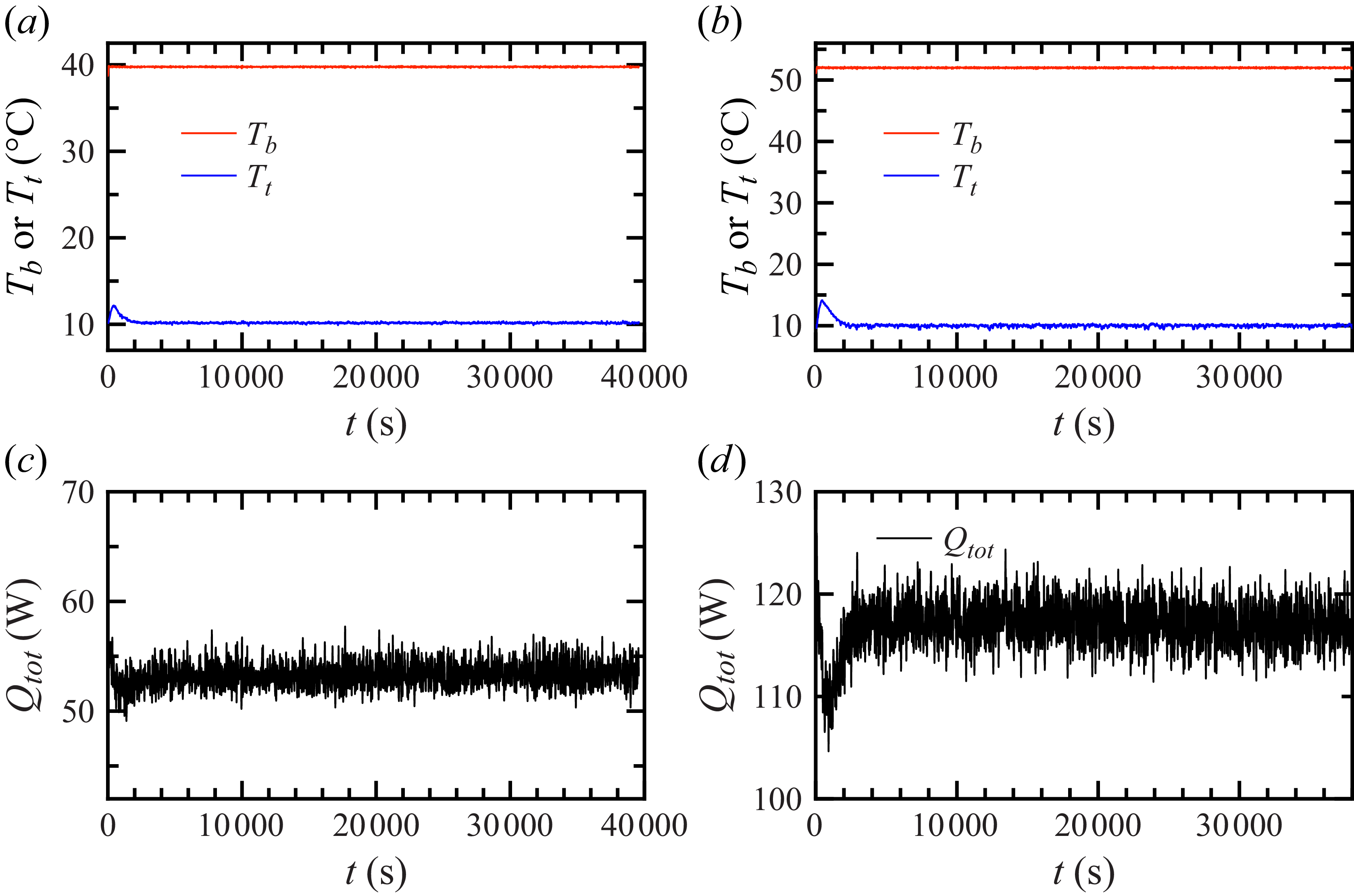
 Tb
 Tt
 Qtot
 ΔTsup=−2∘C
 ΔTsup=10∘C

 Tm
 Tb
 Pr
 Ra
 Nu=0.116Ra0.303±0.009
 Nu=0.1143Ra0.306
 Nur
 ΔTsup
 Nur=0.118×ΔTsup+1
 ∘C
 ∘C
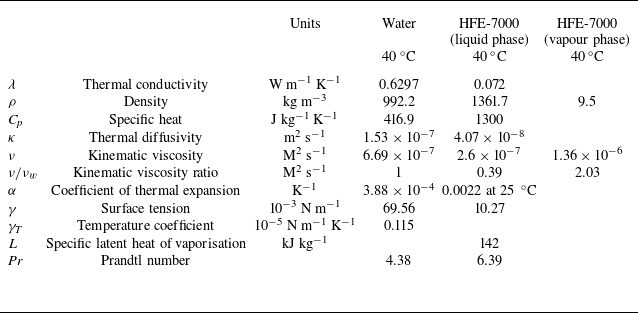

 ΔTsup=0∘C


 ΔTsup=2∘C

 z
 Zint=92
 ∘C

 ΔTsup
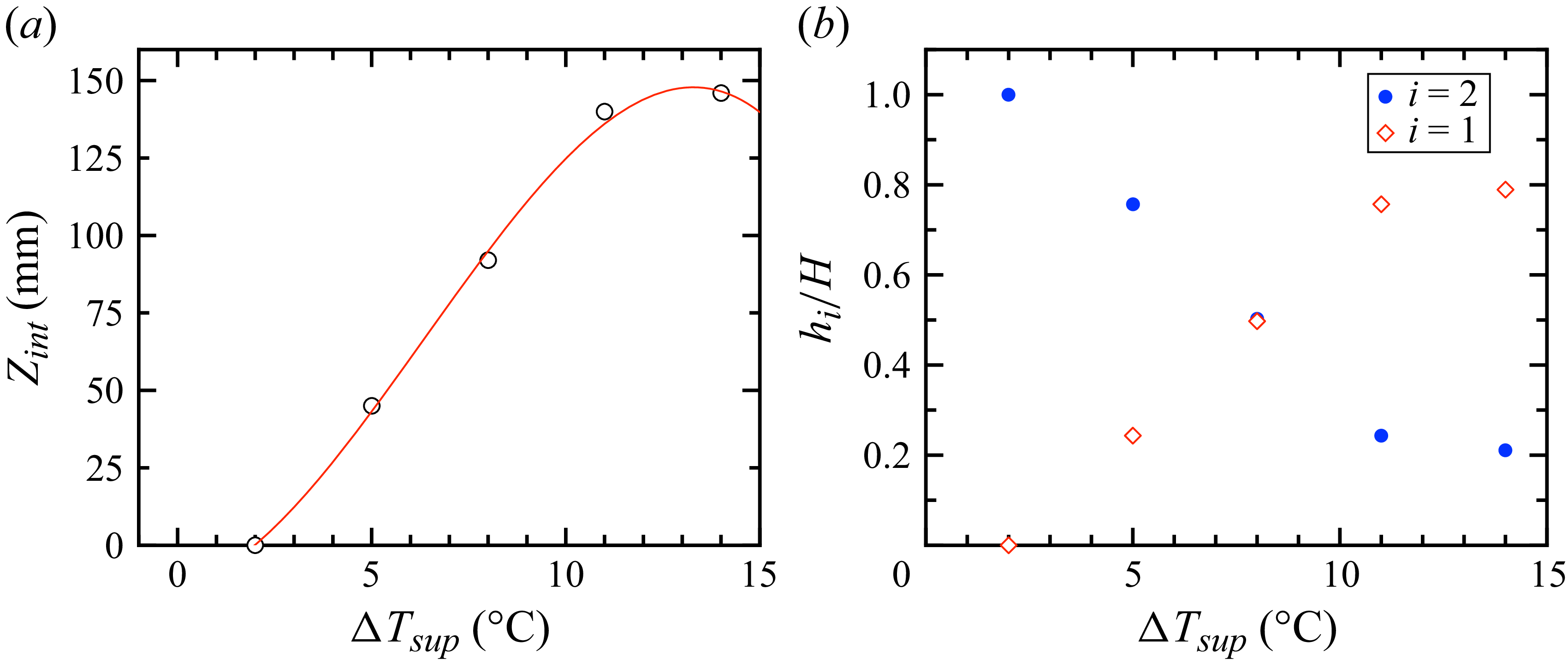
 Zint
 …
 hi/H

 ΔTsup
 Tn(z)≡(T(z)−Tt)/(Tb−Tt)
 Δbm≡T(H/4)−T(H/2)
 Δmt≡T(H/2)−T(3H/4)
 Δbm/Δ
 Δmt/Δ

 ∘C
 ∘C
 ∘C
 ΔTsup<0
 ΔTsup
 Tint−Tcr
 δTint
 δTint/Δ

 H/4
 H/2
 3H/4
 θ
 θk
 δk/⟨δk⟩
 ΔTsup=6∘C
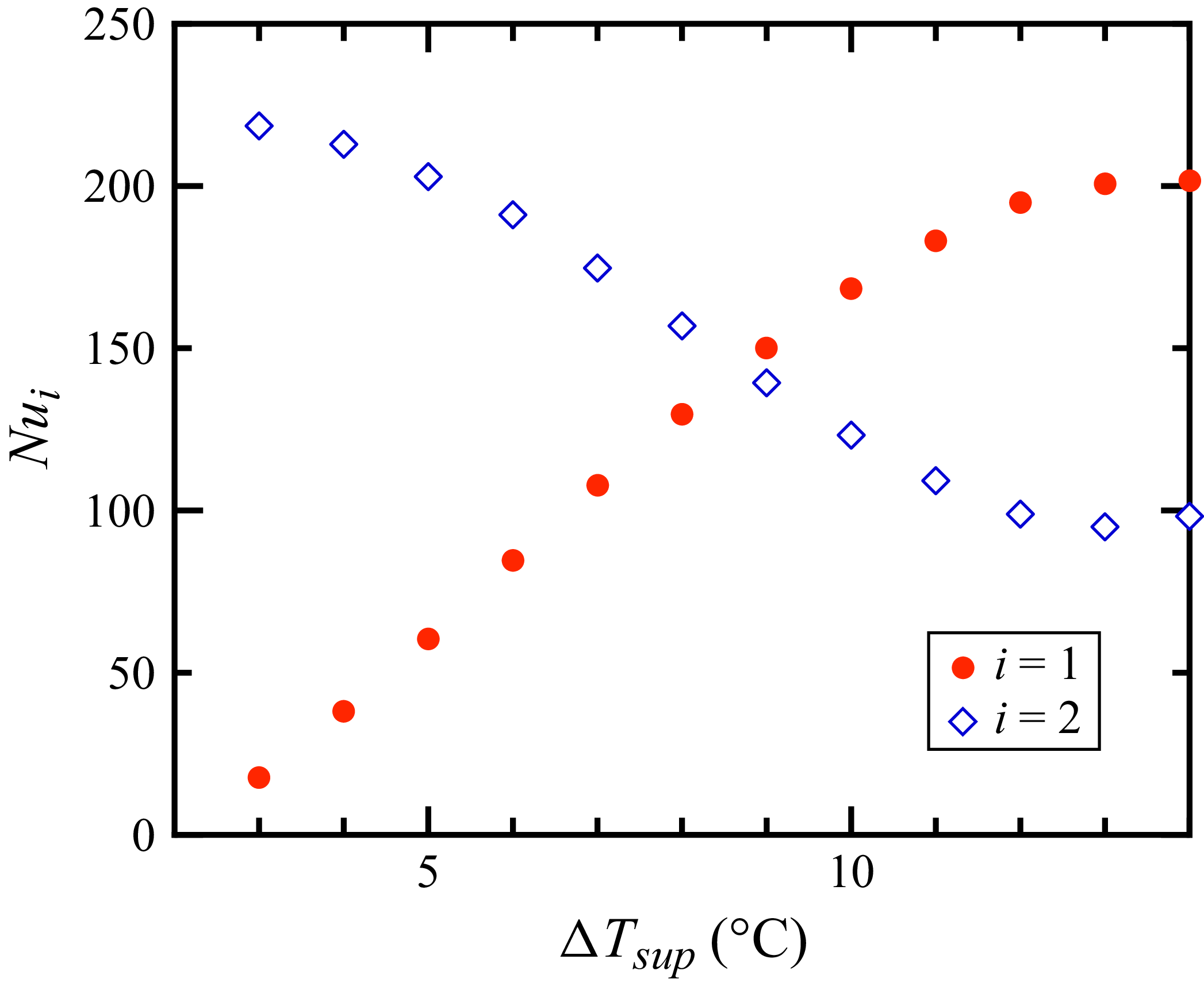
 i
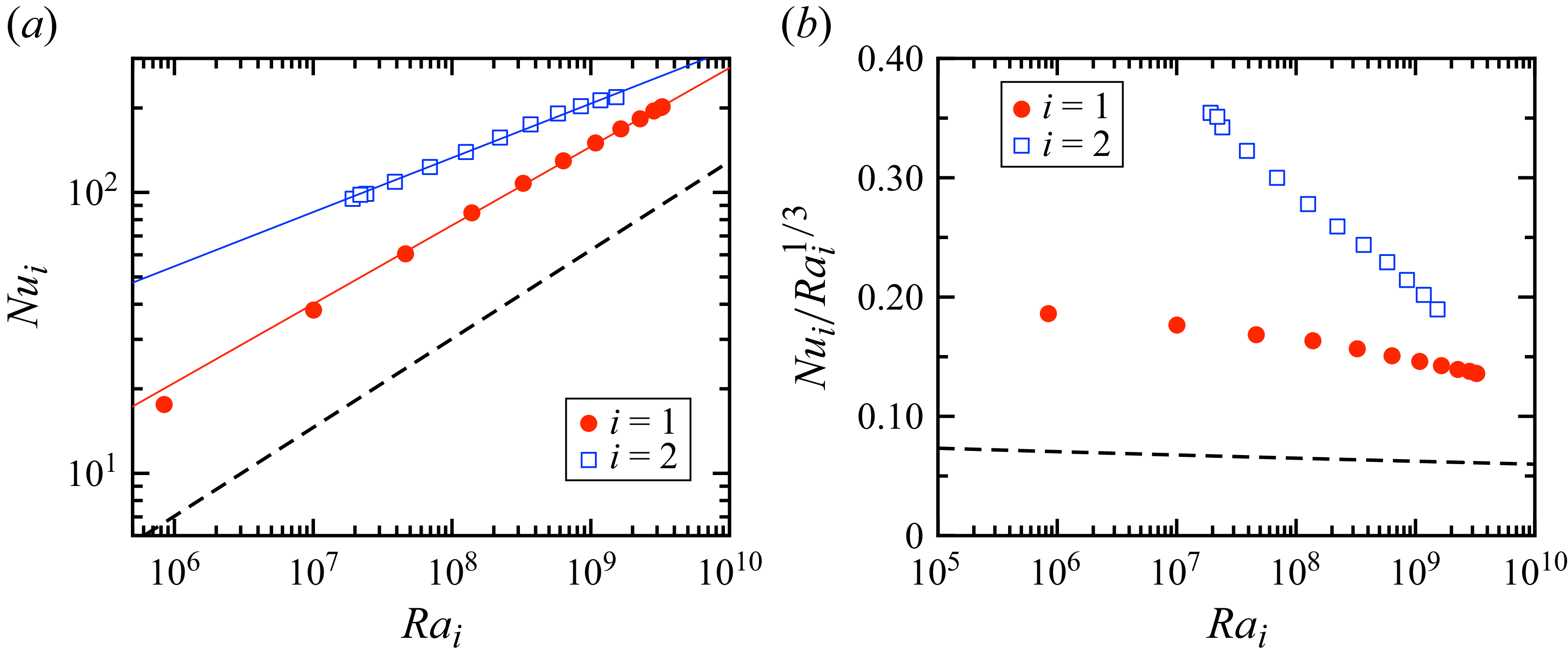
 i
 i
 Nu=0.0897Ra0.316
 Nu1=0.44Ra10.280±0.003
 Nu2=3.78Ra20.193±0.004
 Nui/Rai1/3
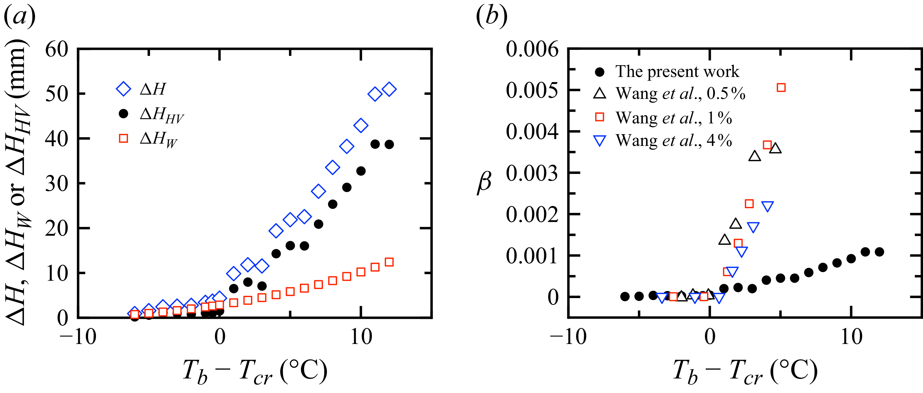
 ϕ=0.86%
 ϕ=0.5%
 ϕ=1%
 ϕ=4%