1 Introduction
Thermal convection of a Boussinesq fluid in a rotating sphere is a classical problem in fluid dynamics that has important implications for the heat transfer and generation of magnetic fields in astrophysical bodies. In the liquid core of planets, the Ekman number,
 $Ek$
, which measures the viscous effects compared with the Coriolis force, and the Rossby number,
 $Ro$
, which measures the nonlinear inertial effects compared with the Coriolis force, are very small, so convection is strongly influenced by the global rotation. The linear onset of thermal convection in a spherical geometry for
 $Ek\ll 1$
and
 $Ek/Pr\ll 1$
(where
 $Pr$
is the Prandtl number, the ratio of the kinematic viscosity to thermal diffusivity of the fluid) is now well understood following the theoretical work of Roberts (Reference Roberts1968), Busse (Reference Busse1970), Soward (Reference Soward1977), Yano (Reference Yano1992), Jones, Soward & Mussa (Reference Jones, Soward and Mussa2000), confirmed by experimental studies (Carrigan & Busse Reference Carrigan and Busse1983; Cordero & Busse Reference Cordero and Busse1992; Cardin & Olson Reference Cardin and Olson1994) and numerical models (Or & Busse Reference Or and Busse1987; Zhang Reference Zhang1992a
; Zhang & Jones Reference Zhang and Jones1993; Ardes, Busse & Wicht Reference Ardes, Busse and Wicht1997; Dormy et al.
Reference Dormy, Soward, Jones, Jault and Cardin2004). At the linear onset, the thermal instability takes the form of columnar flows aligned with the rotation axis, whose axial vorticity has much smaller variations along the rotation axis than in the azimuthal and cylindrical radial directions to accommodate the Proudman–Taylor theorem. These convective columns drift in the azimuthal direction, analogously to Rossby waves, and are therefore called thermal Rossby waves.
The properties of nonlinear convection for small
 $Ek$
and
 $Ro$
have received considerable attention but are still not fully understood (e.g. Jones (Reference Jones and Schubert2007), Aurnou et al. (Reference Aurnou, Calkins, Cheng, Julien, King, Nieves, Soderlund and Stellmach2015) for a review). At the onset of instability, any infinitesimal perturbation grows exponentially until nonlinear effects saturate the growing solution. If the transition from the basic conduction state to the convection state is continuous, then we have a supercritical branch of convection (e.g. Manneville Reference Manneville2004). However, in some classical problems of fluid dynamics, the nonlinearities can promote the instability rather than saturating it. This leads to a subcritical bifurcation, meaning that once the instability develops above the linear onset, it might continue to exist when the controlling parameter is decreased below the critical value for linear instability. Subcritical behaviour has been observed in various convective systems such as double-diffusive convection (e.g. Costa, Knobloch & Weiss Reference Costa, Knobloch and Weiss1981), planar convection with moderate rotation (Veronis Reference Veronis1966; Bajaj, Ahlers & Pesch Reference Bajaj, Ahlers and Pesch2002) and Bénard–Marangoni convection (e.g. Scanlon & Segel Reference Scanlon and Segel1967). In thermal convection in a rotating spherical geometry, weakly nonlinear analyses show that the nature of the bifurcation from the basic conduction state to the thermal Rossby waves might change from supercritical to subcritical in the limit of small Ekman numbers, at least in the case of internal heating (Soward Reference Soward1977; Plaut et al.
Reference Plaut, Lebranchu, Simitev and Busse2008). However, nonlinear numerical models, which can be computed down to
 $Ek=O(10^{-6})$
, always find that the bifurcation is supercritical (e.g. Zhang Reference Zhang1992a
; Aubert, Gillet & Cardin Reference Aubert, Gillet and Cardin2003; Grote & Busse Reference Grote and Busse2001; Christensen Reference Christensen2002; Morin & Dormy Reference Morin and Dormy2004; Yadav et al.
Reference Yadav, Gastine, Christensen, Duarte and Reiners2016). This possibly means that the numerical models are not run at sufficiently small Ekman numbers to properly capture the properties of nonlinear convection for planetary cores (where
 $Ek=O(10^{-15})$
), even near the onset of convection. Current numerical models might thus misrepresent realistic planetary convection for more vigorous thermal driving as well. The scaling laws for the global properties of convection that are derived from the numerical models (e.g. Christensen Reference Christensen2002) would then not be applicable for natural objects. Furthermore, calculations are generally performed for Prandtl numbers close to unity while liquid metals have smaller
 $Pr$
; for instance, the liquid iron in the Earth’s core is thought to have
 $Pr\approx 10^{-1}$
(Pozzo et al.
Reference Pozzo, Davies, Gubbins and Alfe2012). Subcriticality is observed for small Prandtl numbers in planar convection with moderate rotation (Veronis Reference Veronis1966; Clever & Busse Reference Clever and Busse2000), and the value of
 $Pr$
might be equally significant for the nature of the bifurcation at onset in rapidly rotating spherical convection.
The objective of the present paper is to describe nonlinear convection for
 $Ek\ll 1$
,
 $Ek/Pr\ll 1$
and
 $Ro\ll 1$
near the onset. In order to map the different hydrodynamical regimes, we carry out an extensive exploration of the parameter space. To alleviate part of the computational limitations that apply to global models of planetary cores, we use the quasi-geostrophic (QG) approximation that was developed by Busse & Or (Reference Busse and Or1986) for thermal convection in the annulus geometry of Busse (Reference Busse1970) with curved boundaries, and subsequently used and modified for the spherical geometry by Cardin & Olson (Reference Cardin and Olson1994), Aubert et al. (Reference Aubert, Gillet and Cardin2003), Morin & Dormy (Reference Morin and Dormy2004), Schaeffer & Cardin (Reference Schaeffer and Cardin2005), Gillet & Jones (Reference Gillet and Jones2006), Gillet et al. (Reference Gillet, Brito, Jault and Nataf2007), Plaut et al. (Reference Plaut, Lebranchu, Simitev and Busse2008), Calkins et al. (Reference Calkins, Aurnou, Eldredge and Julien2012). The model assumes that the flow is geostrophically balanced, i.e. the Coriolis force balances the pressure gradient at leading order. By neglecting the variation of the axial vorticity along the rotation axis, we can model the flow in two dimensions. This is an important limitation to the full dynamics of rotating convection, but this exploratory study aims to inform future three-dimensional studies. The QG approximation allows us to model thermal convection for Ekman numbers as low as
 $10^{-8}$
. Results from the numerical implementation of the QG approximation in a spherical geometry have been successfully benchmarked against the asymptotic theory (Gillet & Jones Reference Gillet and Jones2006; Labbé, Jault & Gillet Reference Labbé, Jault and Gillet2015) and three-dimensional (3-D) numerical models (Aubert et al.
Reference Aubert, Gillet and Cardin2003; Plaut et al.
Reference Plaut, Lebranchu, Simitev and Busse2008) for the onset of convection, and against laboratory experiments in rotating convection (Aubert et al.
Reference Aubert, Gillet and Cardin2003; Gillet et al.
Reference Gillet, Brito, Jault and Nataf2007) and in shear flows (Schaeffer & Cardin Reference Schaeffer and Cardin2005) for the nonlinear regime.
The main issue of the QG approximation for rotating spherical convection is that the basic temperature background has a spherical symmetry. Treating the temperature as a 2-D field is therefore an unjustified approximation, although it has been successfully used in previous studies when compared with results from 3-D models and laboratory experiments (Aubert et al.
Reference Aubert, Gillet and Cardin2003; Morin & Dormy Reference Morin and Dormy2004; Gillet et al.
Reference Gillet, Brito, Jault and Nataf2007; Plaut et al.
Reference Plaut, Lebranchu, Simitev and Busse2008). In the present study, we follow the work of Schaeffer & Cardin (Reference Schaeffer and Cardin2006) by coupling the 2-D velocity to a 3-D implementation of the temperature in the whole sphere. The coupling terms require interpolations from the 2-D and 3-D grids. The hybrid QG–3-D approach can therefore only be efficient, in term of the computational time, if the temperature is solved on a 3-D grid that is coarser than the 2-D grid used for the velocity. This is particularly appropriate to model fluids with small Prandtl numbers, where the dissipative scale of the temperature is larger than the viscous dissipation scale. Recent studies of rapidly rotating convection in small Prandtl number fluids have shown that the Prandtl number has a significant influence on the convection, especially on the dominant length and time scales of the flow (Gillet et al.
Reference Gillet, Brito, Jault and Nataf2007; Calkins et al.
Reference Calkins, Aurnou, Eldredge and Julien2012; King & Aurnou Reference King and Aurnou2013). In this paper, we vary
 $Pr$
between
 $[10^{-2},10^{-1}]$
. Note that for small Prandtl numbers, convection cells attached to the equator of the outer sphere are preferred to thermal Rossby waves at the linear onset of convection when the Ekman number is moderately small (Zhang & Busse Reference Zhang and Busse1987; Busse & Simitev Reference Busse and Simitev2004; Plaut & Busse Reference Plaut and Busse2005; Sánchez, Garcia & Net Reference Sánchez, Garcia and Net2016). In the limit
 $Ek\ll 1$
and
 $Ek/Pr\ll 1$
, the critical Rayleigh number at the onset of these equatorially attached modes scales as
 $Ek^{-2}$
, while the critical Rayleigh number at the onset of the thermal Rossby waves scales as
 $Ek^{-4/3}$
(Busse & Simitev Reference Busse and Simitev2004). The equatorially attached modes are therefore unlikely to occur in the Earth’s core. The 3-D numerical simulations of Ardes et al. (Reference Ardes, Busse and Wicht1997) show that the thermal Rossby waves are preferred for
 $Ek\leqslant 10^{-4}$
when
 $Pr=10^{-1}$
and
 $Ek\leqslant 10^{-6}$
when
 $Pr=10^{-2}$
. The equatorially attached modes are outside the scope of this paper, so we restrict our study to this range of small Ekman numbers.
For simplicity, we consider only thermal convection in a full sphere without a solid inner core to avoid the singularity of the QG approach at the tangent cylinder. Consequently, the thermal convection is driven by an homogenous internal heating, which is a well-studied variation of the classical problem of thermal convection in a rapidly rotating sphere (Jones et al. Reference Jones, Soward and Mussa2000), and is relevant for the early history of the Earth’s core (e.g. Olson Reference Olson2013).
The layout of the paper is as follows. First, we derive the formulation of the hybrid QG–3-D model that describes thermal convection in a rapidly rotating sphere in § 2. Then in § 3, we discuss the results from the nonlinear simulations carried out near the onset for small Ekman numbers. Subcritical convection, hysteresis and nonlinear oscillations are reported. A discussion of the results is given in § 4. In appendix A, the results at the linear onset of convection obtained with our hybrid model are compared with results from the asymptotic theory and from previous quasi-geostrophic and 3-D numerical models.
2 Formulation of the model
We study thermal Boussinesq convection in a rotating sphere driven by internal heating. The system rotates at a constant angular velocity
 $\unicode[STIX]{x1D6FA}\boldsymbol{e}_{z}$
. The acceleration due to gravity is radial and linear,
 $\boldsymbol{g}=g_{0}r\boldsymbol{e}_{r}$
. The radius of the sphere is
 $r_{o}$
and no inner core is present. The fluid has kinematic viscosity
 $\unicode[STIX]{x1D708}$
, thermal diffusivity
 $\unicode[STIX]{x1D705}$
, density
 $\unicode[STIX]{x1D70C}$
, heat capacity at constant pressure
 $C_{p}$
and thermal expansion coefficient
 $\unicode[STIX]{x1D6FC}$
, all of which are constant. We consider an homogeneous internal volumetric heating
 $S$
. In the absence of convection, the static temperature profile
 $T_{s}$
is calculated by solving the diffusive heat equation and can be written as
 $$\begin{eqnarray}\displaystyle T_{s}(r)=T_{o}+\frac{S}{6\unicode[STIX]{x1D705}\unicode[STIX]{x1D70C}C_{p}}(r_{o}^{2}-r^{2}), & & \displaystyle\end{eqnarray}$$
where
 $T_{o}$
is the imposed temperature at the boundary,
 $r=r_{o}$
. The governing equations are solved in dimensionless form, obtained by scaling lengths with
 $r_{o}$
, times with
 $r_{o}^{2}/\unicode[STIX]{x1D708}$
and temperature with
 $\unicode[STIX]{x1D708}Sr_{o}^{2}/(6\unicode[STIX]{x1D70C}C_{p}\unicode[STIX]{x1D705}^{2})$
. The system of dimensionless equations is:
 $$\begin{eqnarray}\displaystyle & \displaystyle \frac{\unicode[STIX]{x2202}\boldsymbol{u}}{\unicode[STIX]{x2202}t}+(\boldsymbol{u}\boldsymbol{\cdot }\unicode[STIX]{x1D735})\boldsymbol{u}+\frac{2}{Ek}\boldsymbol{e}_{z}\times \boldsymbol{u}=-\unicode[STIX]{x1D735}p+\unicode[STIX]{x1D6FB}^{2}\boldsymbol{u}+Ra\unicode[STIX]{x1D6E9}\boldsymbol{r}, & \displaystyle\end{eqnarray}$$
 $$\begin{eqnarray}\displaystyle & \displaystyle \unicode[STIX]{x1D735}\boldsymbol{\cdot }\boldsymbol{u}=0, & \displaystyle\end{eqnarray}$$
 $$\begin{eqnarray}\displaystyle & \displaystyle \frac{\unicode[STIX]{x2202}\unicode[STIX]{x1D6E9}}{\unicode[STIX]{x2202}t}+\boldsymbol{u}\boldsymbol{\cdot }\unicode[STIX]{x1D735}\unicode[STIX]{x1D6E9}-\frac{2}{Pr}ru_{r}=\frac{1}{Pr}\unicode[STIX]{x1D6FB}^{2}\unicode[STIX]{x1D6E9}, & \displaystyle\end{eqnarray}$$
 $\boldsymbol{u}$
is the velocity field,
 $p$
the modified pressure, which includes the centrifugal potential, and
 $\unicode[STIX]{x1D6E9}$
the temperature perturbation relative to the static temperature (2.1).
The dimensionless numbers are the Ekman number,
 $$\begin{eqnarray}\displaystyle Ek=\frac{\unicode[STIX]{x1D708}}{\unicode[STIX]{x1D6FA}r_{o}^{2}}, & & \displaystyle\end{eqnarray}$$
the Rayleigh number,
 $$\begin{eqnarray}\displaystyle Ra=\frac{\unicode[STIX]{x1D6FC}g_{0}Sr_{o}^{6}}{6\unicode[STIX]{x1D70C}C_{p}\unicode[STIX]{x1D708}\unicode[STIX]{x1D705}^{2}}, & & \displaystyle\end{eqnarray}$$
and the Prandtl number,
 $$\begin{eqnarray}\displaystyle Pr=\frac{\unicode[STIX]{x1D708}}{\unicode[STIX]{x1D705}}. & & \displaystyle\end{eqnarray}$$
At
 $r=r_{o}$
, the boundary condition for the velocity is no slip and impenetrable and the temperature is fixed,
 $$\begin{eqnarray}\displaystyle \boldsymbol{u}=\mathbf{0},\quad \unicode[STIX]{x1D6E9}=0\quad \text{at }r=r_{o}. & & \displaystyle\end{eqnarray}$$
We detail below the quasi-geostrophic formulation used to model the velocity field, the 3-D model used for temperature and the numerical method. Throughout this paper, we use both spherical coordinates
 $\boldsymbol{u}=(u_{r},u_{\unicode[STIX]{x1D703}},u_{\unicode[STIX]{x1D719}})$
and cylindrical polar coordinates
 $\boldsymbol{u}=(u_{s},u_{\unicode[STIX]{x1D719}},u_{z})$
.
2.1 Governing equation for the non-axisymmetric flow
We seek to model the system of equations (2.2)–(2.4) for small Ekman numbers. We choose the QG approximation to model the evolution of the velocity field (Or & Busse Reference Or and Busse1987; Brummell & Hart Reference Brummell and Hart1993; Cardin & Olson Reference Cardin and Olson1994; Plaut & Busse Reference Plaut and Busse2002; Aubert et al.
Reference Aubert, Gillet and Cardin2003; Jones, Rotvig & Abdulrahman Reference Jones, Rotvig and Abdulrahman2003; Morin & Dormy Reference Morin and Dormy2004; Schaeffer & Cardin Reference Schaeffer and Cardin2005; Gillet & Jones Reference Gillet and Jones2006; Calkins et al.
Reference Calkins, Aurnou, Eldredge and Julien2012; Teed, Jones & Hollerbach Reference Teed, Jones and Hollerbach2012). The QG approximation reduces the 3-D system to a 2-D system by taking advantage of the small variation of the flow along
 $z$
due to the rapid rotation (Gillet & Jones Reference Gillet and Jones2006). This approximation is only justified in the case of small slope of the boundaries, such as the Busse (Reference Busse1970) annulus. In the case of a sphere, the approximation is therefore not rigorously justified in any asymptotic limit. Consequently, the QG model is intended as a simplified model of convection in a rapidly rotating sphere that allows us to investigate unexplored regions of the parameter space. When possible, comparisons with theoretical, experimental and 3-D numerical models show that the QG model correctly reproduces key properties of the full system (Aubert et al.
Reference Aubert, Gillet and Cardin2003; Morin & Dormy Reference Morin and Dormy2004; Gillet & Jones Reference Gillet and Jones2006; Gillet et al.
Reference Gillet, Brito, Jault and Nataf2007; Plaut et al.
Reference Plaut, Lebranchu, Simitev and Busse2008).
The QG model assumes that the fluid dynamics is dominated by the geostrophic balance, i.e. the Coriolis force balances the pressure gradient. The geostrophic velocity
 $\boldsymbol{u}^{g}$
is invariant along
 $z$
and
 $\boldsymbol{u}^{g}=(u_{s}^{g},u_{\unicode[STIX]{x1D719}}^{g},0)$
in cylindrical polar coordinates. By taking the
 $z$
-component of the curl of the momentum equation (2.2) and averaging it along
 $z$
, we obtain the equation for the axial vorticity,
 $\unicode[STIX]{x1D701}^{g}=(\unicode[STIX]{x1D735}\times \boldsymbol{u}^{g})\boldsymbol{\cdot }\boldsymbol{e}_{z}$
,
 $$\begin{eqnarray}\displaystyle \frac{\unicode[STIX]{x2202}\unicode[STIX]{x1D701}^{g}}{\unicode[STIX]{x2202}t}+(\boldsymbol{u}^{g}\boldsymbol{\cdot }\unicode[STIX]{x1D735})\unicode[STIX]{x1D701}^{g}-\left(\frac{2}{Ek}+\unicode[STIX]{x1D701}^{g}\right)\left\langle \frac{\unicode[STIX]{x2202}u_{z}}{\unicode[STIX]{x2202}z}\right\rangle =\unicode[STIX]{x1D6FB}_{e}^{2}\unicode[STIX]{x1D701}^{g}-Ra\left\langle \frac{\unicode[STIX]{x2202}\unicode[STIX]{x1D6E9}}{\unicode[STIX]{x2202}\unicode[STIX]{x1D719}}\right\rangle , & & \displaystyle\end{eqnarray}$$
with
 $$\begin{eqnarray}\displaystyle \unicode[STIX]{x1D6FB}_{e}^{2}A\equiv \frac{1}{s}\frac{\unicode[STIX]{x2202}}{\unicode[STIX]{x2202}s}\left(s\frac{\unicode[STIX]{x2202}A}{\unicode[STIX]{x2202}s}\right)+\frac{1}{s^{2}}\frac{\unicode[STIX]{x2202}^{2}A}{\unicode[STIX]{x2202}\unicode[STIX]{x1D719}^{2}}, & & \displaystyle\end{eqnarray}$$
and
 $$\begin{eqnarray}\displaystyle \langle A\rangle \equiv \frac{1}{2H}\int _{-H}^{+H}A\,\text{d}z, & & \displaystyle\end{eqnarray}$$
where
 $H=\sqrt{1-s^{2}}$
is the axial distance from the spherical boundary to the equatorial plane.
The axial velocity
 $u_{z}$
is assumed to be linear in
 $z$
. Three-dimensional linear convection models with internal heating show that the variation in
 $z$
of
 $u_{z}$
is not exactly linear, but it is a reasonable assumption because the variations in
 $z$
with respect to the linear profile are small compared with the variations in
 $s$
and
 $\unicode[STIX]{x1D719}$
(Gillet & Jones Reference Gillet and Jones2006).
The velocity
 $\boldsymbol{u}^{g}$
can be described by a streamfunction
 $\unicode[STIX]{x1D713}$
that describes the non-axisymmetric (i.e.
 $\unicode[STIX]{x1D719}$
-dependent) geostrophic flow with the addition of an axisymmetric azimuthal flow,
 $$\begin{eqnarray}\displaystyle \boldsymbol{u}^{g}=\frac{1}{H}\unicode[STIX]{x1D735}\times (H\unicode[STIX]{x1D713}\boldsymbol{e}_{z})+\overline{u_{\unicode[STIX]{x1D719}}^{g}}\boldsymbol{e}_{\unicode[STIX]{x1D719}}, & & \displaystyle\end{eqnarray}$$
where
 $$\begin{eqnarray}\displaystyle \overline{A}\equiv \frac{1}{2\unicode[STIX]{x03C0}}\int _{0}^{2\unicode[STIX]{x03C0}}A\,\text{d}\unicode[STIX]{x1D719}. & & \displaystyle\end{eqnarray}$$
This choice for the streamfunction implies that the divergence of
 $\boldsymbol{u}^{g}$
in the equatorial plane is non-zero because of the return axial flow due to the slope of the boundaries,
 $$\begin{eqnarray}\displaystyle \unicode[STIX]{x1D735}_{e}\boldsymbol{\cdot }\boldsymbol{u}^{g}=-\unicode[STIX]{x1D6FD}u_{s}^{g}, & & \displaystyle\end{eqnarray}$$
where
 $$\begin{eqnarray}\displaystyle \unicode[STIX]{x1D735}_{e}\boldsymbol{\cdot }\boldsymbol{A}\equiv \frac{1}{s}\frac{\unicode[STIX]{x2202}sA_{s}}{\unicode[STIX]{x2202}s}+\frac{1}{s}\frac{\unicode[STIX]{x2202}A_{\unicode[STIX]{x1D719}}}{\unicode[STIX]{x2202}\unicode[STIX]{x1D719}}, & & \displaystyle\end{eqnarray}$$
and
 $$\begin{eqnarray}\displaystyle \unicode[STIX]{x1D6FD}=\frac{1}{H}\frac{\text{d}H}{\text{d}s}=-\frac{s}{H^{2}}. & & \displaystyle\end{eqnarray}$$
The third term on the left-hand side of (2.9) requires us to determine
 $u_{z}$
at the boundary
 $z=\pm H$
:
 $$\begin{eqnarray}\displaystyle u_{z}|_{\pm H}=\pm \frac{1}{H}\boldsymbol{u}\boldsymbol{\cdot }\boldsymbol{n}|_{\pm H}\pm \unicode[STIX]{x1D6FD}Hu_{s}^{g}, & & \displaystyle\end{eqnarray}$$
where the normal vector at the boundary is
 $\boldsymbol{n}=\boldsymbol{e}_{r}$
. The normal component,
 $\boldsymbol{u}\boldsymbol{\cdot }\boldsymbol{n}|_{\pm H}$
, is the Ekman pumping induced by the viscous boundary layer and is determined by asymptotic methods (Greenspan Reference Greenspan1968),
 $$\begin{eqnarray}\displaystyle \boldsymbol{u}\boldsymbol{\cdot }\boldsymbol{n}|_{z=\pm H}=-\frac{Ek^{1/2}}{2}\boldsymbol{n}\boldsymbol{\cdot }\unicode[STIX]{x1D735}\times \left(\frac{\boldsymbol{n}\times \boldsymbol{u}\pm \boldsymbol{u}}{\sqrt{|\boldsymbol{n}\boldsymbol{\cdot }\boldsymbol{ e}_{\boldsymbol{z}}|}}\right)=Ek^{1/2}P(s,u_{s}^{g},u_{\unicode[STIX]{x1D719}}^{g}). & & \displaystyle\end{eqnarray}$$
This analytical formulation is valid for a linear Ekman layer and for variations of the velocity that are slower than the rotation period and on larger length scales than
 $\mathit{O}(Ek^{1/2})$
. The function
 $P$
is derived for a spherical boundary in Schaeffer & Cardin (Reference Schaeffer and Cardin2005).
Our numerical code solves the equation for the evolution of the non-axisymmetric streamfunction
 $$\begin{eqnarray}\displaystyle \frac{\unicode[STIX]{x2202}}{\unicode[STIX]{x2202}t}{\mathcal{L}}\unicode[STIX]{x1D713}+(\boldsymbol{u}^{g}\boldsymbol{\cdot }\unicode[STIX]{x1D735}_{e}){\mathcal{L}}\unicode[STIX]{x1D713}-\left(\frac{2}{Ek}+{\mathcal{L}}\unicode[STIX]{x1D713}\right)\left(\frac{Ek^{1/2}P}{2H^{2}}+\unicode[STIX]{x1D6FD}u_{s}^{g}\right)=\unicode[STIX]{x1D6FB}_{e}^{2}{\mathcal{L}}\unicode[STIX]{x1D713}-Ra\left\langle \frac{\unicode[STIX]{x2202}\unicode[STIX]{x1D6E9}}{\unicode[STIX]{x2202}\unicode[STIX]{x1D719}}\right\rangle ,\qquad & & \displaystyle\end{eqnarray}$$
where
 $$\begin{eqnarray}\displaystyle {\mathcal{L}}\unicode[STIX]{x1D713}=\unicode[STIX]{x1D701}^{g}=-\unicode[STIX]{x1D6FB}_{e}^{2}\unicode[STIX]{x1D713}+\frac{1}{s}\frac{\unicode[STIX]{x2202}}{\unicode[STIX]{x2202}s}\left(\frac{s^{2}\unicode[STIX]{x1D713}}{H^{2}}\right). & & \displaystyle\end{eqnarray}$$
The no-slip and impenetrable boundary conditions imply that
 $$\begin{eqnarray}\displaystyle \unicode[STIX]{x1D713}=\frac{\unicode[STIX]{x2202}\unicode[STIX]{x1D713}}{\unicode[STIX]{x2202}s}=0\quad \text{at }s=1. & & \displaystyle\end{eqnarray}$$
At the centre of the sphere, the solution must be regular. Using a decomposition in Fourier modes,
 $$\begin{eqnarray}\displaystyle \unicode[STIX]{x1D713}(s,\unicode[STIX]{x1D719},t)=\mathop{\sum }_{m=1}^{+\infty }\hat{\unicode[STIX]{x1D713}}^{m}(s,t)\text{e}^{\text{i}m\unicode[STIX]{x1D719}}, & & \displaystyle\end{eqnarray}$$
the regularity condition is
 $$\begin{eqnarray}\displaystyle \hat{\unicode[STIX]{x1D713}}^{m}=O(s^{m})\quad \text{at }s=0. & & \displaystyle\end{eqnarray}$$
2.2 Governing equation for the zonal flow
In our model, the streamfunction
 $\unicode[STIX]{x1D713}$
only describes the non-axisymmetric motions, so the axisymmetric azimuthal flows, or zonal flows, are treated separately. We take the
 $\unicode[STIX]{x1D719}$
- and
 $z$
-averages of the
 $\unicode[STIX]{x1D719}$
-component of the momentum equation to obtain
 $$\begin{eqnarray}\displaystyle \frac{\unicode[STIX]{x2202}\overline{u_{\unicode[STIX]{x1D719}}^{g}}}{\unicode[STIX]{x2202}t}+\overline{u_{s}^{g}\frac{\unicode[STIX]{x2202}u_{\unicode[STIX]{x1D719}}^{g}}{\unicode[STIX]{x2202}s}}+\overline{\frac{u_{s}^{g}u_{\unicode[STIX]{x1D719}}^{g}}{s}}+\frac{2}{Ek}\langle \overline{u_{s}}\rangle =\unicode[STIX]{x1D6FB}^{2}\overline{u_{\unicode[STIX]{x1D719}}^{g}}-\frac{\overline{u_{\unicode[STIX]{x1D719}}^{g}}}{s^{2}}. & & \displaystyle\end{eqnarray}$$
Note that the geostrophic balance imposes that
 $\overline{u_{s}^{g}}=0$
. The fourth term on the left-hand side of (2.24) involves the
 $z$
-dependent radial velocity, which corresponds to the Ekman pumping term. Using the incompressibility of the fluid, it can be shown (Aubert et al.
Reference Aubert, Gillet and Cardin2003) that
 $$\begin{eqnarray}\displaystyle \langle \overline{u_{s}}\rangle =\frac{Ek^{1/2}}{2H^{3/2}}\overline{u_{\unicode[STIX]{x1D719}}^{g}}. & & \displaystyle\end{eqnarray}$$
The no-slip boundary condition at the outer sphere implies
 $$\begin{eqnarray}\displaystyle \overline{u_{\unicode[STIX]{x1D719}}^{g}}=0\quad \text{at }s=1. & & \displaystyle\end{eqnarray}$$
By symmetry at the centre,
 $$\begin{eqnarray}\displaystyle \overline{u_{\unicode[STIX]{x1D719}}^{g}}=0\quad \text{at }s=0. & & \displaystyle\end{eqnarray}$$
2.3 Governing equation for the temperature
The dimensionless equation for the evolution of the temperature perturbation in three dimensions is
 $$\begin{eqnarray}\displaystyle \frac{\unicode[STIX]{x2202}\unicode[STIX]{x1D6E9}}{\unicode[STIX]{x2202}t}+\boldsymbol{u}^{3d}\boldsymbol{\cdot }\unicode[STIX]{x1D735}\unicode[STIX]{x1D6E9}=\frac{1}{Pr}(2ru_{r}^{3d}+\unicode[STIX]{x1D6FB}^{2}\unicode[STIX]{x1D6E9}), & & \displaystyle\end{eqnarray}$$
where
 $\boldsymbol{u}^{3d}$
is the velocity in three dimensions. In cylindrical polar coordinates,
 $$\begin{eqnarray}\displaystyle \boldsymbol{u}^{3d}=(u_{s}^{g},u_{\unicode[STIX]{x1D719}}^{g},Ek^{1/2}zP+\unicode[STIX]{x1D6FD}zu_{s}^{g}). & & \displaystyle\end{eqnarray}$$
The temperature is fixed at the outer boundary so
 $$\begin{eqnarray}\displaystyle \unicode[STIX]{x1D6E9}=0\quad \text{at }r=1. & & \displaystyle\end{eqnarray}$$
At the centre, the heat flux of the spherically averaged temperature perturbation is zero,
 $$\begin{eqnarray}\displaystyle \left\langle \frac{\unicode[STIX]{x2202}\unicode[STIX]{x1D6E9}}{\unicode[STIX]{x2202}r}\right\rangle _{{\mathcal{S}}}=\int _{{\mathcal{S}}}\frac{\unicode[STIX]{x2202}\unicode[STIX]{x1D6E9}}{\unicode[STIX]{x2202}r}\,\text{d}{\mathcal{S}}=0\quad \text{at }r=0, & & \displaystyle\end{eqnarray}$$
where
 ${\mathcal{S}}$
is a spherical surface. By symmetry, the non-spherically symmetric components of
 $\unicode[STIX]{x1D6E9}$
are zero,
 $$\begin{eqnarray}\displaystyle \unicode[STIX]{x1D6E9}-\langle \unicode[STIX]{x1D6E9}\rangle _{{\mathcal{S}}}=0\quad \text{at }r=0. & & \displaystyle\end{eqnarray}$$
2.4 Numerical method
In summary, the governing equations of our hybrid QG–3-D model are
 $$\begin{eqnarray}\displaystyle & \displaystyle \frac{\unicode[STIX]{x2202}}{\unicode[STIX]{x2202}t}{\mathcal{L}}\unicode[STIX]{x1D713}+(\boldsymbol{u}\boldsymbol{\cdot }\unicode[STIX]{x1D735}_{e}){\mathcal{L}}\unicode[STIX]{x1D713}-\left(\frac{2}{Ek}+{\mathcal{L}}\unicode[STIX]{x1D713}\right)\left(\frac{Ek^{1/2}P}{2H^{2}}+\unicode[STIX]{x1D6FD}u_{s}\right)=\unicode[STIX]{x1D6FB}_{e}^{2}{\mathcal{L}}\unicode[STIX]{x1D713}-Ra\left\langle \frac{\unicode[STIX]{x2202}\unicode[STIX]{x1D6E9}}{\unicode[STIX]{x2202}\unicode[STIX]{x1D719}}\right\rangle ,\qquad & \displaystyle\end{eqnarray}$$
 $$\begin{eqnarray}\displaystyle & \displaystyle \frac{\unicode[STIX]{x2202}\overline{u_{\unicode[STIX]{x1D719}}}}{\unicode[STIX]{x2202}t}+\overline{u_{s}\frac{\unicode[STIX]{x2202}u_{\unicode[STIX]{x1D719}}}{\unicode[STIX]{x2202}s}}+\overline{\frac{u_{s}u_{\unicode[STIX]{x1D719}}}{s}}+\frac{\overline{u_{\unicode[STIX]{x1D719}}}}{Ek^{1/2}H^{3/2}}=\unicode[STIX]{x1D6FB}^{2}\overline{u_{\unicode[STIX]{x1D719}}}-\frac{\overline{u_{\unicode[STIX]{x1D719}}}}{s^{2}}, & \displaystyle\end{eqnarray}$$
 $$\begin{eqnarray}\displaystyle & \displaystyle \frac{\unicode[STIX]{x2202}\unicode[STIX]{x1D6E9}}{\unicode[STIX]{x2202}t}+\boldsymbol{u}^{3d}\boldsymbol{\cdot }\unicode[STIX]{x1D735}\unicode[STIX]{x1D6E9}=\frac{1}{Pr}(2ru_{r}^{3d}+\unicode[STIX]{x1D6FB}^{2}\unicode[STIX]{x1D6E9}), & \displaystyle\end{eqnarray}$$
 $g$
have been removed for clarity.
Equations (2.33) and (2.34) are solved on a 2-D grid in the equatorial plane. A second-order finite difference scheme is implemented in radius with irregular spacing (finer near the outer boundary). In the azimuthal direction, the streamfunction and zonal velocity are expanded in Fourier modes. Equation (2.35) is solved on a 3-D grid. Similarly to the 2-D grid, a finite difference scheme is used in radius. The temperature is expanded in spherical harmonics
 $Y_{l}^{m}$
in the angular coordinates with
 $l$
representing the latitudinal degree and
 $m$
the azimuthal mode. This allows for a simple implementation of the boundary conditions at the centre. A Crank–Nicolson scheme is implemented for the time integration of the diffusion terms and an Adams–Bashforth procedure is used for the other terms. Our hybrid approach is numerically efficient compared with a fully 3-D approach when considering small Prandtl numbers, i.e. when the diffusion of the temperature happens on shorter time scales than the viscous dissipation. In this case, the 3-D grid of the temperature requires less radial points and azimuthal modes than the 2-D grid of the velocity, so smaller grid steps and time step can be used for the velocity. The most demanding nonlinear simulations were run at
 $Ek=10^{-8}$
. The numerical resolution required to resolve the simulation run at
 $Ek=10^{-8}$
and
 $Pr=10^{-1}$
for the largest Rayleigh number (
 $Ra\approx 6Ra_{c}$
) is
 $1600$
radial points,
 $300$
Fourier modes
 $m$
for the 2-D velocity grid and
 $800$
radial points,
 $200$
degrees
 $l$
and
 $200$
modes
 $m$
of the spherical harmonics for the 3-D temperature grid.
The buoyancy term in (2.33) requires the integration of the temperature along
 $z$
for each point of coordinates
 $(s,\unicode[STIX]{x1D719})$
on the 2-D grid at each time step. To do so, we use a linear interpolation in
 $r$
and
 $\unicode[STIX]{x1D703}$
from the 3-D spherical grid onto a 3-D cylindrical projection of the velocity grid. The spectral decomposition in
 $\unicode[STIX]{x1D719}$
for the velocity and temperature allows a straightforward interpolation in spectral space. To calculate the 3-D velocity used for the advection of temperature, we use a linear interpolation in
 $s$
. Again, the interpolation in
 $\unicode[STIX]{x1D719}$
is straightforward in spectral space.
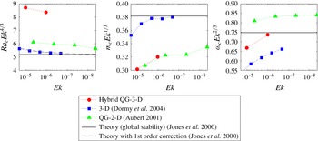
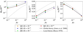
In order to benchmark the numerical model, we performed calculations with the linearised version of the code to determine the critical parameters at the linear onset of convection. The linear results are given in appendix A and compared with results from the asymptotic theory and from published numerical studies using either a 3-D or a QG model. The comparison shows that our numerical results tend to the asymptotic values as the Ekman number decreases. In the following, the critical Rayleigh number at the linear onset of convection calculated with our numerical code is denoted
 $Ra_{c}$
.
2.5 Definition of the output parameters
To quantify the global properties of convection, we use the following quantities calculated from the output of the simulations. In our dimensionless units, the Reynolds number corresponds to the root mean square (r.m.s.) value of the velocity,
 $$\begin{eqnarray}\displaystyle Re^{\ast }(t)=\left(\frac{3}{4\unicode[STIX]{x03C0}}\int _{0}^{2\unicode[STIX]{x03C0}}\int _{0}^{1}(u_{s}^{2}(s,\unicode[STIX]{x1D719},t)+u_{\unicode[STIX]{x1D719}}^{2}(s,\unicode[STIX]{x1D719},t))2H(s)s\,\text{d}s\,\text{d}\unicode[STIX]{x1D719}\right)^{1/2}, & & \displaystyle\end{eqnarray}$$
and
 $$\begin{eqnarray}\displaystyle Re=\frac{1}{\unicode[STIX]{x0394}t}\int _{\unicode[STIX]{x0394}t}Re^{\ast }(t)\,\text{d}t, & & \displaystyle\end{eqnarray}$$
where
 $u_{\unicode[STIX]{x1D719}}$
includes the zonal velocity. We measure the convective Reynolds number,
 $Re_{c}^{\ast }$
, as in (2.36) but including only the non-axisymmetric velocity. Its time average is denoted
 $Re_{c}$
. Similarly, we measure the zonal Reynolds number,
 $Re_{0}^{\ast }$
, including only the axisymmetric velocity, and its time average is denoted
 $Re_{0}$
. The time averages are calculated over a long period of time after the system reaches a statistical equilibrium.
We define the radial profile of the time-averaged zonal velocity as
 $$\begin{eqnarray}\displaystyle U_{0}(s)=\frac{1}{\unicode[STIX]{x0394}t}\int _{\unicode[STIX]{x0394}t}\overline{u_{\unicode[STIX]{x1D719}}}(s,t)\,\text{d}t, & & \displaystyle\end{eqnarray}$$
and the radial profile of the r.m.s. radial velocity,
 $$\begin{eqnarray}\displaystyle U_{s}(s)=\frac{1}{\unicode[STIX]{x0394}t}\int _{\unicode[STIX]{x0394}t}\left(\frac{1}{2\unicode[STIX]{x03C0}s}\int _{0}^{2\unicode[STIX]{x03C0}}u_{s}^{2}(s,\unicode[STIX]{x1D719},t)s\,\text{d}\unicode[STIX]{x1D719}\right)^{1/2}\,\text{d}t. & & \displaystyle\end{eqnarray}$$
The Nusselt number, which is the ratio of the total heat flux,
 $Q_{t}$
, to the conductive heat flux
 $Q_{\unicode[STIX]{x1D705}}$
, is often used to measure the efficiency of the convective heat transport. In a convective system with internal heating and fixed temperature boundaries, the mean total outward heat flux must balance heat production, so
 $Q_{t}=r_{o}S/3$
. To estimate the heat flux that is conducted along the spherically averaged temperature gradient, we define the equivalent internal heating,
 $S_{eq}$
, that would correspond to the purely conductive state with a temperature at the centre
 $T_{c}=T_{s}(r=0)+\langle \unicode[STIX]{x1D6E9}(r=0)\rangle _{{\mathcal{S}}}$
, where
 $\langle \unicode[STIX]{x1D6E9}(r=0)\rangle _{{\mathcal{S}}}$
is an output of the simulation. Assuming that
 $Q_{\unicode[STIX]{x1D705}}=r_{o}S_{eq}/3$
, we can define the Nusselt number,
 $Nu$
, as
 $$\begin{eqnarray}\displaystyle Nu=\frac{Q_{t}}{Q_{\unicode[STIX]{x1D705}}}=\frac{S}{S_{eq}}=\frac{1}{PrT_{c}}, & & \displaystyle\end{eqnarray}$$
where
 $S_{eq}=PrT_{c}S$
and
 $T_{c}=Pr^{-1}+\langle \unicode[STIX]{x1D6E9}(r=0)\rangle _{{\mathcal{S}}}$
. The decrease of the temperature at the centre due to convection is thus a good measure of the efficiency of the convective heat transport (Goluskin Reference Goluskin2016). We find that longer time integrations are required to ensure the saturation of
 $Nu$
than for the saturation of the kinetic energy.
We also measure the r.m.s. value of the axisymmetric temperature perturbation as
 $$\begin{eqnarray}\displaystyle \unicode[STIX]{x1D6E9}_{0}^{\ast }(t)=\left(\frac{3}{2}\int _{0}^{1}\int _{0}^{\unicode[STIX]{x03C0}}\overline{\unicode[STIX]{x1D6E9}}^{2}r^{2}\sin \unicode[STIX]{x1D703}\,\text{d}r\,\text{d}\unicode[STIX]{x1D703}\right)^{1/2}. & & \displaystyle\end{eqnarray}$$
3 Nonlinear calculations near the onset of convection
The data set presented in this paper contains approximately 120 simulations performed at small Ekman numbers,
 $Ek\in [10^{-8},10^{-5}]$
, and small Prandtl numbers,
 $Pr\in [10^{-2},10^{-1}]$
. The focus of the study is convection near the onset, so the Rayleigh number has been varied up to 10 times above the critical value at the onset of convection. The values of the critical Rayleigh number at the linear onset,
 $Ra_{c}$
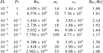
, are given in table 2 in appendix A for different
 $Ek$
and
 $Pr$
.
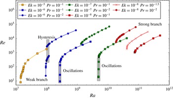
Time-averaged values of the Reynolds number,
 $Re$
, as a function of the Rayleigh number for different
 $Ek$
(identified by different colours) and
 $Pr$
(different symbols). The annotations correspond to the different regimes discussed in § 3.

To give an overview of the simulations and the results, figure 1 shows the Reynolds number,
 $Re$
, as a function of the Rayleigh number for the different Ekman numbers (identified by different colours) and Prandtl numbers (different symbols).
 $Re$
reaches values up to
 $10^{5}$
for the lowest Ekman and Prandtl numbers. Note that the local Rossby number, defined as the rotation period to the convective turnover time, is smaller than unity at all length scales in all of our simulations, in accordance with our approximation that the vortices are columnar at all scales (e.g. Nataf & Schaeffer Reference Nataf, Schaeffer and Schubert2015). At moderate Ekman numbers (
 $Ek=10^{-5}$
), we recover results previously described in the literature, such as the sequence of bifurcations between quasi-steady and time-dependent convection. This is discussed in § 3.1. In § 3.2, we describe a novel branch of convection and the occurrence of subcritical convection at low
 $Ek$
(
 $Ek=10^{-8}$
). The bridge between previous results at
 $Ek=10^{-5}$
and the new hydrodynamical regime at lower Ekman numbers is made at intermediate Ekman numbers (
 $Ek=10^{-7}-10^{-6}$
), where we observe interesting behaviours: a hysteresis loop (described in § 3.3) and nonlinear oscillations (§ 3.4). These different behaviours are annotated in figure 1.
3.1 Supercritical convection for
 $Ek=10^{-5}$

We begin our study with simulations performed at
 $Ek=10^{-5}$
and
 $Pr=10^{-1}$
in order to link the results obtained with our hybrid QG–3-D model to previous studies using either 3-D or QG models.
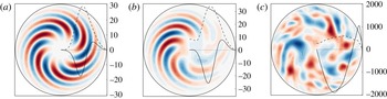
Snapshots of the streamfunction for
 $Ek=10^{-5}$
and
 $Pr=10^{-1}$
for (a)
 $Ra=1.13Ra_{c}$
, (b)
 $Ra=1.19Ra_{c}$
and (c)
 $Ra=7.06Ra_{c}$
. The time-averaged radial profiles of the zonal velocity,
 $U_{0}$
(solid line), and the r.m.s. radial velocity,
 $U_{s}$
(dashed line), are plotted according to the axis on the right-hand side.

For this Ekman number, the bifurcation from the basic conduction state is supercritical at
 $Ra=Ra_{c}$
. For values of
 $Ra$
just above
 $Ra_{c}$
, the convective flow consists of a thermal Rossby wave, a well-known flow pattern in rotating convection (e.g. Busse Reference Busse1970). Figure 2(a) shows a snapshot of the streamfunction (colour) for
 $Ra=1.13Ra_{c}$
. The linear thermal Rossby wave develops around the radius
 $s\approx 0.5$
and propagates eastward. For small Prandtl numbers, the thermal Rossby wave has a large tilt in the equatorial cross-section (Zhang Reference Zhang1992a
).
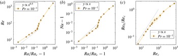
Evolution of the global properties of convection for
 $Ek=10^{-5}$
and
 $Pr=10^{-1}$
. The vertical and horizontal error bars represent the standard deviation in the time series.

Figure 3(a) shows the evolution of
 $Re$
as a function of the normalised Rayleigh number,
 $Ra/Ra_{c}-1$
. For
 $Ra/Ra_{c}<1.2$
, the evolution of
 $Re$
with
 $Ra/Ra_{c}-1$
can be approximated by a power law
 $Re\sim (Ra/Ra_{c}-1)^{0.42}$
. A sudden transition occurs at
 $Ra/Ra_{c}=1.2$
, after which the slope of the curve becomes steeper. Around this transition, or kink, the convection changes from quasi-steady to time dependent. The sequence of bifurcations that follows the kink has been previously documented in both 3-D models (Zhang Reference Zhang1992a
; Sun, Schubert & Glatzmaier Reference Sun, Schubert and Glatzmaier1993; Tilgner & Busse Reference Tilgner and Busse1997; Grote & Busse Reference Grote and Busse2001; Simitev & Busse Reference Simitev and Busse2003) and QG models (Schnaubelt & Busse Reference Schnaubelt and Busse1992; Morin & Dormy Reference Morin and Dormy2004). Our hybrid QG model reproduces this sequence: periodic vacillations (
 $Ra=1.18Ra_{c}$
), chaotic fluctuations with a localisation of the convection (
 $Ra=1.19Ra_{c}$
, figure 2
b) and bursts of convection (
 $Ra=1.21Ra_{c}$
). These various states are attributed to the interactions of the zonal flow and the axisymmetric temperature with the convective columns (Teed et al.
Reference Teed, Jones and Hollerbach2012). Interestingly, Morin & Dormy (Reference Morin and Dormy2004) find that the kink occurs closer to the onset of convection as the Ekman number decreases, implying that quasi-steady convection in the form of thermal Rossby waves is expected to occur within a vanishingly small range of Rayleigh numbers for
 $Ek\rightarrow 0$
. For higher Rayleigh number, the time dependence of the convection becomes irregular. Figure 2(c) shows the streamfunction for
 $Ra=7.06Ra_{c}$
. The thermal Rossby wave is no longer visible and the velocity comprises a wide range of length scales.
The kink at
 $Ra=1.2Ra_{c}$
is also clearly visible in the plot of
 $Nu$
as a function of
 $Ra/Ra_{c}-1$
shown in figure 3(b). Near the onset, Busse & Or (Reference Busse and Or1986) predicted that the evolution of the convective heat transport with the Rayleigh number follows a power law
 $Nu\sim Ra/Ra_{c}-1$
, which has later been confirmed by Gillet & Jones (Reference Gillet and Jones2006) with numerical results for
 $Pr>1$
. For
 $Ra<1.2Ra_{c}$
, our numerical results can be approximated by a power law of weaker exponent,
 $0.88$
. The slow increase of
 $Nu$
with the Rayleigh number for
 $Pr<1$
was previously observed by Gillet & Jones (Reference Gillet and Jones2006). After the kink, we have too few numerical points to determine whether the points still follow a power law.
In figure 2(a), we plot the time-averaged radial profile of the zonal velocity,
 $U_{0}$
, for
 $Ra=1.13Ra_{c}$
. Zonal flows are produced from the nonlinear interactions of the non-axisymmetric velocity components (2.34). The production of zonal flow by thermal Rossby waves has been extensively studied in the literature (e.g. Busse & Hood Reference Busse and Hood1982; Plaut et al.
Reference Plaut, Lebranchu, Simitev and Busse2008). In a spherical geometry, the divergence of the Reynolds stresses produces a retrograde zonal jet in the central part and a prograde jet in the outer part. The correlation of the velocity components is caused by the tilt of the thermal Rossby waves. Figure 2(c) shows
 $U_{0}$
for
 $Ra=7.06Ra_{c}$
. The zonal flow still has a double jet structure with a prograde jet on the outer part. The peak velocity of the zonal flow is three times larger than the maximum of the radial profile of the r.m.s. radial velocity,
 $U_{s}$
, also shown in the figure.
Weakly nonlinear analysis predicts that the amplitude of the zonal flow scales as the square of the amplitude of the convective velocity (Busse & Hood Reference Busse and Hood1982). Figure 3(c) shows the ratio
 $Re_{0}/Re_{c}$
as a function of the convective velocity
 $Re_{c}$
. This ratio varies linearly with
 $Re_{c}$
just above the onset, in agreement with the weakly nonlinear analysis. After the transition from quasi-steady convection to time-dependent convection, the evolution of
 $Re_{0}/Re_{c}$
with
 $Re_{c}$
departs from the weakly nonlinear prediction and the slope becomes shallower. The transition occurs when
 $Re_{0}$
becomes comparable to
 $Re_{c}$
, in agreement with the idea that the bifurcation to time-dependent convection is due to the presence of zonal flows.
3.2 Subcritical convection for
$E=10^{-8}$

We now present results obtained at the small Ekman numbers that are out of reach of earlier and recent 3-D models (e.g. Yadav et al. Reference Yadav, Gastine, Christensen, Duarte and Reiners2016).
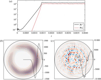
(a) Time series of
 $Re^{\ast }$
(thick black line) and
 $Re_{0}^{\ast }$
(red) for
 $Ek=10^{-8}$
,
 $Pr=10^{-2}$
and
 $Ra=1.06Ra_{c}$
. (b,c) Streamfunction (colour, snapshot) and radial profiles of the zonal velocity (snapshot, solid line, plotted according to the right-hand side axis) during (b) the growing phase at
 $t=1.36\times 10^{-3}$
and (c) the saturated phase at
 $t=1.52\times 10^{-3}$
.

Figure 4(a) shows the time series of the Reynolds number,
 $Re^{\ast }$
, and the zonal Reynolds number,
 $Re_{0}^{\ast }$
, for
 $Ek=10^{-8}$
,
 $Pr=10^{-2}$
and
 $Ra=1.06Ra_{c}$
. After a small temperature perturbation is added at
 $t=0$
, the kinetic energy grows exponentially and eventually saturates around a mean value. Despite the proximity to the onset of convection, the values of the Reynolds numbers are large in the saturated phase, on average
 $Re\approx 15200$
and
 $Re_{0}\approx 9600$
. Figure 4(b,c) show snapshots of the streamfunction during the growing phase and the saturated phase respectively. During the growth, the flow has the distinctive pattern of a thermal Rossby wave. The azimuthal modulation of the non-axisymmetric pattern is caused by the interaction of Rossby waves of different azimuthal wavenumbers. A snapshot of the zonal flow is also shown as a solid black line. The zonal flow has the familiar double jet structure seen at the onset of convection at
 $Ek=10^{-5}$
(figure 2
a). During the saturated phase, the flow is markedly different. The flow is now organised into two regions in the equatorial plane. In the inner region (
 $s<0.6$
), the pattern of the thermal Rossby waves is lost and the convective flow is vigorous with a wide range of length scales. In the outer part (
 $s>0.6$
), the velocity has a smaller amplitude and the characteristic elongated and tilted pattern of the Rossby waves is visible. This type of zonation of the convection was previously described by Sumita & Olson (Reference Sumita and Olson2000), Aubert et al. (Reference Aubert, Gillet and Cardin2003), Miyagoshi, Kageyama & Sato (Reference Miyagoshi, Kageyama and Sato2010) for Rayleigh numbers several times above critical. In the outer part, the vortex stretching term due to the slope of the boundaries is predominant over the other forces, so Rossby waves are easily excited there. The zonal flow is also modified: its radial structure is more complex with three main jets of similar radial widths, where a jet is defined by a zonal velocity of same sign. The innermost and outermost jets remain prograde while the middle jet is retrograde. The outermost prograde zonal jet is driven by the Reynolds stresses from the tilted thermal Rossby waves in the outer region.
(a)
 $Re$
as a function of
 $Ra/Ra_{c}$
for
 $Ek=10^{-8}$
and
 $Pr=10^{-2}$
. The limit between the initial value of
 $Re^{\ast }$
leading to either the decay or the growth of the solution is plotted as triangles. (b) Same as (a) for all the cases of subcritical convection (
 $Ek=10^{-8}$
,
 $Pr\in [10^{-2},10^{-1}]$
and
 $Ek=10^{-7}$
,
 $Pr=10^{-2}$
).

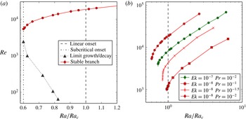
Figure 5(a) shows the values of
 $Re$
when the Rayleigh number is varied around the onset of convection for
 $Ek=10^{-8}$
and
 $Pr=10^{-2}$
. As previously noted in figure 4(a),
 $Re$
becomes large (of the order of
 $10^{4}$
) when
 $Ra$
is only just slightly increased above
 $Ra_{c}$
. Remarkably, when the Rayleigh number is decreased during a simulation from
 $Ra\geqslant Ra_{c}$
to
 $Ra<Ra_{c}$
, the convection does not decay and remains vigorous up to a value of the Rayleigh number,
 $Ra_{s}$
, where the convection abruptly shuts down. At
 $Ra=Ra_{s}$
, the value of
 $Re$
is discontinuous: for Rayleigh numbers above
 $Ra_{s}$
, we have
 $Re>5000$
, whereas for all
 $Ra$
below
 $Ra_{s}$
,
 $Re=0$
. This behaviour (
 $Ra_{s}<Ra_{c}$
) is typical of a subcritical onset of nonlinear convection. For
 $Ek=10^{-8}$
and
 $Pr=10^{-2}$
, we find that
 $Ra_{s}/Ra_{c}=0.60$
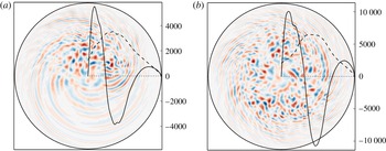
. Figure 6(a,b) show snapshots of the streamfunction for
 $Pr=10^{-2}$
and two Rayleigh numbers on the subcritical branch,
 $Ra/Ra_{c}=0.60$
and
 $0.83$
. For
 $Ra=Ra_{s}=0.60Ra_{c}$
, the convective flow is similar to the saturated case described previously in figure 4(c). The main difference is that the amplitude of the flow in the inner convective region is concentrated in a localised structure, that drifts in the azimuthal direction with time. The localisation of the convection might indicate that the system struggles to maintain convection for this Rayleigh number. However the kinetic energy of the convective and zonal flows do not decay during the entire time integration of the simulation, which corresponds to
 $200$
convective turnover time scales (where one turnover time scale is calculated as
 $1/Re_{c}$
), or equivalently,
 $2$
global thermal diffusion time scales. For larger Rayleigh numbers, the localisation in the inner convective region disappears and the convection fills all longitudes, as observed for
 $Ra=0.83Ra_{c}$
in figure 6(b). The radial profile
 $U_{s}$
is plotted in figure 6(a,b). The r.m.s. radial velocity peaks in the inner convective region, and then, monotonically decreases in the outer Rossby wave region. The boundary between the convective inner region and the outer Rossby wave region moves outwards when
 $Ra$
increases. The radial profile of the zonal flow,
 $U_{0}$
, is also plotted in figure 6(a,b). As described in the saturated case of figure 4(c), the zonal flow displays three jets in both cases. The peak of the middle retrograde jet roughly coincides with the maximum of
 $U_{s}$
. The zonal flows represent a significant portion of the total flow with the amplitude of
 $Re_{0}$
increasing from
 $0.5Re_{c}$
to
 $1.3Re_{c}$
when
 $Ra/Ra_{c}$
varies from
 $0.60$
to
 $3$
. No significant change in the flow is observed when the Rayleigh number is varied across the linear critical value
 $Ra_{c}$
, and all of the output parameters evolve continuously, similarly to
 $Re_{c}$
in figure 5(a). No continuous branch of convection is found at
 $Ra=Ra_{c}$
when the convection is started from a small perturbation as described for
 $Ek=10^{-5}$
.
Streamfunction (colour, snapshot) and radial profiles of
 $U_{s}$
(dashed line) and
 $U_{0}$
(solid line) (time averages) for
 $Ek=10^{-8}$
,
 $Pr=10^{-2}$
: (a)
 $Ra=Ra_{s}=0.60Ra_{c}$
and (b)
 $Ra=0.83Ra_{c}$
.

Within the interval
 $Ra_{s}\leqslant Ra<Ra_{c}$
, the system has two stable solutions: one is located on the subcritical branch shown in red in figure 5(a) and is found by using an initial condition with a large enough amplitude; the other solution corresponds to
 $Re=0$
and is found by starting the simulation from a small perturbation. In order to quantify how large the finite amplitude of the initial condition must be to access the subcritical branch, we perform a series of simulations where the initial condition is taken from a snapshot of the saturated solution on the subcritical branch for given parameters and we initially divide the amplitude of the velocity by a given factor. By a trial and error procedure, we determine the factor that separates a solution where the kinetic energy decays to zero from a solution where the kinetic energy grows back to the value on the subcritical branch. The limit between the values of
 $Re^{\ast }$
of the initial condition leading to either the decaying solution or the growing solution are shown in figure 5(a). As expected, we find that for values of
 $Ra$
just above
 $Ra_{s}$
, the finite amplitude of the initial condition must be much larger than for values of
 $Ra$
just below
 $Ra_{c}$
.
By varying the Prandtl number between
 $[10^{-2},10^{-1}]$
and the Ekman number between
 $[10^{-8},10^{-5}]$
, we find that subcritical convection occurs for
 $Ek=10^{-8}$
at
 $Pr\leqslant 10^{-1}$
and
 $Ek=10^{-7}$
at
 $Pr\leqslant 10^{-2}$
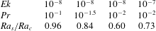
. Table 1 gives the values of
 $Ra_{s}/Ra_{c}$
for the subcritical cases and figure 5(b) shows
 $Re$
as a function of
 $Ra/Ra_{c}$
for these cases. Note that long time integrations are required to determine
 $Ra_{s}$
. The values of
 $Ra_{s}$
are obtained from simulations where the convection does not decay for the entire duration of the calculation, which is at least
 $200$
convective turnover time scales. We find that the value of
 $Re$
at
 $Ra=Ra_{s}$
is of the order of or larger than
 $10^{3}$
. The ratio
 $Ra_{s}/Ra_{c}$
decreases when
 $Ek$
decreases, and also when
 $Pr$
decreases. Consequently, our results suggest that the subcritical behaviour is amplified by low Ekman and Prandtl numbers.
Values of the ratio of the Rayleigh number at the nonlinear onset of convection to the critical Rayleigh number at the linear onset in the subcritical cases.

The subcritical behaviour of convection in internal heating models in the limit of small
 $Ek$
was anticipated from the work of Soward (Reference Soward1977), who found weakly nonlinear solutions close to the critical Rayleigh number at the linear onset predicted by the local theory of Busse (Reference Busse1970), which is significantly smaller than the true global value (Jones et al.
Reference Jones, Soward and Mussa2000). These nonlinear solutions are maintained in the subcritical domain because the zonal shear produced by nonlinear effects opposes the process of phase mixing, which is responsible for the decay of the linear solution. Subcritical convection for small Ekman numbers was also predicted by Plaut et al. (Reference Plaut, Lebranchu, Simitev and Busse2008) from a weakly nonlinear analysis of a quasi-geostrophic model with internal heating. Plaut et al. found that the bifurcation to the thermal Rossby waves changes from supercritical to subcritical for
 $Ek\leqslant 6.7\times 10^{-7}$
(in our scaling) at
 $Pr=1$
. Their analysis demonstrates that the nonlinearities in the temperature equation are responsible for the transition. These nonlinearities are produced by the interactions of the zonal flow with the temperature perturbation of the wave and by the interactions of the axisymmetric temperature with the velocity of the wave. The difference between our numerical results and the weakly nonlinear analysis of Plaut et al. (Reference Plaut, Lebranchu, Simitev and Busse2008), which predicts subcriticality for larger
 $Ek$
at
 $Pr=1$
, is possibly due to their treatment of the temperature in two dimensions. As far as we know, the numerical results of the present paper are the first to demonstrate the existence of subcritical rotating convection in a fully nonlinear model in spherical geometry. The requirements of small Ekman numbers and small Prandtl numbers (at least for
 $Ek\in [10^{-8},10^{-7}]$
) can explain why subcriticality has not been observed in previous numerical models (e.g. by Morin & Dormy (Reference Morin and Dormy2004) with QG simulations at
 $Ek=2\times 10^{-7}$
and
 $Pr=1$
). Although subcriticality in the fully 3-D system has been predicted from the work of Soward (Reference Soward1977) for small
 $Ek$
, its presence in our results might yet be a consequence of our quasi-geostrophic approximation. Future 3-D simulations will be needed to determine whether this is the case.
3.3 A hysteresis loop for
$E=10^{-6}$
and
$Pr=10^{-2}$


For
 $Ek=10^{-6}$
, the bifurcation at the onset of convection is supercritical for all the Prandtl numbers studied here (
 $Pr\in [10^{-2},10^{-1}]$
). For
 $Pr=10^{-2}$
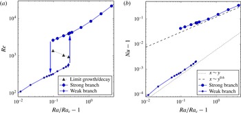
, we observe an interesting behaviour near the onset: two stable branches of convection co-exist within a limited range of Rayleigh numbers. This behaviour can be seen in the evolution of
 $Re$
and
 $Nu-1$
with
 $Ra/Ra_{c}-1$
in figure 7. On the upper branch,
 $Re$
is one order of magnitude larger than on the lower branch. We thus refer to the upper branch as strong and the lower branch as weak. The two branches are stable and co-exist for Rayleigh numbers between
 $1.09\leqslant Ra/Ra_{c}\leqslant 1.27$
. The co-existence of two stable branches for a range of
 $Ra$
leads to a hysteresis loop. The convection selects the weak or the strong branch depending on the dynamical history of the system. For instance, the system remains on the strong branch if the initial condition is taken from a simulation with
 $Ra>1.27Ra_{c}$
and
 $Ra$
is then decreased down to
 $1.09Ra_{c}$
. For
 $Ra>1.27Ra_{c}$
, only the strong branch exists according to our calculations. When the system is located on the weak branch, an increase of the Rayleigh number above
 $1.27Ra_{c}$
therefore leads the system to jump to the strong branch.
Evolution of (a)
 $Re$
and (b)
 $Nu-1$
as a function of the Rayleigh number for
 $E=10^{-6}$
and
 $Pr=10^{-2}$
.

In order to quantify the amplitude of the velocity required to jump from one branch to the other, we follow the same numerical procedure as described in § 3.2. As an initial condition, we use a snapshot of a solution on the weak branch that we multiply by a given factor and determine the initial amplitude of the flow leading to either a return to the weak branch or a growth to the strong branch. The triangles in figure 7(a) indicate the limit between the initial value of the r.m.s. velocity leading to the growth or the decay of the energy. As expected a larger amplitude of the initial velocity is required to jump to the strong branch for
 $Ra=1.09Ra_{c}$
than
 $Ra=1.27Ra_{c}$
. In fact, for
 $Ra=1.27Ra_{c}$
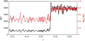
, we observe that, when the system is on the weak branch, a fluctuation of the kinetic energy can lead the system to jump to the strong branch regime. Figure 8 shows this jump in a time series of the Reynolds number,
 $Re^{\ast }$
. The two branches are well separated as there is no slow variation on the weak branch towards the strong branch, but only a sudden jump that lasts less than
 $3$
convective turnover time scales. The ratio of zonal to total Reynolds numbers (plotted according to the right axis) is approximately
 $0.45$
on the weak branch and increases to approximately
 $0.8$
after the jump to the strong branch.
Time series of
 $Re^{\ast }$
(thick black line, left axis) and
 $Re_{0}^{\ast }/Re^{\ast }$
(red, right axis) for a simulation near the edge of the hysteresis loop
 $E=10^{-6}$
,
 $Pr=10^{-2}$
and
 $Ra=1.27Ra_{c}$
.

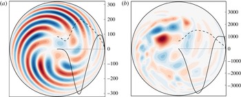
Streamfunction (colour),
 $U_{0}$
(solid line) and
 $U_{s}$
(dashed line) for
 $Ek=10^{-6}$
,
 $Pr=10^{-2}$
and
 $Ra=1.19Ra_{c}$
on (a) the weak branch and (b) the strong branch.

Typical convective flows on the weak and strong branches are shown in figure 9(a,b) for the same Rayleigh number
 $Ra=1.19Ra_{c}$
. On the weak branch, the flow consists in thermal Rossby waves. The zonal flow has a double jet structure and its amplitude is comparable to the amplitude of the radial flow. The characteristics of this flow are similar to the case described near the onset of convection for
 $Ek=10^{-5}$
(§ 3.1). On the strong branch, the thermal Rossby waves are not visible anymore and a wide range of length scales are observed. The zonal flow has a larger amplitude than the radial velocity. Not only do the solutions look different on the two branches, the global properties of the convection also follow different scaling laws with the input parameters. The evolution of
 $Nu$
with the Rayleigh number (figure 7
b) is less steep on the strong branch compared with the weak branch. On the weak branch we find that the points approximately follow a power law
 $Nu\sim (Ra/Ra_{c}-1)^{\unicode[STIX]{x1D6FC}}$
with
 $\unicode[STIX]{x1D6FC}=1$
, whereas on the strong branch
 $\unicode[STIX]{x1D6FC}=0.6$
.
3.4 Nonlinear oscillations for
$E=10^{-7}$
and
$Pr=10^{-1}$


For
 $E=10^{-7}$
and
 $Pr=10^{-1}$
, we observe an interesting behaviour between the linear onset of convection and the saturated branch of convection, for values of
 $Ra$
between
 $Ra_{c}$
and
 $1.025Ra_{c}$
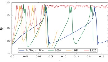
. This behaviour is best observed in the time series of
 $Re^{\ast }$
shown in figure 10 for Rayleigh numbers in this interval.
 $Re^{\ast }$
first grows at a rate that depends on
 $Ra$
and then reaches a value of approximately
 $400$
. After a few fluctuations around this mean value,
 $Re^{\ast }$
decreases rapidly. The system subsequently enters a new growing phase and the oscillation repeats itself. The duration of the oscillation depends on the growth rate, and so, larger Rayleigh numbers have shorter period. For
 $Ra=1.025Ra_{c}$
, the system eventually stays on the saturated branch after a few oscillations, after which it never goes back to the oscillating phase.
Time series of the Reynolds number,
 $Re^{\ast }$
, for
 $E=10^{-7}$
and
 $Pr=10^{-1}$
and Rayleigh numbers near the onset.

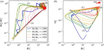
Phase diagram of (a)
 $Re_{0}^{\ast }/Re_{c}^{\ast }$
versus
 $Re_{c}^{\ast }$
and (b)
 $\unicode[STIX]{x1D6E9}_{0}^{\ast }$
versus
 $Re_{c}^{\ast }$
for the same time series as figure 10.

This behaviour is similar to nonlinear oscillations such as relaxation oscillations found in many dynamical systems (Fauve Reference Fauve, Godrèche and Manneville1998). These oscillations are quasi-periodic and may be better understood using phase diagrams. Figure 11(a) shows the phase diagram of the ratio of the zonal to convective Reynolds numbers,
 $Re_{0}^{\ast }/Re_{c}^{\ast }$
, versus the convective Reynolds number,
 $Re_{c}^{\ast }$
, for the same time series as figure 10. Figure 11(b) shows the phase diagram for the r.m.s. axisymmetric temperature,
 $\unicode[STIX]{x1D6E9}_{0}^{\ast }$
, versus
 $Re_{c}^{\ast }$
. During the exponential growing phase
 $Re_{c}^{\ast }$
(labelled (A)), all trajectories follow the same path and
 $Re_{0}^{\ast }$
increases as the square of
 $Re_{c}^{\ast }$
, in agreement with weakly nonlinear analysis near the onset of convection (see § 3.1). The system reaches a maximum (B), where
 $Re_{0}^{\ast }$
has a similar amplitude to
 $Re_{c}^{\ast }$
. A dissipative phase (C) then follows during which
 $Re_{0}^{\ast }$
and
 $Re_{c}^{\ast }$
initially decay at the same rate. The three quantities,
 $Re_{c}^{\ast }$
,
 $Re_{0}^{\ast }$
and
 $\unicode[STIX]{x1D6E9}_{0}^{\ast }$
, all start to decay at the same time. While
 $Re_{c}^{\ast }$
and
 $Re_{0}^{\ast }$
enter together the growing phase (A), the decay of
 $\unicode[STIX]{x1D6E9}_{0}^{\ast }$
persists for longer. The three phases (A, B, C) are fairly similar for all the Rayleigh numbers, although the system can follow different trajectories during the dissipative phase. For the largest Rayleigh number (
 $Ra=1.025Ra_{c}$
), the system exits the oscillating regime to reach a stagnation point (D), which is clearly distinct from the phase (B) according to the measurements of
 $\unicode[STIX]{x1D6E9}_{0}^{\ast }$
. During the phase (D), the characteristics of the flow are similar than the ones described in § 3.2 for
 $Ek=10^{-8}$
, so this saturated regime corresponds to the strong branch of convection.
Relaxation oscillations are a well-known phenomenon in rotating spherical convection for Rayleigh numbers a few times above onset (e.g. Grote & Busse Reference Grote and Busse2001; Morin & Dormy Reference Morin and Dormy2004; Teed et al.
Reference Teed, Jones and Hollerbach2012). However, unlike in these higher
 $Ra$
relaxation oscillations, which are caused by the disruption of the convection by the zonal flow and the axisymmetric temperature gradient (Teed et al.
Reference Teed, Jones and Hollerbach2012), we do not observe here a time lag between the maximum of
 $Re_{0}^{\ast }$
and
 $Re_{c}^{\ast }$
, so the oscillations of figure 10 are produced by a different mechanism.
Snapshots of the streamfunction and the zonal flow for
 $E=10^{-7}$
,
 $Pr=0.1$
and
 $Ra=1.004Ra_{c}$
. Between the first and last snapshots, a time corresponding to about
 $10^{4}$
rotation periods has elapsed.

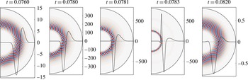
Figure 12 shows a series of snapshots of the streamfunction (colour) and the zonal flow (solid black line) during the different phases of the nonlinear oscillation for
 $Ra=1.004Ra_{c}$
. During the growing phase (A) (
 $t=0.076$
), the flow consists of a thermal Rossby wave and a double zonal jet, both developing around the radius
 $s=0.5$
, reminiscent of the solution on the weak branch. When the system reaches the maximum (B) (
 $t=0.078$
), the thermal Rossby wave and the zonal flow drift inwards. A narrow prograde zonal jet starts to develop around
 $s=0.35$
(
 $t=0.0781$
) and rapidly gains a very large amplitude (
 $t=0.0783$
). The non-axisymmetric flow is maximum inside the narrow newly formed prograde jet and keeps the same azimuthal wavenumber as the thermal Rossby wave. The amplitudes of both the zonal and non-axisymmetric flows then decay rapidly (phase (C)). A new oscillation begins with the growth of a thermal Rossby wave and its associated double zonal jet around the radius
 $s=0.5$
, while the zonal flow of the past oscillation finishes to be dissipated (
 $t=0.082$
). The inward migration of the non-axisymmetric and zonal flows during the phase (B) is probably the cause for the disruption of the convection and the oscillatory behaviour. The mechanism responsible for the inward migration remains unclear as the competitive effects that either inhibit (
 $\unicode[STIX]{x1D6FD}$
effect) or promote (gravity along
 $s$
) convection depend on radius.
Space–time diagram of (a)
 $\overline{u_{\unicode[STIX]{x1D719}}}$
and (b)
 $\unicode[STIX]{x1D6E5}$
for
 $E=10^{-7}$
,
 $Pr=0.1$
and
 $Ra=1.004Ra_{c}$
.

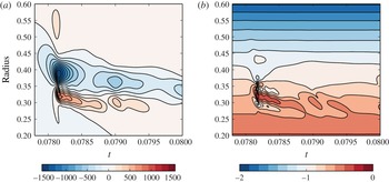
We note that a secondary effect might arise from the inward migration of the zonal flow in the form of a shear instability. Indeed, the Rossby wave that is confined within the intense narrow prograde jet (
 $t=0.0783$
in figure 12) could have been excited by such an instability. A sufficient and necessary condition for the barotropic instability of a shear flow in a inviscid Boussinesq fluid is that the quantity
 $\unicode[STIX]{x1D6E5}=2\unicode[STIX]{x1D6FD}Ek^{-1}-\text{d}\overline{\unicode[STIX]{x1D701}}/\text{d}s$
, where
 $\overline{\unicode[STIX]{x1D701}}=\text{d}\overline{u_{\unicode[STIX]{x1D719}}}/\text{d}s+\overline{u_{\unicode[STIX]{x1D719}}}/s$
, changes sign at some radius (Kuo Reference Kuo1949; Ingersoll & Pollard Reference Ingersoll and Pollard1982). Guervilly, Cardin & Schaeffer (Reference Guervilly, Cardin and Schaeffer2012) showed that the threshold of the instability obtained with numerical simulations at finite
 $Ek$
approaches asymptotically the inviscid theoretical prediction as the Ekman number is decreased and a good quantitative agreement is obtained at
 $Ek=10^{-7}$
. Figure 13 shows the space–time diagram of
 $\overline{u_{\unicode[STIX]{x1D719}}}$
and
 $\unicode[STIX]{x1D6E5}$
between the time
 $t=0.0778$
and
 $t=0.08$
for the same simulation as figure 12.
 $\unicode[STIX]{x1D6E5}$
is always negative, although it comes close to zero when the narrow prograde jet is at its maximum. It is nonetheless possible that the linear stability criteria is violated, but this cannot be strictly identified in the nonlinear simulation because the zonal flow would be rapidly modified by the growth of the shear instability. We emphasise that if the zonal flow is shear unstable, it is a secondary effect and not the cause of the inward migration.
We find similar nonlinear oscillations in the vicinity of the linear onset of convection for
 $Ek=10^{-6}$
and
 $Pr=10^{-1}$
, but in a narrower window of Rayleigh numbers (between
 $Ra=Ra_{c}$
and
 $Ra=1.0015Ra_{c}$
). For larger Rayleigh numbers, the convection is similar to the solution found on the weak branch with thermal Rossby waves. This therefore indicates that the nonlinear oscillations are not a consequence of the existence of a strong branch of convection.
4 Discussion
We have studied rotating thermal convection driven by internal heating in a full sphere near the onset of convection for values of the Prandtl number relevant for liquid metals (
 $Pr\in [10^{-2},10^{-1}]$
) and low Ekman numbers (
 $Ek\in [10^{-8},10^{-5}]$
). We have used a hybrid numerical model that couples a quasi-geostrophic approximation for the velocity to a fully 3-D temperature field. The model includes Ekman pumping to mimic no-slip boundary conditions. Our main finding is the identification of two distinct branches of rapidly rotating convection: (i) a weak branch for
 $Ek\geqslant \mathit{O}(10^{-6})$
that is linked to the linear onset of convection (at
 $Ra=Ra_{c}$
) by a supercritical bifurcation and (ii) a strong branch for lower Ekman numbers that is discontinuous at the onset and can only be reached by using finite-amplitude perturbations as initial conditions. On the weak branch for
 $Ra$
just above
 $Ra_{c}$
, the flow consists of the interaction of thermal Rossby waves and a zonal flow with a double jet structure, and has been extensively documented in the literature (e.g. Busse & Hood Reference Busse and Hood1982; Zhang Reference Zhang1992a
). The amplitude of the zonal flow on this branch near onset is smaller than the amplitude of the convective (i.e. non-axisymmetric) velocity. On the strong branch, the flow contains a wide range of length scales and its Reynolds number
 $Re$
exceeds
 $10^{3}$
. The zonal flow has multiple jets for
 $Ek\leqslant 10^{-7}$
and its amplitude is comparable to or larger than the convective velocity, even near the nonlinear onset of convection. For
 $Ek=10^{-5}$
, the transition from quasi-steady convection to time-dependent convection that produces an abrupt kink in the evolution of
 $Re$
and
 $Nu$
as a function of
 $Ra$
(see figure 3(a,b) corresponds perhaps to the continuous transition from the weak to the strong branch. This transition has been observed in previous 3-D models (Tilgner & Busse Reference Tilgner and Busse1997; Simitev & Busse Reference Simitev and Busse2003), so the existence of the two branches of convection might not be specific to the quasi-geostrophic model. When the viscous effects become smaller, the transition between the two branches becomes discontinuous leading to the existence of two distinct branches, which allows us to observe a hysteresis loop for
 $Ek=10^{-6}$
and
 $Pr=10^{-2}$
, where the onset of the strong branch occurs at
 $Ra_{s}=1.09Ra_{c}$
.
For yet lower Ekman numbers, we find that the strong branch becomes subcritical with
 $Ra_{s}<Ra_{c}$
. In this case, we did not find the weak branch that is continuous at the linear onset. The parameters
 $(Ek,Pr)$
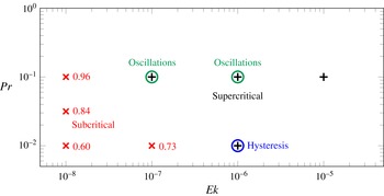
for which we observe subcritical convection are denoted by red crosses in the regime diagram shown in figure 14. The ratio
 $Ra_{s}/Ra_{c}$
is indicated next to each point and decreases with the Ekman number and the Prandtl number. To the best of our knowledge, this is the first time that subcriticality is reported in thermal convection in a rotating sphere. It is possible that this behaviour is specific to the quasi-geostrophic model, as the nonlinear bifurcation might be sensitive to the treatment of the axial velocity for instance. Nevertheless subcritical convection in the fully 3-D system has been expected from the work of Soward (Reference Soward1977) in the asymptotic limit
 $Ek\rightarrow 0$
(see figure 3.2 of Proctor (Reference Proctor1994)). Soward found that weakly nonlinear solutions exist close to the critical Rayleigh number predicted by the local asymptotic theory,
 $Ra_{c}^{l}$
(Busse Reference Busse1970), which is smaller than the critical Rayleigh number of the global asymptotic theory,
 $Ra_{c}^{g}$
(Jones et al.
Reference Jones, Soward and Mussa2000). The discrepancy between local and global asymptotic theories increases at small Prandtl numbers (see appendix A), so it is perhaps unsurprising that the subcriticality is amplified in this case in our simulations. For
 $Pr=10^{-2}$
,
 $Ra_{c}^{l}/Ra_{c}^{g}=0.03$
, while
 $Ra_{c}^{l}/Ra_{c}^{g}=0.82$
for
 $Pr=1$
(Jones et al.
Reference Jones, Soward and Mussa2000). For
 $Ek=10^{-8}$
and
 $Pr=10^{-2}$
, we find that
 $Ra_{s}/Ra_{c}=0.60$
, which could indicate that our simulations are still a long way from the asymptotic limit.
Regime diagram showing the location of the subcritical convection (red cross) and supercritical bifurcation at the onset of nonlinear convection (black plus) identified with our hybrid model. The value annotated next to the subcritical cases gives the ratio
 $Ra_{s}/Ra_{c}$
.

The region of intermediate Ekman numbers, between supercritical bifurcation at
 $Ek\geqslant 10^{-5}$
and subcritical convection at
 $Ek\lesssim 10^{-7}$
, displays interesting behaviours such as hysteresis. We also observe nonlinear oscillations for Rayleigh numbers just above the linear onset and up to
 $Ra/Ra_{c}=1.025$
for
 $Ek=10^{-7}-10^{-6}$
and
 $Pr=10^{-1}$
. For
 $Ek=10^{-7}$
, the dynamical regime is located on the strong branch for larger Rayleigh numbers, so in this case
 $Ra_{s}\approx Ra_{c}$
. For
 $Ek=10^{-6}$
however, the solution at larger
 $Ra$
is similar to the convection at larger Ekman numbers. In both cases, the nonlinear oscillations are due to an inward migration of the convective region, whose cause remains unexplained (see figure 12).
The results presented in this paper rely on a quasi-geostrophic model of the velocity and a 3-D model of the temperature, which allowed us to compute small Ekman numbers currently out of reach of 3-D models (e.g. Miyagoshi et al.
Reference Miyagoshi, Kageyama and Sato2010; Matsui et al.
Reference Matsui, Heien, Aubert, Aurnou, Avery, Brown, Buffett, Busse, Christensen and Davies2016; Yadav et al.
Reference Yadav, Gastine, Christensen, Duarte and Reiners2016). Assuming that our results are not specific to the hybrid model, it would be difficult to observe subcriticality for 3-D models in the near future, but it might be possible to observe the discontinuous transition between the two branches at low enough Prandtl numbers for
 $Ek=10^{-6}$
for instance.
In order to extrapolate the results of numerical models to natural bodies such as the Earth’s core, the models must capture the proper convection branch. Indeed here, we find that the scaling of the Nusselt number with the parameters are significantly different on the weak and strong branches (see figure 7
b for the hysteresis). In this paper, we do not derive scaling laws for the strong branch for all the studied parameters because it is unclear whether the points actually follow a power law for the small values of
 $Ra/Ra_{c}$
studied here. The zonal flows and the scaling of the Reynolds and Nusselt numbers at higher Rayleigh numbers will be addressed in a forthcoming study.
Many questions remain unanswered in our study and, in particular, we have not identified the physical mechanisms leading to subcritical convection in our simulations and controlling the value of
 $Ra_{s}$
. The zonal flow and/or the axisymmetric temperature are probably essential for the subcriticality (Plaut et al.
Reference Plaut, Lebranchu, Simitev and Busse2008). Whether the temperature needs to be treated in 3-D to observe this behaviour is unclear. The role played by the type of thermal heating also remains an open question. Following the argument that the distinction between the local and global asymptotic theories yields the existence of subcritical convection, Gillet & Jones (Reference Gillet and Jones2006) argue that the case of differential heating might well always be supercritical because no such distinction exists in this case.
The context of the present work is the study of the fluid dynamics in planetary liquid cores. It is of interest to note that, in this context, the possibility of the subcritical behaviour of rapidly rotating convection due to the action of a magnetic field is an active area of research (e.g. Sreenivasan & Jones Reference Sreenivasan and Jones2011; Dormy Reference Dormy2016). In magnetoconvection, where a magnetic field is imposed, the Lorentz force can counteract the inhibiting action of the Coriolis force on the convection and leads to a reduced onset of convection (Chandrasekhar Reference Chandrasekhar1961; Eltayeb Reference Eltayeb1972; Fearn Reference Fearn1979). In dynamo simulations, the magnetic field is sustained by the convective flow and saturates due to the feedback of Lorentz forces on the flow. When a strong magnetic field is sustained, the Lorentz forces can strongly affect the flow and it is then possible that the Rayleigh number required to maintain the dynamo falls below the Rayleigh number required to excite the dynamo in the first place at the dynamo onset (which occurs at
 $Ra>Ra_{c}$
). Examples of this subcritical behaviour below the dynamo onset have been reported by Kuang, Jiang & Wang (Reference Kuang, Jiang and Wang2008), Morin & Dormy (Reference Morin and Dormy2009), Sreenivasan & Jones (Reference Sreenivasan and Jones2011), Hori & Wicht (Reference Hori and Wicht2013), and have been used as a possible explanation for the sudden termination of the Martian dynamo. However in these examples of convectively driven dynamos in a spherical geometry, the Rayleigh number always exceeds
 $Ra_{c}$
. As far as we know, the only example of a dynamo simulation operating below
 $Ra_{c}$
was found by Stellmach & Hansen (Reference Stellmach and Hansen2004) in a planar model of rotating convection. It would be of great interest to study the dynamo action produced by the flows on the strong hydrodynamical branch identified in this paper, and whether the Lorentz force can push the system to remain convective at yet smaller Rayleigh numbers as suggested for instance by Roberts (Reference Roberts1988).
Acknowledgements
C.G. was supported by the Natural Environment Research Council under grant NE/M017893/1. P.C. acknowledges the Agence Nationale de la Recherche for supporting this project under grant ANR TuDy. This work was undertaken on ARC1 and ARC2 of the HPC facilities at the University of Leeds, on TOPSY of the HPC facilities at Newcastle University and on the Froggy platform of the CIMENT infrastructure (https://ciment.ujf-grenoble.fr). The CIMENT infrastructure is supported by the Rhône-Alpes region (GRANT CPER07_13 CIRA), the OSUG@2020 labex (reference ANR10 LABX56) and the Equip@Meso project (reference ANR-10-EQPX-29-01). ISTerre is part of Labex OSUG@2020 (ANR10 LABX56). We are grateful to E. Dormy, A. Soward, T. Wood and the Geodynamo group in Grenoble for helpful discussions and to the anonymous referees for suggestions that have improved the manuscript.
Appendix A. Linear onset of convection
The onset of thermal convection in a rotating sphere with internal heating in the asymptotic limit
 $Ek\ll 1$
and
 $Ek/Pr\ll 1$
was studied analytically by Roberts (Reference Roberts1968), Busse (Reference Busse1970), Yano (Reference Yano1992), Jones et al. (Reference Jones, Soward and Mussa2000). In this limit, the most unstable mode of convection develops in the form of columnar structures aligned with the rotation axis, which are called thermal Rossby waves. They develop around a radius
 $s\approx 0.5$
. Using a local perturbative study, Busse (Reference Busse1970) determined the analytical dependence of the critical parameters at the onset of convection as a function of
 $Ek$
and
 $Pr$
,
 $$\begin{eqnarray}\displaystyle & \displaystyle Ra_{c}^{l}=C_{r}\left(\frac{Pr}{1+Pr}\right)^{4/3}Ek^{-4/3}, & \displaystyle\end{eqnarray}$$
 $$\begin{eqnarray}\displaystyle & \displaystyle m_{c}^{l}=C_{m}\left(\frac{Pr}{1+Pr}\right)^{1/3}Ek^{-1/3}, & \displaystyle\end{eqnarray}$$
 $$\begin{eqnarray}\displaystyle & \displaystyle \unicode[STIX]{x1D714}_{c}^{l}=C_{\unicode[STIX]{x1D714}}\left(Pr(1+Pr)^{2}\right)^{-1/3}Ek^{-2/3}, & \displaystyle\end{eqnarray}$$
 $Ra_{c}^{l}$
is the critical Rayleigh number,
 $m_{c}^{l}$
the marginally stable azimuthal wavenumber,
 $\unicode[STIX]{x1D714}_{c}^{l}$
its frequency and
 $C_{r}$
,
 $C_{m}$
and
 $C_{\unicode[STIX]{x1D714}}$
are constants. However, Soward (Reference Soward1977) showed that small disturbances decay with time for values of the Rayleigh number just above the local critical Rayleigh number (A 1). Jones et al. (Reference Jones, Soward and Mussa2000) calculated the true value of the critical Rayleigh number from the global asymptotic theory,
 $Ra_{c}^{g}$
, and found that it is significantly larger than
 $Ra_{c}^{l}$
.
In order to benchmark our hybrid model, we have performed calculations with a linearised version of the code and compared the results with the values of the global asymptotic theory of Jones et al. (Reference Jones, Soward and Mussa2000) for
 $Pr\in [10^{-2},1]$
. We study the onset of the thermal Rossby waves, so we restrict our study to the domain of small Ekman numbers where they are preferred over the equatorially attached modes, i.e.
 $Ek\leqslant 10^{-4}$
for
 $Pr=10^{-1}$
and
 $Ek\leqslant 10^{-6}$
for
 $Pr=10^{-2}$
(see § 1). We also compare the dependence of the critical parameters on
 $Pr$
with the power laws of the local theory (A 1)–(A 3). We calculated the linear onset for
 $Pr=1$
at
 $Ek\in [10^{-6},10^{-5}]$
to compare our results with published numerical results obtained with a fully 3-D model (Dormy et al.
Reference Dormy, Soward, Jones, Jault and Cardin2004) and a quasi-geostrophic description, where the temperature is also treated in two dimensions (hereafter denoted QG–2-D) (Aubert Reference Aubert2001). In these previous studies, the critical parameters for convection driven by internal heating were only published for
 $Pr=1$
and the model includes an inner core of radius
 $0.35$
. The boundary conditions for the 3-D model of Dormy et al. (Reference Dormy, Soward, Jones, Jault and Cardin2004) are no slip, while the QG–2-D model of Aubert (Reference Aubert2001) neglects the Ekman pumping.
Critical parameters at the linear onset of convection calculated with a linearised version of the hybrid QG–3-D numerical code.

Critical parameters for the linear onset of convection as a function of
 $Ek$
for
 $Pr=1$
computed with our model (hybrid QG–3-D), with the 3-D model of Dormy et al. (Reference Dormy, Soward, Jones, Jault and Cardin2004) and the quasi-geostrophic model of Aubert (Reference Aubert2001). These numerical results are compared with the asymptotic results of Jones et al. (Reference Jones, Soward and Mussa2000). The dashed grey line represents the asymptotic results including first-order correction (Jones et al.
Reference Jones, Soward and Mussa2000).

The critical parameters calculated with our code
 $(Ra_{c},m_{c},\unicode[STIX]{x1D714}_{c})$
are given in table 2. As the Ekman number is decreased,
 $Ra_{c}$
gets closer to the asymptotic value
 $Ra_{c}^{g}$
for all
 $Pr$
. The values of the critical parameters are plotted as a function of
 $Ek$
in figure 15 for
 $Pr=1$
. The three critical parameters computed with our hybrid model tend towards the asymptotic values of the global stability analysis when
 $Ek$
decreases. The critical Rayleigh number of our model is higher than the values obtained with both the 3-D and QG–2-D models. This is expected because of the stabilising effect of the axial rigidity imposed by the quasi-geostrophic formulation, while the 3-D solution keeps a large-scale
 $z$
dependence (Gillet & Jones Reference Gillet and Jones2006). Furthermore, our hybrid approach includes the axial diffusion of the temperature, which is neglected in the QG–2-D model. The
 $z$
-average of the buoyancy force is thus weaker in our hybrid approach, so
 $Ra_{c}$
is necessarily larger. The marginally stable mode
 $m_{c}$
is smaller in our hybrid model compared with the asymptotic results. Again, this is consistent with the axial rigidity of the quasi-geostrophic flow, which requires the convection to first develop at a slightly smaller critical radius, thereby selecting a smaller
 $m_{c}$
.
Critical parameters for the linear onset of convection as a function of
 $Pr$
computed with our hybrid QG model and compared with the asymptotic results of Jones et al. (Reference Jones, Soward and Mussa2000) (global theory) and Busse (Reference Busse1970) (local theory).

The critical parameters
 $(Ra_{c},m_{c},\unicode[STIX]{x1D714}_{c})$
are plotted as a function of
 $Pr$
in figure 16. Our hybrid model follows well the trend of the global asymptotic theory for the three critical parameters. Convection at smaller
 $Pr$
develops on larger scales at the onset. Accordingly, the critical frequency is larger (e.g. Jones Reference Jones and Schubert2007). These results agree reasonably well with the trends given by the power laws of the local theory for
 $m_{c}^{l}$
and
 $\unicode[STIX]{x1D714}_{c}^{l}$
(A 2)–(A 3) when
 $Pr<0.1$
, but the prefactors differ significantly. The critical Rayleigh number given by both our numerical results and the global asymptotic results differs greatly from the prediction of the local theory (
 $Ra_{c}^{l}\propto Pr^{4/3}$
when
 $Pr\ll 1$
), as already observed by Zhang (Reference Zhang1992a
). The discrepancy with
 $Ra_{c}^{l}$
(A 1) increases as the Prandtl number decreases: the difference between local and global critical Rayleigh number is nearly two orders of magnitude for
 $Pr=10^{-2}$
. Zhang (Reference Zhang1992a
) attributed this discrepancy to the tilt of the thermal Rossby waves, which is more pronounced for small
 $Pr$
.