1 Introduction
1.1 Statement of results
Let
 $k\geqslant 4$
be an even integer and let
 $E_{k}(z)$
denote the usual holomorphic weight
 $k$
Eisenstein series defined by
 $$\begin{eqnarray}E_{k}(z)=\mathop{\sum }_{\unicode[STIX]{x1D6FE}\in \unicode[STIX]{x1D6E4}_{\infty }\backslash \unicode[STIX]{x1D6E4}}j(\unicode[STIX]{x1D6FE},z)^{-k}=\frac{1}{2}\mathop{\sum }_{(c,d)=1}\frac{1}{(cz+d)^{k}},\end{eqnarray}$$
where
 $\unicode[STIX]{x1D6E4}=\text{PSL}_{2}(\mathbb{Z})$
,
 $\unicode[STIX]{x1D6E4}_{\infty }\subset \unicode[STIX]{x1D6E4}$
is the stabilizer of
 $\infty$
, and
 $j(\unicode[STIX]{x1D6FE},z)=cz+d$
for
 $\unicode[STIX]{x1D6FE}=(\!\begin{smallmatrix}a & b\\ c & d\end{smallmatrix}\!)$
.
Let
 ${\mathcal{F}}$
denote the closure of the standard fundamental domain for
 $\unicode[STIX]{x1D6E4}\backslash \mathbb{H}$
, namely
 ${\mathcal{F}}=\{z\in \mathbb{H}:|z|\geqslant 1,\text{and }|x|\leqslant 1/2\}$
. Rankin and Swinnerton-Dyer [Reference Rankin and Swinnerton-Dyer13] showed all the zeros of
 $E_{k}$
in
 ${\mathcal{F}}$
lie on the bottom arc
 $|z|=1$
.
In this paper, we study the zeros of the weight
 $k+\ell$
cusp forms defined by
 $$\begin{eqnarray}\unicode[STIX]{x1D6E5}_{k,\ell }=E_{k}E_{\ell }-E_{k+\ell }.\end{eqnarray}$$
In a few special cases,
 $\unicode[STIX]{x1D6E5}_{k,\ell }$
vanishes identically, namely when (and only when)
 $k+\ell \in \{8,10,14\}$
. For the remainder of this paper, we take the convention that
 $k+\ell \geqslant 16$
to avoid these trivial cusp forms. By symmetry, we shall assume
 $k\geqslant \ell$
.
The functions
 $\unicode[STIX]{x1D6E5}_{k,\ell }$
are interesting to study for a number of reasons. The most basic motivation comes from the fact that
 $\unicode[STIX]{x1D6E5}_{k,\ell }$
are (arguably) the easiest cusp forms to construct explicitly. In contrast, the Hecke eigenforms are rather more difficult to construct for large weights. A more advanced motivation comes from the quantum unique ergodicity (QUE) conjecture of Rudnick and Sarnak [Reference Rudnick and Sarnak15], which is an equidistribution statement for Hecke–Maass cusp forms of large Laplace eigenvalue and for holomorphic Hecke cusp forms of large weight. Holowinsky and Soundararajan [Reference Holowinsky and Soundararajan6] have proven QUE for holomorphic forms. Meanwhile, QUE for Maass forms was proved by Lindenstrauss [Reference Lindenstrauss10] and Soundararajan [Reference Soundararajan16]. In fact, in an even earlier paper, Luo and Sarnak [Reference Luo and Sarnak11] proved QUE for Eisenstein series in the spectral aspect. One may wonder if there is an analog of QUE for large weight Eisenstein series. Of course,
 $E_{k}^{2}$
is not a cusp form, so it is natural to project this form onto the cuspidal subspace, which is precisely
 $\unicode[STIX]{x1D6E5}_{k,k}$
. It is an obvious generalization to examine
 $\unicode[STIX]{x1D6E5}_{k,\ell }$
for general
 $k,\ell$
.
Many authors have studied the zeros of modular forms, including [Reference Asai, Kaneko and Ninomiya1–Reference Ghosh and Sarnak3, Reference Gun5, Reference Kohnen9, Reference Nozaki12, Reference Rankin and Swinnerton-Dyer13].
In general, we are interested in how these cusp forms
 $\unicode[STIX]{x1D6E5}_{k,\ell }$
behave. On the one hand, one may expect that
 $\unicode[STIX]{x1D6E5}_{k,\ell }$
has properties similar to a random linear combination of Hecke cusp forms of weight
 $k+\ell$
. If so, then one would expect that its zeros would equidistribute in the fundamental domain as the zeros of Hecke cusp forms do, as shown in the work of Rudnick [Reference Rudnick14] and Holowinsky and Soundararajan [Reference Holowinsky and Soundararajan6]. In contrast to this naive guess, we have the following.
Conjecture 1.1. All the zeros of
 $\unicode[STIX]{x1D6E5}_{k,\ell }$
lying in the standard fundamental domain are on the boundary,
 $|z|=1$
or
 $x=\pm 1/2$
.
This conjecture was born out of numerical evidence for
 $k,\ell \leqslant 100$
. Our main result in this paper proves the conjecture for
 $\ell$
sufficiently large.
Theorem 1.2. There exists an effective constant
 $L$
so that if
 $k\geqslant \ell \geqslant L$
, then all the zeros of
 $\unicode[STIX]{x1D6E5}_{k,\ell }$
in
 ${\mathcal{F}}$
lie on its boundary.
The zeros naturally split up into those on the arc, with
 $|z|=1$
, and those on the sides, with
 $x=\pm 1/2$
(there may also be “trivial” zeros at
 $\unicode[STIX]{x1D70C}=\text{e}^{\unicode[STIX]{x1D70B}\text{i}/3}$
and
 $\text{i}$
which are guaranteed by the valence formula depending on the value of
 $k+\ell$
modulo
 $12$
, which we do not count in this discussion).
One of the curious features of the functions
 $\unicode[STIX]{x1D6E5}_{k,\ell }$
is that the relative proportion of zeros on the arc and on the sides depends strongly on the relative sizes of
 $k$
and
 $\ell$
. In particular, in one extreme direction if
 $k=\ell$
then it appears all the zeros are on the sides. In the opposite extreme, if
 $\ell =4$
and
 $k\geqslant 12$
, then all the zeros are apparently on the arc.
Given
 $k$
and
 $\ell$
, define
 $A_{k,\ell }$
to be the number of zeros of
 $\unicode[STIX]{x1D6E5}_{k,\ell }$
on the arc
 $\{\text{e}^{\text{i}\unicode[STIX]{x1D703}}:\unicode[STIX]{x1D70B}/3<\unicode[STIX]{x1D703}<\unicode[STIX]{x1D70B}/2\}$
, and
 $B_{k,\ell }$
to be the number of zeros on the side
 $x=1/2$
,
 $y>\sqrt{3}/2$
. The number of zeros of a weight
 $k+\ell$
modular form is dictated by the valence formula:
 $$\begin{eqnarray}\frac{k+\ell }{12}=\frac{1}{2}v_{i}(f)+\frac{1}{3}v_{\unicode[STIX]{x1D70C}}(f)+v_{\infty }(f)+\underset{z\neq i,\unicode[STIX]{x1D70C}}{\sum }v_{z}(f),\end{eqnarray}$$
where the sum is taken over all
 $z\in \unicode[STIX]{x1D6E4}\backslash \mathbb{H}$
, with
 $z$
not equivalent to
 $\text{i},\unicode[STIX]{x1D70C}$
, and
 $v_{i}(f)$
,
 $v_{\unicode[STIX]{x1D70C}}(f)$
, and
 $v_{\infty }(f)$
are the orders of vanishing of
 $f$
at
 $\text{i}$
,
 $\unicode[STIX]{x1D70C}$
, and
 $\infty$
, respectively.
Since
 $\unicode[STIX]{x1D6E5}_{k,\ell }$
is a cusp form, we know that
 $v_{\infty }(\unicode[STIX]{x1D6E5}_{k,\ell })\geqslant 1$
, and in proving Conjecture 1.1, we show that this inequality is an equality. This leads us to reformulate Conjecture 1.1 as the following formula:
 $$\begin{eqnarray}A_{k,\ell }+B_{k,\ell }=\frac{k+\ell }{12}-\frac{1}{2}v_{i}(\unicode[STIX]{x1D6E5}_{k,\ell })-\frac{1}{3}v_{\unicode[STIX]{x1D70C}}(\unicode[STIX]{x1D6E5}_{k,\ell })-1.\end{eqnarray}$$
Let us agree to call the zeros at
 $i$
,
 $\unicode[STIX]{x1D70C}$
, and
 $\infty$
, guaranteed to exist by the valence formula, the trivial zeros, and the rest of the zeros the non-trivial zeros.
Conjecture 1.3. For
 $k\geqslant 14$
, all of the zeros of
 $\unicode[STIX]{x1D6E5}_{k,4}$
,
 $\unicode[STIX]{x1D6E5}_{k,6}$
, and
 $\unicode[STIX]{x1D6E5}_{k,8}$
in the fundamental domain lie on the arc
 $|z|=1$
.
Proposition 1.4. For
 $\ell$
large enough, each of
 $\unicode[STIX]{x1D6E5}_{\ell ,\ell }$
,
 $\unicode[STIX]{x1D6E5}_{\ell +2,\ell }$
,
 $\unicode[STIX]{x1D6E5}_{\ell +4,\ell }$
,
 $\unicode[STIX]{x1D6E5}_{\ell +6,\ell }$
, and
 $\unicode[STIX]{x1D6E5}_{\ell +10,\ell }$
has its non-trivial zeros on the sides
 $x=\pm 1/2$
. For
 $\ell$
large,
 $\unicode[STIX]{x1D6E5}_{\ell +8,\ell }$
has one non-trivial zero on the arc
 $|z|=1$
, and all the rest on the sides
 $x=\pm 1/2$
.
These special cases exemplify a more general pattern that when
 $k-\ell$
is large,
 $\unicode[STIX]{x1D6E5}_{k,\ell }$
tends to have more zeros on the arc, while when
 $k-\ell$
is small,
 $\unicode[STIX]{x1D6E5}_{k,\ell }$
tends to have more zeros on the sides.
In this paper, we shall produce tight bounds on the sizes of
 $A_{k,\ell }$
and
 $B_{k,\ell }$
, culminating in exact formulas for these quantities. Since the formulas are somewhat complicated and break into cases, we shall proceed in stages, giving more accurate estimates as we go.
As a starting point, we state the following.
Proposition 1.5. For
 $k\geqslant \ell \geqslant 14$
, we have
 $A_{k,\ell }=(k-\ell )/12+O(1)$
, and
 $B_{k,\ell }=2\ell /12+O(1)$
, where the implied constants are absolute (that is, uniform in
 $k,\ell$
).
Since the total number of zeros of a weight
 $k\,+\,\ell$
modular form is
 $(k+\ell )/12+O(1)$
, Proposition 1.5 shows that all but a bounded number of zeros of
 $\unicode[STIX]{x1D6E5}_{k,\ell }$
are on the boundary. It is much more difficult to show all the zeros of
 $\unicode[STIX]{x1D6E5}_{k,\ell }$
are on the boundary. Our method of proof shows the ostensibly weaker lower bounds
 $A_{k,\ell }\geqslant (k-\ell )/12+O(1)$
, and
 $B_{k,\ell }\geqslant 2\ell /12+O(1)$
, but once these lower bounds are established, the corresponding upper bounds follow by (1.2).
We also have the following explicit lower bounds.
Proposition 1.6. Suppose
 $k\geqslant \ell \geqslant 14$
, and
 $k-\ell =12n+j$
with
 $n\geqslant 1$
and
 $0\leqslant j<12$
. Then
 $A_{k,\ell }\geqslant N_{k,\ell }$
, where
 $$\begin{eqnarray}N_{k,\ell }=\left\{\begin{array}{@{}ll@{}}n-1,\quad & j=0,2,6,\\ n,\quad & j=4,8,10.\end{array}\right.\end{eqnarray}$$
Proposition 1.7. Suppose
 $k\geqslant \ell \geqslant L$
where
 $L$
is large. Then
 $B_{k,\ell }\geqslant T_{k,\ell }$
, where
 $$\begin{eqnarray}T_{k,\ell }=\left\{\begin{array}{@{}l@{}}\lfloor \ell /6\rfloor -1,\quad l\equiv 2,4~(\text{mod}~6),\quad \\ \lfloor \ell /6\rfloor -2,\quad l\equiv 0~(\text{mod}~6).\quad \end{array}\right.\end{eqnarray}$$
Propositions 1.6 and 1.7, together with (1.2), imply Proposition 1.5. We shall call these results the stage
 $1$
lower bounds.
In a handful of cases, the lower bounds in Propositions 1.6 and 1.7 may be elevated to equalities. If
 $j\in \{4,10\}$
and
 $\ell \equiv 2\hspace{0.6em}({\rm mod}\hspace{0.2em}6)$
, then Propositions 1.6 and 1.7 give
 $A_{k,\ell }+B_{k,\ell }\geqslant n+\lfloor \ell /6\rfloor -1$
. On the other hand, the valence formula (1.2) gives
 $$\begin{eqnarray}A_{k,\ell }+B_{k,\ell }\leqslant \frac{k-\ell }{12}+\frac{2\ell }{12}-\frac{1}{2}\unicode[STIX]{x1D708}_{i}(\unicode[STIX]{x1D6E5}_{k,\ell })-\frac{1}{3}\unicode[STIX]{x1D708}_{\unicode[STIX]{x1D70C}}(\unicode[STIX]{x1D6E5}_{k,\ell })-1.\end{eqnarray}$$
If
 $j=4$
and
 $\ell \equiv 2\hspace{0.6em}({\rm mod}\hspace{0.2em}6)$
, this simplifies as
 $$\begin{eqnarray}A_{k,\ell }+B_{k,\ell }\leqslant n+\lfloor \ell /6\rfloor +{\textstyle \frac{2}{3}}-{\textstyle \frac{1}{2}}\unicode[STIX]{x1D708}_{i}(\unicode[STIX]{x1D6E5}_{k,\ell })-{\textstyle \frac{1}{3}}\unicode[STIX]{x1D708}_{\unicode[STIX]{x1D70C}}(\unicode[STIX]{x1D6E5}_{k,\ell })-1.\end{eqnarray}$$
Furthermore, the valence formula (1.2) implies
 $\unicode[STIX]{x1D708}_{i}(\unicode[STIX]{x1D6E5}_{k,\ell })\equiv 0\hspace{0.6em}({\rm mod}\hspace{0.2em}2)$
and
 $\unicode[STIX]{x1D708}_{\unicode[STIX]{x1D70C}}(\unicode[STIX]{x1D6E5}_{k,\ell })\equiv 2\hspace{0.6em}({\rm mod}\hspace{0.2em}3)$
, and thus
 $A_{k,\ell }+B_{k,\ell }\leqslant n+\lfloor \ell /6\rfloor -1$
. The only way this upper bound is consistent with the lower bounds is if
 $A_{k,\ell }=n$
and
 $B_{k,\ell }=\lfloor \ell /6\rfloor -1$
. A similar argument works for
 $j=10$
. However, in many cases, Propositions 1.6 and 1.7 are off by one or two zeros, as will be seen with the aid of Tables 1 and 2.
Values of
 $A_{k,\ell }$
. Entries are underlined to emphasize the behavior when
 $k-\ell \equiv 0\hspace{0.6em}({\rm mod}\hspace{0.2em}12)$
as
 $k$
is increased and
 $\ell$
is held constant.

Values of
 $B_{k,\ell }$
. Entries are underlined to emphasize the behavior when
 $k-\ell \equiv 0\hspace{0.6em}({\rm mod}\hspace{0.2em}12)$
as
 $k$
is increased and
 $\ell$
is held constant.

Although it is not easy to directly compare Table 1 to Proposition 1.6, one can certainly read off the fact that Propositions 1.6 and 1.7 are not equalities in all cases. The reason is that if
 $\ell$
is held fixed and
 $k$
is increased by
 $12$
, then
 $\unicode[STIX]{x1D6E5}_{k+12,\ell }$
has one more zero than
 $\unicode[STIX]{x1D6E5}_{k,\ell }$
, and the naive expectation is that
 $A_{k+12,\ell }=A_{k,\ell }+1$
, and
 $B_{k+12,\ell }=B_{k,\ell }$
. However, the tables give that
 $A_{82,22}=A_{70,22}$
, and
 $B_{82,22}=B_{70,22}+1$
, for instance.
We refine Proposition 1.6 with the following stage
 $2$
bound.
Theorem 1.8. Let
 $k-\ell =12n+j$
with
 $\ell \geqslant 14$
,
 $n\geqslant 1$
and
 $0\leqslant j<12$
. Then
 $A_{k,\ell }\geqslant N_{k,\ell }^{\prime }$
where
 $N_{k,\ell }^{\prime }$
is given by the following table of values:

To compare the lower bound in Theorem 1.8 with some data, see Table 3. What is apparently true from the table (and indeed is proven in Corollary 1.12 below) is that for
 $k$
sufficiently large relative to
 $\ell$
,
 $A_{k,\ell }=N_{k,\ell }^{\prime }$
. Note that for
 $\ell =24$
, this stabilization in the difference between
 $A_{k,\ell }$
and
 $N_{k,\ell }^{\prime }$
has already occurred at
 $k=56$
, while for
 $\ell =22$
, such a stabilization does not occur until
 $k=78$
.
Values of
 $A_{k,\ell }-N_{k,\ell }^{\prime }$
. Entries are underlined to emphasize the behavior when
 $k-\ell \equiv 0\hspace{0.6em}({\rm mod}\hspace{0.2em}12)$
as
 $k$
is increased and
 $\ell$
is held constant.

The corresponding behavior of
 $B_{k,\ell }$
is more complicated to state. The difficulty is that
 $k$
needs to be large enough for the value of
 $B_{k,\ell }$
to stabilize; in the case of
 $A_{k,\ell }$
the lower bound in Theorem 1.8 is true, but not always sharp, except if
 $k$
is large. The size of
 $k$
required turns out to depend on
 $k-\ell \hspace{0.6em}({\rm mod}\hspace{0.2em}6)$
, and on
 $\ell \hspace{0.6em}({\rm mod}\hspace{0.2em}6)$
. To this end, we define the following function.
Definition 1.9. Let
 $k-\ell =12n+j$
, with
 $0\leqslant j<12$
. Set
 $\text{sp}_{j}(\ell )=\ell$
, except for the following cases:
 $$\begin{eqnarray}\text{sp}_{j}(\ell )=\left\{\begin{array}{@{}ll@{}}{\displaystyle \frac{\ell -1+\sqrt{3\ell ^{2}+1}}{2}}\quad & \text{if }\ell \equiv 0~(\text{mod}~6),\text{ and }j\equiv 2~(\text{mod}~6),\\ 2\ell \quad & \text{if }\ell \equiv 4~(\text{mod}~6),\text{ and }j\equiv 2~(\text{mod}~6),\\ {\displaystyle \frac{4\ell \,-1+\,\sqrt{12\ell ^{2}-12\ell \,+1}}{2}}\quad & \text{if }\ell \equiv 4~(\text{mod}~6),\text{ and }j\equiv 0~(\text{mod}~6).\end{array}\right.\end{eqnarray}$$
Remark.
Here “
 $\text{sp}$
” stands for the “stabilization point”, and is intended to represent how large
 $k$
needs to be compared to
 $\ell$
for the values of
 $A_{k,\ell }$
and
 $B_{k,\ell }$
to stabilize to their limiting behaviors.
The following is the stage
 $2$
refinement of Proposition 1.7.
Theorem 1.10. Let
 $k\geqslant \ell \geqslant L$
, where
 $L$
is some large absolute (effective) constant. Then
 $B_{k,\ell }\geqslant T_{k,\ell }^{\prime }$
, provided
 $k\geqslant \text{sp}_{j}(\ell )$
, where
 $$\begin{eqnarray}T_{k,\ell }^{\prime }=\left\{\begin{array}{@{}ll@{}}\lfloor \ell /6\rfloor -1,\quad & \ell \equiv 0~(\text{mod}~6),\\ \lfloor \ell /6\rfloor -1,\quad & \ell \equiv 2~(\text{mod}~6),\\ \lfloor \ell /6\rfloor ,\quad & \ell \equiv 4~(\text{mod}~6).\end{array}\right.\end{eqnarray}$$
As an example to illustrate Theorem 1.10, note that when
 $\ell =22\equiv 4\hspace{0.6em}({\rm mod}\hspace{0.2em}6)$
, Table 2 indicates that the value of
 $B_{k,\ell }$
perhaps stabilizes at
 $k=82$
(but certainly not at
 $k=70$
). For comparison, we have
 $\text{sp}_{0}(22)=80.7\ldots \,$
, so indeed
 $82$
is where the value stabilizes in this example. As another example, numerical calculations indicate
 $B_{56,42}=5$
and
 $B_{68,42}=6$
; here
 $\ell =42\equiv 0\hspace{0.6em}({\rm mod}\hspace{0.2em}6)$
, and
 $j=2$
. We have
 $\text{sp}_{2}(42)=56.8\ldots \,$
, which is in agreement with the theorem.
From Theorems 1.8 and 1.10, we deduce the following.
Corollary 1.11. Suppose
 $k\geqslant \ell \geqslant L$
,
 $k-\ell =12n+j$
with
 $n\geqslant 1$
, and
 $k\geqslant \text{sp}_{j}(\ell )$
. If
 $k+\ell \equiv 0,4,6,8,10\hspace{0.6em}({\rm mod}\hspace{0.2em}12)$
, then
 $A_{k,\ell }+B_{k,\ell }\geqslant \lfloor (k+\ell )/12\rfloor -1$
. If
 $k+\ell \equiv 2\hspace{0.6em}({\rm mod}\hspace{0.2em}12)$
, then
 $A_{k,\ell }+B_{k,\ell }\geqslant \lfloor (k+\ell )/12\rfloor -2$
.
The lower bound here is precisely the number of non-trivial zeros of a cusp form of weight
 $k+\ell \geqslant 16$
.
Therefore, we deduce that Theorems 1.8 and 1.10 imply that all the zeros of
 $\unicode[STIX]{x1D6E5}_{k,\ell }$
in
 ${\mathcal{F}}$
lie on the boundary, under the stated conditions. We formalize this with the following corollary.
Corollary 1.12. Suppose
 $k\geqslant \ell \geqslant L$
,
 $k-\ell =12n+j$
with
 $n\geqslant 1$
, and
 $k\geqslant \text{sp}_{j}(\ell )$
. Then all the zeros of
 $\unicode[STIX]{x1D6E5}_{k,\ell }$
in the standard fundamental domain lie on the boundary. Furthermore, the lower bounds on
 $A_{k,\ell }$
and
 $B_{k,\ell }$
given in Theorems 1.8 and 1.10 are equalities, that is,
 $A_{k,\ell }=N_{k,\ell }^{\prime }$
and
 $B_{k,\ell }=T_{k,\ell }^{\prime }$
.
When
 $\ell \leqslant k<\text{sp}_{j}(\ell )$
, there is still one unaccounted-for zero of
 $\unicode[STIX]{x1D6E5}_{k,\ell }$
. For this, we have the following supplementary stage
 $2$
bound.
Proposition 1.13. Suppose that
 $L\leqslant \ell \leqslant k<\text{sp}_{j}(\ell )$
, and
 $k-\ell =12n+j$
with
 $n\geqslant 1$
. Then
 $A_{k,\ell }\geqslant N_{k,\ell }^{\prime }+1$
.
This provides the final missing zero, and shows that if
 $\ell \geqslant L$
, then all the zeros of
 $\unicode[STIX]{x1D6E5}_{k,\ell }$
in
 ${\mathcal{F}}$
lie on the boundary, provided
 $k=12n+j$
with
 $n\geqslant 1$
. The cases with
 $n=0$
are covered by Proposition 1.4. Altogether, the subsidiary results described above combine to give Theorem 1.2.
Rudnick [Reference Rudnick14, Theorem 2] showed that if a family of cusp forms
 $f_{k}$
satisfies QUEFootnote
1
, then the zeros of the
 $f_{k}$
become equidistributed in
 ${\mathcal{F}}$
. Our results on the zeros here thus show that
 $\unicode[STIX]{x1D6E5}_{k,\ell }$
do not satisfy QUE as
 $k+\ell \rightarrow \infty$
. It could be interesting to show directly that the functions
 $\unicode[STIX]{x1D6E5}_{k,\ell }$
have escape of mass (if true).
The assumption that
 $\ell \geqslant L$
in the above results is intended to simplify and shorten the proofs throughout this paper. A value for
 $L$
could certainly be calculated with more work, but it is unlikely that
 $\ell =4$
(for instance) would be covered by this method. The first-named author has shown that for
 $\ell =4,6,8$
that
 $\unicode[STIX]{x1D6E5}_{k,\ell }$
has all its zeros on the arc (we omitted the proof from this paper for brevity). For any fixed values of
 $k$
and
 $\ell$
, a computer can calculate
 $A_{k,\ell }$
and
 $B_{k,\ell }$
, so it seems feasible that Conjecture 1.1 could be proved using this strategy.
It is also interesting to study the finer distribution of the zeros of
 $\unicode[STIX]{x1D6E5}_{k,\ell }$
. Our work in this paper shows that
 $\unicode[STIX]{x1D6E5}_{k,\ell }$
has a zero on the arc in each interval of the form
 $(m(2\unicode[STIX]{x1D70B}/(k-\ell )),(m+1)(2\unicode[STIX]{x1D70B}/(k-\ell )))\subset (\unicode[STIX]{x1D70B}/3,\unicode[STIX]{x1D70B}/2)$
, provided
 $k-\ell \rightarrow \infty$
, except possibly for a bounded number of zeros near
 $\text{e}^{\text{i}\unicode[STIX]{x1D70B}/3}$
. From this, we may conclude that the zeros of
 $\unicode[STIX]{x1D6E5}_{k,\ell }$
on the arc equidistribute on the arc uniformly with respect to
 $\unicode[STIX]{x1D703}$
, as
 $k-\ell \rightarrow \infty$
. Similarly,
 $\unicode[STIX]{x1D6E5}_{k,\ell }$
has a zero on the line
 $x=1/2$
between the points
 $1/2+\text{i}y_{m}$
and
 $1/2+\text{i}y_{m+1}$
, where
 $1/2+\text{i}y_{m}=R\text{e}^{\text{i}\unicode[STIX]{x1D703}_{m}}$
, with
 $\unicode[STIX]{x1D703}_{m}=\unicode[STIX]{x1D70B}m/\ell \in (\unicode[STIX]{x1D70B}/3,\unicode[STIX]{x1D70B}/2)$
, provided
 $\ell$
is large. Thus the zeros of
 $\unicode[STIX]{x1D6E5}_{k,\ell }$
on the line
 $x=1/2$
equidistribute according to the angle
 $\unicode[STIX]{x1D703}$
, as
 $\ell \rightarrow \infty$
. Other authors such as [Reference Jenkins and Pratt7, Reference Jermann8, Reference Nozaki12] have studied more intricate interlacing properties of zeros of modular forms.
1.2 Overview
For context, we summarize the method of Rankin and Swinnerton-Dyer [Reference Rankin and Swinnerton-Dyer13] showing that all the zeros of
 $E_{k}$
lie on the arc. Let
 $F_{k}(\unicode[STIX]{x1D703})=\text{e}^{\text{i}k\unicode[STIX]{x1D703}/2}E_{k}(\text{e}^{\text{i}\unicode[STIX]{x1D703}})$
, so that by (1.1), we have
 $$\begin{eqnarray}F_{k}(\unicode[STIX]{x1D703})=\frac{1}{2}\mathop{\sum }_{(c,d)=1}(c\text{e}^{\text{i}\unicode[STIX]{x1D703}/2}+d\text{e}^{-\text{i}\unicode[STIX]{x1D703}/2})^{-k}.\end{eqnarray}$$
Now
 $F_{k}$
is real-valued and vanishes if and only if
 $E_{k}(\text{e}^{\text{i}\unicode[STIX]{x1D703}})$
vanishes. Explicitly evaluating the terms with
 $c^{2}+d^{2}\leqslant 2$
, and quoting a bound from [Reference Rankin and Swinnerton-Dyer13] for the terms with
 $c^{2}+d^{2}\geqslant 5$
, we derive
 $$\begin{eqnarray}F_{k}(\unicode[STIX]{x1D703})=2\cos \biggl(\frac{k\unicode[STIX]{x1D703}}{2}\biggr)+\biggl(2\cos \biggl(\frac{\unicode[STIX]{x1D703}}{2}\biggr)\biggr)^{-k}+\biggl(2\text{i}\sin \biggl(\frac{\unicode[STIX]{x1D703}}{2}\biggr)\biggr)^{-k}+R_{k}(\unicode[STIX]{x1D703}),\end{eqnarray}$$
where
 $$\begin{eqnarray}|R_{k}(\unicode[STIX]{x1D703})|\leqslant 4\biggl(\frac{5}{2}\biggr)^{-k/2}+\frac{20\sqrt{2}}{k-3}\biggl(\frac{9}{2}\biggr)^{(3-k)/2}.\end{eqnarray}$$
Note that if
 $k\geqslant 14$
, then
 $|R_{k}(\unicode[STIX]{x1D703})|\leqslant 7.3\times 10^{-3}$
. Moreover, for
 $\unicode[STIX]{x1D703}\in [\unicode[STIX]{x1D70B}/3,\unicode[STIX]{x1D70B}/2]$
,
 $2\cos (\unicode[STIX]{x1D703}/2)\geqslant \sqrt{2}$
, and
 $2\sin (\unicode[STIX]{x1D703}/2)\geqslant 1$
, so
 $|F_{k}(\unicode[STIX]{x1D703})-2\cos (k\unicode[STIX]{x1D703}/2)|\leqslant 1.016$
. By choosing values of
 $\unicode[STIX]{x1D703}$
so that
 $2\cos (k\unicode[STIX]{x1D703}/2)=\pm 2$
, we see that
 $F_{k}(\unicode[STIX]{x1D703})$
alternates sign along these points, and therefore changes sign between these points. A careful count of these points, and a comparison to the valence formula (1.2), shows that this accounts for all the zeros of
 $E_{k}$
.
Our work here follows the same general method of approximating
 $\unicode[STIX]{x1D6E5}_{k,\ell }$
and evaluating it at a collection of sample points. Our approximation is more complicated because it is necessary to retain more terms, as indicated in (1.5). The analysis of the sample points along the arc becomes most intricate near the corner point
 $\text{e}^{\text{i}\unicode[STIX]{x1D70B}/3}$
.
We also separately perform an approximation for
 $\unicode[STIX]{x1D6E5}_{k,\ell }$
along the side
 $x=1/2$
. For small values of
 $y$
(which turns out to be the rather wide range
 $1\ll y\ll k^{1/2+o(1)}$
), we can safely discard the terms in (1.1) with
 $c^{2}+d^{2}\geqslant 5$
, similarly to (1.5). Meanwhile, for
 $y\gg k^{1/2+o(1)}$
, one may obtain a good approximation using the Fourier expansion, which takes the form
 $$\begin{eqnarray}E_{k}(z)=1+\unicode[STIX]{x1D6FE}_{k}\mathop{\sum }_{n=1}^{\infty }\unicode[STIX]{x1D70E}_{k-1}(n)\text{e}(nz),\end{eqnarray}$$
with
 $B_{k}$
denoting the Bernoulli numbers,
 $$\begin{eqnarray}\unicode[STIX]{x1D6FE}_{k}=(-1)^{k/2}\frac{(2\unicode[STIX]{x1D70B})^{k}}{\unicode[STIX]{x1D6E4}(k)\unicode[STIX]{x1D701}(k)}=\frac{-2k}{B_{k}}.\end{eqnarray}$$
It turns out that the Fourier expansion is well-approximated by a single term
 $n\approx k/2\unicode[STIX]{x1D70B}y$
, in this range. The problem now is that the range with
 $y\asymp k^{1/2}$
is not covered by these two types of approximations.
Our approach has been to develop an approximation for the Eisenstein series throughout the fundamental domain in terms of the Jacobi theta function, which recall is defined by
 $$\begin{eqnarray}\unicode[STIX]{x1D703}(w,\unicode[STIX]{x1D70F})=\mathop{\sum }_{n\in \mathbb{Z}}\exp (\unicode[STIX]{x1D70B}\text{i}n^{2}\unicode[STIX]{x1D70F}+2\unicode[STIX]{x1D70B}\text{i}nw),\end{eqnarray}$$
for
 $\unicode[STIX]{x1D70F}\in \mathbb{H}$
and
 $w\in \mathbb{C}$
. This feature of the Eisenstein series is of independent interest, and should be useful for other investigations into the behavior of large weight Eisenstein series. See Theorem 3.1 below for this result.
The Jacobi theta function satisfies the modularity relation
 $$\begin{eqnarray}\unicode[STIX]{x1D703}(w/\unicode[STIX]{x1D70F},-1/\unicode[STIX]{x1D70F})=(-\text{i}\unicode[STIX]{x1D70F})^{1/2}\exp (\unicode[STIX]{x1D70B}\text{i}w^{2}/\unicode[STIX]{x1D70F})\unicode[STIX]{x1D703}(w,\unicode[STIX]{x1D70F}).\end{eqnarray}$$
The use of the modularity relation turns out to be crucial for approximations throughout the transition region
 $y\asymp k^{1/2}$
. Moreover, it leads to a strong asymptotic for
 $y\gg k^{1/2+o(1)}$
, in perfect analogy with the Fourier expansion approach (which is somewhat complicated). Of course, modularity of the theta function and the Fourier expansion of the Eisenstein series are both applications of the Poisson summation formula, so it is not surprising that these are reflections of this fact. Nevertheless, it is convenient to unify the approximations by the theta function, and, as a result, we do not require the Fourier expansion.
2 Zeros on the arc
2.1 Elementary bounds for trigonometric functions
We first state some lemmas.
Lemma 2.1. Suppose that
 $N\geqslant 8$
,
 $N\equiv 2~(\text{mod}~6)$
, and
 $\unicode[STIX]{x1D70B}/3\leqslant \unicode[STIX]{x1D703}\leqslant \unicode[STIX]{x1D70B}/3(1+1/N)$
. Then
 $|\!\cos (N\unicode[STIX]{x1D703}/2)|\leqslant 1/2$
. Similarly, if
 $N\geqslant 10$
,
 $N\equiv 4~(\text{mod}~6)$
, and
 $\unicode[STIX]{x1D70B}/3\leqslant \unicode[STIX]{x1D703}\leqslant \unicode[STIX]{x1D70B}/3(1+1/2N)$
, then
 $1/2\leqslant |\!\cos (N\unicode[STIX]{x1D703}/2)|\leqslant 1/\sqrt{2}$
.
Lemma 2.2. The function
 $(2\sin (\unicode[STIX]{x1D70B}/6+\unicode[STIX]{x1D70B}/X))^{-X}$
is monotonically decreasing for
 $X>6/5$
.
We omit the proofs since they are trivial.
Corollary 2.3. Suppose
 $\unicode[STIX]{x1D70B}/3+\unicode[STIX]{x1D70B}/N\leqslant \unicode[STIX]{x1D703}\leqslant \unicode[STIX]{x1D70B}/2$
, where
 $N\geqslant 6$
is real. Then
 $(2\sin (\unicode[STIX]{x1D703}/2))^{-N}\leqslant 1/8$
.
Proof. The minimal value of
 $(2\sin (\unicode[STIX]{x1D703}/2))^{-N}$
occurs at
 $\unicode[STIX]{x1D703}=\unicode[STIX]{x1D70B}/3+\unicode[STIX]{x1D70B}/N$
. By Lemma 2.2,
 $$\begin{eqnarray}\displaystyle \biggl(2\sin \biggl(\frac{\unicode[STIX]{x1D70B}}{6}+\frac{\unicode[STIX]{x1D70B}}{2N}\biggr)\biggr)^{-N} & = & \displaystyle \biggl[\biggl(2\sin \biggl(\frac{\unicode[STIX]{x1D70B}}{6}+\frac{\unicode[STIX]{x1D70B}}{2N}\biggr)\biggr)^{-2N}\biggr]^{1/2}\nonumber\\ \displaystyle & {\leqslant} & \displaystyle \biggl(2\sin \biggl(\frac{\unicode[STIX]{x1D70B}}{6}+\frac{\unicode[STIX]{x1D70B}}{12}\biggr)\biggr)^{-6}=\frac{1}{8}.\end{eqnarray}$$
◻
2.2 Estimates for the Eisenstein series on the arc
Similarly to the method of Rankin and Swinnerton-Dyer discussed in §1.2, we shall work with
 $F_{k}F_{\ell }-F_{k+\ell }$
, which is real-valued and vanishes if and only if
 $\unicode[STIX]{x1D6E5}_{k,\ell }$
vanishes.
Lemma 2.4. For
 $\unicode[STIX]{x1D703}\in [\unicode[STIX]{x1D70B}/3,\unicode[STIX]{x1D70B}/2]$
, and for
 $k\geqslant \ell \geqslant 14$
, we have
 $$\begin{eqnarray}(F_{k}F_{\ell }-F_{k+\ell })(\unicode[STIX]{x1D703})=M_{k,\ell }(\unicode[STIX]{x1D703})+{\mathcal{E}}_{k,l}(\unicode[STIX]{x1D703}),\end{eqnarray}$$
where
 $$\begin{eqnarray}\displaystyle M_{k,\ell }(\unicode[STIX]{x1D703}) & = & \displaystyle 2\cos \biggl(\frac{(k-\ell )\unicode[STIX]{x1D703}}{2}\biggr)+2\cos \biggl(\frac{k\unicode[STIX]{x1D703}}{2}\biggr)\biggl(2\text{i}\sin \biggl(\frac{\unicode[STIX]{x1D703}}{2}\biggr)\biggr)^{-\ell }\nonumber\\ \displaystyle & & \displaystyle +\,2\cos \biggl(\frac{\ell \unicode[STIX]{x1D703}}{2}\biggr)\biggl(2\text{i}\sin \biggl(\frac{\unicode[STIX]{x1D703}}{2}\biggr)\biggr)^{-k},\end{eqnarray}$$
and
 $$\begin{eqnarray}|{\mathcal{E}}_{k,\ell }(\unicode[STIX]{x1D703})|\leqslant 0.091.\end{eqnarray}$$
Remark.
It is necessary to include the secondary terms in (2.2) in order to approximate
 $F_{k}F_{\ell }-F_{k+\ell }$
with
 $\unicode[STIX]{x1D703}$
near
 $\unicode[STIX]{x1D70B}/3$
, where
 $2\sin (\unicode[STIX]{x1D703}/2)\approx 1$
.
Proof. By direct calculation with (1.5), using
 $4\cos (k\unicode[STIX]{x1D703}/2)\cos (\ell \unicode[STIX]{x1D703}/2)-2\cos ((k+\ell )\unicode[STIX]{x1D703}/2)=2\cos ((k-\ell )\unicode[STIX]{x1D703}/2)$
, we have
 $$\begin{eqnarray}\displaystyle & & \displaystyle (F_{k}F_{\ell }-F_{k+\ell })(\unicode[STIX]{x1D703})\nonumber\\ \displaystyle & & \displaystyle \qquad =2\cos \biggl(\frac{(k-\ell )\unicode[STIX]{x1D703}}{2}\biggr)+2\cos \biggl(\frac{k\unicode[STIX]{x1D703}}{2}\biggr)\biggl(2\text{i}\sin \biggl(\frac{\unicode[STIX]{x1D703}}{2}\biggr)\biggr)^{-\ell }\nonumber\\ \displaystyle & & \displaystyle \qquad \quad +\,2\cos \biggl(\frac{\ell \unicode[STIX]{x1D703}}{2}\biggr)\biggl(2\text{i}\sin \biggl(\frac{\unicode[STIX]{x1D703}}{2}\biggr)\biggr)^{-k}+2\cos \biggl(\frac{k\unicode[STIX]{x1D703}}{2}\biggr)\biggl(2\cos \biggl(\frac{\unicode[STIX]{x1D703}}{2}\biggr)\biggr)^{-\ell }\nonumber\\ \displaystyle & & \displaystyle \qquad \quad +\,2\cos \biggl(\frac{\ell \unicode[STIX]{x1D703}}{2}\biggr)\biggl(2\cos \biggl(\frac{\unicode[STIX]{x1D703}}{2}\biggr)\biggr)^{-k}+\,\biggl(2\cos \biggl(\frac{\unicode[STIX]{x1D703}}{2}\biggr)\biggr)^{-k}\biggl(2\text{i}\sin \biggl(\frac{\unicode[STIX]{x1D703}}{2}\biggr)\biggr)^{-\ell }\nonumber\\ \displaystyle & & \displaystyle \qquad \quad +\,\biggl(2\cos \biggl(\frac{\unicode[STIX]{x1D703}}{2}\biggr)\biggr)^{-\ell }\biggl(2\text{i}\sin \biggl(\frac{\unicode[STIX]{x1D703}}{2}\biggr)\biggr)^{-k}+R_{k,\ell }(\unicode[STIX]{x1D703}),\end{eqnarray}$$
where
 $$\begin{eqnarray}\displaystyle |R_{k,\ell }(\unicode[STIX]{x1D703})| & {\leqslant} & \displaystyle |R_{k}(\unicode[STIX]{x1D703})|\biggl(2+\biggl(2\cos \biggl(\frac{\unicode[STIX]{x1D703}}{2}\biggr)\biggr)^{-\ell }+\biggl(2\sin \biggl(\frac{\unicode[STIX]{x1D703}}{2}\biggr)\biggr)^{-\ell }\biggr)\nonumber\\ \displaystyle & & \displaystyle +\,|R_{\ell }(\unicode[STIX]{x1D703})|\biggl(2+\biggl(2\cos \biggl(\frac{\unicode[STIX]{x1D703}}{2}\biggr)\biggr)^{-k}+\biggl(2\sin \biggl(\frac{\unicode[STIX]{x1D703}}{2}\biggr)\biggr)^{-k}\biggr)\nonumber\\ \displaystyle & & \displaystyle +\,|R_{k}(\unicode[STIX]{x1D703})R_{\ell }(\unicode[STIX]{x1D703})|+|R_{k+\ell }(\unicode[STIX]{x1D703})|.\nonumber\end{eqnarray}$$
Using the fact that
 $(2\cos (\unicode[STIX]{x1D703}/2))^{-1}\leqslant 2^{-1/2}$
and
 $(2\sin (\unicode[STIX]{x1D703}/2))^{-1}\leqslant 1$
on
 $[\unicode[STIX]{x1D70B}/3,\unicode[STIX]{x1D70B}/2]$
, and combining with (1.6), we then easily obtain a bound on
 $|R_{k,\ell }(\unicode[STIX]{x1D703})|$
that is decreasing in both
 $k$
,
 $\ell$
. Evaluating the bound at
 $k=\ell =14$
, we derive that
 $$\begin{eqnarray}|R_{k,\ell }(\unicode[STIX]{x1D703})|\leqslant 0.044.\end{eqnarray}$$
Similarly, we bound the trigonometric terms on the second and third lines of (2.4) by
 $2\times 2^{-\ell /2}+2\times 2^{-k/2}+2^{-k/2}+2^{-\ell /2}\leqslant 6\times 2^{-7}=0.046\ldots \,$
. Adding this with (2.5) gives the desired result.◻
2.3 Sample points
Our goal now is to count sign changes of
 $F_{k}F_{\ell }-F_{k+\ell }$
by finding a sequence of points where this function changes sign. Write
 $k-\ell =12n+j$
for
 $n\geqslant 1$
and
 $j\in \{0,2,4,6,8,10\}$
. We claim that
 $F_{k}F_{\ell }-F_{k+\ell }$
exhibits sign changes between the points
 $\unicode[STIX]{x1D703}_{m}=2m\unicode[STIX]{x1D70B}/k-\ell =2m\unicode[STIX]{x1D70B}/12n+j$
where
 $m$
ranges over integers such that
 $\unicode[STIX]{x1D703}_{m}\in (\unicode[STIX]{x1D70B}/3,\unicode[STIX]{x1D70B}/2]$
(equivalently,
 $m\in (2n+j/6,3n+j/4\!]$
). There are
 $n$
integers in this interval if
 $j=0,2,6$
and
 $n+1$
if
 $j=4,8,10$
. This will lead to the stage
 $1$
bound given in Proposition 1.6.
We have
 $$\begin{eqnarray}\displaystyle 2\cos \biggl(\frac{(k-\ell )\unicode[STIX]{x1D703}_{m}}{2}\biggr) & = & \displaystyle 2\cos (m\unicode[STIX]{x1D70B})=2(-1)^{m}\nonumber\end{eqnarray}$$
and
 $$\begin{eqnarray}\displaystyle 2\cos \biggl(\frac{k\unicode[STIX]{x1D703}_{m}}{2}\biggr) & = & \displaystyle 2(-1)^{m}\cos \biggl(\frac{\ell \unicode[STIX]{x1D703}_{m}}{2}\biggr).\nonumber\end{eqnarray}$$
Therefore,
 $$\begin{eqnarray}\displaystyle M_{k,\ell }(\unicode[STIX]{x1D703}_{m}) & = & \displaystyle 2(-1)^{m}\biggl[1+\cos \biggl(\frac{\ell \unicode[STIX]{x1D703}_{m}}{2}\biggr)\biggl\{\biggl(2\text{i}\sin \biggl(\frac{\unicode[STIX]{x1D703}_{m}}{2}\biggr)\biggr)^{-\ell }\nonumber\\ \displaystyle & & \displaystyle +\,(-1)^{m}\biggl(2\text{i}\sin \biggl(\frac{\unicode[STIX]{x1D703}_{m}}{2}\biggr)\biggr)^{-k}\biggr\}\biggr].\end{eqnarray}$$
Write
 $m=2n+r$
, with
 $r\in (\!j/6,n+j/4\!]$
, and define
 $$\begin{eqnarray}g=\frac{\unicode[STIX]{x1D70B}(r-j/6)}{12n+j}.\end{eqnarray}$$
Then with this notation, we have
 $$\begin{eqnarray}\unicode[STIX]{x1D703}_{m}=\frac{2\unicode[STIX]{x1D70B}(2n+r)}{12n+j}=\frac{\unicode[STIX]{x1D70B}}{3}+2g,\end{eqnarray}$$
and so
 $$\begin{eqnarray}\displaystyle M_{k,\ell }(\unicode[STIX]{x1D703}_{m}) & = & \displaystyle 2(-1)^{r}\bigg[1+\cos \biggl(\frac{\ell \unicode[STIX]{x1D70B}}{6}+\ell x\biggr)\biggl(2\text{i}\sin \biggl(\frac{\unicode[STIX]{x1D70B}}{6}+g\biggr)\biggr)^{-\ell }\nonumber\\ \displaystyle & & \displaystyle \times \,\biggl\{1+(-1)^{r}\biggl(2\text{i}\sin \biggl(\frac{\unicode[STIX]{x1D70B}}{6}+g\biggr)\biggr)^{-12n-j}\biggr\}\bigg].\end{eqnarray}$$
Proposition 2.5. For
 $\unicode[STIX]{x1D703}_{m}\in (\unicode[STIX]{x1D70B}/3,\unicode[STIX]{x1D70B}/2]$
and
 $k\geqslant \ell \geqslant 14$
, we have
 $$\begin{eqnarray}(-1)^{m}M_{k,\ell }(\unicode[STIX]{x1D703}_{m})\geqslant \left\{\begin{array}{@{}ll@{}}1.5,\quad & \ell \equiv 0~(\text{mod}~6),\\ 0.8,\quad & \ell \equiv 2~(\text{mod}~6),\\ 0.31,\quad & \ell \equiv 4~(\text{mod}~6).\end{array}\right.\end{eqnarray}$$
Proof. First assume
 $\ell \equiv 0\hspace{0.6em}({\rm mod}\hspace{0.2em}6)$
. In this case, (2.7) simplifies as
 $$\begin{eqnarray}\displaystyle (-1)^{r}M_{k,\ell }(\unicode[STIX]{x1D703}_{m}) & = & \displaystyle 2\bigg[1+\cos (\ell g)\biggl(2\sin \biggl(\frac{\unicode[STIX]{x1D70B}}{6}+g\biggr)\biggr)^{-\ell }\nonumber\\ \displaystyle & & \displaystyle \times \,\biggl\{1+(-1)^{r}\biggl(2\text{i}\sin \biggl(\frac{\unicode[STIX]{x1D70B}}{6}+g\biggr)\biggr)^{-12n-j}\biggr\}\bigg],\end{eqnarray}$$
using that
 $\cos (\ell \unicode[STIX]{x1D70B}/6+\ell g)\text{i}^{-\ell }=\cos (\ell g)$
for
 $\ell \equiv 0\hspace{0.6em}({\rm mod}\hspace{0.2em}6)$
. In case
 $g\leqslant \unicode[STIX]{x1D70B}/2\ell$
, then
 $0\leqslant \ell g\leqslant \unicode[STIX]{x1D70B}/2$
, so
 $\cos (\ell g)\geqslant 0$
. The term in braces lies in the interval
 $[0,2]$
, so in all we have
 $(-1)^{r}M_{k,\ell }(\unicode[STIX]{x1D703}_{m})\geqslant 2.$
In case
 $g>\unicode[STIX]{x1D70B}/2\ell$
, then by Corollary 2.3,
 $(2\sin (\unicode[STIX]{x1D70B}/6+g))^{-\ell }\leqslant 1/8$
. Therefore,
 $$\begin{eqnarray}(-1)^{r}M_{k,\ell }(\unicode[STIX]{x1D703}_{m})\geqslant 2(1-2({\textstyle \frac{1}{8}}))=1.5.\end{eqnarray}$$
Now suppose
 $\ell \equiv 2\hspace{0.6em}({\rm mod}\hspace{0.2em}6)$
. In this case, (2.7) simplifies to
 $$\begin{eqnarray}\displaystyle (-1)^{r}M_{k,\ell }(\unicode[STIX]{x1D703}_{m}) & = & \displaystyle 2\bigg[1-\cos \biggl(\frac{\unicode[STIX]{x1D70B}}{3}+\ell g\biggr)\biggl(2\sin \biggl(\frac{\unicode[STIX]{x1D70B}}{6}+g\biggr)\biggr)^{-\ell }\nonumber\\ \displaystyle & & \displaystyle \times \,\biggl\{1+(-1)^{r}\biggl(2\text{i}\sin \biggl(\frac{\unicode[STIX]{x1D70B}}{6}+g\biggr)\biggr)^{-12n-j}\biggr\}\bigg],\end{eqnarray}$$
using that
 $\cos (\ell \unicode[STIX]{x1D70B}/6+\ell g)\text{i}^{-\ell }=-\!\cos (\unicode[STIX]{x1D70B}/3+\ell g)$
for
 $\ell \equiv 2\hspace{0.6em}({\rm mod}\hspace{0.2em}6)$
. First, suppose
 $\unicode[STIX]{x1D70B}/3\leqslant \unicode[STIX]{x1D703}_{m}\leqslant \unicode[STIX]{x1D70B}/3(1+1/\ell )$
. By Lemma 2.1,
 $|\!\cos (\unicode[STIX]{x1D70B}/3+\ell g)|\leqslant 1/2$
. Furthermore, we claim that
 $$\begin{eqnarray}\biggl(2\sin \biggl(\frac{\unicode[STIX]{x1D70B}}{6}+g\biggr)\biggr)^{-12n-j}\leqslant 0.193,\end{eqnarray}$$
as we now show. Since
 $r>j/6$
, we have
 $r-j/6\geqslant 1/3$
, and so by Lemma 2.2, we have
 $$\begin{eqnarray}\displaystyle \biggl(2\sin \biggl(\frac{\unicode[STIX]{x1D70B}}{6}+\frac{\unicode[STIX]{x1D70B}(r-j/6)}{12n+j}\biggr)\biggr)^{-12n-j} & {\leqslant} & \displaystyle \biggl(2\sin \biggl(\frac{\unicode[STIX]{x1D70B}}{6}+\frac{\unicode[STIX]{x1D70B}/3}{12n+j}\biggr)\biggr)^{-12n-j}\nonumber\\ \displaystyle & {\leqslant} & \displaystyle \biggl(2\sin \biggl(\frac{\unicode[STIX]{x1D70B}}{6}+\frac{\unicode[STIX]{x1D70B}/3}{12}\biggr)\biggr)^{-12}\nonumber\\ \displaystyle & {\leqslant} & \displaystyle 0.192\ldots ,\end{eqnarray}$$
as claimed. It is useful to note that the above proof of (2.11) did not use that
 $\ell \equiv 2\hspace{0.6em}({\rm mod}\hspace{0.2em}6)$
, so we may use this bound again for the other residue classes of
 $\ell$
. Inserting these bounds into (2.10), we derive
 $$\begin{eqnarray}(-1)^{r}M_{k,\ell }(\unicode[STIX]{x1D703}_{m})\geqslant 2[1-{\textstyle \frac{1}{2}}\{1+0.193\}]\geqslant 0.8.\end{eqnarray}$$
We finish the case
 $\ell \equiv 2\hspace{0.6em}({\rm mod}\hspace{0.2em}6)$
by considering the values of
 $m$
such that
 $\unicode[STIX]{x1D70B}/3(1+1/\ell )\leqslant \unicode[STIX]{x1D703}_{m}\leqslant \unicode[STIX]{x1D70B}/2$
. The bound (2.11) remains valid. Lemma 2.2 gives
 $$\begin{eqnarray}\biggl(2\sin \biggl(\frac{\unicode[STIX]{x1D70B}}{6}+g\biggr)\biggr)^{-\ell }\leqslant \biggl(2\sin \biggl(\frac{\unicode[STIX]{x1D70B}}{6}+\frac{\unicode[STIX]{x1D70B}}{6\ell }\biggr)\biggr)^{-\ell }\leqslant \biggl(2\sin \biggl(\frac{\unicode[STIX]{x1D70B}}{6}+\frac{\unicode[STIX]{x1D70B}}{48}\biggr)\biggr)^{-8}=0.43\ldots ,\end{eqnarray}$$
which leads to an even better bound than (2.12).
For the case
 $\ell \equiv 4\hspace{0.6em}({\rm mod}\hspace{0.2em}6)$
, a similar argument in which we separately consider the cases
 $\unicode[STIX]{x1D70B}/3\leqslant \unicode[STIX]{x1D703}_{m}\leqslant \unicode[STIX]{x1D70B}/3(1+1/2\ell )$
and
 $\unicode[STIX]{x1D70B}/3(1+1/2\ell )\leqslant \unicode[STIX]{x1D703}_{m}\leqslant \unicode[STIX]{x1D70B}/2$
gives
 $(-1)^{r}M_{k,\ell }(\unicode[STIX]{x1D703}_{m})\geqslant 0.31$
.◻
Since the error term in (2.3) is smaller than the lower bound in Proposition 2.5, we may definitively conclude that
 $F_{k}F_{\ell }-F_{k+\ell }$
alternates signs at the values of
 $\unicode[STIX]{x1D703}_{m}\in (\unicode[STIX]{x1D70B}/3,\unicode[STIX]{x1D70B}/2]$
, which completes the proof of Proposition 1.6.
2.4 The extra zero
Our task in this section is to prove Theorem 1.8, the stage
 $2$
bound. By comparing to Proposition 1.6, we need to produce one additional zero when
 $\ell \equiv 0\hspace{0.6em}({\rm mod}\hspace{0.2em}6)$
and
 $j=0,6$
, and when
 $\ell \equiv 2\hspace{0.6em}({\rm mod}\hspace{0.2em}6)$
and
 $j=0,2,6,8$
.
Proposition 2.6. Suppose
 $\ell \equiv 0\hspace{0.6em}({\rm mod}\hspace{0.2em}6)$
,
 $\ell \geqslant 14$
, and
 $k-\ell =12n+j$
, with
 $n\geqslant 1$
. For
 $j=0,6$
, we have that
 $A_{k,\ell }\geqslant n$
.
Proposition 2.7. Suppose
 $\ell \equiv 2\hspace{0.6em}({\rm mod}\hspace{0.2em}6)$
,
 $\ell \geqslant 14$
, and
 $k-\ell =12n+j$
, with
 $n\geqslant 1$
. For
 $j=0,2,6$
, we have that
 $A_{k,\ell }\geqslant n$
. In addition, for
 $j=8$
, we have that
 $A_{k,\ell }\geqslant n+1$
.
These two propositions imply Theorem 1.8. Notice that there is essentially no condition on the size of
 $k$
, although it is required that
 $\ell \geqslant 14$
.
Proof of Proposition 2.6.
We will show that there is one additional sign change near
 $\unicode[STIX]{x1D703}=\unicode[STIX]{x1D70B}/3$
. Suppose
 $j=0$
, so
 $k-\ell =12n$
. Consulting the proof of Proposition 2.5, we see that the sample point closest to
 $\unicode[STIX]{x1D70B}/3$
is
 $\unicode[STIX]{x1D703}_{m}$
with
 $m=2n+1$
, in which case Proposition 2.5 gives
 $M_{k,\ell }(\unicode[STIX]{x1D703}_{2n+1})\leqslant -1.5$
. Meanwhile, using (2.2), we have
 $M_{k,\ell }(\unicode[STIX]{x1D70B}/3)=6$
. Therefore,
 $F_{k}F_{\ell }-F_{k+\ell }$
changes sign at least one more time between
 $\unicode[STIX]{x1D70B}/3$
and
 $\unicode[STIX]{x1D703}_{2n+1}=\unicode[STIX]{x1D70B}/3+\unicode[STIX]{x1D70B}/6n$
. The argument for
 $j=6$
is similar.◻
Proof of Proposition 2.7.
First, suppose
 $j=0$
or
 $6$
. Recall from §2.3 that when
 $j=0$
, the sample point nearest to
 $\unicode[STIX]{x1D70B}/3$
is
 $\unicode[STIX]{x1D703}_{2n+1}=\unicode[STIX]{x1D70B}/3+\unicode[STIX]{x1D70B}/6n$
, giving
 $M_{k,\ell }(\unicode[STIX]{x1D703}_{2n+1})\leqslant -0.8$
. For
 $j=6$
, the nearest point is
 $\unicode[STIX]{x1D703}_{2n+2}=\unicode[STIX]{x1D70B}/3+\unicode[STIX]{x1D70B}/(6n+3)$
, and we have
 $M_{k,\ell }(\unicode[STIX]{x1D703}_{2n+2})\geqslant 0.8$
.
Let
 $\unicode[STIX]{x1D719}=\unicode[STIX]{x1D70B}/3+\unicode[STIX]{x1D70B}/4(12n+j)$
. We have
 $$\begin{eqnarray}\displaystyle 2\cos \biggl(\frac{(k-\ell )\unicode[STIX]{x1D719}}{2}\biggr) & = & \displaystyle 2\cos \biggl(\frac{\unicode[STIX]{x1D70B}j}{6}+\frac{\unicode[STIX]{x1D70B}}{8}\biggr)=2(-1)^{j/6}\cos \biggl(\frac{\unicode[STIX]{x1D70B}}{8}\biggr),\nonumber\\ \displaystyle 2\cos \biggl(\frac{k\unicode[STIX]{x1D719}}{2}\biggr) & = & \displaystyle 2(-1)^{j/6}\cos \biggl(\frac{\unicode[STIX]{x1D70B}}{8}+\frac{\ell \unicode[STIX]{x1D70B}}{6}+\frac{\ell \unicode[STIX]{x1D70B}}{8(12n+j)}\biggr),\nonumber\end{eqnarray}$$
and
 $$\begin{eqnarray}2\cos \biggl(\frac{\ell \unicode[STIX]{x1D719}}{2}\biggr)=2\cos \biggl(\frac{\ell \unicode[STIX]{x1D70B}}{6}+\frac{\ell \unicode[STIX]{x1D70B}}{8(12n+j)}\biggr).\end{eqnarray}$$
By (2.2), we have
 $$\begin{eqnarray}\displaystyle & & \displaystyle \bigg|M_{k,\ell }(\unicode[STIX]{x1D719})-2(-1)^{j/6}\cos \biggl(\frac{\unicode[STIX]{x1D70B}}{8}\biggr)\bigg|\nonumber\\ \displaystyle & & \displaystyle \quad \leqslant \bigg|2\cos \biggl(\frac{\unicode[STIX]{x1D70B}}{8}+\frac{\ell \unicode[STIX]{x1D70B}}{6}+\frac{\ell \unicode[STIX]{x1D70B}}{8(12n+j)}\biggr)\bigg|\biggl(2\sin \biggl(\frac{\unicode[STIX]{x1D719}}{2}\biggr)\biggr)^{-\ell }\nonumber\\ \displaystyle & & \displaystyle \qquad +\,\bigg|2\cos \biggl(\frac{\ell \unicode[STIX]{x1D70B}}{6}+\frac{\ell \unicode[STIX]{x1D70B}}{8(12n+j)}\biggr)\bigg|\biggl(2\sin \biggl(\frac{\unicode[STIX]{x1D719}}{2}\biggr)\biggr)^{-k}.\nonumber\end{eqnarray}$$
We further subdivide into cases as in the proof of Proposition 2.5. If
 $\unicode[STIX]{x1D70B}/3\leqslant \unicode[STIX]{x1D719}\leqslant \unicode[STIX]{x1D70B}/3(1+1/\ell )$
, then using Lemmas 2.1 and 2.2, we derive
 $|\!\cos (\ell \unicode[STIX]{x1D719}/2)|\leqslant 1/2$
,
 $|2\sin (\unicode[STIX]{x1D719}/2)|^{-k}\leqslant 0.520\ldots \,$
, and
 $|\!\cos (k\unicode[STIX]{x1D719}/2)|\leqslant 0.383$
. Therefore,
 $$\begin{eqnarray}\bigg|M_{k,\ell }(\unicode[STIX]{x1D719})-2(-1)^{j/6}\cos \biggl(\frac{\unicode[STIX]{x1D70B}}{8}\biggr)\bigg|\leqslant 2(0.383)+0.520=1.286.\end{eqnarray}$$
If
 $\unicode[STIX]{x1D719}\geqslant \unicode[STIX]{x1D70B}/3(1+1/\ell )$
, then by Lemma 2.2, we have
 $|2\sin (\unicode[STIX]{x1D719}/2)|^{-\ell }\leqslant 0.42\ldots \,$
, and so
 $$\begin{eqnarray}\biggl|M_{k,\ell }(\unicode[STIX]{x1D719})-2(-1)^{j/6}\cos \biggl(\frac{\unicode[STIX]{x1D70B}}{8}\biggr)\biggr|\leqslant 4(0.42\ldots \,)=1.68\ldots .\end{eqnarray}$$
Note
 $2\cos (\unicode[STIX]{x1D70B}/8)=1.847\ldots \,$
, and
 $1.84-1.68=0.16$
, so by comparison to (2.3), this is large enough to deduce the existence of an additional sign change.
Finally, suppose
 $j=2$
, so
 $k-\ell =12n+2$
. The sample point closest to
 $\unicode[STIX]{x1D70B}/3$
is
 $\unicode[STIX]{x1D703}_{2n+1}$
, where
 $M_{k,\ell }(\unicode[STIX]{x1D703}_{2n+1})\leqslant -0.8$
. On the other hand,
 $M_{k,\ell }(\unicode[STIX]{x1D70B}/3)=3$
, so this gives one additional sign change. The calculation is similar for
 $j=8$
.◻
2.5 The case
 $n=0$

So far the zeros on the arc
 $|z|=1$
with
 $n=0$
have been neglected. In this case, the desired result (as claimed in Proposition 1.4) is that
 $A_{k,\ell }=0$
unless
 $j=8$
, in which case
 $A_{k,\ell }=1$
. Happily, all that is required is to show
 $A_{k,\ell }\geqslant 1$
when
 $k-\ell =8$
. The necessary results on
 $B_{k,\ell }$
required for Proposition 1.4 appear in §4 (these results are not sensitive to the value of
 $k-\ell$
, so there is no special consideration of the case
 $n=0$
for
 $B_{k,\ell }$
).
Taking this for granted for a moment, let us pause to see how this implies Proposition 1.4. In proving Corollary 1.11, we used Theorems 1.8 and 1.10 to compute the following table of values for
 $A_{k,\ell }+B_{k,\ell }$
, provided that
 $k\geqslant \ell \geqslant L$
,
 $k-\ell =12n+j$
with
 $n\geqslant 1$
, and
 $k\geqslant \text{sp}_{j}(\ell )$
:
 $$\begin{eqnarray}\begin{array}{@{}cccc@{}}j\,\diagdown \,\ell ~(\text{mod}~6) & 0 & 2 & 4\\ \\ \\ \\ 0 & n+\lfloor {\textstyle \frac{\ell }{6}}\rfloor -1 & n+\lfloor {\textstyle \frac{\ell }{6}}\rfloor -1 & n+\lfloor {\textstyle \frac{\ell }{6}}\rfloor -1\\ 2 & n+\lfloor {\textstyle \frac{\ell }{6}}\rfloor -2 & n+\lfloor {\textstyle \frac{\ell }{6}}\rfloor -1 & n+\lfloor {\textstyle \frac{\ell }{6}}\rfloor -1\\ 4 & n+\lfloor {\textstyle \frac{\ell }{6}}\rfloor -1 & n+\lfloor {\textstyle \frac{\ell }{6}}\rfloor -1 & n+\lfloor {\textstyle \frac{\ell }{6}}\rfloor \\ 6 & n+\lfloor {\textstyle \frac{\ell }{6}}\rfloor -1 & n+\lfloor {\textstyle \frac{\ell }{6}}\rfloor -1 & n+\lfloor {\textstyle \frac{\ell }{6}}\rfloor -1\\ 8 & n+\lfloor {\textstyle \frac{\ell }{6}}\rfloor -1 & n+\lfloor {\textstyle \frac{\ell }{6}}\rfloor & n+\lfloor {\textstyle \frac{\ell }{6}}\rfloor \\ 10 & n+\lfloor {\textstyle \frac{\ell }{6}}\rfloor -1 & n+\lfloor {\textstyle \frac{\ell }{6}}\rfloor -1 & n+\lfloor {\textstyle \frac{\ell }{6}}\rfloor \\ \end{array}\end{eqnarray}$$
Using the lower bound from Theorem 1.10 in the cases where
 $\text{sp}_{j}(\ell )=\ell$
, which are all the cases but those given in (1.4), and otherwise using Proposition 1.7, we obtain the following table of lower bounds on
 $B_{k,\ell }$
:
 $$\begin{eqnarray}\begin{array}{@{}cccc@{}}j\,\diagdown \,\ell ~(\text{mod}~6) & 0 & 2 & 4\\ \\ \\ \\ 0 & \lfloor {\textstyle \frac{\ell }{6}}\rfloor -1 & \lfloor {\textstyle \frac{\ell }{6}}\rfloor -1 & \lfloor {\textstyle \frac{\ell }{6}}\rfloor -1\\ 2 & \lfloor {\textstyle \frac{\ell }{6}}\rfloor -2 & \lfloor {\textstyle \frac{\ell }{6}}\rfloor -1 & \lfloor {\textstyle \frac{\ell }{6}}\rfloor -1\\ 4 & \lfloor {\textstyle \frac{\ell }{6}}\rfloor -1 & \lfloor {\textstyle \frac{\ell }{6}}\rfloor -1 & \lfloor {\textstyle \frac{\ell }{6}}\rfloor \\ 6 & \lfloor {\textstyle \frac{\ell }{6}}\rfloor -1 & \lfloor {\textstyle \frac{\ell }{6}}\rfloor -1 & \lfloor {\textstyle \frac{\ell }{6}}\rfloor -1\\ 8 & \lfloor {\textstyle \frac{\ell }{6}}\rfloor -2 & \lfloor {\textstyle \frac{\ell }{6}}\rfloor -1 & \lfloor {\textstyle \frac{\ell }{6}}\rfloor -1\\ 10 & \lfloor {\textstyle \frac{\ell }{6}}\rfloor -1 & \lfloor {\textstyle \frac{\ell }{6}}\rfloor -1 & \lfloor {\textstyle \frac{\ell }{6}}\rfloor \\ \end{array}\end{eqnarray}$$
This agrees with the table in (2.13), when
 $n=0$
, except that in the row
 $j=8$
, the lower bound on
 $B_{k,\ell }$
in (2.14) is one less than in (2.13). Using
 $A_{k,\ell }\geqslant 1$
for
 $j=8$
, then shows that the table in (2.13) holds also for
 $n=0$
, and thus shows Proposition 1.4.
Now, we proceed to show the existence of this zero. Lemma 2.4 holds when
 $n=0$
, for
 $\ell \geqslant 14$
. We have
 $$\begin{eqnarray}\displaystyle M_{\ell +8,\ell }(\unicode[STIX]{x1D703}) & = & \displaystyle 2\cos (4\unicode[STIX]{x1D703})+2\cos \biggl(4\unicode[STIX]{x1D703}+\frac{\ell \unicode[STIX]{x1D703}}{2}\biggr)\biggl(2\text{i}\sin \biggl(\frac{\unicode[STIX]{x1D703}}{2}\biggr)\biggr)^{-\ell }\nonumber\\ \displaystyle & & \displaystyle +\,2\cos \biggl(\frac{\ell \unicode[STIX]{x1D703}}{2}\biggr)\biggl(2\text{i}\sin \biggl(\frac{\unicode[STIX]{x1D703}}{2}\biggr)\biggr)^{-\ell -8}.\nonumber\end{eqnarray}$$
Note that
 $|M_{\ell +8,\ell }(\unicode[STIX]{x1D70B}/2)-2|\leqslant 2^{2-\ell /2}$
, so we need to find a negative value of
 $M_{\ell +8,\ell }(\unicode[STIX]{x1D703})$
. When
 $\ell \equiv 2\hspace{0.6em}({\rm mod}\hspace{0.2em}6)$
, we have
 $M_{\ell +8,\ell }(\unicode[STIX]{x1D70B}/3)=-3$
, which easily gives the desired sign change.
For the other congruence classes, take
 $\unicode[STIX]{x1D719}_{\ell }=\unicode[STIX]{x1D70B}/3+\unicode[STIX]{x1D70B}/2\ell$
as a sample point. We have
 $2\cos (4\unicode[STIX]{x1D719}_{\ell })=-1+O(\ell ^{-1})$
, and by Lemma 2.2,
 $$\begin{eqnarray}\biggl(2\sin \biggl(\frac{\unicode[STIX]{x1D719}_{\ell }}{2}\biggr)\biggr)^{-\ell }=\biggl(2\sin \biggl(\frac{\unicode[STIX]{x1D70B}}{6}+\frac{\unicode[STIX]{x1D70B}}{4\ell }\biggr)\biggr)^{-\ell }\leqslant \biggl(2\sin \biggl(\frac{\unicode[STIX]{x1D70B}}{6}+\frac{\unicode[STIX]{x1D70B}}{56}\biggr)\biggr)^{-14}<0.3.\end{eqnarray}$$
Therefore, for
 $\ell$
large enough, this gives another sign change.
3 Approximation formulas for the Eisenstein series
In this section, we derive some formulas that will aid our understanding of
 $E_{k}$
along the line
 $x=1/2$
. Our mindset has been to obtain asymptotic approximations and to avoid estimates with explicit constants, to simplify the presentation. One basic feature is that
 $E_{k}$
is close to
 $1$
, so we need to focus on the behavior of
 $E_{k}-1$
. It is helpful to re-scale, and instead look at
 $$\begin{eqnarray}G_{k}(z):=z^{k}(E_{k}(z)-1)\quad \text{and}\quad H_{k}(z):=|z|^{k}(E_{k}(z)-1).\end{eqnarray}$$
Observe that
 $G_{k}(\text{e}^{\text{i}\unicode[STIX]{x1D703}})=\text{e}^{\text{i}k\unicode[STIX]{x1D703}/2}(F_{k}(\unicode[STIX]{x1D703})-\text{e}^{\text{i}k\unicode[STIX]{x1D703}/2})$
. We summarize the main results to be proved in this section with the following.
Theorem 3.1. Suppose that
 $z\in {\mathcal{F}}$
. If
 $y\leqslant k^{2/5}$
, then
 $$\begin{eqnarray}G_{k}(z)=1+\frac{z^{k}}{(z-1)^{k}}+\frac{z^{k}}{(z+1)^{k}}+O(\exp (-k^{1/6})).\end{eqnarray}$$
If
 $k^{2/5}<y\leqslant k$
, then with the definition
 $$\begin{eqnarray}r=\frac{2\unicode[STIX]{x1D70B}y^{2}}{k},\end{eqnarray}$$
and with
 $\unicode[STIX]{x1D703}(z,\unicode[STIX]{x1D70F})$
denoting the Jacobi theta function as in (1.8), we have
 $$\begin{eqnarray}G_{k}(z)=\unicode[STIX]{x1D703}\biggl(\frac{k}{2\unicode[STIX]{x1D70B}y}+\frac{\text{i}x}{r},\frac{\text{i}}{r}\biggr)+O\biggl(\frac{y}{k^{2/3}}\biggr).\end{eqnarray}$$
Remark.
Using the modularity relation (1.9) for the theta function, one may use the alternative formula (3.15) in (3.4).
We begin with a bound that estimates the terms in (1.1) with
 $|c|\geqslant 2$
.
Lemma 3.2. Suppose
 $z\in {\mathcal{F}}$
. We have
 $$\begin{eqnarray}|z|^{k}\mathop{\sum }_{|c|\geqslant 2}\mathop{\sum }_{|d|\geqslant 1}|cz+d|^{-k}\ll 3^{-k/2}\biggl(1+\frac{y}{\sqrt{k}}\biggr).\end{eqnarray}$$
Proof. We begin with a simple variation on the integral test. Suppose
 $f(t)$
is a continuous non-negative function integrable over
 $\mathbb{R}$
having a unique local maximum
 $t_{0}\in \mathbb{R}$
and such that
 $f$
is increasing for
 $t<t_{0}$
, and decreasing for
 $t>t_{0}$
. Then
 $$\begin{eqnarray}\mathop{\sum }_{d\in \mathbb{Z}}f(d)\leqslant f(t_{0})+\int _{-\infty }^{\infty }f(t)\,dt.\end{eqnarray}$$
We omit the proof for brevity. Using this, we have
 $$\begin{eqnarray}\mathop{\sum }_{|c|\geqslant 2}\mathop{\sum }_{|d|\geqslant 1}((cx+d)^{2}+c^{2}y^{2})^{-k/2}\leqslant 2\mathop{\sum }_{c=2}^{\infty }\biggl((cy)^{-k}+\int _{-\infty }^{\infty }(t^{2}+c^{2}y^{2})^{-k/2}\,dt\biggr),\end{eqnarray}$$
which equals
 $$\begin{eqnarray}2\biggl(\frac{\unicode[STIX]{x1D701}(k)-1}{y^{k}}+\frac{\unicode[STIX]{x1D701}(k-1)-1}{y^{k-1}}I_{k}\biggr),\qquad I_{k}=\int _{-\infty }^{\infty }\frac{dt}{(t^{2}+1)^{k/2}}.\end{eqnarray}$$
It is easy to see
 $\unicode[STIX]{x1D701}(d)=1+O(2^{-d})$
for
 $d\geqslant 2$
. Changing variables
 $t=\sqrt{u}$
, and using [Reference Gradshteyn and Ryzhik4, (3.194.3)] (Mathematica can also evaluate the integral), we have
 $$\begin{eqnarray}I_{k}=B\biggl(\frac{1}{2},\frac{k-1}{2}\biggr)=\sqrt{\unicode[STIX]{x1D70B}}\frac{\unicode[STIX]{x1D6E4}((k-1)/2)}{\unicode[STIX]{x1D6E4}(k/2)}=\frac{4\unicode[STIX]{x1D70B}}{2^{k}}\frac{\unicode[STIX]{x1D6E4}(k)}{\unicode[STIX]{x1D6E4}(k/2)^{2}}.\end{eqnarray}$$
The previous equation follows on using the duplication formula. Stirling’s formula shows
 $I_{k}\ll k^{-1/2}$
. Combining the above estimates, we obtain
 $$\begin{eqnarray}\mathop{\sum }_{|c|\geqslant 2}\mathop{\sum }_{|d|\geqslant 1}|cz+d|^{-k}\ll (2y)^{-k}\biggl(1+\frac{y}{\sqrt{k}}\biggr).\end{eqnarray}$$
Next we note, using
 $y\geqslant \sqrt{3}/2$
, that
 $$\begin{eqnarray}\biggl(\frac{|z|}{2y}\biggr)^{2}\leqslant \frac{1/4+y^{2}}{4y^{2}}\leqslant \frac{1}{4}+\frac{1}{16(3/4)}=\frac{1}{3}.\end{eqnarray}$$
Corollary 3.3. For
 $z\in {\mathcal{F}}$
, we have
 $$\begin{eqnarray}G_{k}(z)=z^{k}\mathop{\sum }_{d\in \mathbb{Z}}(z+d)^{-k}+O\biggl(3^{-k/2}\biggl(1+\frac{y}{\sqrt{k}}\biggr)\biggr).\end{eqnarray}$$
The re-scaling by
 $z^{k}$
causes the term
 $d=0$
alone to give a summand of
 $1$
on the right-hand side, which shows that this error term is indeed very small for large
 $k$
.
Lemma 3.4. Suppose
 $D\geqslant 1$
and
 $z\in {\mathcal{F}}$
. Then
 $$\begin{eqnarray}\mathop{\sum }_{|d|\geqslant D}\frac{|z|^{k}}{|z+d|^{k}}\ll (D+y)\biggl(\frac{1/4+y^{2}}{(D-1/2)^{2}+y^{2}}\biggr)^{k/2}.\end{eqnarray}$$
Remark.
It can be shown that if
 $D=2$
, this error term is
 $o(1)$
provided
 $y=o(k^{1/2}(\log k)^{-1/2})$
.
Proof. To begin, we obviously have
 $$\begin{eqnarray}\mathop{\sum }_{|d|\geqslant D}|z+d|^{-k}=\mathop{\sum }_{|d|\geqslant D}((x+d)^{2}+y^{2})^{-k/2}.\end{eqnarray}$$
For the terms with
 $d\geqslant D$
, the sum is maximized, in terms of
 $x$
, at
 $x=-1/2$
, in which case
 $$\begin{eqnarray}\displaystyle \mathop{\sum }_{d\geqslant D}^{\infty }\biggl(\biggl(-\frac{1}{2}+d\biggr)^{2}+y^{2}\biggr)^{-k/2} & {\leqslant} & \displaystyle \biggl(\biggl(D-\frac{1}{2}\biggr)^{2}+y^{2}\biggr)^{-k/2}\nonumber\\ \displaystyle & & \displaystyle +\,\int _{D}^{\infty }\biggl(\biggl(t-\frac{1}{2}\biggr)^{2}+y^{2}\biggr)^{-k/2}\,dt,\nonumber\end{eqnarray}$$
by the integral comparison test. We estimate the integral as follows:
 $$\begin{eqnarray}\displaystyle & & \displaystyle \int _{D}^{\infty }\biggl(\biggl(t-\frac{1}{2}\biggr)^{2}+y^{2}\biggr)^{-k/2}\,dt\nonumber\\ \displaystyle & & \displaystyle \qquad \leqslant \biggl(\biggl(D-\frac{1}{2}\biggr)^{2}+y^{2}\biggr)^{1-k/2}\int _{D-1/2}^{\infty }\frac{dt}{t^{2}+y^{2}}\nonumber\\ \displaystyle & & \displaystyle \qquad \ll (D+y)\biggl(\biggl(D-\frac{1}{2}\biggr)^{2}+y^{2}\biggr)^{-k/2}.\nonumber\end{eqnarray}$$
Accounting for
 $d\leqslant -D$
at worst doubles the bound. Using
 $|z|^{2}\leqslant 1/4+y^{2}$
and combining the bounds completes the proof.◻
Corollary 3.5. Suppose
 $z\in {\mathcal{F}}$
and
 $y\leqslant k^{2/5}$
. Then
 $$\begin{eqnarray}\mathop{\sum }_{d\in \mathbb{Z}}\frac{z^{k}}{(z+d)^{k}}=1+\frac{z^{k}}{(z-1)^{k}}+\frac{z^{k}}{(z+1)^{k}}+O(y\exp (-k^{1/5})).\end{eqnarray}$$
Corollaries 3.3 and 3.5, when combined, show (3.2).
Proof. Take
 $D=2$
in Lemma 3.4, and carefully estimate the resultingbound.◻
Lemma 3.6. Suppose
 $z\in {\mathcal{F}}$
and
 $k^{2/5}<y\leqslant k$
. Suppose that
 $D\in \mathbb{N}$
satisfies
 $$\begin{eqnarray}\frac{kD^{3}}{y^{3}}\ll 1\quad \text{and}\quad \frac{kD^{2}}{y^{2}}\gg 1.\end{eqnarray}$$
Then
 $$\begin{eqnarray}\displaystyle \mathop{\sum }_{|d|\leqslant D}\frac{z^{k}}{(z+d)^{k}} & = & \displaystyle \mathop{\sum }_{d\in \mathbb{Z}}\exp \biggl(\frac{\text{i}kd}{y}-\frac{x\,dk}{y^{2}}-\frac{kd^{2}}{2y^{2}}\biggr)+O\biggl(\frac{kD^{4}}{|z|^{3}}\biggr)\nonumber\\ \displaystyle & & \displaystyle +\,O\biggl(\biggl(1+\frac{y}{\sqrt{k}}\biggr)\exp \biggl(-\frac{kD^{2}}{2y^{2}}\biggr)\biggr).\end{eqnarray}$$
Remark.
The conditions in (3.10) are equivalent to
 $$\begin{eqnarray}\frac{y}{k^{1/2}}\ll D\ll \frac{y}{k^{1/3}},\end{eqnarray}$$
and since we assume
 $y\gg k^{2/5}$
, there is a positive integer satisfying (3.12) for large
 $k$
.
Proof. By a Taylor approximation, and (3.10), we have
 $$\begin{eqnarray}\displaystyle \mathop{\sum }_{|d|\leqslant D}\biggl(1+\frac{d}{z}\biggr)^{-k} & = & \displaystyle \mathop{\sum }_{|d|\leqslant D}\exp \biggl(-k\log \biggl(1+\frac{d}{z}\biggr)\biggr)\nonumber\\ \displaystyle & = & \displaystyle \mathop{\sum }_{|d|\leqslant D}\exp \biggl(-k\frac{d}{z}+\frac{kd^{2}}{2z^{2}}\biggr)+O\biggl(\frac{kD^{4}}{|z|^{3}}\biggr).\end{eqnarray}$$
This error term appears in (3.11). Next we write
 $z=\text{i}y(1+x/\text{i}y)$
and take Taylor approximations again, giving
 $$\begin{eqnarray}\mathop{\sum }_{|d|\leqslant D}\biggl(1+\frac{d}{z}\biggr)^{-k}=\mathop{\sum }_{|d|\leqslant D}\exp \biggl(\frac{\text{i}kd}{y}-\frac{x\,dk}{y^{2}}-\frac{kd^{2}}{2y^{2}}\biggr)+O\biggl(\frac{kD^{4}}{|z|^{3}}\biggr).\end{eqnarray}$$
Under the assumption
 $D\gg y/\sqrt{k}$
, we shall extend the sum back to all
 $d\in \mathbb{Z}$
. To bound the error in this extension, we have, using
 $|x|\leqslant 1/2$
, and then the integral comparison test, that
 $$\begin{eqnarray}\displaystyle \mathop{\sum }_{|d|>D}\exp \biggl(-\frac{x\,dk}{y^{2}}-\frac{kd^{2}}{2y^{2}}\biggr) & {\leqslant} & \displaystyle 2\mathop{\sum }_{d>D}\exp \biggl(-\frac{k}{2y^{2}}(d^{2}-d)\biggr)\nonumber\\ \displaystyle & {\leqslant} & \displaystyle 2\exp \biggl(-\frac{k}{2y^{2}}(D+1)^{2}-(D+1)\biggr)\nonumber\\ \displaystyle & & \displaystyle +\,2\int _{D+1}^{\infty }\exp \biggl(-\frac{k}{2y^{2}}(t^{2}-t)\biggr)\,dt.\nonumber\end{eqnarray}$$
The first summand is
 ${\leqslant}2\exp (-kD^{2}/2y^{2})$
. By changing variables and then using the bound
 $\text{erfc}(x)\leqslant \text{e}^{-x^{2}}$
for
 $x\geqslant 0$
, we obtain
 $$\begin{eqnarray}\mathop{\sum }_{|d|>D}\exp \biggl(-\frac{x\,dk}{y^{2}}-\frac{kd^{2}}{2y^{2}}\biggr)\ll \biggl(1+\frac{y}{\sqrt{k}}\biggr)\exp \biggl(-\frac{kD^{2}}{2y^{2}}\biggr).\end{eqnarray}$$
Combining the various error terms completes the proof.◻
Using the notation of the Jacobi theta function, and recalling the definition of
 $r$
from (3.3), we have
 $$\begin{eqnarray}\mathop{\sum }_{d\in \mathbb{Z}}\exp \biggl(\frac{\text{i}kd}{y}-\frac{x\,dk}{y^{2}}-\frac{kd^{2}}{2y^{2}}\biggr)=\unicode[STIX]{x1D703}\biggl(\frac{k}{2\unicode[STIX]{x1D70B}y}+\frac{\text{i}x}{r},\frac{\text{i}}{r}\biggr).\end{eqnarray}$$
Combining these results, and simplifying the error terms, we obtain that if (3.10) holds, and
 $k^{2/5}<y\leqslant k$
, then
 $$\begin{eqnarray}\mathop{\sum }_{d\in \mathbb{Z}}\frac{z^{k}}{(z+d)^{k}}=\unicode[STIX]{x1D703}\biggl(\frac{k}{2\unicode[STIX]{x1D70B}y}+\frac{\text{i}x}{r},\frac{\text{i}}{r}\biggr)+O\biggl(\frac{kD^{4}}{|z|^{3}}\biggr)+O\!\biggl(y\exp \biggl(-\frac{k(D^{2}-D)}{2y^{2}}\biggr)\!\biggr)\!.\end{eqnarray}$$
Since
 $D$
is a parameter at our disposal subject to (3.10), we may choose
 $D=y/k^{5/12}+O(1)$
to give the following.
Corollary 3.7. Suppose that
 $z\in {\mathcal{F}}$
and
 $k^{2/5}<y\leqslant k$
. Then
 $$\begin{eqnarray}\mathop{\sum }_{d\in \mathbb{Z}}\frac{z^{k}}{(z+d)^{k}}=\unicode[STIX]{x1D703}\biggl(\frac{k}{2\unicode[STIX]{x1D70B}y}+\frac{\text{i}x}{r},\frac{\text{i}}{r}\biggr)+O\biggl(\frac{y}{k^{2/3}}\biggr).\end{eqnarray}$$
Combining Corollary 3.7 with Corollary 3.3 gives (3.4). This completes the proof of Theorem 3.1.
Next we derive an alternative form of the main term. Using (1.9) with
 $w=-x+k\text{i}r/2\unicode[STIX]{x1D70B}y=-x+\text{i}y$
, and
 $\unicode[STIX]{x1D70F}=\text{i}r$
, we obtain
 $$\begin{eqnarray}\unicode[STIX]{x1D703}\biggl(\frac{k}{2\unicode[STIX]{x1D70B}y}+\frac{\text{i}x}{r},\frac{\text{i}}{r}\biggr)=r^{1/2}\exp \biggl(\frac{\unicode[STIX]{x1D70B}}{r}(-x+\text{i}y)^{2}\biggr)\unicode[STIX]{x1D703}(-x+\text{i}y,\text{i}r).\end{eqnarray}$$
Writing out the definition of the theta function, and completing the square, we have
 $$\begin{eqnarray}\displaystyle \unicode[STIX]{x1D703}\biggl(\frac{k}{2\unicode[STIX]{x1D70B}y}+\frac{\text{i}x}{r},\frac{\text{i}}{r}\biggr) & = & \displaystyle r^{1/2}\exp \biggl(\frac{-\text{i}kx}{y}+\frac{\unicode[STIX]{x1D70B}x^{2}}{r}\biggr)\nonumber\\ \displaystyle & & \displaystyle \times \,\mathop{\sum }_{n\in \mathbb{Z}}\exp \biggl(-\unicode[STIX]{x1D70B}r\biggl(n-\frac{k}{2\unicode[STIX]{x1D70B}y}\biggr)^{2}\biggr)\text{e}(nx).\end{eqnarray}$$
Next, we apply Theorem 3.1 for the case where
 $x=1/2$
which is required for understanding zeros on the sides of the fundamental domain. The formulas simplify. In polar coordinates, write
 $1/2+\text{i}y=R\text{e}^{\text{i}\unicode[STIX]{x1D703}}$
where
 $R=(1/4+y^{2})^{1/2}$
. Define
 $\unicode[STIX]{x1D719}$
by
 $\unicode[STIX]{x1D703}+\unicode[STIX]{x1D719}=\unicode[STIX]{x1D70B}/2$
(geometrically,
 $\unicode[STIX]{x1D719}$
is the angle measured from the
 $y$
-axis), then
 $\tan (\unicode[STIX]{x1D719})=1/2y$
and
 $\tan (\unicode[STIX]{x1D703})=2y$
.
Corollary 3.8. Suppose that
 $z\in {\mathcal{F}}$
. If
 $y\leqslant k^{2/5}$
, then
 $$\begin{eqnarray}\displaystyle H_{k}(1/2+\text{i}y) & = & \displaystyle 2(-1)^{k/2}\cos (k\unicode[STIX]{x1D719})+O(\exp (-k^{1/6}))\end{eqnarray}$$
 $$\begin{eqnarray}\displaystyle & = & \displaystyle 2\cos (k\unicode[STIX]{x1D703})+O(\exp (-k^{1/6})).\end{eqnarray}$$
If
 $k^{2/5}<y\ll k^{1/2}$
, then
 $$\begin{eqnarray}|H_{k}(1/2+\text{i}y)-2(-1)^{k/2}\cos (k\unicode[STIX]{x1D719})|\leqslant \unicode[STIX]{x1D6F7}_{0}(r)+O(k^{-1/6}),\end{eqnarray}$$
where recall
 $r=2\unicode[STIX]{x1D70B}y^{2}/k$
, and
 $$\begin{eqnarray}\unicode[STIX]{x1D6F7}_{0}(r)=\mathop{\sum }_{\substack{ n\in \mathbb{Z} \\ n\neq 0,-1}}\exp \biggl(-\frac{\unicode[STIX]{x1D70B}}{r}(n^{2}+n)\biggr).\end{eqnarray}$$
If
 $k^{1/2}\ll y\leqslant k$
, and
 $y=y_{N}$
satisfies
 $$\begin{eqnarray}y_{N}=\frac{k}{2\unicode[STIX]{x1D70B}N}(1+O(k^{-1})),\end{eqnarray}$$
for
 $N\in \mathbb{N}$
, then
 $$\begin{eqnarray}\displaystyle & & \displaystyle \bigg|H_{k}(1/2+\text{i}y_{N})-(-1)^{N+k/2}r^{1/2}\exp \biggl(\frac{\unicode[STIX]{x1D70B}}{4r}\biggr)\bigg|\nonumber\\ \displaystyle & & \displaystyle \qquad \leqslant r^{1/2}\exp \biggl(\frac{\unicode[STIX]{x1D70B}}{4r}\biggr)\unicode[STIX]{x1D6F7}_{1}(r)+O(r^{1/2}k^{-1/6}),\end{eqnarray}$$
where
 $$\begin{eqnarray}\unicode[STIX]{x1D6F7}_{1}(r)=\mathop{\sum }_{n\neq 0}\exp (-\unicode[STIX]{x1D70B}rn^{2}).\end{eqnarray}$$
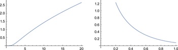
In Figure 3.1, we include plots of
 $\unicode[STIX]{x1D6F7}_{0}$
and
 $\unicode[STIX]{x1D6F7}_{1}$
.
Plot of
 $\unicode[STIX]{x1D6F7}_{0}(r)$
(left) and
 $\unicode[STIX]{x1D6F7}_{1}(r)$
(right).

Proof. Note
 $$\begin{eqnarray}\biggl(\frac{|1/2+\text{i}y|}{-1/2+\text{i}y}\biggr)^{k}=\text{e}^{\text{i}\unicode[STIX]{x1D703}k}=(-1)^{k/2}\text{e}^{-\text{i}k\unicode[STIX]{x1D719}}=(-1)^{k/2}\text{e}^{-\text{i}k\arctan (1/2y)}.\end{eqnarray}$$
In the range
 $y\leqslant k^{2/5}$
, using Corollary 3.5 we derive
 $$\begin{eqnarray}G_{k}(1/2+\text{i}y)=1+\frac{(1/2+\text{i}y)^{k}}{(-1/2+\text{i}y)^{k}}+O(y\exp (-k^{1/5})).\end{eqnarray}$$
Since
 $H_{k}(z)=(|z|/z)^{k}G_{k}(z)$
, we then derive
 $$\begin{eqnarray}H_{k}(1/2+\text{i}y)=2(-1)^{k/2}\cos \biggl(k\arctan \frac{1}{2y}\biggr)+O(y\exp (-k^{1/5})),\end{eqnarray}$$
which gives (3.16).
Now, suppose
 $k^{2/5}<y\leqslant k$
. Then using (3.4) and writing out the definition of the theta function, we have
 $$\begin{eqnarray}H_{k}(1/2+\text{i}y)=(-1)^{k/2}\text{e}^{\text{i}k\arctan (1/2y)}\mathop{\sum }_{n\in \mathbb{Z}}\exp \biggl(-\frac{\unicode[STIX]{x1D70B}}{r}(n^{2}+n)\biggr)\text{e}^{\text{i}nk/y}+O(k^{-2/3}y).\end{eqnarray}$$
Note that
 $n^{2}+n\geqslant 0$
for all
 $n\in \mathbb{Z}$
, and that for
 $n\neq 0,-1$
, then
 $n^{2}+n\geqslant 2$
. Therefore, if
 $r\gg 1$
we get a good approximation by selecting the terms
 $n=0,-1$
, and trivially bounding the rest. This gives
 $$\begin{eqnarray}|H_{k}(1/2+\text{i}y)-(-1)^{k/2}\text{e}^{\text{i}k\arctan (1/2y)}(1+\text{e}^{-\text{i}k/y})|\leqslant \unicode[STIX]{x1D6F7}_{0}(r)+O(k^{-2/3}y).\end{eqnarray}$$
Since
 $y\gg k^{2/5}$
, and
 $\arctan (1/2y)=1/2y+O(y^{-3})$
, we have
 $$\begin{eqnarray}\text{e}^{\text{i}k\arctan (1/2y)}(1+\text{e}^{-\text{i}k/y})=2\cos \biggl(k\arctan \frac{1}{2y}\biggr)+O(k^{-1/5}).\end{eqnarray}$$
This gives (3.18), using
 $k^{-2/3}y\ll k^{-1/6}$
.
In the region
 $k^{1/2}\ll y\leqslant k$
(which implies
 $r\gg 1$
), then we do not get a close approximation by dropping all terms but
 $n=0,-1$
. In this case, we instead use (3.15) in (3.4). We obtain
 $$\begin{eqnarray}\displaystyle H_{k}(1/2+\text{i}y) & = & \displaystyle r^{1/2}\exp \biggl(-\text{i}\unicode[STIX]{x1D703}k-\frac{\text{i}k}{2y}\biggr)\exp \biggl(\frac{\unicode[STIX]{x1D70B}}{4r}\biggr)\mathop{\sum }_{n\in \mathbb{Z}}\nonumber\\ \displaystyle & & \displaystyle \times \,\exp \biggl(-\unicode[STIX]{x1D70B}r\biggl(n-\frac{k}{2\unicode[STIX]{x1D70B}y}\biggr)^{2}\biggr)e(nx)+O(k^{-2/3}y).\nonumber\end{eqnarray}$$
Note that
 $k^{-2/3}y\ll k^{-1/6}r^{1/2}$
, and that
 $\exp (-\text{i}\unicode[STIX]{x1D703}k-\text{i}k/2y)=(-1)^{k/2}(1+O(y^{-3}k))=1+O(k^{-1/2})$
.
Under the additional assumption (3.20), changing variables
 $n\rightarrow n+N$
, and simplifying, we obtain
 $$\begin{eqnarray}\displaystyle H_{k}(1/2+\text{i}y_{N}) & = & \displaystyle (-1)^{N+k/2}r^{1/2}\exp \biggl(\frac{\unicode[STIX]{x1D70B}}{4r}\biggr)\mathop{\sum }_{n\in \mathbb{Z}}(-1)^{n}\nonumber\\ \displaystyle & & \displaystyle \times \,\exp (-\unicode[STIX]{x1D70B}r(n+O(y_{N}^{-1}))^{2})+O(k^{-1/6}r^{1/2}).\end{eqnarray}$$
We now show that in (3.23) we may remove the error term in the exponential without making a new error term. For
 $n=0$
, we have
 $\exp (O(ry_{N}^{-2}))=1+O(k^{-1})$
, which leads to an acceptable error term. Meanwhile, for
 $n\neq 0$
we may assume
 $|n|\ll r^{-1/2}(\log k)^{2}$
, whence
 $r|n|y_{N}^{-1}\ll k^{-1/2}(\log k)^{2}$
. Then we have
 $$\begin{eqnarray}\displaystyle & & \displaystyle \mathop{\sum }_{0<|n|\ll (\log k)^{2}/r^{1/2}}(-1)^{n}\exp (-\unicode[STIX]{x1D70B}r(n+O(y_{N}^{-1}))^{2})\nonumber\\ \displaystyle & & \displaystyle \qquad =\mathop{\sum }_{0<|n|\ll (\log k)^{2}/r^{1/2}}(-1)^{n}\exp (-\unicode[STIX]{x1D70B}rn^{2})(1+O(r|n|y_{N}^{-1}))\nonumber\\ \displaystyle & & \displaystyle \qquad =\mathop{\sum }_{n\neq 0}(-1)^{n}\exp (-\unicode[STIX]{x1D70B}rn^{2})+O(k^{-1/2}).\nonumber\end{eqnarray}$$
That is, we have shown for
 $y_{N}\gg k^{1/2}$
, that
 $$\begin{eqnarray}\displaystyle H_{k}(1/2+\text{i}y_{N}) & = & \displaystyle (-1)^{N+k/2}r^{1/2}\exp \biggl(\frac{\unicode[STIX]{x1D70B}}{4r}\biggr)\nonumber\\ \displaystyle & & \displaystyle \times \,\mathop{\sum }_{n\in \mathbb{Z}}(-1)^{n}\exp (-\unicode[STIX]{x1D70B}rn^{2})+O(r^{1/2}k^{-1/6}).\end{eqnarray}$$
Now the term
 $n=0$
gives a good approximation, so by bounding the tail trivially we obtain (3.21).◻
We shall also find it convenient to record the following “trivial” bound.
Corollary 3.9. Suppose
 $z=1/2+\text{i}y\in {\mathcal{F}}$
with
 $y\leqslant k$
. Then
 $H_{k}(z)\ll (1+y/\sqrt{k})$
.
We shall occasionally find it useful to study derivatives, especially at the corner point
 $\text{e}^{\unicode[STIX]{x1D70B}\text{i}/3}$
. Our first claim is that (3.2) holds uniformly in a sufficiently small neighborhood of
 $z=\text{e}^{\unicode[STIX]{x1D70B}\text{i}/3}$
. Since this point lies on the boundary of
 ${\mathcal{F}}$
, the proofs need to be adjusted slightly. Since our previous analysis was designed to hold for large values of
 $y$
, we found it easiest to revisit the previous proofs. We have the following lemma.
Lemma 3.10. Suppose
 $2/5\leqslant x\leqslant 3/5$
and
 $2^{-1/2}\leqslant y\leqslant 1$
. Then
 $$\begin{eqnarray}G_{k}(z)=1+\frac{z^{k}}{(z-1)^{k}}+\frac{z^{k}}{(z+1)^{k}}+O\biggl(\biggl(\frac{37}{17}\biggr)^{-k/2}\biggr).\end{eqnarray}$$
Proof. The bound (3.7) is valid for
 $z\in \mathbb{H}$
, and shows
 $$\begin{eqnarray}|z|^{k}\mathop{\sum }_{|c|\geqslant 2}\mathop{\sum }_{|d|\geqslant 1}|cz+d|^{-k}\ll \biggl(\frac{|z|^{2}}{4y^{2}}\biggr)^{k/2}\leqslant \biggl(\frac{9/25+y^{2}}{4y^{2}}\biggr)^{k/2}=\biggl(\frac{100}{43}\biggr)^{-k/2},\end{eqnarray}$$
under the additional constraints introduced here. Note
 $100/43>37/17$
. For the terms with
 $|c|=1$
, we use a method similar to the proof of Lemma 3.4, giving
 $$\begin{eqnarray}\displaystyle |z|^{k}\mathop{\sum }_{|d|\geqslant 2}((x+d)^{2}+y^{2})^{-k/2} & \ll & \displaystyle \biggl(\frac{|z|^{2}}{(7/5)^{2}+y^{2}}\biggr)^{k/2}\nonumber\\ \displaystyle & {\leqslant} & \displaystyle \biggl(\frac{(3/5)^{2}+y^{2}}{(7/5)^{2}+y^{2}}\biggr)^{k/2}\leqslant \biggl(\frac{37}{17}\biggr)^{-k/2}.\hspace{34.99677pt}\square\nonumber\end{eqnarray}$$
Using Cauchy’s integral formula, we derive the following.
Corollary 3.11. Suppose
 $2/5\leqslant x\leqslant 3/5$
and
 $2^{-1/2}\leqslant y\leqslant 1$
. Then for
 $j=1,2,\ldots \,$
, we have
 $$\begin{eqnarray}\frac{d^{j}}{dz^{j}}G_{k}(z)=\frac{d^{j}}{dz^{j}}\biggl(1+\frac{z^{k}}{(z-1)^{k}}+\frac{z^{k}}{(z+1)^{k}}\biggr)+O_{j}\biggl(\biggl(\frac{37}{17}\biggr)^{-k/2}\biggr).\end{eqnarray}$$
In our upcoming application, it will be necessary to differentiate
 $H_{k}(z)$
along a curve. Define
 $$\begin{eqnarray}r_{k}(z)=G_{k}(z)-\biggl(1+\frac{z^{k}}{(z-1)^{k}}+\frac{z^{k}}{(z+1)^{k}}\biggr).\end{eqnarray}$$
Lemma 3.12. Suppose that
 $z(t)$
is a smooth curve, defined for
 $t\in (-\unicode[STIX]{x1D700},\unicode[STIX]{x1D700})$
for some small
 $\unicode[STIX]{x1D700}>0$
, whose image is contained within the region
 $2/5\leqslant x\leqslant 3/5$
and
 $2^{-1/2}\leqslant y\leqslant 1$
. Then for
 $j=1,2$
, we have
 $$\begin{eqnarray}\displaystyle \frac{d^{j}}{dt^{j}}H_{k}(z(t))\Bigg|_{t=0} & = & \displaystyle \frac{d^{j}}{dt^{j}}\biggl[\biggl(\frac{|z(t)|}{z(t)}\biggr)^{k}\biggl(1+\frac{z(t)^{k}}{(z(t)-1)^{k}}+\frac{z(t)^{k}}{(z(t)+1)^{k}}\biggr)\biggr]\bigg|_{t=0}\nonumber\\ \displaystyle & & \displaystyle +\,O(2^{-k/2}),\nonumber\end{eqnarray}$$
where the implied constant depends on the curve
 $z(t)$
.
Remark.
In practice, this lemma means that we may safely approximate
 $H_{k}$
by its main term, and differentiate the main term.
Proof. Since
 $H_{k}(z)=(|z|/z)^{k}G_{k}(z)$
, we have
 $$\begin{eqnarray}\displaystyle & & \displaystyle \frac{d}{dt}H_{k}(z(t))-\frac{d}{dt}\biggl[\biggl(\frac{|z(t)|}{z(t)}\biggr)^{k}\biggl(1+\frac{z(t)^{k}}{(z(t)-1)^{k}}+\frac{z(t)^{k}}{(z(t)+1)^{k}}\biggr)\biggr]\nonumber\\ \displaystyle & & \displaystyle \quad =\frac{d}{dt}\biggl(\frac{|z(t)|}{z(t)}\biggr)^{k}r_{k}(z(t)),\nonumber\end{eqnarray}$$
and so it suffices to bound the right-hand side. We have
 $$\begin{eqnarray}\frac{d}{dt}\biggl(\frac{|z(t)|}{z(t)}\biggr)^{k}r_{k}(z(t))=r_{k}(z(t))\frac{d}{dt}\biggl(\frac{|z(t)|}{z(t)}\biggr)^{k}+\biggl(\frac{|z(t)|}{z(t)}\biggr)^{k}r_{k}^{\prime }(z(t))z^{\prime }(t).\end{eqnarray}$$
It is easy to see that
 $$\begin{eqnarray}\frac{d}{dt}\biggl(\frac{|z(t)|}{z(t)}\biggr)^{k}=k\biggl(\frac{|z(t)|}{z(t)}\biggr)^{k-1}\frac{d}{dt}\frac{|z(t)|}{z(t)}\ll k.\end{eqnarray}$$
This proves the desired result for
 $j=1$
. The case
 $j=2$
is similar.◻
Corollary 3.13. Let
 $1/2+\text{i}y=R\text{e}^{\text{i}\unicode[STIX]{x1D703}}$
. Then
 $$\begin{eqnarray}\frac{d}{d\unicode[STIX]{x1D703}}H_{k}(1/2+\text{i}y)|_{\unicode[STIX]{x1D703}=\unicode[STIX]{x1D70B}/3}=\frac{d}{d\unicode[STIX]{x1D703}}2\cos (k\unicode[STIX]{x1D703})|_{\unicode[STIX]{x1D703}=\unicode[STIX]{x1D70B}/3}+O(2^{-k/2}).\end{eqnarray}$$
4 Zeros on the side
To understand the zeros on the line
 $x=1/2$
, we will generally evaluate
 $H_{k}$
at specific sample points.
4.1 Preliminary results
From Corollary 3.8, we shall deduce
Proposition 4.1. Let
 $1/2+\text{i}y_{m}=R\text{e}^{\text{i}\unicode[STIX]{x1D703}_{m}}$
where
 $\unicode[STIX]{x1D703}_{m}=\unicode[STIX]{x1D70B}m/k\in [\unicode[STIX]{x1D70B}/3,\unicode[STIX]{x1D70B}/2)$
. Then
 $\cos (k\unicode[STIX]{x1D703}_{m})=(-1)^{m}$
, and
 $$\begin{eqnarray}\displaystyle & & \displaystyle (-1)^{m}H_{k}(1/2+\text{i}y_{m})\nonumber\\ \displaystyle & & \displaystyle \quad =\left\{\begin{array}{@{}ll@{}}2+\unicode[STIX]{x1D6FE}\unicode[STIX]{x1D6F7}_{0}(r)+O(k^{-1/6}),\quad & y_{m}\leqslant 100k^{1/2},\\ r^{1/2}\exp \biggl({\displaystyle \frac{\unicode[STIX]{x1D70B}}{4r}}\biggr)(1+\unicode[STIX]{x1D6FE}^{\prime }\unicode[STIX]{x1D6F7}_{1}(r))+O(k^{-1/6}r^{1/2}),\quad & {\displaystyle \frac{1}{100}}k^{1/2}\leqslant y_{m}\leqslant k,\end{array}\right.\nonumber\end{eqnarray}$$
where
 $\unicode[STIX]{x1D6FE},\unicode[STIX]{x1D6FE}^{\prime }$
are real numbers of absolute value at most
 $1$
.
From this, one may conclude, in a quantitative way, that the sign of
 $H_{k}(1/2+\text{i}y_{m})$
is the same as
 $(-1)^{m}$
, for all
 $m$
, provided
 $k$
is large enough for the error term to be negligible. A key point is that the set of
 $r$
for which
 $\unicode[STIX]{x1D6F7}_{0}(r)<2$
and
 $\unicode[STIX]{x1D6F7}_{1}(r)<1$
overlap, which is apparent from Figure 3.1.
Proof. For the values of
 $y_{m}$
with
 $y_{m}\leqslant 100k^{1/2}$
, this immediately follows from Corollary 3.8, since
 $\cos (k\unicode[STIX]{x1D703}_{m})=(-1)^{m}$
, so assume
 $y_{m}\gg k^{1/2}$
. Let
 $\unicode[STIX]{x1D719}_{m}=\unicode[STIX]{x1D70B}/2-\unicode[STIX]{x1D703}_{m}=\unicode[STIX]{x1D70B}/2-\unicode[STIX]{x1D70B}m/k$
, so that
 $\tan (\unicode[STIX]{x1D719}_{m})=1/2y_{m}$
. Since
 $y_{m}\gg k^{1/2}$
, this means
 $\unicode[STIX]{x1D719}_{m}\ll k^{-1/2}$
, and so
 $m=k/2-O(k^{1/2})$
(recall that
 $m$
runs over the integers in the interval
 $[k/3,k/2)$
). Say
 $m=k/2-p$
, with
 $p=1,2,\ldots ,P$
with
 $P\ll \sqrt{k}$
. Then by standard Taylor approximations, we have
 $$\begin{eqnarray}\displaystyle y_{m} & = & \displaystyle y_{k/2-p}=\frac{1}{2\tan (\unicode[STIX]{x1D70B}p/k)}=\frac{1}{2(\unicode[STIX]{x1D70B}p/k)(1+O(p^{2}/k^{2}))}\nonumber\\ \displaystyle & = & \displaystyle \frac{k}{2\unicode[STIX]{x1D70B}p}(1+O(k^{-2}p^{2})).\nonumber\end{eqnarray}$$
Since
 $k^{-2}p^{2}\ll k^{-1}$
, this value of
 $y$
satisfies (3.20) with
 $N=p$
, and so the conditions required to apply Corollary 3.8 with
 $y\gg k^{1/2}$
are met. Thus, for
 $y_{m}\gg k^{1/2}$
,
 $H_{k}(1/2+\text{i}y_{m})$
has the same sign as
 $(-1)^{p+k/2}=(-1)^{m}$
, asdesired.◻
We shall need a result analogous to Lemma 2.2.
Lemma 4.2. The function
 $(2\cos (\unicode[STIX]{x1D70B}/3+\unicode[STIX]{x1D70B}/2X))^{X}$
is monotonically increasing for
 $X\geqslant 3$
.
4.2 Proof of Proposition 1.7
We restate Proposition 1.7 for convenience.
Proposition 4.3. Suppose
 $\ell$
is large. Then
 $\unicode[STIX]{x1D6E5}_{k,\ell }$
has at least
 $\lfloor \ell /6\rfloor -1$
zeros on
 $x=1/2$
if
 $\ell \equiv 2,4\hspace{0.6em}({\rm mod}\hspace{0.2em}6)$
, and at least
 $\lfloor \ell /6]-2$
zeros on
 $x=1/2$
if
 $\ell \equiv 0\hspace{0.6em}({\rm mod}\hspace{0.2em}6)$
.
Proof. By direct calculation, we have
 $$\begin{eqnarray}\unicode[STIX]{x1D6E5}_{k,\ell }=E_{k}E_{\ell }-E_{k+\ell }=(E_{k}-1)+(E_{\ell }-1)+(E_{k}-1)(E_{\ell }-1)-(E_{k+\ell }-1).\end{eqnarray}$$
Recalling the definition (3.1), we have
 $$\begin{eqnarray}|z|^{k+\ell }\unicode[STIX]{x1D6E5}_{k,\ell }=|z|^{k}H_{\ell }(z)+|z|^{l}H_{k}(z)+H_{k}(z)H_{\ell }(z)-H_{k+\ell }(z).\end{eqnarray}$$
Suppose that
 $Q_{\ell }$
is the number of integers
 $m$
such that
 $\unicode[STIX]{x1D703}_{m}=\unicode[STIX]{x1D70B}m/\ell \in (\unicode[STIX]{x1D70B}/3,\unicode[STIX]{x1D70B}/2)$
. Let
 $\ell =6q+a$
, where
 $a\in \{0,2,4\}$
, so that
 $m\in (2q+a/3,3q+a/2)$
. Write
 $m=2q+d$
, so that
 $d$
ranges over the following integers:
 $$\begin{eqnarray}\left\{\begin{array}{@{}ll@{}}1\leqslant d\leqslant q-1\quad & \text{if }a=0,\\ 1\leqslant d\leqslant q\quad & \text{if }a=2,\\ 2\leqslant d\leqslant q+1\quad & \text{if }a=4.\end{array}\right.\end{eqnarray}$$
Therefore,
 $$\begin{eqnarray}Q_{\ell }=\left\{\begin{array}{@{}ll@{}}q-1\quad & \text{for }a=0,\\ q\quad & \text{for }a=2,4.\end{array}\right.\end{eqnarray}$$
Our goal is to show that
 $\unicode[STIX]{x1D6E5}_{k,\ell }$
exhibits sign changes along the points
 $1/2+\text{i}y_{m}=R\text{e}^{\text{i}\unicode[STIX]{x1D703}_{m}}$
, which then implies Proposition 4.3.
Suppose
 $k\geqslant \ell$
. Then we rearrange (4.1) as
 $$\begin{eqnarray}|z|^{k+\ell }\unicode[STIX]{x1D6E5}_{k,\ell }(z)=|z|^{k}\biggl(H_{\ell }(z)+\frac{H_{k}(z)}{|z|^{k-\ell }}\biggr)+H_{k}(z)H_{\ell }(z)-H_{k+\ell }(z).\end{eqnarray}$$
If
 $y\gg 1$
, with a large enough implied constant (not depending on
 $k$
or
 $\ell$
), then we claim that
 $|z|^{k+\ell }\unicode[STIX]{x1D6E5}_{k,\ell }(1/2+\text{i}y_{m})$
, with
 $1/2+\text{i}y_{m}=r^{\text{i}\unicode[STIX]{x1D703}_{m}}$
,
 $\unicode[STIX]{x1D703}_{m}=\unicode[STIX]{x1D70B}m/\ell \in (\unicode[STIX]{x1D70B}/3,\unicode[STIX]{x1D70B}/2)$
, has the same sign as
 $(-1)^{m}$
, provided that
 $\ell$
is large enough. For this, we use Corollary 3.9 which then implies
 $$\begin{eqnarray}|z|^{k+\ell }\unicode[STIX]{x1D6E5}_{k,\ell }(z)=|z|^{k}\biggl(\!H_{\ell }(z)+O\biggl(\frac{1+(y/\sqrt{k})}{y^{2}}\biggr)\!\biggr)+O((1+k^{-1/2}y)(1+\ell ^{-1/2}y)),\end{eqnarray}$$
under the additional assumption
 $k>\ell$
, while if
 $k=\ell$
, we simply write
 $$\begin{eqnarray}|z|^{2\ell }\unicode[STIX]{x1D6E5}_{\ell ,\ell }(z)=2|z|^{\ell }H_{\ell }(z)+O((1+\ell ^{-1/2}y)^{2}).\end{eqnarray}$$
In either case, Proposition 4.1 shows that
 $\unicode[STIX]{x1D6E5}_{k,\ell }(1/2+\text{i}y_{m})$
has the same sign as
 $(-1)^{m}$
, for
 $\ell$
large enough, and
 $y$
large enough.
Now, suppose that
 $y\ll 1$
. Then we temporarily forget that
 $y=y_{m}$
, and refer to (3.17), which gives
 $$\begin{eqnarray}|z|^{k+\ell }\unicode[STIX]{x1D6E5}_{k,\ell }(z)=2|z|^{k}P_{k,\ell }(\unicode[STIX]{x1D703})+O(\exp (-\ell ^{1/6})),\end{eqnarray}$$
where
 $z=1/2+\text{i}y=R\text{e}^{\text{i}\unicode[STIX]{x1D703}}$
, and
 $$\begin{eqnarray}P_{k,\ell }(\unicode[STIX]{x1D703})=\cos (\ell \unicode[STIX]{x1D703})+\frac{\cos (k\unicode[STIX]{x1D703})}{|z|^{k-\ell }}+\frac{2\cos (k\unicode[STIX]{x1D703})\cos (\ell \unicode[STIX]{x1D703})-\cos ((k+\ell )\unicode[STIX]{x1D703})}{|z|^{k}}.\end{eqnarray}$$
Now, we express
 $P_{k,\ell }(\unicode[STIX]{x1D703}_{m})$
in terms of the variables
 $q,a,d$
. Writing
 $k-\ell =D$
we derive
 $$\begin{eqnarray}(-1)^{d}P_{k,\ell }(\unicode[STIX]{x1D703}_{m})=1+\frac{\cos (D\unicode[STIX]{x1D703}_{m})}{|z|^{D}}(1+|z|^{-\ell }(-1)^{d}).\end{eqnarray}$$
We also have
 $$\begin{eqnarray}\unicode[STIX]{x1D703}_{m}=\unicode[STIX]{x1D703}_{2q+d}=\frac{\unicode[STIX]{x1D70B}(2q+d)}{6q+a}=\frac{\unicode[STIX]{x1D70B}}{3}+\frac{\unicode[STIX]{x1D70B}}{\ell }\biggl(d-\frac{a}{3}\biggr),\end{eqnarray}$$
and
 $|z|^{-1}=2\cos (\unicode[STIX]{x1D703}_{m})$
. Therefore, with shorthand
 $s=\unicode[STIX]{x1D70B}/\ell (d-a/3)$
, we have
 $\unicode[STIX]{x1D703}_{m}=\unicode[STIX]{x1D70B}/3+s$
, and
 $$\begin{eqnarray}\displaystyle (-1)^{d}P_{k,\ell }(\unicode[STIX]{x1D703}_{m}) & = & \displaystyle 1+\biggl(2\cos \biggl(\frac{\unicode[STIX]{x1D70B}}{3}+s\biggr)\biggr)^{D}\cos \biggl(\frac{D\unicode[STIX]{x1D70B}}{3}+Ds\biggr)\nonumber\\ \displaystyle & & \displaystyle \times \,\biggl[1+(-1)^{d}\biggl(2\cos \biggl(\frac{\unicode[STIX]{x1D70B}}{3}+s\biggr)\biggr)^{\ell }\biggr].\end{eqnarray}$$
We next claim the following.
Proposition 4.4. For all
 $m$
with
 $\unicode[STIX]{x1D703}_{m}\in (\unicode[STIX]{x1D70B}/3,\unicode[STIX]{x1D70B}/2)$
, we have
 $$\begin{eqnarray}(-1)^{m}P_{k,\ell }(\unicode[STIX]{x1D703}_{m})\geqslant 0.17.\end{eqnarray}$$
For
 $\ell$
sufficiently large, using Proposition 4.4 in (4.4) completes the proof of Proposition 4.3.◻
Proof of Proposition 4.4.
First suppose
 $D\equiv 0\hspace{0.6em}({\rm mod}\hspace{0.2em}6)$
. If in addition,
 $s\leqslant \unicode[STIX]{x1D70B}/2D$
then
 $\cos (\unicode[STIX]{x1D70B}D/3+Ds)=\cos (Ds)\geqslant 0$
, so
 $(-1)^{m}P_{k,\ell }(\unicode[STIX]{x1D703}_{m})\geqslant 1$
, which is even stronger than claimed; here we used that the expression in square brackets in (4.6) is
 ${\geqslant}0$
. If instead
 $s>\unicode[STIX]{x1D70B}/2D$
, then
 $$\begin{eqnarray}\biggl(2\cos \biggl(\frac{\unicode[STIX]{x1D70B}}{3}+s\biggr)\biggr)^{D}\leqslant \biggl(2\cos \biggl(\frac{\unicode[STIX]{x1D70B}}{3}+\frac{\unicode[STIX]{x1D70B}}{2D}\biggr)\biggr)^{D}<0.07,\end{eqnarray}$$
where this final inequality arises as follows. By Lemma 4.2, it suffices to evaluate the limit as
 $D\rightarrow \infty$
. For this, we have
 $$\begin{eqnarray}\displaystyle \lim _{D\rightarrow \infty }\biggl(2\cos \biggl(\frac{\unicode[STIX]{x1D70B}}{3}+\frac{\unicode[STIX]{x1D70B}}{2D}\biggr)\biggr)^{D} & = & \displaystyle \lim _{D\rightarrow \infty }\exp \biggl(D\log \biggl(1-\frac{\sqrt{3}\unicode[STIX]{x1D70B}}{2D}+O(D^{-2})\biggr)\biggr)\nonumber\\ \displaystyle & = & \displaystyle \exp \biggl(-\frac{\sqrt{3}\unicode[STIX]{x1D70B}}{2}\biggr)=0.0658\ldots .\nonumber\end{eqnarray}$$
Therefore, we derive
 $$\begin{eqnarray}(-1)^{d}P_{k,\ell }(\unicode[STIX]{x1D703}_{m})\geqslant 1-(0.07)(2)=0.86,\end{eqnarray}$$
consistent with (4.7).
Next suppose
 $D\equiv 2,4\hspace{0.6em}({\rm mod}\hspace{0.2em}6)$
. Using a similar argument in which we separately consider the cases
 $s\leqslant \unicode[STIX]{x1D70B}/12D$
and
 $s>\unicode[STIX]{x1D70B}/12D$
, we obtain at worst that
 $$\begin{eqnarray}(-1)^{d}P_{k,\ell }(\unicode[STIX]{x1D703}_{m})>0.17.\end{eqnarray}$$
◻
4.3 The extra zero
In this section, we prove Theorem 1.10, which is the stage
 $2$
bound. Comparing with Proposition 1.7, we see that when
 $\ell \equiv 0,4\hspace{0.6em}({\rm mod}\hspace{0.2em}6)$
, we need to produce an additional sign change, under appropriate conditions on
 $k,\ell$
. Consulting §4.2, we see that if
 $a=0$
, the sample point nearest to
 $\unicode[STIX]{x1D70B}/3$
is
 $\unicode[STIX]{x1D703}_{2q+1}=\unicode[STIX]{x1D70B}/3+\unicode[STIX]{x1D70B}/\ell$
, and
 $P_{k,\ell }(\unicode[STIX]{x1D703}_{2q+1})<0$
. Meanwhile, for
 $a=4$
, the nearest point is
 $\unicode[STIX]{x1D703}_{2q+2}=\unicode[STIX]{x1D70B}/3+2\unicode[STIX]{x1D70B}/3\ell$
, and
 $P_{k,\ell }(\unicode[STIX]{x1D703}_{2q+2})>0$
.
Let us first examine the easiest cases where
 $\unicode[STIX]{x1D70B}/3$
is an acceptable sample point. If
 $k+\ell \not \equiv 0\hspace{0.6em}({\rm mod}\hspace{0.2em}6)$
, then
 $\unicode[STIX]{x1D6E5}_{k,\ell }(\text{e}^{\unicode[STIX]{x1D70B}\text{i}/3})=0$
, so we need to assume
 $k+\ell \equiv 0\hspace{0.6em}({\rm mod}\hspace{0.2em}6)$
. Then by (4.5), we have
 $$\begin{eqnarray}P_{k,\ell }\biggl(\frac{\unicode[STIX]{x1D70B}}{3}\biggr)=2\cos ^{2}\biggl(\frac{\unicode[STIX]{x1D70B}\ell }{3}\biggr)+2\cos \biggl(\frac{\unicode[STIX]{x1D70B}\ell }{3}\biggr)-1=\left\{\begin{array}{@{}ll@{}}3,\quad & \ell \equiv 0~(\text{mod}~6),\\ -1.5,\quad & \ell \equiv 4~(\text{mod}~6).\end{array}\right.\end{eqnarray}$$
This furnishes the desired additional zero.
Now suppose
 $k+\ell \equiv 4\hspace{0.6em}({\rm mod}\hspace{0.2em}6)$
, which is the case where
 $\unicode[STIX]{x1D6E5}_{k,\ell }$
has a single zero at
 $\text{e}^{\unicode[STIX]{x1D70B}\text{i}/3}$
. Recall that
 $$\begin{eqnarray}|z|^{\ell }\unicode[STIX]{x1D6E5}_{k,\ell }=H_{\ell }(z)+\frac{H_{k}(z)}{|z|^{k-\ell }}+\frac{1}{|z|^{k}}(H_{k}(z)H_{\ell }(z)-H_{k+\ell }(z)),\end{eqnarray}$$
that
 $H_{k}(1/2+\text{i}y)=2\cos (k\unicode[STIX]{x1D703})+O((37/17)^{-k/2})$
, so by Corollary 3.13, that
 $(d/d\unicode[STIX]{x1D703})H_{k}(1/2+\text{i}y)=-2k\sin (k\unicode[STIX]{x1D703})+O(2^{-k/2})$
(and likewise for the second derivative, though this is not necessary for this case). Gathering these facts, we derive
 $$\begin{eqnarray}\frac{d}{d\unicode[STIX]{x1D703}}|z|^{\ell }\unicode[STIX]{x1D6E5}_{k,\ell }(1/2+\text{i}y)|_{\unicode[STIX]{x1D703}=\unicode[STIX]{x1D70B}/3}=\frac{d}{d\unicode[STIX]{x1D703}}P_{k,\ell }(\unicode[STIX]{x1D703})|_{\unicode[STIX]{x1D703}=\unicode[STIX]{x1D70B}/3}+O(k2^{-\ell /2}).\end{eqnarray}$$
By a direct calculation (using Mathematica for simplicity), we derive
 $$\begin{eqnarray}P_{k,\ell }^{\prime }\biggl(\frac{\unicode[STIX]{x1D70B}}{3}\biggr)=\left\{\begin{array}{@{}l@{}}\sqrt{3}(2\ell -k),\quad \ell \equiv 4~(\text{mod}~6),k\equiv 0~(\text{mod}~6),\quad \\ \sqrt{3}(2k-\ell ),\quad \ell \equiv 0~(\text{mod}~6),k\equiv 4~(\text{mod}~6).\quad \end{array}\right.\end{eqnarray}$$
When
 $a=0$
, that is,
 $\ell \equiv 0\hspace{0.6em}({\rm mod}\hspace{0.2em}6)$
, then
 $P_{k,\ell }^{\prime }(\unicode[STIX]{x1D70B}/3)>0$
, since
 $k\geqslant \ell$
, while the nearest sample point to
 $\unicode[STIX]{x1D70B}/3$
had a negative value of
 $P_{k,\ell }$
. Therefore, there exists a positive value of
 $P_{k,\ell }$
near to
 $\unicode[STIX]{x1D70B}/3$
. This exhibits an additional sign change.
For
 $a=4$
, that is,
 $\ell \equiv 4\hspace{0.6em}({\rm mod}\hspace{0.2em}6)$
, then
 $P_{k,\ell }^{\prime }(\unicode[STIX]{x1D70B}/3)<0$
for
 $k>2\ell$
(which, by the way, implies
 $k\geqslant 2\ell +4$
), while the nearest sample point has a positive value of
 $P_{k,\ell }$
, so this will provide an additional sign change here also, provided
 $k2^{-\ell /2}$
is small compared to
 $k-2\ell$
. However, this is always true, since we assume
 $\ell$
is sufficiently large. In all, this provides the additional zero for sufficiently large
 $k$
,
 $\ell$
.
Similarly, for the second derivative, we derive
 $$\begin{eqnarray}P_{k,\ell }^{\prime \prime }\biggl(\frac{\unicode[STIX]{x1D70B}}{3}\biggr)=\left\{\begin{array}{@{}ll@{}}2(2k^{2}-2k(\ell -1)-\ell ^{2}-\ell ),\quad & \ell \equiv 0~(\text{mod}~6),k\equiv 2~(\text{mod}~6),\\ 2(-k^{2}+k(4\ell -1)-\ell ^{2}-\ell ),\quad & \ell \equiv 4~(\text{mod}~6),k\equiv 4~(\text{mod}~6).\end{array}\right.\end{eqnarray}$$
Of course, the first derivative vanishes in this case. Consider the case
 $\ell \equiv 0\hspace{0.6em}({\rm mod}\hspace{0.2em}6)$
. Then the polynomial value satisfies
 $$\begin{eqnarray}2k^{2}+k(-2\ell +1)-\ell ^{2}-\ell =2(k-x_{+})(k-x_{-}),\end{eqnarray}$$
where
 $$\begin{eqnarray}x_{\pm }=\frac{\ell -1\pm \sqrt{3\ell ^{2}+1}}{2}.\end{eqnarray}$$
We see that if
 $k>x_{+}$
, which is precisely the condition
 $k\geqslant \text{sp}_{j}(\ell )$
, then certainly
 $P_{k,\ell }^{\prime \prime }(\unicode[STIX]{x1D70B}/3)\geqslant 2$
. This is much larger than
 $k^{2}2^{-\ell /2}$
unless
 $\ell \ll \log k$
, but in this case, we easily see from the left-hand side of (4.11) that
 $P_{k,\ell }^{\prime \prime }(\unicode[STIX]{x1D70B}/3)\gg k^{2}$
, which is large compared to
 $k^{2}2^{-\ell /2}$
for
 $\ell$
large.
A similar calculation holds for
 $\ell \equiv 4\hspace{0.6em}({\rm mod}\hspace{0.2em}6)$
. We omit the details, since it is nearly identical to the previous case.
4.4 The exceptional extra zero on the arc
Using the same ideas as in §4.3, we may prove the supplementary stage
 $2$
bound, Proposition 1.13, which we restate for convenience.
Proposition 4.5. Suppose that
 $L\leqslant \ell \leqslant k<\text{sp}_{j}(\ell )$
. Then
 $A_{k,\ell }\geqslant N_{k,\ell }^{\prime }+1$
.
There are only three cases where
 $\text{sp}_{j}(\ell )\neq \ell$
, given by the conditions on the right-hand side of (1.4) (if
 $\text{sp}_{j}(\ell )=\ell$
, the conditions of Proposition 1.13 are vacuous).
Proof. The proof here is rather similar to that appearing in §4.3, in that we will estimate the first and second derivatives of
 $M_{k,\ell }(\unicode[STIX]{x1D703})$
at
 $\unicode[STIX]{x1D70B}/3$
. We begin with the claim that
 $$\begin{eqnarray}\frac{d^{a}}{d\unicode[STIX]{x1D703}^{a}}(F_{k}(\unicode[STIX]{x1D703})F_{\ell }(\unicode[STIX]{x1D703})-F_{k+\ell }(\unicode[STIX]{x1D703}))|_{\unicode[STIX]{x1D703}=\unicode[STIX]{x1D70B}/3}=\frac{d^{a}}{d\unicode[STIX]{x1D703}^{a}}M_{k,\ell }(\unicode[STIX]{x1D703})|_{\unicode[STIX]{x1D703}=\unicode[STIX]{x1D70B}/3}+O(k^{a}2^{-\ell /2}),\end{eqnarray}$$
for
 $a=1,2$
. This is similar to, yet even easier than, (4.9), since the use of the chain rule is simpler since
 $G_{k}(z)$
is holomorphic (also one should recall
 $F_{k}(\unicode[STIX]{x1D703})=G_{k}(\text{e}^{\text{i}\unicode[STIX]{x1D703}})$
).
First, suppose that
 $k\equiv 0\hspace{0.6em}({\rm mod}\hspace{0.2em}6)$
and
 $\ell \equiv 4\hspace{0.6em}({\rm mod}\hspace{0.2em}6)$
, whence
 $j\in \{2,8\}$
. In this case, there is a single zero of
 $\unicode[STIX]{x1D6E5}_{k,\ell }$
at
 $\text{e}^{\text{i}\unicode[STIX]{x1D70B}/3}$
, and correspondingly we have
 $M_{k,\ell }(\unicode[STIX]{x1D70B}/3)=0$
. By a tedious but direct calculation, we have
 $$\begin{eqnarray}M_{k,\ell }^{\prime }\biggl(\frac{\unicode[STIX]{x1D70B}}{3}\biggr)=\sqrt{3}(-k+2\ell ),\end{eqnarray}$$
provided
 $j=2$
. If
 $j=8$
, the sign here is reversed. For
 $j=2$
, the nearest sample point to
 $\unicode[STIX]{x1D70B}/3$
had
 $m=2n+1$
, whence
 $M_{k,\ell }(\unicode[STIX]{x1D703}_{2n+1})<0$
, while for
 $j=8$
, the sign here is switched. Thus, if
 $k<2\ell$
, that is,
 $k<\text{sp}_{2}(\ell )$
, then
 $M_{k,\ell }^{\prime }(\unicode[STIX]{x1D70B}/3)>0$
. By similar reasoning to that occuring in §4.3, one can show that
 $(d/d\unicode[STIX]{x1D703})(F_{k}(\unicode[STIX]{x1D703})F_{\ell }(\unicode[STIX]{x1D703})-F_{k+\ell }(\unicode[STIX]{x1D703}))|_{\unicode[STIX]{x1D703}=\unicode[STIX]{x1D70B}/3}>0$
, provided
 $\ell$
is sufficiently large. This provides the desired additional zero. The same argument works for
 $j=8$
with signs reversed.
Next, assume that
 $\ell \equiv 0\hspace{0.6em}({\rm mod}\hspace{0.2em}6)$
and
 $k\equiv 2\hspace{0.6em}({\rm mod}\hspace{0.2em}6)$
, or
 $k\equiv \ell \equiv 4\hspace{0.6em}({\rm mod}\hspace{0.2em}6)$
. In these cases, there is a double zero at
 $\unicode[STIX]{x1D70B}/3$
. By a direct but tedious calculation, we have if
 $\ell \equiv 0\hspace{0.6em}({\rm mod}\hspace{0.2em}6)$
and
 $k\equiv 2\hspace{0.6em}({\rm mod}\hspace{0.2em}6)$
, and
 $j=2$
, then
 $$\begin{eqnarray}M_{k,\ell }^{\prime \prime }\biggl(\frac{\unicode[STIX]{x1D70B}}{3}\biggr)=-2k^{2}+2k(\ell -1)+\ell ^{2}+\ell .\end{eqnarray}$$
If
 $j=8$
, the sign is switched. Up to a factor
 $-2$
, this formula agrees with (4.10), so this provides the desired additional zero for
 $\ell$
large.
In the case
 $k\equiv \ell \equiv 4\hspace{0.6em}({\rm mod}\hspace{0.2em}6)$
, and with
 $j=0$
, we obtain
 $$\begin{eqnarray}M_{k,\ell }^{\prime \prime }\biggl(\frac{\unicode[STIX]{x1D70B}}{3}\biggr)=-k^{2}+k(4\ell -1)-\ell ^{2}-\ell .\end{eqnarray}$$
Again, when
 $j=6$
, the sign here is switched, and again we obtain the same polynomial as in (4.10), up to a factor
 $-2$
. This provides the desired additional zero.◻